Poincaré-Friedrichs Type Constants for Operators Involving
grad, curl, and div: Theory and Numerical Experiments

Abstract.

We give some theoretical as well as computational results on Laplace and Maxwell constants, i.e., on the smallest constants $c_{n}>0$ arising in estimates of the form

$$|u|_{\mathsf{L}^{2}(\Omega)}\leq c_{0}|\operatorname{grad}u|_{\mathsf{L}^{2}(\Omega)},\qquad|E|_{\mathsf{L}^{2}(\Omega)}\leq c_{1}|\operatorname{curl}E|_{\mathsf{L}^{2}(\Omega)},\qquad|H|_{\mathsf{L}^{2}(\Omega)}\leq c_{2}|\operatorname{div}H|_{\mathsf{L}^{2}(\Omega)}.$$

Besides the classical de Rham complex we investigate the complex of elasticity and the complex related to the biharmonic equation and general relativity as well using the general functional analytical concept of Hilbert complexes. We consider mixed boundary conditions and bounded Lipschitz domains of arbitrary topology. Our numerical aspects are presented by examples for the de Rham complex in 2D and 3D which not only confirm our theoretical findings but also indicate some interesting conjectures.

1. Introduction

We present some theoretical results as well as some computations on Laplace and Maxwell constants for bounded Lipschitz domains $\Omega$ with mixed boundary conditions defined on boundary parts $\Gamma_{\!\tau}$ and $\Gamma_{\!\nu}$ of the boundary $\Gamma$. While a lot of our theoretical findings hold for domains $\Omega$ in arbitrary dimensions, we restrict our numerical experiments to the 2D and 3D cases. Moreover, we verify various theoretical results established in the last few years in [37, 38, 39, 41]. There is a recent interest in these eigenvalues, see, e.g., [17, 18, 29] and related contributions [19, 20, 26, 27, 28, 30, 45], but little results for mixed boundary conditions are known in the literature, except for, e.g., [39, 41]. In 3D these constants are the best possible real numbers $c_{0,\Gamma_{\!\tau}}$, $c_{1,\Gamma_{\!\tau}}$, $c_{2,\Gamma_{\!\tau}}>0$ in the estimates

$$\forall\,u \in D(\operatorname{grad}_{\Gamma_{\!\tau}})\cap R(\operatorname{div}_{\Gamma_{\!\nu}}) |u|_{\mathsf{L}^{2}(\Omega)} \leq c_{0,\Gamma_{\!\tau}}|\operatorname{grad}u|_{\mathsf{L}^{2}(\Omega)},$$

$$\forall\,E \in D(\operatorname{curl}_{\Gamma_{\!\tau}})\cap R(\operatorname{curl}_{\Gamma_{\!\nu}}) |E|_{\mathsf{L}^{2}(\Omega)} \leq c_{1,\Gamma_{\!\tau}}|\operatorname{curl}E|_{\mathsf{L}^{2}(\Omega)},$$

$$\forall\,H \in D(\operatorname{div}_{\Gamma_{\!\tau}})\cap R(\operatorname{grad}_{\Gamma_{\!\nu}}) |H|_{\mathsf{L}^{2}(\Omega)} \leq c_{2,\Gamma_{\!\tau}}|\operatorname{div}H|_{\mathsf{L}^{2}(\Omega)},$$

which are often called Poincaré-Friedrichs type constants, cf. Section 2.2 for notations. More precisely, we have

$$\frac{1}{c_{0,\Gamma_{\!\tau}}} =\inf_{0\neq u\in D(\operatorname{grad}_{\Gamma_{\!\tau}})\cap R(\operatorname{div}_{\Gamma_{\!\nu}})}\frac{|\operatorname{grad}u|_{\mathsf{L}^{2}(\Omega)}}{|u|_{\mathsf{L}^{2}(\Omega)}} \text{(Friedrichs/Poincar\'{e} constants)},$$

$$\frac{1}{c_{1,\Gamma_{\!\tau}}} =\inf_{0\neq E\in D(\operatorname{curl}_{\Gamma_{\!\tau}})\cap R(\operatorname{curl}_{\Gamma_{\!\nu}})}\frac{|\operatorname{curl}E|_{\mathsf{L}^{2}(\Omega)}}{|E|_{\mathsf{L}^{2}(\Omega)}} \text{(rotation/Maxwell constants)},$$

$$\frac{1}{c_{2,\Gamma_{\!\tau}}} =\inf_{0\neq H\in D(\operatorname{div}_{\Gamma_{\!\tau}})\cap R(\operatorname{grad}_{\Gamma_{\!\nu}})}\frac{|\operatorname{div}H|_{\mathsf{L}^{2}(\Omega)}}{|H|_{\mathsf{L}^{2}(\Omega)}} \text{(divergence constants)}.$$

We also point out the strong connection to the well known de Rham complex with mixed boundary conditions.

It turns out that in the 3D case, cf. Theorem 2.20, the estimates and equations

$$c_{0,\Gamma}\leq c_{0,\Gamma_{\!\tau}}=c_{2,\Gamma_{\!\nu}},\qquad c_{1,\Gamma_{\!\tau}}=c_{1,\Gamma_{\!\nu}},\qquad c_{0,\Gamma}\leq\min\big{\{}c_{0,\emptyset},\frac{\text{\rm diam}(\Omega)}{\pi}\big{\}}$$

always hold and that in convex domains we even have

$$c_{1,\Gamma}=c_{1,\emptyset}\leq c_{0,\emptyset}\leq\frac{\text{\rm diam}(\Omega)}{\pi}.$$

Here,

$$c_{\mathsf{F}}:=c_{0,\Gamma},\qquad c_{\mathsf{P}}:=c_{0,\emptyset}$$

are the classical Friedrichs and Poincaré constants, respectively, and the constants

$$c_{\mathsf{M,t}}:=c_{1,\Gamma}=c_{1,\emptyset}=:c_{\mathsf{M,n}}$$

are often called tangential (electric) and normal (magnetic) Maxwell constants, respectively. All these constants relate to minimal positive eigenvalues of certain Laplace and Maxwell operators. More precisely,

$$\lambda_{0,\Gamma_{\!\tau}}=\frac{1}{c_{0,\Gamma_{\!\tau}}},\qquad\lambda_{1,\Gamma_{\!\tau}}=\frac{1}{c_{1,\Gamma_{\!\tau}}},\qquad\lambda_{2,\Gamma_{\!\tau}}=\frac{1}{c_{2,\Gamma_{\!\tau}}}$$

are the smallest positive eigenvalues of the first order matrix operators

$$\begin{bmatrix}0&-\operatorname{div}_{\Gamma_{\!\nu}}\\ \operatorname{grad}_{\Gamma_{\!\tau}}&0\end{bmatrix},\qquad\begin{bmatrix}0&\operatorname{curl}_{\Gamma_{\!\nu}}\\ \operatorname{curl}_{\Gamma_{\!\tau}}&0\end{bmatrix},\qquad\begin{bmatrix}0&-\operatorname{grad}_{\Gamma_{\!\nu}}\\ \operatorname{div}_{\Gamma_{\!\tau}}&0\end{bmatrix},$$

respectively, and

(1) $$\lambda_{0,\Gamma_{\!\tau}}^{2},\qquad\lambda_{1,\Gamma_{\!\tau}}^{2},\qquad\lambda_{2,\Gamma_{\!\tau}}^{2}$$

are the smallest positive eigenvalues of the second order operators

(2) $$-\operatorname{div}_{\Gamma_{\!\nu}}\operatorname{grad}_{\Gamma_{\!\tau}},\qquad\operatorname{curl}_{\Gamma_{\!\nu}}\operatorname{curl}_{\Gamma_{\!\tau}},\qquad-\operatorname{grad}_{\Gamma_{\!\nu}}\operatorname{div}_{\Gamma_{\!\tau}},$$

respectively. In 2D, cf. Corollary 2.23, we will see that

$$c_{0,\Gamma}\leq c_{0,\Gamma_{\!\tau}}=c_{1,\Gamma_{\!\nu}}=c_{2,\Gamma_{\!\nu}},\qquad c_{0,\Gamma}\leq\min\big{\{}c_{0,\emptyset},\frac{\text{\rm diam}(\Omega)}{\pi}\big{\}}.$$

Generally, in ND, cf. Theorem 2.25, we have

$$c_{0,\Gamma}\leq c_{0,\Gamma_{\!\tau}}=c_{N-1,\Gamma_{\!\nu}},\qquad c_{q,\Gamma_{\!\tau}}=c_{N-q-1,\Gamma_{\!\nu}},\qquad c_{0,\Gamma}\leq\min\big{\{}c_{0,\emptyset},\frac{\text{\rm diam}(\Omega)}{\pi}\big{\}}$$

and in convex domains

$$c_{q,\Gamma}=c_{N-q-1,\emptyset}\leq c_{0,\emptyset}\leq\frac{\text{\rm diam}(\Omega)}{\pi}.$$

Here, $q=0,\dots,N-1$ and the differential operators $\operatorname{grad}$, $\operatorname{curl}$, and $\operatorname{div}$ are simply replaced by the exterior derivative $\operatorname{d}_{q}$ acting on the rank $q$ of the respective differential form. So far, all findings are related to the ND de Rham complex. We will present more examples and results for the 3D elasticity complex as well as for the 3D biharmonic complex.

In a series of numerical tests we discretize the operators (2) by the finite element method and compute upper bounds for the eigenvalues (1) from generalized eigenvalue systems

$$Ku=\lambda^{2}\,Mu$$

with discretized stiffness and mass matrices $K$ and $M$, respectively. There are also recent interests in guaranteed lower bounds, cf. [22, 21, 56]. In a search for the smallest positive eigenvalue $\lambda^{2}$ we exploit a projection into the range of $K$ for smaller size problems or the nested iteration technique for large size problems. The latter theoretical results are confirmed by computations in 2D for the unit square and the unit L-shape domain as well as in 3D for the unit cube and the unit Fichera corner domain. Note that all three constants $c_{\ell,\Gamma_{\!\tau}}$, $\ell=1,2,3$, grow proportionally to the “radius” of the domain. More precisely, e.g., it holds

$$c_{\ell}(r\cdot\Omega,r\cdot\Gamma_{\!\tau})=r\cdot c_{\ell}(\Omega,\Gamma_{\!\tau})=r\cdot c_{\ell,\Gamma_{\!\tau}},$$

where

$$r\cdot\Omega:=\{r\cdot x\,:\,x\in\Omega\},\qquad r\cdot\Gamma_{\!\tau}:=\{r\cdot x\,:\,x\in\Gamma_{\!\tau}\}$$

for some bounded domain $\Omega\subset\mathbb{R}^{3}$ being star-shaped with respect to the origin. Moreover, we performed some monotonicity tests (with respect to boundary conditions) which are just partially guaranteed by our theoretical findings. To our surprise we found (numerically) much stronger inequalities in (26), see also the related Figure 7, giving rise to some interesting conjectures.

2. Theoretical Results

We shall summarise some basic results from functional analysis and apply those to the classical operators of vector analysis.

2.1. Functional Analysis ToolBox

We start with collecting and citing some results from [42, 40, 43, 39, 41] about the so-called functional analysis toolbox (fa-toolbox).

2.1.1. Preliminaries

Let $\operatorname{A}:D(\operatorname{A})\subset\mathsf{H}_{0}\to\mathsf{H}_{1}$ be a densely defined and closed linear operator with domain of definition $D(\operatorname{A})$ on two Hilbert spaces $\mathsf{H}_{0}$ and $\mathsf{H}_{1}$. Then the adjoint $\operatorname{A}^{*}:D(\operatorname{A}^{*})\subset\mathsf{H}_{1}\to\mathsf{H}_{0}$ is well defined and characterised by

$$\forall\,x\in D(\operatorname{A})\quad\forall\,y\in D(\operatorname{A}^{*})\qquad\langle\operatorname{A}x,y\rangle_{\mathsf{H}_{1}}=\langle x,\operatorname{A}^{*}y\rangle_{\mathsf{H}_{0}}.$$

$\operatorname{A}$ and $\operatorname{A}^{*}$ are both densely defined and closed, but typically unbounded. Often $(\operatorname{A},\operatorname{A}^{*})$ is called a dual pair as $(\operatorname{A}^{*})^{*}=\overline{\operatorname{A}}=\operatorname{A}$. The projection theorem shows

(3) $$\mathsf{H}_{0}=N(\operatorname{A})\oplus_{\mathsf{H}_{0}}\overline{R(\operatorname{A}^{*})},\quad\mathsf{H}_{1}=N(\operatorname{A}^{*})\oplus_{\mathsf{H}_{1}}\overline{R(\operatorname{A})},$$

often called Helmholtz/Hodge/Weyl decompositions, where we introduce the notation $N$ for the kernel (or null space) and $R$ for the range of a linear operator. These orthogonal decompositions reduce the operators $\operatorname{A}$ and $\operatorname{A}^{*}$, leading to the injective operators $\operatorname{\mathcal{A}}:=\operatorname{A}|_{\overline{R(\operatorname{A}^{*})}}$ and $\operatorname{\mathcal{A}}^{*}:=\operatorname{A}^{*}|_{\overline{R(\operatorname{A})}}$, i.e.

$$\operatorname{\mathcal{A}}:D(\operatorname{\mathcal{A}})\subset\overline{R(\operatorname{A}^{*})} \to\overline{R(\operatorname{A})}, D(\operatorname{\mathcal{A}}) =D(\operatorname{\mathcal{A}})\cap\overline{R(\operatorname{A}^{*})},$$

$$\operatorname{\mathcal{A}}^{*}:D(\operatorname{\mathcal{A}}^{*})\subset\overline{R(\operatorname{A})} \to\overline{R(\operatorname{A}^{*})}, D(\operatorname{\mathcal{A}}^{*}) =D(\operatorname{\mathcal{A}}^{*})\cap\overline{R(\operatorname{A})}.$$

Note that

$$\overline{R(\operatorname{A}^{*})}=N(\operatorname{A})^{\bot_{\mathsf{H}_{0}}},\quad\overline{R(\operatorname{A})}=N(\operatorname{A}^{*})^{\bot_{\mathsf{H}_{1}}}$$

and that $\operatorname{\mathcal{A}}$ and $\operatorname{\mathcal{A}}^{*}$ are indeed adjoint to each other, i.e., $(\operatorname{\mathcal{A}},\operatorname{\mathcal{A}}^{*})$ is a dual pair as well. Then the inverse operators

$$\operatorname{\mathcal{A}}^{-1}:R(\operatorname{A})\to D(\operatorname{\mathcal{A}}),\quad(\operatorname{\mathcal{A}}^{*})^{-1}:R(\operatorname{A}^{*})\to D(\operatorname{\mathcal{A}}^{*})$$

are well defined and bijective, but possibly unbounded. Furthermore, by (3) we have the refined Helmholtz type decompositions

(4) $$D(\operatorname{A})=N(\operatorname{A})\oplus_{\mathsf{H}_{0}}D(\operatorname{\mathcal{A}}),\quad D(\operatorname{A}^{*})=N(\operatorname{A}^{*})\oplus_{\mathsf{H}_{1}}D(\operatorname{\mathcal{A}}^{*})$$

and thus we obtain for the ranges

$$R(\operatorname{A})=R(\operatorname{\mathcal{A}}),\quad R(\operatorname{A}^{*})=R(\operatorname{\mathcal{A}}^{*}).$$

2.1.2. Basic Results

The following result is a well known and direct consequence of the closed graph theorem and the closed range theorem.

Lemma 2.1 (fa-toolbox lemma 1).

The following assertions are equivalent:

• $\exists\,c_{\operatorname{A}}\,\,\in(0,\infty)$  $\forall\,x\in D(\operatorname{\mathcal{A}})$     $|x|_{\mathsf{H}_{0}}\leq c_{\operatorname{A}}|\operatorname{A}x|_{\mathsf{H}_{1}}$

• $\exists\,c_{\operatorname{A}^{*}}\in(0,\infty)$  $\forall\,y\in D(\operatorname{\mathcal{A}}^{*})$   $|y|_{\mathsf{H}_{1}}\leq c_{\operatorname{A}^{*}}|\operatorname{A}^{*}y|_{\mathsf{H}_{0}}$

• $R(\operatorname{A})=R(\operatorname{\mathcal{A}})$ is closed in $\mathsf{H}_{1}$.

• $R(\operatorname{A}^{*})=R(\operatorname{\mathcal{A}}^{*})$ is closed in $\mathsf{H}_{0}$.

• $\operatorname{\mathcal{A}}^{-1}:R(\operatorname{A})\to D(\operatorname{\mathcal{A}})$ is bounded by $c_{\operatorname{A}}$.

• $(\operatorname{\mathcal{A}}^{*})^{-1}:R(\operatorname{A}^{*})\to D(\operatorname{\mathcal{A}}^{*})$ is bounded by $c_{\operatorname{A}^{*}}$.

• $\operatorname{\mathcal{A}}:D(\operatorname{\mathcal{A}})\subset R(\operatorname{A}^{*})\to R(\operatorname{A})$ is bijective with continuous inverse.

• $\operatorname{\mathcal{A}}^{*}:D(\operatorname{\mathcal{A}}^{*})\subset R(\operatorname{A})\to R(\operatorname{A}^{*})$ is bijective with continuous inverse.

• $\operatorname{\mathcal{A}}:D(\operatorname{\mathcal{A}})\to R(\operatorname{A})$ is a topological isomorphism.

• $\operatorname{\mathcal{A}}^{*}:D(\operatorname{\mathcal{A}}^{*})\to R(\operatorname{A}^{*})$ is a topological isomorphism.

The latter inequalities will be called Poincaré-Friedrichs type estimates. Note that in (iv) and (iv^∗) we consider $\operatorname{\mathcal{A}}$ and $\operatorname{\mathcal{A}}^{*}$ as unbounded linear operators, whereas in (v) and (v^∗) we consider $\operatorname{\mathcal{A}}$ and $\operatorname{\mathcal{A}}^{*}$ as bounded linear operators.

Lemma 2.2 (fa-toolbox lemma 2).

The following assertions are equivalent:

• $D(\operatorname{\mathcal{A}})\hookrightarrow\mathsf{H}_{0}$ is compact.

• $D(\operatorname{\mathcal{A}}^{*})\hookrightarrow\mathsf{H}_{1}$ is compact.

• $\operatorname{\mathcal{A}}^{-1}:R(\operatorname{A})\to R(\operatorname{A}^{*})$ is compact.

• $(\operatorname{\mathcal{A}}^{*})^{-1}:R(\operatorname{A}^{*})\to R(\operatorname{A})$ is compact.

Moreover: Each of these assumptions imply the assertions of Lemma 2.1 (and of Lemma 2.2).

Remark 2.3 (sufficient assumptions for the fa-toolbox).

• If $R(\operatorname{A})$ is closed, then the assertions of Lemma 2.1 hold.

• If $D(\operatorname{\mathcal{A}})\hookrightarrow\mathsf{H}_{0}$ is compact, then the assertions of Lemma 2.1 and Lemma 2.2 hold. In particular, the Poincaré-Friedrichs type estimates hold, all ranges are closed and the inverse operators are compact.

2.1.3. Constants, Spectra, and Eigenvalues

Let us introduce the “best” constants $c_{\operatorname{A}}$, $c_{\operatorname{A}^{*}}$ by utilising the Rayleigh quotients

(5) $$\frac{1}{c_{\operatorname{A}}}:=\inf_{0\neq x\in D(\operatorname{\mathcal{A}})}\frac{|\operatorname{A}x|_{\mathsf{H}_{1}}}{|x|_{\mathsf{H}_{0}}},\quad\frac{1}{c_{\operatorname{A}^{*}}}:=\inf_{0\neq y\in D(\operatorname{\mathcal{A}}^{*})}\frac{|\operatorname{A}^{*}y|_{\mathsf{H}_{0}}}{|y|_{\mathsf{H}_{1}}}.$$

Then $0<c_{\operatorname{A}},c_{\operatorname{A}^{*}}\leq\infty$ and we refer to $c_{\operatorname{A}}$ and $c_{\operatorname{A}^{*}}$ as Poincaré-Friedrichs type constants. From now on, we assume that we always deal with these best constants.

Lemma 2.4 (constant lemma).

The Poincaré-Friedrichs type constants coincide, i.e., $c_{\operatorname{A}}=c_{\operatorname{A}^{*}}$.

In the case that $R(\operatorname{A})$ is closed, we shall denote

$$\lambda_{\operatorname{A}}:=\frac{1}{c_{\operatorname{A}}}=\frac{1}{c_{\operatorname{A}^{*}}}>0.$$

Let us emphasise that

(6) $$\operatorname{A}^{*}\operatorname{A},\quad\operatorname{A}\operatorname{A}^{*},\quad|\operatorname{A}|,\quad|\operatorname{A}^{*}|,\quad\begin{bmatrix}\operatorname{A}^{*}\operatorname{A}&0\\ 0&\operatorname{A}\operatorname{A}^{*}\end{bmatrix},\quad\begin{bmatrix}\operatorname{A}\operatorname{A}^{*}&0\\ 0&\operatorname{A}^{*}\operatorname{A}\end{bmatrix},\quad\begin{bmatrix}0&\operatorname{A}^{*}\\ \operatorname{A}&0\end{bmatrix},\quad\begin{bmatrix}0&\operatorname{A}\\ \operatorname{A}^{*}&0\end{bmatrix}$$

are self-adjoint, see Appendix 6, and have essentially - except of $0$ and taking square roots - the same spectra contained in $\mathbb{R}$. Moreover, the first four operators are non-negative. The same holds true for the reduced operators $\operatorname{\mathcal{A}}$ and $\operatorname{\mathcal{A}}^{*}$. We will give more details in the next lemma.

Lemma 2.5 (constant and eigenvalue lemma).

Let $D(\operatorname{\mathcal{A}})\hookrightarrow\mathsf{H}_{0}$ be compact. Then the operators in (6) have pure and discrete point spectra with no accumulation point in $\mathbb{R}$. Moreover:

• $\lambda_{\operatorname{A}}$ is the smallest positive eigenvalue of $\begin{bmatrix}0&\operatorname{A}^{*}\\ \operatorname{A}&0\end{bmatrix}$ and of $\begin{bmatrix}0&\operatorname{A}\\ \operatorname{A}^{*}&0\end{bmatrix}$.

• $\lambda_{\operatorname{A}}^{2}$ is the smallest positive eigenvalue of $\operatorname{A}^{*}\operatorname{A}$ and of $\operatorname{A}\operatorname{A}^{*}$.

• $\lambda_{\operatorname{A}}^{2}$ is the smallest positive eigenvalue of $\begin{bmatrix}\operatorname{A}^{*}\operatorname{A}&0\\ 0&\operatorname{A}\operatorname{A}^{*}\end{bmatrix}$ and of $\begin{bmatrix}\operatorname{A}\operatorname{A}^{*}&0\\ 0&\operatorname{A}^{*}\operatorname{A}\end{bmatrix}$.

• $\displaystyle\sigma(\operatorname{A}^{*}\operatorname{A})\setminus\{0\}=\sigma(\operatorname{A}\operatorname{A}^{*})\setminus\{0\}=\sigma\Big{(}\begin{bmatrix}\operatorname{A}^{*}\operatorname{A}&0\\ 0&\operatorname{A}\operatorname{A}^{*}\end{bmatrix}\Big{)}\setminus\{0\}=\sigma\Big{(}\begin{bmatrix}\operatorname{A}\operatorname{A}^{*}&0\\ 0&\operatorname{A}^{*}\operatorname{A}\end{bmatrix}\Big{)}\setminus\{0\}>0$

• $\displaystyle\sigma\Big{(}\begin{bmatrix}0&\operatorname{A}^{*}\\ \operatorname{A}&0\end{bmatrix}\Big{)}\setminus\{0\}=\sigma\Big{(}\begin{bmatrix}0&\operatorname{A}\\ \operatorname{A}^{*}&0\end{bmatrix}\Big{)}\setminus\{0\}=\pm\sqrt{\sigma(\operatorname{A}^{*}\operatorname{A})\setminus\{0\}}$

• $\sigma(\operatorname{A}^{*}\operatorname{A})\setminus\{0\}=\sigma(\operatorname{\mathcal{A}}^{*}\operatorname{\mathcal{A}})$ and corresponding results hold for all other spectra in (iv).

• $\displaystyle\sigma\Big{(}\begin{bmatrix}0&\operatorname{A}^{*}\\ \operatorname{A}&0\end{bmatrix}\Big{)}\setminus\{0\}=\sigma\Big{(}\begin{bmatrix}0&\operatorname{\mathcal{A}}^{*}\\ \operatorname{\mathcal{A}}&0\end{bmatrix}\Big{)}$ and corresponding results hold for all other spectra in (v).

• $\big{|}\operatorname{\mathcal{A}}^{-1}\big{|}_{R(\operatorname{A}),R(\operatorname{A}^{*})}=\big{|}(\operatorname{\mathcal{A}}^{*})^{-1}\big{|}_{R(\operatorname{A}^{*}),R(\operatorname{A})}=c_{\operatorname{A}}$

• $\big{|}\operatorname{\mathcal{A}}^{-1}\big{|}_{R(\operatorname{A}),D(\operatorname{A})}=\big{|}(\operatorname{\mathcal{A}}^{*})^{-1}\big{|}_{R(\operatorname{A}^{*}),D(\operatorname{A}^{*})}=(c_{\operatorname{A}}^{2}+1)^{1/2}$

• $\big{|}(\operatorname{\mathcal{A}}^{*}\operatorname{\mathcal{A}})^{-1}\big{|}_{R(\operatorname{A}^{*}),R(\operatorname{A}^{*})}=\big{|}(\operatorname{\mathcal{A}}\operatorname{\mathcal{A}}^{*})^{-1}\big{|}_{R(\operatorname{A}),R(\operatorname{A})}=c_{\operatorname{A}}^{2}$

• $N(\operatorname{A})=N(\operatorname{A}^{*}\operatorname{A})=N(\operatorname{A}\operatorname{A}^{*}\operatorname{A})=\dots$ and $N(\operatorname{A}^{*})=N(\operatorname{A}\operatorname{A}^{*})=N(\operatorname{A}^{*}\operatorname{A}\operatorname{A}^{*})=\dots$.

• $R(\operatorname{A})=R(\operatorname{A}\operatorname{A}^{*})=R(\operatorname{A}\operatorname{A}^{*}\operatorname{A})=\dots$ and $R(\operatorname{A}^{*})=R(\operatorname{A}^{*}\operatorname{A})=R(\operatorname{A}^{*}\operatorname{A}\operatorname{A}^{*})=\dots$ and the same holds for the operators $\operatorname{\mathcal{A}}$ and $\operatorname{\mathcal{A}}^{*}$.

For a proof see Appendix 6.

Remark 2.6 (variational formulations).

By Lemma 2.5 the infima in (5) are minima, provided that $D(\operatorname{\mathcal{A}})\hookrightarrow\mathsf{H}_{0}$ is compact. In particular, the respective minimisers $x_{\operatorname{A}}$ and $y_{\operatorname{A}}$ are the eigenvectors to the eigenvalue $\lambda_{\operatorname{A}}^{2}$, i.e,

$$\inf_{0\neq x\in D(\operatorname{\mathcal{A}})}\frac{|\operatorname{A}x|_{\mathsf{H}_{1}}}{|x|_{\mathsf{H}_{0}}}=|\operatorname{A}x_{\operatorname{A}}|_{\mathsf{H}_{1}}=\lambda_{\operatorname{A}}=|\operatorname{A}^{*}y_{\operatorname{A}}|_{\mathsf{H}_{0}}=\inf_{0\neq y\in D(\operatorname{\mathcal{A}}^{*})}\frac{|\operatorname{A}^{*}y|_{\mathsf{H}_{0}}}{|y|_{\mathsf{H}_{1}}},$$

where we assume without loss of generality $|x_{\operatorname{A}}|_{\mathsf{H}_{0}}=|y_{\operatorname{A}}|_{\mathsf{H}_{1}}=1$. Moreover,

$$(\operatorname{A}^{*}\operatorname{A}-\lambda_{\operatorname{A}}^{2})x_{\operatorname{A}} =0, x_{\operatorname{A}} \in D(\operatorname{A}^{*}\operatorname{A})\cap R(\operatorname{A}^{*})=D(\operatorname{\mathcal{A}}^{*}\operatorname{\mathcal{A}})\subset D(\operatorname{\mathcal{A}}),$$

$$(\operatorname{A}\operatorname{A}^{*}-\lambda_{\operatorname{A}}^{2})y_{\operatorname{A}} =0, y_{\operatorname{A}} \in D(\operatorname{A}\operatorname{A}^{*})\cap R(\operatorname{A})=D(\operatorname{\mathcal{A}}\operatorname{\mathcal{A}}^{*})\subset D(\operatorname{\mathcal{A}}^{*}),$$

and the eigenvectors satisfy the variational formulations

$$\forall\,\phi \in D(\operatorname{A}) \langle\operatorname{A}x_{\operatorname{A}},\operatorname{A}\phi\rangle_{\mathsf{H}_{1}} =\lambda_{\operatorname{A}}^{2}\langle x_{\operatorname{A}},\phi\rangle_{\mathsf{H}_{0}},$$

$$\forall\,\psi \in D(\operatorname{A}^{*}) \langle\operatorname{A}^{*}y_{\operatorname{A}},\operatorname{A}^{*}\psi\rangle_{\mathsf{H}_{0}} =\lambda_{\operatorname{A}}^{2}\langle y_{\operatorname{A}},\psi\rangle_{\mathsf{H}_{1}}.$$

2.1.4. Complex Structure Results

Now, let

$$\operatorname{A}_{0}\!:\!D(\operatorname{A}_{0})\subset\mathsf{H}_{0}\to\mathsf{H}_{1},\quad\operatorname{A}_{1}\!:\!D(\operatorname{A}_{1})\subset\mathsf{H}_{1}\to\mathsf{H}_{2}$$

be two densely defined and closed linear operators on three Hilbert spaces $\mathsf{H}_{0}$, $\mathsf{H}_{1}$, and $\mathsf{H}_{2}$ with adjoints

$$\operatorname{A}_{0}^{*}\!:\!D(\operatorname{A}_{0}^{*})\subset\mathsf{H}_{1}\to\mathsf{H}_{0},\quad\operatorname{A}_{1}^{*}\!:\!D(\operatorname{A}_{1}^{*})\subset\mathsf{H}_{2}\to\mathsf{H}_{1}$$

as well as reduced operators $\operatorname{\mathcal{A}}_{0}$, $\operatorname{\mathcal{A}}_{0}^{*}$, and $\operatorname{\mathcal{A}}_{1}$, $\operatorname{\mathcal{A}}_{1}^{*}$. Furthermore, we assume the complex property (also called sequence property) of $\operatorname{A}_{0}$ and $\operatorname{A}_{1}$, that is $\operatorname{A}_{1}\operatorname{A}_{0}=0$, i.e.,

(7) $$R(\operatorname{A}_{0})\subset N(\operatorname{A}_{1}),$$

which is equivalent to $\operatorname{A}_{0}^{*}\operatorname{A}_{1}^{*}=0$, i.e., $R(\operatorname{A}_{1}^{*})\subset N(\operatorname{A}_{0}^{*})$. Recall that

$$R(\operatorname{A}_{0})=R(\operatorname{\mathcal{A}}_{0}),\quad R(\operatorname{A}_{0}^{*})=R(\operatorname{\mathcal{A}}_{0}^{*}),\quad R(\operatorname{A}_{1})=R(\operatorname{\mathcal{A}}_{1}),\quad R(\operatorname{A}_{1}^{*})=R(\operatorname{\mathcal{A}}_{1}^{*}).$$

From the Helmholtz type decompositions (3) for $\operatorname{A}=\operatorname{A}_{0}$ and $\operatorname{A}=\operatorname{A}_{1}$ we get in particular

(8) $$\mathsf{H}_{1}=\overline{R(\operatorname{A}_{0})}\oplus_{\mathsf{H}_{1}}N(\operatorname{A}_{0}^{*}),\quad\mathsf{H}_{1}=\overline{R(\operatorname{A}_{1}^{*})}\oplus_{\mathsf{H}_{1}}N(\operatorname{A}_{1}).$$

Introducing the cohomology group

$$N_{0,1}:=N(\operatorname{A}_{1})\cap N(\operatorname{A}_{0}^{*}),$$

we obtain the refined Helmholtz type decompositions

(9) $$\begin{aligned} N(\operatorname{A}_{1})&=\overline{R(\operatorname{A}_{0})}\oplus_{\mathsf{H}_{1}}N_{0,1},&N(\operatorname{A}_{0}^{*})&=\overline{R(\operatorname{A}_{1}^{*})}\oplus_{\mathsf{H}_{1}}N_{0,1},\\ D(\operatorname{A}_{1})&=\overline{R(\operatorname{A}_{0})}\oplus_{\mathsf{H}_{1}}\big{(}D(\operatorname{A}_{1})\cap N(\operatorname{A}_{0}^{*})\big{)},\quad&D(\operatorname{A}_{0}^{*})&=\overline{R(\operatorname{A}_{1}^{*})}\oplus_{\mathsf{H}_{1}}\big{(}D(\operatorname{A}_{0}^{*})\cap N(\operatorname{A}_{1})\big{)},\end{aligned}$$

and therefore

(10) $$\mathsf{H}_{1} =\overline{R(\operatorname{A}_{0})}\oplus_{\mathsf{H}_{1}}N_{0,1}\oplus_{\mathsf{H}_{1}}\overline{R(\operatorname{A}_{1}^{*})}.$$

Let us remark that the first line of (9) can also be written as

$$\overline{R(\operatorname{A}_{0})}=N(\operatorname{A}_{1})\cap N_{0,1}^{\bot_{\mathsf{H}_{1}}},\quad\overline{R(\operatorname{A}_{1}^{*})}=N(\operatorname{A}_{0}^{*})\cap N_{0,1}^{\bot_{\mathsf{H}_{1}}}.$$

Note that (10) can be further refined and specialised, e.g., to

(11) $$\begin{split}D(\operatorname{A}_{1})&=\overline{R(\operatorname{A}_{0})}\oplus_{\mathsf{H}_{1}}N_{0,1}\oplus_{\mathsf{H}_{1}}D(\operatorname{\mathcal{A}}_{1}),\\ D(\operatorname{A}_{0}^{*})&=D(\operatorname{\mathcal{A}}_{0}^{*})\oplus_{\mathsf{H}_{1}}N_{0,1}\oplus_{\mathsf{H}_{1}}\overline{R(\operatorname{A}_{1}^{*})},\\ D(\operatorname{A}_{1})\cap D(\operatorname{A}_{0}^{*})&=D(\operatorname{\mathcal{A}}_{0}^{*})\oplus_{\mathsf{H}_{1}}N_{0,1}\oplus_{\mathsf{H}_{1}}D(\operatorname{\mathcal{A}}_{1}).\end{split}$$

We observe

$$D(\operatorname{\mathcal{A}}_{1}) =D(\operatorname{A}_{1})\cap\overline{R(\operatorname{A}_{1}^{*})}\subset D(\operatorname{A}_{1})\cap N(\operatorname{A}_{0}^{*})\subset D(\operatorname{A}_{1})\cap D(\operatorname{A}_{0}^{*}),$$

$$D(\operatorname{\mathcal{A}}_{0}^{*}) =D(\operatorname{A}_{0}^{*})\cap\overline{R(\operatorname{A}_{0})}\subset D(\operatorname{A}_{0}^{*})\cap N(\operatorname{A}_{1})\subset D(\operatorname{A}_{0}^{*})\cap D(\operatorname{A}_{1}),$$

and using the refined Helmholtz type decompositions (10) and (11) as well as the results of Lemma 2.2 we immediately see:

Lemma 2.7 (fa-toolbox lemma 3).

The following assertions are equivalent:

• $D(\operatorname{\mathcal{A}}_{0})\hookrightarrow\mathsf{H}_{0}$, $D(\operatorname{\mathcal{A}}_{1})\hookrightarrow\mathsf{H}_{1}$, and $N_{0,1}\hookrightarrow\mathsf{H}_{1}$ are compact.

• $D(\operatorname{A}_{1})\cap D(\operatorname{A}_{0}^{*})\hookrightarrow\mathsf{H}_{1}$ is compact.

In this case, the cohomology group $N_{0,1}$ has finite dimension.

We summarise:

Theorem 2.8 (fa-toolbox theorem).

Let the ranges $R(\operatorname{A}_{0})$ and $R(\operatorname{A}_{1})$ be closed. Then all ranges $R(\operatorname{A}_{0})$, $R(\operatorname{A}_{0}^{*})$, and $R(\operatorname{A}_{1})$, $R(\operatorname{A}_{1}^{*})$ are closed, and the corresponding Poincaré-Friedrichs type estimates hold, i.e. there exists positive constants $c_{\operatorname{A}_{0}},c_{\operatorname{A}_{1}}$ such that

$$\forall\,z \in D(\operatorname{\mathcal{A}}_{0})=D(\operatorname{A}_{0})\cap R(\operatorname{A}_{0}^{*}) |z|_{\mathsf{H}_{0}} \leq c_{\operatorname{A}_{0}}|\operatorname{A}_{0}z|_{\mathsf{H}_{1}},$$

$$\forall\,x \in D(\operatorname{\mathcal{A}}_{0}^{*})=D(\operatorname{A}_{0}^{*})\cap R(\operatorname{A}_{0})=D(\operatorname{A}_{0}^{*})\cap N(\operatorname{A}_{1})\cap N_{0,1}^{\bot_{\mathsf{H}_{1}}} |x|_{\mathsf{H}_{1}} \leq c_{\operatorname{A}_{0}}|\operatorname{A}_{0}^{*}x|_{\mathsf{H}_{0}},$$

$$\forall\,x \in D(\operatorname{\mathcal{A}}_{1})=D(\operatorname{A}_{1})\cap R(\operatorname{A}_{1}^{*})=D(\operatorname{A}_{1})\cap N(\operatorname{A}_{0}^{*})\cap N_{0,1}^{\bot_{\mathsf{H}_{1}}} |x|_{\mathsf{H}_{1}} \leq c_{\operatorname{A}_{1}}|\operatorname{A}_{1}x|_{\mathsf{H}_{2}},$$

$$\forall\,y \in D(\operatorname{\mathcal{A}}_{1}^{*})=D(\operatorname{A}_{1}^{*})\cap R(\operatorname{A}_{1}) |y|_{\mathsf{H}_{2}} \leq c_{\operatorname{A}_{1}}|\operatorname{A}_{1}^{*}y|_{\mathsf{H}_{1}},$$

and

$$\forall\,x\in D(\operatorname{A}_{1})\cap D(\operatorname{A}_{0}^{*})\cap N_{0,1}^{\bot_{\mathsf{H}_{1}}}\qquad|x|_{\mathsf{H}_{1}}^{2}\leq c_{\operatorname{A}_{1}}^{2}|\operatorname{A}_{1}x|_{\mathsf{H}_{2}}^{2}+c_{\operatorname{A}_{0}}^{2}|\operatorname{A}_{0}^{*}x|_{\mathsf{H}_{0}}^{2}.$$

Moreover, all refined Helmholtz type decompositions (9)-(11) hold with closed ranges, in particular, e.g.,

$$\mathsf{H}_{1}=R(\operatorname{A}_{0})\oplus_{\mathsf{H}_{1}}N_{0,1}\oplus_{\mathsf{H}_{1}}R(\operatorname{A}_{1}^{*}).$$

Remark 2.9.

Let us define $c_{\operatorname{A}_{0},\operatorname{A}_{1}}>0$ by

$$\frac{1}{c_{\operatorname{A}_{0},\operatorname{A}_{1}}^{2}}:=\inf\frac{|\operatorname{A}_{1}x|_{\mathsf{H}_{2}}^{2}+|\operatorname{A}_{0}^{*}x|_{\mathsf{H}_{0}}^{2}}{|x|_{\mathsf{H}_{0}}^{2}},$$

where the infimum is taken over all $0\neq x\in D(\operatorname{A}_{1})\cap D(\operatorname{A}_{0}^{*})\cap N_{0,1}^{\bot_{\mathsf{H}_{1}}}$. Assuming - as mentioned above - that we always take the best constants, we obtain by Theorem 2.8

$$c_{\operatorname{A}_{0},\operatorname{A}_{1}}=\max\{c_{\operatorname{A}_{0}},c_{\operatorname{A}_{1}}\}.$$

This can be seen as follows: Theorem 2.8 shows $c_{\operatorname{A}_{0},\operatorname{A}_{1}}\leq\max\{c_{\operatorname{A}_{0}},c_{\operatorname{A}_{1}}\}$. On the other hand, for

$$x\in D(\operatorname{\mathcal{A}}_{1})=D(\operatorname{A}_{1})\cap R(\operatorname{A}_{1}^{*})=D(\operatorname{A}_{1})\cap N(\operatorname{A}_{0}^{*})\cap N_{0,1}^{\bot_{\mathsf{H}_{1}}}$$

we have $|x|_{\mathsf{H}_{1}}\leq c_{\operatorname{A}_{0},\operatorname{A}_{1}}|\operatorname{A}_{1}x|_{\mathsf{H}_{2}}$ and hence $c_{\operatorname{A}_{1}}\leq c_{\operatorname{A}_{0},\operatorname{A}_{1}}$. Analogously we get $c_{\operatorname{A}_{0}}\leq c_{\operatorname{A}_{0},\operatorname{A}_{1}}$.

Remark 2.10.

If $D(\operatorname{A}_{1})\cap D(\operatorname{A}_{0}^{*})\hookrightarrow\mathsf{H}_{1}$ is compact, then $D(\operatorname{\mathcal{A}}_{0})\hookrightarrow\mathsf{H}_{0}$, $D(\operatorname{\mathcal{A}}_{1})\hookrightarrow\mathsf{H}_{1}$, and $D(\operatorname{\mathcal{A}}_{0}^{*})\hookrightarrow\mathsf{H}_{1}$, $D(\operatorname{\mathcal{A}}_{1}^{*})\hookrightarrow\mathsf{H}_{2}$ are compact, as well as $\dim N_{0,1}<\infty$. Hence all ranges are closed, see Remark 2.3, and all assertions of Theorem 2.8 hold.

In other words, the primal and dual complex, i.e.,

(12) $$\begin{split}\begin{CD}D(\operatorname{A}_{0})@>{\operatorname{A}_{0}}>{}>D(\operatorname{A}_{1})@>{\operatorname{A}_{1}}>{}>\mathsf{H}_{2},\end{CD}\\ \begin{CD}\mathsf{H}_{0}@<{\operatorname{A}_{0}^{*}}<{}<D(\operatorname{A}_{0}^{*})@<{\operatorname{A}_{1}^{*}}<{}<D(\operatorname{A}_{1}^{*}),\end{CD}\end{split}$$

is a Hilbert complex of closed and densely defined linear operators. The additional assumption that the ranges $R(\operatorname{A}_{0})$ and $R(\operatorname{A}_{1})$ are closed (and so also the ranges $R(\operatorname{A}_{0}^{*})$ and $R(\operatorname{A}_{1}^{*})$) is equivalent to the closedness of the Hilbert complex. Moreover, the complex is exact if and only if $N_{0,1}=\{0\}$. The complex is called compact, if

(13) $$D(\operatorname{A}_{1})\cap D(\operatorname{A}_{0}^{*})\hookrightarrow\mathsf{H}_{1}$$

is compact. Remark 2.10 shows that (13) is the crucial assumption for the complex (12).

Finally, we present some results for the (unbounded linear) operator

$$\operatorname{A}_{0}\operatorname{A}_{0}^{*}+\operatorname{A}_{1}^{*}\operatorname{A}_{1}:D(\operatorname{A}_{0}\operatorname{A}_{0}^{*}+\operatorname{A}_{1}^{*}\operatorname{A}_{1})\subset\mathsf{H}_{1}\to\mathsf{H}_{1}$$

with $D(\operatorname{A}_{0}\operatorname{A}_{0}^{*}+\operatorname{A}_{1}^{*}\operatorname{A}_{1}):=\big{\{}x\in D(\operatorname{A}_{1})\cap D(\operatorname{A}_{0}^{*})\,:\,\operatorname{A}_{1}x\in D(\operatorname{A}_{1}^{*})\,\wedge\,\operatorname{A}_{0}^{*}x\in D(\operatorname{A}_{0})\big{\}}$.

Lemma 2.11 (constant and eigenvalue lemma).

Let $D(\operatorname{A}_{1})\cap D(\operatorname{A}_{0}^{*})\hookrightarrow\mathsf{H}_{1}$ be compact. Then:

• $\operatorname{A}_{0}^{*}\operatorname{A}_{0}$, $\operatorname{A}_{0}\operatorname{A}_{0}^{*}$, $\operatorname{A}_{1}^{*}\operatorname{A}_{1}$, $\operatorname{A}_{1}\operatorname{A}_{1}^{*}$, and $\operatorname{A}_{0}\operatorname{A}_{0}^{*}+\operatorname{A}_{1}^{*}\operatorname{A}_{1}$ are self-adjoint and have pure and discrete point spectra with no accumulation point in $\mathbb{R}$.

• The results of Lemma 2.5 hold for $\operatorname{A}_{0}$ and $\operatorname{A}_{1}$, in particular $\sigma(\operatorname{A}_{0}^{*}\operatorname{A}_{0})\setminus\{0\}=\sigma(\operatorname{A}_{0}\operatorname{A}_{0}^{*})\setminus\{0\}$ and $\sigma(\operatorname{A}_{1}^{*}\operatorname{A}_{1})\setminus\{0\}=\sigma(\operatorname{A}_{1}\operatorname{A}_{1}^{*})\setminus\{0\}$ as well as $N(\operatorname{A}_{0}\operatorname{A}_{0}^{*})=N(\operatorname{A}_{0}^{*})$ and $N(\operatorname{A}_{1}^{*}\operatorname{A}_{1})=N(\operatorname{A}_{1})$.

• $N(\operatorname{A}_{0}\operatorname{A}_{0}^{*}+\operatorname{A}_{1}^{*}\operatorname{A}_{1})=N_{0,1}$ and $R(\operatorname{A}_{0}\operatorname{A}_{0}^{*}+\operatorname{A}_{1}^{*}\operatorname{A}_{1})=N_{0,1}^{\bot_{\mathsf{H}_{1}}}$, in particular the range is closed.

• $\operatorname{A}_{0}\operatorname{A}_{0}^{*}+\operatorname{A}_{1}^{*}\operatorname{A}_{1}:D(\operatorname{A}_{0}\operatorname{A}_{0}^{*}+\operatorname{A}_{1}^{*}\operatorname{A}_{1})\cap N_{0,1}^{\bot_{\mathsf{H}_{1}}}\subset N_{0,1}^{\bot_{\mathsf{H}_{1}}}\to N_{0,1}^{\bot_{\mathsf{H}_{1}}}$ is bijective with compact inverse.

• $\operatorname{A}_{0}\operatorname{A}_{0}^{*}+\operatorname{A}_{1}^{*}\operatorname{A}_{1}:D(\operatorname{A}_{0}\operatorname{A}_{0}^{*}+\operatorname{A}_{1}^{*}\operatorname{A}_{1})\cap N_{0,1}^{\bot_{\mathsf{H}_{1}}}\to N_{0,1}^{\bot_{\mathsf{H}_{1}}}$ is a topological isomorphism.

Moreover, the spectrum of $\operatorname{A}_{0}\operatorname{A}_{0}^{*}+\operatorname{A}_{1}^{*}\operatorname{A}_{1}$ is given by the spectra of $\operatorname{A}_{0}\operatorname{A}_{0}^{*}$ and $\operatorname{A}_{1}^{*}\operatorname{A}_{1}$, i.e.,

• $\sigma(\operatorname{A}_{0}\operatorname{A}_{0}^{*}+\operatorname{A}_{1}^{*}\operatorname{A}_{1})\setminus\{0\}=\big{(}\sigma(\operatorname{A}_{0}^{*}\operatorname{A}_{0})\setminus\{0\}\big{)}\cup\big{(}\sigma(\operatorname{A}_{1}^{*}\operatorname{A}_{1})\setminus\{0\}\big{)}$.

• In particular, the smallest positive eigenvalue of $\operatorname{A}_{0}\operatorname{A}_{0}^{*}+\operatorname{A}_{1}^{*}\operatorname{A}_{1}$ is given by $\min\{\lambda_{\operatorname{A}_{0}}^{2},\lambda_{\operatorname{A}_{1}}^{2}\}$.

For a proof see Appendix 6.

Remark 2.12 (Helmholtz decomposition).

$\operatorname{A}_{0}\operatorname{A}_{0}^{*}+\operatorname{A}_{1}^{*}\operatorname{A}_{1}$ provides the Helmholtz decomposition from Theorem 2.8. To see this, let us denote the orthonormal projector onto the cohomology group $N_{0,1}$ by $\pi_{N_{0,1}}:\mathsf{H}_{1}\to N_{0,1}$. Then, for $x\in\mathsf{H}_{1}$ we have $(1-\pi_{N_{0,1}})x\in N_{0,1}^{\bot_{\mathsf{H}_{1}}}$ and

$$x =\pi_{N_{0,1}}x+(1-\pi_{N_{0,1}})x$$

$$=\pi_{N_{0,1}}x+(\operatorname{A}_{0}\operatorname{A}_{0}^{*}+\operatorname{A}_{1}^{*}\operatorname{A}_{1})(\operatorname{A}_{0}\operatorname{A}_{0}^{*}+\operatorname{A}_{1}^{*}\operatorname{A}_{1})^{-1}(1-\pi_{N_{0,1}})x\in N_{0,1}\oplus_{\mathsf{H}_{1}}R(\operatorname{A}_{0})\oplus_{\mathsf{H}_{1}}R(\operatorname{A}_{1}^{*}).$$

2.2. Laplace and Maxwell Constants in 3D

Now, we specialise to linear acoustics and electromagnetics in 3D, i.e., to the classical operators of the 3D-de Rham complex, cf. (12),

(14) $$\begin{split}\begin{CD}\mathsf{H}_{\Gamma_{\!\tau}}(\operatorname{grad},\Omega)@>{\operatorname{A}_{0}=\operatorname{grad}_{\Gamma_{\!\tau}}}>{}>\mathsf{H}_{\Gamma_{\!\tau}}(\operatorname{curl},\Omega)@>{\operatorname{A}_{1}=\operatorname{curl}_{\Gamma_{\!\tau}}}>{}>\mathsf{H}_{\Gamma_{\!\tau}}(\operatorname{div},\Omega)@>{\operatorname{A}_{2}=\operatorname{div}_{\Gamma_{\!\tau}}}>{}>\mathsf{L}^{2}(\Omega),\end{CD}\\ \begin{CD}\mathsf{L}^{2}(\Omega)@<{\operatorname{A}_{0}^{*}=-\operatorname{div}_{\Gamma_{\!\nu}}}<{}<\mathsf{H}_{\Gamma_{\!\nu}}(\operatorname{div},\Omega)@<{\operatorname{A}_{1}^{*}=\operatorname{curl}_{\Gamma_{\!\nu}}}<{}<\mathsf{H}_{\Gamma_{\!\nu}}(\operatorname{curl},\Omega)@<{\operatorname{A}_{2}^{*}=-\operatorname{grad}_{\Gamma_{\!\nu}}}<{}<\mathsf{H}_{\Gamma_{\!\nu}}(\operatorname{grad},\Omega),\end{CD}\end{split}$$

and apply the fa-toolbox to these operators.

More precisely, let $\Omega\subset\mathbb{R}^{3}$ be a bounded weak Lipschitz domain, see [13, Definition 2.3] for details, with boundary $\Gamma:=\operatorname{\partial}\Omega$, which is divided into two relatively open weak Lipschitz subsets $\Gamma_{\!\tau}$ and $\Gamma_{\!\nu}:=\Gamma\setminus\overline{\Gamma_{\!\tau}}$ (its complement), see [13, Definition 2.5] for details. We shall call $(\Omega,\Gamma_{\!\tau})$ a bounded weak Lipschitz pair. Moreover, if $(\Omega,\Gamma_{\!\tau})$ is a bounded weak Lipschitz pair, so is $(\Omega,\Gamma_{\!\nu})$. Note that strong Lipschitz (graph of Lipschitz functions) implies weak Lipschitz (Lipschitz manifolds) for the boundary as well as for the interface. We introduce the usual Lebesgue and Sobolev spaces by $\mathsf{L}^{2}(\Omega)$ and $\mathsf{H}^{k}(\Omega)$, $k\in\mathbb{N}_{0}$. For $k=1$ we also write

$$\mathsf{H}^{1}(\Omega)=\mathsf{H}(\operatorname{grad},\Omega):=\big{\{}u\in\mathsf{L}^{2}(\Omega):\operatorname{grad}u\in\mathsf{L}^{2}(\Omega)\big{\}}.$$

Homogeneous weak boundary conditions (in the strong sense) are defined by closure of respective test functions, i.e.,

(15) $$\mathsf{H}^{1}_{\Gamma_{\!\tau}}(\Omega)=\mathsf{H}_{\Gamma_{\!\tau}}(\operatorname{grad},\Omega):=\overline{\mathsf{C}^{\infty}_{\Gamma_{\!\tau}}(\Omega)}^{\mathsf{H}(\operatorname{grad},\Omega)},$$

where

$$\mathsf{C}^{\infty}_{\Gamma_{\!\tau}}(\Omega):=\big{\{}u|_{\Omega}:u\in\mathsf{C}^{\infty}(\mathbb{R}^{3}),\,\text{\rm supp}\,u\;\text{\rm compact in }\mathbb{R}^{3},\,\text{\rm dist}(\text{\rm supp}\,u,\Gamma_{\!\tau})>0\big{\}}.$$

Analogously we define (using test vector fields)

$$\mathsf{H}(\operatorname{curl},\Omega),\quad\mathsf{H}_{\Gamma_{\!\tau}}(\operatorname{curl},\Omega),\quad\mathsf{H}(\operatorname{div},\Omega),\quad\mathsf{H}_{\Gamma_{\!\tau}}(\operatorname{div},\Omega).$$

All latter definitions extend to $\Omega\subset\mathbb{R}^{N}$, $N\geq 1$, in an obvious way, see [14, 15] for details. Throughout this paper and until otherwise stated, we shall assume the latter minimal regularity on $\Omega$ and $\Gamma_{\!\tau}$.

Assumption 2.13.

$(\Omega,\Gamma_{\!\tau})$ is a bounded weak Lipschitz pair.

As closures of the respective classical operators of vector analysis defined on test functions/vector fields from $\mathsf{C}^{\infty}_{\Gamma_{\!\tau}}(\Omega)$, we consider the densely defined and closed linear operators

$$\operatorname{A}_{0}:=\operatorname{grad}_{\Gamma_{\!\tau}}:D(\operatorname{grad}_{\Gamma_{\!\tau}})\subset\mathsf{L}^{2}(\Omega) \longrightarrow\mathsf{L}^{2}(\Omega); u \mapsto\operatorname{grad}u,$$

$$\operatorname{A}_{1}:=\operatorname{curl}_{\Gamma_{\!\tau}}:D(\operatorname{curl}_{\Gamma_{\!\tau}})\subset\mathsf{L}^{2}(\Omega) \longrightarrow\mathsf{L}^{2}(\Omega); E \mapsto\operatorname{curl}E,$$

$$\operatorname{A}_{2}:=\operatorname{div}_{\Gamma_{\!\tau}}:D(\operatorname{div}_{\Gamma_{\!\tau}})\subset\mathsf{L}^{2}(\Omega) \longrightarrow\mathsf{L}^{2}(\Omega); H \mapsto\operatorname{div}H,$$

together with their adjoints, see [13, Theorem 4.5, Section 5.2] and [14, 15, Theorem 4.7, Section 5.2],

$$\operatorname{A}^{*}_{0}=\operatorname{grad}_{\Gamma_{\!\tau}}^{*}=-\operatorname{div}_{\Gamma_{\!\nu}}:D(\operatorname{div}_{\Gamma_{\!\nu}})\subset\mathsf{L}^{2}(\Omega) \longrightarrow\mathsf{L}^{2}(\Omega); H \mapsto-\operatorname{div}H,$$

$$\operatorname{A}^{*}_{1}=\operatorname{curl}_{\Gamma_{\!\tau}}^{*}=\operatorname{curl}_{\Gamma_{\!\nu}}:D(\operatorname{curl}_{\Gamma_{\!\nu}})\subset\mathsf{L}^{2}(\Omega) \longrightarrow\mathsf{L}^{2}(\Omega); E \mapsto\operatorname{curl}E,$$

$$\operatorname{A}^{*}_{2}=\operatorname{div}_{\Gamma_{\!\tau}}^{*}=-\operatorname{grad}_{\Gamma_{\!\nu}}:D(\operatorname{grad}_{\Gamma_{\!\nu}})\subset\mathsf{L}^{2}(\Omega) \longrightarrow\mathsf{L}^{2}(\Omega); u \mapsto-\operatorname{grad}u.$$

Note that

$$D(\operatorname{grad}_{\Gamma_{\!\tau}})=\mathsf{H}_{\Gamma_{\!\tau}}(\operatorname{grad},\Omega),\quad D(\operatorname{curl}_{\Gamma_{\!\tau}})=\mathsf{H}_{\Gamma_{\!\tau}}(\operatorname{curl},\Omega),\quad D(\operatorname{div}_{\Gamma_{\!\tau}})=\mathsf{H}_{\Gamma_{\!\tau}}(\operatorname{div},\Omega)$$

and that (14) is indeed a Hilbert complex.

Recently, in [13, 14, 15], Weck’s selection theorem, also known as the Maxwell compactness property, has been shown to hold for such bounded weak Lipschitz domains and mixed boundary conditions.

Theorem 2.14 (Weck’s selection theorem).

The embedding

$$\mathsf{H}_{\Gamma_{\!\tau}}(\operatorname{curl},\Omega)\cap\mathsf{H}_{\Gamma_{\!\nu}}(\operatorname{div},\Omega)\hookrightarrow\mathsf{L}^{2}(\Omega)$$

is compact.

For a proof see [13, 14, 15]. A short historical overview of Weck’s selection theorem is given in the introduction of [13], see also the original paper [58] and [49, 57, 26, 59, 34, 36, 50].

Now, Theorem 2.14 implies that the crucial assumption (13) holds for the operators $\operatorname{A}_{n}$ of the de Rham complex (14), cf. the general complex (12). More precisely, by Theorem 2.14

$$\boldsymbol{\mathrm{(a)}} D(\operatorname{A}_{1})\cap D(\operatorname{A}_{0}^{*}) =\mathsf{H}_{\Gamma_{\!\tau}}(\operatorname{curl},\Omega)\cap\mathsf{H}_{\Gamma_{\!\nu}}(\operatorname{div},\Omega)\hookrightarrow\mathsf{L}^{2}(\Omega)=\mathsf{H}_{1},$$

$$\boldsymbol{\mathrm{(b)}} D(\operatorname{A}_{2})\cap D(\operatorname{A}_{1}^{*}) =\mathsf{H}_{\Gamma_{\!\tau}}(\operatorname{div},\Omega)\cap\mathsf{H}_{\Gamma_{\!\nu}}(\operatorname{curl},\Omega)\hookrightarrow\mathsf{L}^{2}(\Omega)=\mathsf{H}_{2}$$

are compact and, hence, (14) is a compact Hilbert complex. Thus, by Theorem 2.8 and Remark 2.10, all ranges are closed, all corresponding Poincaré-Friedrichs type estimates hold, and all refined Helmholtz type decompositions (9)-(11) hold with closed ranges. In particular, denoting the corresponding constants by

$$\frac{1}{\lambda_{0,\Gamma_{\!\tau}}}:=c_{0,\Gamma_{\!\tau}}:=c_{\operatorname{grad}_{\Gamma_{\!\tau}}}:=c_{\operatorname{A}_{0}} =c_{\operatorname{A}_{0}^{*}}=c_{\operatorname{div}_{\Gamma_{\!\nu}}}=c_{2,\Gamma_{\!\nu}}=\frac{1}{\lambda_{2,\Gamma_{\!\nu}}},$$

(16) $$\frac{1}{\lambda_{1,\Gamma_{\!\tau}}}:=c_{1,\Gamma_{\!\tau}}:=c_{\operatorname{curl}_{\Gamma_{\!\tau}}}:=c_{\operatorname{A}_{1}} =c_{\operatorname{A}_{1}^{*}}=c_{\operatorname{curl}_{\Gamma_{\!\nu}}}=c_{1,\Gamma_{\!\nu}}=\frac{1}{\lambda_{1,\Gamma_{\!\nu}}},$$

$$\frac{1}{\lambda_{2,\Gamma_{\!\tau}}}:=c_{2,\Gamma_{\!\tau}}:=c_{\operatorname{div}_{\Gamma_{\!\tau}}}:=c_{\operatorname{A}_{2}} =c_{\operatorname{A}_{2}^{*}}=c_{\operatorname{grad}_{\Gamma_{\!\nu}}}=c_{0,\Gamma_{\!\nu}}=\frac{1}{\lambda_{0,\Gamma_{\!\nu}}},$$

and introducing the (finite-dimensional) cohomology groups

$$\mathcal{H}_{\mathsf{1}} :=N_{0,1}:=N(\operatorname{A}_{1})\cap N(\operatorname{A}_{0}^{*})=N(\operatorname{curl}_{\Gamma_{\!\tau}})\cap N(\operatorname{div}_{\Gamma_{\!\nu}}),$$

$$\mathcal{H}_{\mathsf{2}} :=N_{1,2}:=N(\operatorname{A}_{2})\cap N(\operatorname{A}_{1}^{*})=N(\operatorname{div}_{\Gamma_{\!\tau}})\cap N(\operatorname{curl}_{\Gamma_{\!\nu}}),$$

the so-called Dirichlet/Neumann fields, we have by Theorem 2.8 and Remark 2.10 the following inequalities:

Theorem 2.15 (Poincaré-Friedrichs type estimates).

It holds

$$\forall\,u \in D(\operatorname{\mathcal{A}}_{0})=D(\operatorname{grad}_{\Gamma_{\!\tau}})\cap R(\operatorname{div}_{\Gamma_{\!\nu}}) |u|_{\mathsf{L}^{2}(\Omega)} \leq c_{0,\Gamma_{\!\tau}}|\operatorname{grad}u|_{\mathsf{L}^{2}(\Omega)},$$

$$\forall\,E \in D(\operatorname{\mathcal{A}}_{0}^{*})=D(\operatorname{div}_{\Gamma_{\!\nu}})\cap R(\operatorname{grad}_{\Gamma_{\!\tau}}) |E|_{\mathsf{L}^{2}(\Omega)} \leq c_{0,\Gamma_{\!\tau}}|\operatorname{div}E|_{\mathsf{L}^{2}(\Omega)},$$

$$\forall\,E \in D(\operatorname{\mathcal{A}}_{1})=D(\operatorname{curl}_{\Gamma_{\!\tau}})\cap R(\operatorname{curl}_{\Gamma_{\!\nu}}) |E|_{\mathsf{L}^{2}(\Omega)} \leq c_{1,\Gamma_{\!\tau}}|\operatorname{curl}E|_{\mathsf{L}^{2}(\Omega)},$$

$$\forall\,H \in D(\operatorname{\mathcal{A}}_{1}^{*})=D(\operatorname{curl}_{\Gamma_{\!\nu}})\cap R(\operatorname{curl}_{\Gamma_{\!\tau}}) |H|_{\mathsf{L}^{2}(\Omega)} \leq c_{1,\Gamma_{\!\tau}}|\operatorname{curl}H|_{\mathsf{L}^{2}(\Omega)},$$

and for all $E\in D(\operatorname{A}_{1})\cap D(\operatorname{A}_{0}^{*})\cap N_{0,1}^{\bot_{\mathsf{H}_{1}}}=D(\operatorname{curl}_{\Gamma_{\!\tau}})\cap D(\operatorname{div}_{\Gamma_{\!\nu}})\cap\mathcal{H}^{\bot_{\mathsf{L}^{2}(\Omega)}}_{\mathsf{1}}$

$$|E|_{\mathsf{L}^{2}(\Omega)}^{2}\leq c_{1,\Gamma_{\!\tau}}^{2}|\operatorname{curl}E|_{\mathsf{L}^{2}(\Omega)}^{2}+c_{0,\Gamma_{\!\tau}}^{2}|\operatorname{div}E|_{\mathsf{L}^{2}(\Omega)}^{2},$$

where

$$R(\operatorname{grad}_{\Gamma_{\!\tau}}) =N(\operatorname{curl}_{\Gamma_{\!\tau}})\cap\mathcal{H}^{\bot_{\mathsf{L}^{2}(\Omega)}}_{\mathsf{1}}, R(\operatorname{curl}_{\Gamma_{\!\nu}}) =N(\operatorname{div}_{\Gamma_{\!\nu}})\cap\mathcal{H}^{\bot_{\mathsf{L}^{2}(\Omega)}}_{\mathsf{1}},$$

$$R(\operatorname{grad}_{\Gamma_{\!\nu}}) =N(\operatorname{curl}_{\Gamma_{\!\nu}})\cap\mathcal{H}^{\bot_{\mathsf{L}^{2}(\Omega)}}_{\mathsf{2}}, R(\operatorname{curl}_{\Gamma_{\!\tau}}) =N(\operatorname{div}_{\Gamma_{\!\tau}})\cap\mathcal{H}^{\bot_{\mathsf{L}^{2}(\Omega)}}_{\mathsf{2}}.$$

Let $c_{0,1,\Gamma_{\!\tau}}:=c_{\operatorname{grad}_{\Gamma_{\!\tau}},\operatorname{curl}_{\Gamma_{\!\tau}}}>0$ be defined by

$$\frac{1}{c_{0,1,\Gamma_{\!\tau}}^{2}}:=\inf\frac{|\operatorname{curl}E|_{\mathsf{L}^{2}(\Omega)}^{2}+|\operatorname{div}E|_{\mathsf{L}^{2}(\Omega)}^{2}}{|E|_{\mathsf{L}^{2}(\Omega)}^{2}},$$

where the infimum taken over all $0\neq E\in D(\operatorname{curl}_{\Gamma_{\!\tau}})\cap D(\operatorname{div}_{\Gamma_{\!\nu}})\cap\mathcal{H}^{\bot_{\mathsf{L}^{2}(\Omega)}}_{\mathsf{1}}$.

Remark 2.16.

By Remark 2.9 it holds $c_{0,1,\Gamma_{\!\tau}}=\max\{c_{0,\Gamma_{\!\tau}},c_{1,\Gamma_{\!\tau}}\}$.

Note that by the symmetry of the de Rham complex the corresponding two estimates for $\operatorname{\mathcal{A}}_{2}$ and $\operatorname{\mathcal{A}}_{2}^{*}$, i.e.,

$$\forall\,H \in D(\operatorname{\mathcal{A}}_{2})=D(\operatorname{div}_{\Gamma_{\!\tau}})\cap R(\operatorname{grad}_{\Gamma_{\!\nu}}) |H|_{\mathsf{L}^{2}(\Omega)} \leq c_{2,\Gamma_{\!\tau}}|\operatorname{div}H|_{\mathsf{L}^{2}(\Omega)},$$

$$\forall\,u \in D(\operatorname{\mathcal{A}}_{2}^{*})=D(\operatorname{grad}_{\Gamma_{\!\nu}})\cap R(\operatorname{div}_{\Gamma_{\!\tau}}) |u|_{\mathsf{L}^{2}(\Omega)} \leq c_{2,\Gamma_{\!\tau}}|\operatorname{grad}u|_{\mathsf{L}^{2}(\Omega)},$$

are redundant, as these are already included in the two estimates for $\operatorname{\mathcal{A}}_{0}$ and $\operatorname{\mathcal{A}}_{0}^{*}$ just by interchanging the boundary conditions on $\Gamma_{\!\tau}$ and $\Gamma_{\!\nu}$. In other words, $c_{2,\Gamma_{\!\tau}}=c_{0,\Gamma_{\!\nu}}$. Furthermore,

$$N(\operatorname{grad}_{\Gamma_{\!\tau}}) \;=\begin{cases}\{0\}&\text{if }\Gamma_{\!\tau}\neq\emptyset,\\ \mathbb{R}&\text{if }\Gamma_{\!\tau}=\emptyset,\end{cases}$$

$$R(\operatorname{div}_{\Gamma_{\!\nu}})=N(\operatorname{grad}_{\Gamma_{\!\tau}})^{\bot_{\mathsf{L}^{2}(\Omega)}}=\mathsf{L}^{2}_{\Gamma_{\!\nu}}(\Omega) :=\begin{cases}\mathsf{L}^{2}(\Omega)&\text{if }\Gamma_{\!\nu}\neq\Gamma,\\ \mathsf{L}^{2}(\Omega)\cap\mathbb{R}^{\bot_{\mathsf{L}^{2}(\Omega)}}&\text{if }\Gamma_{\!\nu}=\Gamma,\end{cases}$$

where

$$\mathsf{L}^{2}(\Omega)\cap\mathbb{R}^{\bot_{\mathsf{L}^{2}(\Omega)}}=\big{\{}u\in\mathsf{L}^{2}(\Omega):\langle u,1\rangle_{\mathsf{L}^{2}(\Omega)}=0\big{\}}=\big{\{}u\in\mathsf{L}^{2}(\Omega):\int_{\Omega}u=0\big{\}}.$$

Combinations of the latter operators give the well known operators from acoustics, Maxwell equations, Laplace equations, and the double rotation equations, i.e.,

$$\operatorname{M}_{0} :=\begin{bmatrix}0&\operatorname{A}_{0}^{*}\\ \operatorname{A}_{0}&0\end{bmatrix}=\begin{bmatrix}0&\operatorname{grad}_{\Gamma_{\!\tau}}^{*}\\ \operatorname{grad}_{\Gamma_{\!\tau}}&0\end{bmatrix}=\begin{bmatrix}0&-\operatorname{div}_{\Gamma_{\!\nu}}\\ \operatorname{grad}_{\Gamma_{\!\tau}}&0\end{bmatrix},$$

$$\operatorname{M}_{1} :=\begin{bmatrix}0&\operatorname{A}_{1}^{*}\\ \operatorname{A}_{1}&0\end{bmatrix}=\begin{bmatrix}0&\operatorname{curl}_{\Gamma_{\!\tau}}^{*}\\ \operatorname{curl}_{\Gamma_{\!\tau}}&0\end{bmatrix}=\begin{bmatrix}0&\operatorname{curl}_{\Gamma_{\!\nu}}\\ \operatorname{curl}_{\Gamma_{\!\tau}}&0\end{bmatrix},$$

$$\operatorname{M}_{2} :=\begin{bmatrix}0&\operatorname{A}_{2}^{*}\\ \operatorname{A}_{2}&0\end{bmatrix}=\begin{bmatrix}0&\operatorname{div}_{\Gamma_{\!\tau}}^{*}\\ \operatorname{div}_{\Gamma_{\!\tau}}&0\end{bmatrix}=\begin{bmatrix}0&-\operatorname{grad}_{\Gamma_{\!\nu}}\\ \operatorname{div}_{\Gamma_{\!\tau}}&0\end{bmatrix},$$

and

$$\operatorname{A}_{0}^{*}\operatorname{A}_{0} =\operatorname{grad}_{\Gamma_{\!\tau}}^{*}\operatorname{grad}_{\Gamma_{\!\tau}}=-\operatorname{div}_{\Gamma_{\!\nu}}\operatorname{grad}_{\Gamma_{\!\tau}}=:-\Delta_{\Gamma_{\!\tau}}, \operatorname{A}_{0}\operatorname{A}_{0}^{*} =\operatorname{grad}_{\Gamma_{\!\tau}}\operatorname{grad}_{\Gamma_{\!\tau}}^{*}=-\operatorname{grad}_{\Gamma_{\!\tau}}\operatorname{div}_{\Gamma_{\!\nu}}=-\Diamond_{\Gamma_{\!\nu}},$$

$$\operatorname{A}_{1}^{*}\operatorname{A}_{1} =\operatorname{curl}_{\Gamma_{\!\tau}}^{*}\operatorname{curl}_{\Gamma_{\!\tau}}=\operatorname{curl}_{\Gamma_{\!\nu}}\operatorname{curl}_{\Gamma_{\!\tau}}=:\Box_{\Gamma_{\!\tau}}, \operatorname{A}_{1}\operatorname{A}_{1}^{*} =\operatorname{curl}_{\Gamma_{\!\tau}}\operatorname{curl}_{\Gamma_{\!\tau}}^{*}=\operatorname{curl}_{\Gamma_{\!\tau}}\operatorname{curl}_{\Gamma_{\!\nu}}=\square_{\Gamma_{\!\nu}},$$

$$\operatorname{A}_{2}^{*}\operatorname{A}_{2} =\operatorname{div}_{\Gamma_{\!\tau}}^{*}\operatorname{div}_{\Gamma_{\!\tau}}=-\operatorname{grad}_{\Gamma_{\!\nu}}\operatorname{div}_{\Gamma_{\!\tau}}=:-\Diamond_{\Gamma_{\!\tau}}, \operatorname{A}_{2}\operatorname{A}_{2}^{*} =\operatorname{div}_{\Gamma_{\!\tau}}\operatorname{div}_{\Gamma_{\!\tau}}^{*}=-\operatorname{div}_{\Gamma_{\!\tau}}\operatorname{grad}_{\Gamma_{\!\nu}}=-\Delta_{\Gamma_{\!\nu}}.$$

Again, $\operatorname{M}_{2}$ and the operators involving $\operatorname{A}_{2}$, $\operatorname{A}_{2}^{*}$ are redundant by interchanging the boundary conditions in $\operatorname{M}_{0}$ and $\operatorname{A}_{0}$, $\operatorname{A}_{0}^{*}$. Hence, we may focus on $c_{0,\Gamma_{\!\tau}}$ and $c_{1,\Gamma_{\!\tau}}$. Section 2.1.3 shows the following:

Theorem 2.17 (Poincaré-Friedrichs type constants).

The Poincaré-Friedrichs type constants can be computed by the four Rayleigh quotations

$$\frac{1}{c_{0,\Gamma_{\!\tau}}}=\lambda_{0,\Gamma_{\!\tau}} =\inf_{0\neq u\in D(\operatorname{grad}_{\Gamma_{\!\tau}})\cap\mathsf{L}^{2}_{\Gamma_{\!\nu}}(\Omega)}\frac{|\operatorname{grad}u|_{\mathsf{L}^{2}(\Omega)}}{|u|_{\mathsf{L}^{2}(\Omega)}}=\inf_{0\neq E\in D(\operatorname{div}_{\Gamma_{\!\nu}})\cap R(\operatorname{grad}_{\Gamma_{\!\tau}})}\frac{|\operatorname{div}E|_{\mathsf{L}^{2}(\Omega)}}{|E|_{\mathsf{L}^{2}(\Omega)}},$$

$$\frac{1}{c_{1,\Gamma_{\!\tau}}}=\lambda_{1,\Gamma_{\!\tau}} =\inf_{0\neq E\in D(\operatorname{curl}_{\Gamma_{\!\tau}})\cap R(\operatorname{curl}_{\Gamma_{\!\nu}})}\frac{|\operatorname{curl}E|_{\mathsf{L}^{2}(\Omega)}}{|E|_{\mathsf{L}^{2}(\Omega)}}=\inf_{0\neq H\in D(\operatorname{curl}_{\Gamma_{\!\nu}})\cap R(\operatorname{curl}_{\Gamma_{\!\tau}})}\frac{|\operatorname{curl}H|_{\mathsf{L}^{2}(\Omega)}}{|H|_{\mathsf{L}^{2}(\Omega)}}.$$

Moreover, $\lambda_{0,\Gamma_{\!\tau}}$ is the smallest positive eigenvalue of

$$\begin{bmatrix}0&\operatorname{A}_{0}^{*}\\ \operatorname{A}_{0}&0\end{bmatrix}=\begin{bmatrix}0&-\operatorname{div}_{\Gamma_{\!\nu}}\\ \operatorname{grad}_{\Gamma_{\!\tau}}&0\end{bmatrix}$$

and $\lambda_{0,\Gamma_{\!\tau}}^{2}$ is the smallest (positive) eigenvalue of

$$\operatorname{A}_{0}^{*}\operatorname{A}_{0}=-\operatorname{div}_{\Gamma_{\!\nu}}\operatorname{grad}_{\Gamma_{\!\tau}}=-\Delta_{\Gamma_{\!\tau}}\quad\text{and}\quad\operatorname{A}_{0}\operatorname{A}_{0}^{*}=-\operatorname{grad}_{\Gamma_{\!\tau}}\operatorname{div}_{\Gamma_{\!\nu}}=-\Diamond_{\Gamma_{\!\nu}}.$$

$\lambda_{1,\Gamma_{\!\tau}}$ is the smallest positive eigenvalue of

$$\begin{bmatrix}0&\operatorname{A}_{1}^{*}\\ \operatorname{A}_{1}&0\end{bmatrix}=\begin{bmatrix}0&\operatorname{curl}_{\Gamma_{\!\nu}}\\ \operatorname{curl}_{\Gamma_{\!\tau}}&0\end{bmatrix}$$

and $\lambda_{1,\Gamma_{\!\tau}}^{2}$ is the smallest (positive) eigenvalue of

$$\operatorname{A}_{1}^{*}\operatorname{A}_{1}=\operatorname{curl}_{\Gamma_{\!\nu}}\operatorname{curl}_{\Gamma_{\!\tau}}=\square_{\Gamma_{\!\tau}}\quad\text{and}\quad\operatorname{A}_{1}\operatorname{A}_{1}^{*}=\operatorname{curl}_{\Gamma_{\!\tau}}\operatorname{curl}_{\Gamma_{\!\nu}}=\square_{\Gamma_{\!\nu}}.$$

Remark 2.18 (variational formulations).

All infima in Theorem 2.17 are minima and the respective minimisers $u_{0,\Gamma_{\!\tau}}$, $E_{0,\Gamma_{\!\nu}}$, and $E_{1,\Gamma_{\!\tau}}$, $H_{1,\Gamma_{\!\nu}}$ are the eigenfunctions to the eigenvalues $\lambda_{0,\Gamma_{\!\tau}}^{2}$ and $\lambda_{1,\Gamma_{\!\tau}}^{2}$, i.e,

$$\lambda_{0,\Gamma_{\!\tau}}=\frac{|\operatorname{grad}u_{0,\Gamma_{\!\tau}}|_{\mathsf{L}^{2}(\Omega)}}{|u_{0,\Gamma_{\!\tau}}|_{\mathsf{L}^{2}(\Omega)}}=\frac{|\operatorname{div}E_{0,\Gamma_{\!\nu}}|_{\mathsf{L}^{2}(\Omega)}}{|E_{0,\Gamma_{\!\nu}}|_{\mathsf{L}^{2}(\Omega)}},\qquad\lambda_{1,\Gamma_{\!\tau}}=\frac{|\operatorname{curl}E_{1,\Gamma_{\!\tau}}|_{\mathsf{L}^{2}(\Omega)}}{|E_{1,\Gamma_{\!\tau}}|_{\mathsf{L}^{2}(\Omega)}}=\frac{|\operatorname{curl}H_{1,\Gamma_{\!\nu}}|_{\mathsf{L}^{2}(\Omega)}}{|H_{1,\Gamma_{\!\nu}}|_{\mathsf{L}^{2}(\Omega)}},$$

$$(-\Delta_{\Gamma_{\!\tau}}-\lambda_{0,\Gamma_{\!\tau}}^{2})u_{0,\Gamma_{\!\tau}} =0, u_{0,\Gamma_{\!\tau}} \in D(\Delta_{\Gamma_{\!\tau}})\cap\mathsf{L}^{2}_{\Gamma_{\!\nu}}(\Omega)\subset D(\operatorname{grad}_{\Gamma_{\!\tau}})\cap\mathsf{L}^{2}_{\Gamma_{\!\nu}}(\Omega),$$

$$(-\Diamond_{\Gamma_{\!\nu}}-\lambda_{0,\Gamma_{\!\tau}}^{2})E_{0,\Gamma_{\!\nu}} =0, E_{0,\Gamma_{\!\nu}} \in D(\Diamond_{\Gamma_{\!\nu}})\cap R(\operatorname{grad}_{\Gamma_{\!\tau}})\subset D(\operatorname{div}_{\Gamma_{\!\nu}})\cap R(\operatorname{grad}_{\Gamma_{\!\tau}}),$$

$$(\square_{\Gamma_{\!\tau}}-\lambda_{1,\Gamma_{\!\tau}}^{2})E_{1,\Gamma_{\!\tau}} =0, E_{1,\Gamma_{\!\tau}} \in D(\square_{\Gamma_{\!\tau}})\cap R(\operatorname{curl}_{\Gamma_{\!\nu}})\subset D(\operatorname{curl}_{\Gamma_{\!\tau}})\cap R(\operatorname{curl}_{\Gamma_{\!\nu}}),$$

$$(\square_{\Gamma_{\!\nu}}-\lambda_{1,\Gamma_{\!\tau}}^{2})H_{1,\Gamma_{\!\nu}} =0, H_{1,\Gamma_{\!\nu}} \in D(\square_{\Gamma_{\!\nu}})\cap R(\operatorname{curl}_{\Gamma_{\!\tau}})\subset D(\operatorname{curl}_{\Gamma_{\!\nu}})\cap R(\operatorname{curl}_{\Gamma_{\!\tau}}).$$

Moreover, the eigenvectors satisfy the variational formulations

$$\forall\,\psi \in D(\operatorname{grad}_{\Gamma_{\!\tau}}) \langle\operatorname{grad}u_{0,\Gamma_{\!\tau}},\operatorname{grad}\psi\rangle_{\mathsf{L}^{2}(\Omega)} =\lambda_{0,\Gamma_{\!\tau}}^{2}\langle u_{0,\Gamma_{\!\tau}},\psi\rangle_{\mathsf{L}^{2}(\Omega)},$$

$$\forall\,\Psi \in D(\operatorname{div}_{\Gamma_{\!\nu}}) \langle\operatorname{div}E_{0,\Gamma_{\!\nu}},\operatorname{div}\Psi\rangle_{\mathsf{L}^{2}(\Omega)} =\lambda_{0,\Gamma_{\!\tau}}^{2}\langle E_{0,\Gamma_{\!\nu}},\Psi\rangle_{\mathsf{L}^{2}(\Omega)},$$

$$\forall\,\Phi \in D(\operatorname{curl}_{\Gamma_{\!\tau}}) \langle\operatorname{curl}E_{1,\Gamma_{\!\tau}},\operatorname{curl}\Phi\rangle_{\mathsf{L}^{2}(\Omega)} =\lambda_{1,\Gamma_{\!\tau}}^{2}\langle E_{1,\Gamma_{\!\tau}},\Phi\rangle_{\mathsf{L}^{2}(\Omega)},$$

$$\forall\,\Theta \in D(\operatorname{curl}_{\Gamma_{\!\nu}}) \langle\operatorname{curl}H_{1,\Gamma_{\!\nu}},\operatorname{curl}\Theta\rangle_{\mathsf{L}^{2}(\Omega)} =\lambda_{1,\Gamma_{\!\tau}}^{2}\langle H_{1,\Gamma_{\!\nu}},\Theta\rangle_{\mathsf{L}^{2}(\Omega)}.$$

Remark 2.19.

We emphasise that Lemma 2.11 provides results for the vector Laplacian

$$\operatorname{A}_{0}\operatorname{A}_{0}^{*}+\operatorname{A}_{1}^{*}\operatorname{A}_{1}=-\Diamond_{\Gamma_{\!\nu}}+\square_{\Gamma_{\!\tau}}=-\operatorname{grad}_{\Gamma_{\!\tau}}\operatorname{div}_{\Gamma_{\!\nu}}+\operatorname{curl}_{\Gamma_{\!\nu}}\operatorname{curl}_{\Gamma_{\!\tau}},$$

which has been recently discussed in, e.g., [25].

2.2.1. Known Results for the Constants in 3D

Let us summarise and cite some recent results from [37, 38, 39, 41] about the Poincaré-Friedrichs type constants, i.e., about the Poincaré-Friedrichs constants $\lambda_{0,\Gamma_{\!\tau}}$ and the Maxwell constants $\lambda_{1,\Gamma_{\!\tau}}$.

Theorem 2.20 (Poincaré-Friedrichs/Maxwell constants in 3D).

For $c_{\ell,\Gamma_{\!\tau}}=1/\lambda_{\ell,\Gamma_{\!\tau}}$ the following holds:

• The Poincaré-Friedrichs constants depend monotonically on the boundary conditions, i.e.,

  $$\emptyset\neq\widetilde{\Gamma}_{\tau}\subset\Gamma_{\!\tau}\quad\Rightarrow\quad c_{0,\Gamma_{\!\tau}}\leq c_{0,\widetilde{\Gamma}_{\tau}}.$$

• The Friedrichs constant is always smaller than the Poincaré constant, i.e.,

  $$c_{0,\Gamma}\leq c_{0,\emptyset},$$

  where $c_{0,\Gamma}$ is the classical Friedrichs constant and $c_{0,\emptyset}$ is the classical Poincaré constant. Moreover, $\lambda_{0,\Gamma}$ is usually called the first Dirichlet-Laplace eigenvalue and $\lambda_{0,\emptyset}$ is usually called the second Neumann-Laplace eigenvalue.

• $c_{0,\Gamma}\leq\text{\rm diam}(\Omega)/\pi$

• $c_{0,\Gamma_{\!\tau}}=c_{2,\Gamma_{\!\nu}}$

• $c_{1,\Gamma_{\!\tau}}=c_{1,\Gamma_{\!\nu}}$

• $c_{0,\Gamma}\leq c_{0,\Gamma_{\!\tau}}\leq c_{0,1,\Gamma_{\!\tau}}=\max\{c_{0,\Gamma_{\!\tau}},c_{1,\Gamma_{\!\tau}}\}$

• If $\Omega$ is convex, then $c_{0,\Gamma}\leq c_{0,\emptyset}\leq\text{\rm diam}(\Omega)/\pi$.

• If $\Omega$ is convex, then $c_{1,\Gamma}=c_{1,\emptyset}\leq c_{0,\emptyset}\leq\text{\rm diam}(\Omega)/\pi$.

• If $\Omega$ is convex, then $c_{0,\Gamma}\leq c_{0,1,\Gamma}=\max\{c_{0,\Gamma},c_{1,\Gamma}\}\leq c_{0,\emptyset}\leq\text{\rm diam}(\Omega)/\pi$.

• If $\Omega$ is convex, then $c_{0,\Gamma}\leq c_{0,1,\emptyset}=\max\{c_{0,\emptyset},c_{1,\emptyset}\}=c_{0,\emptyset}\leq\text{\rm diam}(\Omega)/\pi$.

Remark 2.21.

To the best of our knowledge, it is an open question whether or not

$$c_{0,\Gamma_{\!\tau}}\leq c_{1,\Gamma_{\!\tau}}\qquad\text{or at least}\qquad c_{0,\Gamma}\leq c_{1,\Gamma}$$

holds in general.

2.3. Other Complexes and Constants

So far, we have discussed the de Rham complex (14) in 3D. While in higher dimensions $N\geq 4$ the situation is very similar to the 3D case (but the adjoint of $\operatorname{curl}_{\Gamma_{\!\tau}}$ is no longer a rotation itself), the situations in 1D and 2D are much simpler. Moreover, similar to the 3D-de Rham complex (14), other important complexes of shape (12) fit nicely into our general fa-toolbox and, therefore, can be handled with our theory, see also [42, 40] for details.

2.3.1. 1D-de Rham Complex, Laplace and Maxwell Constants in 1D

In 1D the domain $\Omega$ is an interval and we have just one operator $\operatorname{A}_{0}=\operatorname{grad}_{\Gamma_{\!\tau}}=(\,\cdot\,)_{\Gamma_{\!\tau}}^{\prime}$ with adjoint $\operatorname{A}_{0}^{*}=-\operatorname{div}_{\Gamma_{\!\nu}}=-(\,\cdot\,)_{\Gamma_{\!\nu}}^{\prime}$, i.e., the complex (12), compare to (14), reads

$$\begin{CD}\mathsf{H}^{1}_{\Gamma_{\!\tau}}(\Omega)=\mathsf{H}_{\Gamma_{\!\tau}}(\operatorname{grad},\Omega)@>{\operatorname{A}_{0}=\operatorname{grad}_{\Gamma_{\!\tau}}=(\,\cdot\,)_{\Gamma_{\!\tau}}^{\prime}}>{}>\mathsf{L}^{2}(\Omega),\end{CD}$$

$$\begin{CD}\mathsf{L}^{2}(\Omega)@<{\operatorname{A}_{0}^{*}=-\operatorname{div}_{\Gamma_{\!\nu}}=-(\,\cdot\,)_{\Gamma_{\!\nu}}^{\prime}}<{}<\mathsf{H}_{\Gamma_{\!\nu}}(\operatorname{div},\Omega)=\mathsf{H}^{1}_{\Gamma_{\!\nu}}(\Omega).\end{CD}$$

Hence, just the Laplacians $\Delta_{\Gamma_{\!\tau}}=\operatorname{div}_{\Gamma_{\!\nu}}\operatorname{grad}_{\Gamma_{\!\tau}}=(\,\cdot\,)_{\Gamma_{\!\tau}}^{\prime\prime}$ and $\Diamond_{\Gamma_{\!\nu}}=\operatorname{grad}_{\Gamma_{\!\tau}}\operatorname{div}_{\Gamma_{\!\nu}}=(\,\cdot\,)_{\Gamma_{\!\nu}}^{\prime\prime}$ exist and there are no Maxwell operators. The crucial compact embedding (13) is simply Rellich’s selection theorem, compare to Theorem 2.14. Moreover, here in the 1D case we have

$$\lambda_{0,\Gamma_{\!\tau}} =\inf_{0\neq u\in\mathsf{H}^{1}_{\Gamma_{\!\tau}}(\Omega)\cap\mathsf{L}^{2}_{\Gamma_{\!\nu}}(\Omega)}\frac{|\operatorname{grad}u|_{\mathsf{L}^{2}(\Omega)}}{|u|_{\mathsf{L}^{2}(\Omega)}}=\inf_{0\neq u\in\mathsf{H}^{1}_{\Gamma_{\!\tau}}(\Omega)\cap\mathsf{L}^{2}_{\Gamma_{\!\nu}}(\Omega)}\frac{|u^{\prime}|_{\mathsf{L}^{2}(\Omega)}}{|u|_{\mathsf{L}^{2}(\Omega)}}$$

$$=\underbrace{\inf_{0\neq E\in\mathsf{H}_{\Gamma_{\!\nu}}(\operatorname{div},\Omega)\cap R(\operatorname{grad}_{\Gamma_{\!\tau}})}\frac{|\operatorname{div}E|_{\mathsf{L}^{2}(\Omega)}}{|E|_{\mathsf{L}^{2}(\Omega)}}}_{=\lambda_{2,\Gamma_{\!\nu}}}=\inf_{0\neq E\in\mathsf{H}^{1}_{\Gamma_{\!\nu}}(\Omega)\cap\mathsf{L}^{2}_{\Gamma_{\!\tau}}(\Omega)}\frac{|E^{\prime}|_{\mathsf{L}^{2}(\Omega)}}{|E|_{\mathsf{L}^{2}(\Omega)}}=\lambda_{0,\Gamma_{\!\nu}},$$

i.e., it is sufficient to compute the eigenvalues $\lambda_{0,\Gamma_{\!\tau}}$, and we can also give a meaning to $\lambda_{2,\Gamma_{\!\nu}}$. Thus

$$\lambda_{0,\Gamma_{\!\tau}}=\lambda_{0,\Gamma_{\!\nu}}=\lambda_{2,\Gamma_{\!\nu}}=\frac{1}{c_{2,\Gamma_{\!\nu}}}=\frac{1}{c_{0,\Gamma_{\!\nu}}}=\frac{1}{c_{0,\Gamma_{\!\tau}}}.$$

Note that

$$\lambda_{0,\Gamma_{\!\tau}}=\frac{|\operatorname{grad}u_{0,\Gamma_{\!\tau}}|_{\mathsf{L}^{2}(\Omega)}}{|u_{0,\Gamma_{\!\tau}}|_{\mathsf{L}^{2}(\Omega)}}=\frac{|u_{0,\Gamma_{\!\tau}}^{\prime}|_{\mathsf{L}^{2}(\Omega)}}{|u_{0,\Gamma_{\!\tau}}|_{\mathsf{L}^{2}(\Omega)}}=\frac{|\operatorname{div}E_{0,\Gamma_{\!\nu}}|_{\mathsf{L}^{2}(\Omega)}}{|E_{0,\Gamma_{\!\nu}}|_{\mathsf{L}^{2}(\Omega)}}=\frac{|E_{0,\Gamma_{\!\nu}}^{\prime}|_{\mathsf{L}^{2}(\Omega)}}{|E_{0,\Gamma_{\!\nu}}|_{\mathsf{L}^{2}(\Omega)}}=\lambda_{0,\Gamma_{\!\nu}}.$$

Theorem 2.20 turns to:

Corollary 2.22 (Poincaré-Friedrichs/Maxwell constants in 1D).

For $c_{\ell,\Gamma_{\!\tau}}=1/\lambda_{\ell,\Gamma_{\!\tau}}$ the following holds:

• $\emptyset\neq\widetilde{\Gamma}_{\tau}\subset\Gamma_{\!\tau}\;\Rightarrow\;c_{0,\Gamma_{\!\tau}}\leq c_{0,\widetilde{\Gamma}_{\tau}}$

• $c_{0,\Gamma}=c_{0,\emptyset}\leq\text{\rm diam}(\Omega)/\pi$

• $c_{0,\Gamma}\leq c_{0,\Gamma_{\!\tau}}=c_{0,\Gamma_{\!\nu}}$

• There is no $c_{1,\Gamma_{\!\tau}}$, but $c_{2,\Gamma_{\!\nu}}=c_{0,\Gamma_{\!\nu}}=c_{0,\Gamma_{\!\tau}}$.

2.3.2. 2D-de Rham Complex, Laplace and Maxwell Constants in 2D

In 2D there are just the two operators $\operatorname{A}_{0}=\operatorname{grad}_{\Gamma_{\!\tau}}$ and $\operatorname{A}_{1}=\operatorname{curl}_{\Gamma_{\!\tau}}=\operatorname{div}_{\Gamma_{\!\tau}}R$ with adjoints $\operatorname{A}_{0}^{*}=-\operatorname{div}_{\Gamma_{\!\nu}}$ and $\operatorname{A}_{1}^{*}=\vec{\operatorname{curl}}_{\Gamma_{\!\nu}}=R\operatorname{grad}_{\Gamma_{\!\nu}}$, where

$$\operatorname{curl}E=\operatorname{div}RE=\operatorname{\partial}_{1}E_{2}-\operatorname{\partial}_{2}E_{1},\qquad\vec{\operatorname{curl}}u=R\operatorname{grad}u=\begin{bmatrix}\operatorname{\partial}_{2}u\\ -\operatorname{\partial}_{1}u\end{bmatrix},\qquad R=\begin{bmatrix}0&1\\ -1&0\end{bmatrix},$$

and the complex (12), compare to (14), reads

$$\begin{CD}\mathsf{H}^{1}_{\Gamma_{\!\tau}}(\Omega)=\mathsf{H}_{\Gamma_{\!\tau}}(\operatorname{grad},\Omega)@>{\operatorname{A}_{0}=\operatorname{grad}_{\Gamma_{\!\tau}}}>{}>\mathsf{H}_{\Gamma_{\!\tau}}(\operatorname{curl},\Omega)=\mathsf{H}_{\Gamma_{\!\tau}}(\operatorname{div},\Omega)R@>{\operatorname{A}_{1}=\operatorname{curl}_{\Gamma_{\!\tau}}}>{}>\mathsf{L}^{2}(\Omega),\end{CD}$$

$$\begin{CD}\mathsf{L}^{2}(\Omega)@<{\operatorname{A}_{0}^{*}=-\operatorname{div}_{\Gamma_{\!\nu}}}<{}<\mathsf{H}_{\Gamma_{\!\nu}}(\operatorname{div},\Omega)@<{\operatorname{A}_{1}^{*}=\vec{\operatorname{curl}}_{\Gamma_{\!\nu}}}<{}<\mathsf{H}_{\Gamma_{\!\nu}}(\vec{\operatorname{curl}},\Omega)=\mathsf{H}^{1}_{\Gamma_{\!\nu}}(\Omega).\end{CD}$$

Hence, we have the Laplacian $\Delta_{\Gamma_{\!\tau}}=\operatorname{div}_{\Gamma_{\!\nu}}\operatorname{grad}_{\Gamma_{\!\tau}}$ and $\Diamond_{\Gamma_{\!\nu}}=\operatorname{grad}_{\Gamma_{\!\tau}}\operatorname{div}_{\Gamma_{\!\nu}}$, as well as the second order Maxwell operators (related to the 3D notations)

$$\square_{\Gamma_{\!\tau}} =\vec{\operatorname{curl}}_{\Gamma_{\!\nu}}\operatorname{curl}_{\Gamma_{\!\tau}}=R\operatorname{grad}_{\Gamma_{\!\nu}}\operatorname{div}_{\Gamma_{\!\tau}}R=R\Diamond_{\Gamma_{\!\tau}}R,$$

$$\square_{\Gamma_{\!\nu}} =\operatorname{curl}_{\Gamma_{\!\tau}}\vec{\operatorname{curl}}_{\Gamma_{\!\nu}}=\operatorname{div}_{\Gamma_{\!\tau}}RR\operatorname{grad}_{\Gamma_{\!\nu}}=-\operatorname{div}_{\Gamma_{\!\tau}}\operatorname{grad}_{\Gamma_{\!\nu}}=-\Delta_{\Gamma_{\!\nu}}.$$

By Lemma 2.7 the crucial compact embedding (13) is just Rellich’s selection theorem, compare to Theorem 2.14. Moreover, here in the 2D case we have

$$\lambda_{0,\Gamma_{\!\tau}} =\inf_{0\neq u\in\mathsf{H}^{1}_{\Gamma_{\!\tau}}(\Omega)\cap\mathsf{L}^{2}_{\Gamma_{\!\nu}}(\Omega)}\frac{|\operatorname{grad}u|_{\mathsf{L}^{2}(\Omega)}}{|u|_{\mathsf{L}^{2}(\Omega)}}=\inf_{0\neq u\in\mathsf{H}^{1}_{\Gamma_{\!\tau}}(\Omega)\cap\mathsf{L}^{2}_{\Gamma_{\!\nu}}(\Omega)}\frac{|\vec{\operatorname{curl}}u|_{\mathsf{L}^{2}(\Omega)}}{|u|_{\mathsf{L}^{2}(\Omega)}}$$

$$=\underbrace{\inf_{0\neq E\in\mathsf{H}_{\Gamma_{\!\nu}}(\operatorname{div},\Omega)\cap R(\operatorname{grad}_{\Gamma_{\!\tau}})}\frac{|\operatorname{div}E|_{\mathsf{L}^{2}(\Omega)}}{|E|_{\mathsf{L}^{2}(\Omega)}}}_{=\lambda_{2,\Gamma_{\!\nu}}}\overset{E\leadsto RE}{=}\inf_{0\neq E\in\mathsf{H}_{\Gamma_{\!\nu}}(\operatorname{curl},\Omega)\cap R(\vec{\operatorname{curl}}_{\Gamma_{\!\tau}})}\frac{|\operatorname{curl}E|_{\mathsf{L}^{2}(\Omega)}}{|E|_{\mathsf{L}^{2}(\Omega)}}=\lambda_{1,\Gamma_{\!\nu}},$$

i.e., it is sufficient to compute the eigenvalues $\lambda_{0,\Gamma_{\!\tau}}$, and we can also give a meaning to $\lambda_{2,\Gamma_{\!\nu}}$. Thus

$$\lambda_{0,\Gamma_{\!\tau}}=\lambda_{1,\Gamma_{\!\nu}}=\lambda_{2,\Gamma_{\!\nu}}=\frac{1}{c_{2,\Gamma_{\!\nu}}}=\frac{1}{c_{1,\Gamma_{\!\nu}}}=\frac{1}{c_{0,\Gamma_{\!\tau}}}.$$

Note that

$$\lambda_{0,\Gamma_{\!\tau}}=\frac{|\operatorname{grad}u_{0,\Gamma_{\!\tau}}|_{\mathsf{L}^{2}(\Omega)}}{|u_{0,\Gamma_{\!\tau}}|_{\mathsf{L}^{2}(\Omega)}}=\frac{|\vec{\operatorname{curl}}u_{0,\Gamma_{\!\tau}}|_{\mathsf{L}^{2}(\Omega)}}{|u_{0,\Gamma_{\!\tau}}|_{\mathsf{L}^{2}(\Omega)}}=\frac{|\operatorname{div}E_{0,\Gamma_{\!\nu}}|_{\mathsf{L}^{2}(\Omega)}}{|E_{0,\Gamma_{\!\nu}}|_{\mathsf{L}^{2}(\Omega)}}=\frac{|\operatorname{curl}E_{1,\Gamma_{\!\nu}}|_{\mathsf{L}^{2}(\Omega)}}{|E_{1,\Gamma_{\!\nu}}|_{\mathsf{L}^{2}(\Omega)}}=\lambda_{1,\Gamma_{\!\nu}},$$

i.e., in our 3D-notation $H_{1,\Gamma_{\!\tau}}=u_{0,\Gamma_{\!\tau}}$ and $E_{0,\Gamma_{\!\nu}}=RE_{1,\Gamma_{\!\nu}}$. Theorem 2.20 turns to:

Corollary 2.23 (Poincaré-Friedrichs/Maxwell constants in 2D).

For $c_{\ell,\Gamma_{\!\tau}}=1/\lambda_{\ell,\Gamma_{\!\tau}}$ the following holds:

• The Poincaré-Friedrichs constants depend monotonically on the boundary conditions, i.e.,

  $$\emptyset\neq\widetilde{\Gamma}_{\tau}\subset\Gamma_{\!\tau}\quad\Rightarrow\quad c_{0,\Gamma_{\!\tau}}\leq c_{0,\widetilde{\Gamma}_{\tau}}.$$

• The Friedrichs constant is always smaller than the Poincaré constant, i.e., $c_{0,\Gamma}\leq c_{0,\emptyset}$.

• $c_{0,\Gamma}\leq\text{\rm diam}(\Omega)/\pi$

• $c_{0,\Gamma}\leq c_{0,\Gamma_{\!\tau}}=c_{1,\Gamma_{\!\nu}}=c_{2,\Gamma_{\!\nu}}\leq c_{0,1,\Gamma_{\!\tau}}=\max\{c_{0,\Gamma_{\!\tau}},c_{1,\Gamma_{\!\tau}}\}=\max\{c_{0,\Gamma_{\!\tau}},c_{0,\Gamma_{\!\nu}}\}$

• If $\Omega$ is convex, then $c_{0,\Gamma}\leq c_{0,\emptyset}\leq\text{\rm diam}(\Omega)/\pi$.

2.3.3. ND-de Rham Complex, Laplace and Maxwell Constants in ND

In ND differential forms generalize suitably functions and vector fields used for $N=1,2,3$. The de Rham complex of (12) in ND, compare to (14), consists of $N$ differential operators $\operatorname{A}_{q}:=\operatorname{A}_{q,\Gamma_{\!\tau}}:=\operatorname{d}_{q,\Gamma_{\!\tau}}$, $q=0,\dots,N-1$, with adjoints $\operatorname{A}_{q}^{*}=\operatorname{A}_{q,\Gamma_{\!\tau}}^{*}=-\operatorname{\delta}_{q+1,\Gamma_{\!\nu}}$ acting on alternating $q$ resp. $(q+1)$-forms, i.e.,

$$\begin{CD}\cdots @>{\cdots}>{}>\mathsf{H}_{\Gamma_{\!\tau}}(\operatorname{d}_{q},\Omega)@>{\operatorname{A}_{q}=\operatorname{d}_{q,\Gamma_{\!\tau}}}>{}>\mathsf{H}_{\Gamma_{\!\tau}}(\operatorname{d}_{q+1},\Omega)@>{\operatorname{A}_{q+1}=\operatorname{d}_{q+1,\Gamma_{\!\tau}}}>{}>\cdots,\end{CD}$$

$$\begin{CD}\cdots @<{\operatorname{A}_{q-1}^{*}=-\operatorname{\delta}_{q,\Gamma_{\!\nu}}}<{}<\mathsf{H}_{\Gamma_{\!\nu}}(\operatorname{\delta}_{q},\Omega)@<{\operatorname{A}_{q}^{*}=-\operatorname{\delta}_{q+1,\Gamma_{\!\nu}}}<{}<\mathsf{H}_{\Gamma_{\!\nu}}(\operatorname{\delta}_{q+1},\Omega)@<{\cdots}<{}<\cdots,\end{CD}$$

see, e.g., [32, 33, 6, 5, 8, 2, 23, 24] for details about the complex and numerical applications. Hence, the second order “Laplace” and “Maxwell” operators are simply

$$\operatorname{A}_{q}^{*}\operatorname{A}_{q}=-\operatorname{\delta}_{q+1,\Gamma_{\!\nu}}\operatorname{d}_{q,\Gamma_{\!\tau}},\qquad\operatorname{A}_{q}\operatorname{A}_{q}^{*}=-\operatorname{d}_{q,\Gamma_{\!\tau}}\operatorname{\delta}_{q+1,\Gamma_{\!\nu}},$$

and for the constants and eigenvalues $c_{q,\Gamma_{\!\tau}}=1/\lambda_{q,\Gamma_{\!\tau}}$ we have

$$\forall\,E \in D(\operatorname{\mathcal{A}}_{q})=D(\operatorname{d}_{q,\Gamma_{\!\tau}})\cap R(\operatorname{\delta}_{q+1,\Gamma_{\!\nu}}) |E|_{\mathsf{L}^{2,q}(\Omega)} \leq c_{q,\Gamma_{\!\tau}}|\operatorname{d}_{q}E|_{\mathsf{L}^{2,q+1}(\Omega)},$$

$$\forall\,H \in D(\operatorname{\mathcal{A}}_{q}^{*})=D(\operatorname{\delta}_{q+1,\Gamma_{\!\nu}})\cap R(\operatorname{d}_{q,\Gamma_{\!\tau}}) |H|_{\mathsf{L}^{2,q+1}(\Omega)} \leq c_{q,\Gamma_{\!\tau}}|\operatorname{\delta}_{q+1}H|_{\mathsf{L}^{2,q}(\Omega)}.$$

The crucial compact embeddings (13) are given by the following theorem from [15, Theorem 4.9] or [14, Theorem 4.8].

Theorem 2.24 (Weck’s selection theorem).

The embeddings

$$D(\operatorname{A}_{q})\cap D(\operatorname{A}_{q-1}^{*})=\mathsf{H}_{\Gamma_{\!\tau}}(\operatorname{d}_{q},\Omega)\cap\mathsf{H}_{\Gamma_{\!\nu}}(\operatorname{\delta}_{q},\Omega)\hookrightarrow\mathsf{L}^{2,q}(\Omega)$$

are compact.

The general theory, the definition $\operatorname{\delta}_{q+1,\Gamma_{\!\nu}}=\pm\star_{N-q}\operatorname{d}_{N-q-1,\Gamma_{\!\nu}}\star_{q+1}$, where $\star_{q}$ is the Hodge star-operator, and the substitution $E=\star_{q+1}H$ show again a symmetry for the eigenvalues, i.e.,

$$\lambda_{q,\Gamma_{\!\tau}} =\inf_{0\neq E\in D(\operatorname{\mathcal{A}}_{q,\Gamma_{\!\tau}})=D(\operatorname{d}_{q,\Gamma_{\!\tau}})\cap R(\operatorname{\delta}_{q+1,\Gamma_{\!\nu}})}\frac{|\operatorname{d}_{q}E|_{\mathsf{L}^{2,q+1}(\Omega)}}{|E|_{\mathsf{L}^{2,q}(\Omega)}}$$

$$=\inf_{0\neq H\in D(\operatorname{\mathcal{A}}_{q,\Gamma_{\!\tau}}^{*})=D(\operatorname{\delta}_{q+1,\Gamma_{\!\nu}})\cap R(\operatorname{d}_{q,\Gamma_{\!\tau}})}\frac{|\operatorname{\delta}_{q+1}H|_{\mathsf{L}^{2,q}(\Omega)}}{|H|_{\mathsf{L}^{2,q+1}(\Omega)}}$$

$$=\inf_{0\neq E\in D(\operatorname{\mathcal{A}}_{N-q-1,\Gamma_{\!\nu}})=D(\operatorname{d}_{N-q-1,\Gamma_{\!\nu}})\cap R(\operatorname{\delta}_{N-q,\Gamma_{\!\tau}})}\frac{|\operatorname{d}_{N-q-1}E|_{\mathsf{L}^{2,N-q}(\Omega)}}{|E|_{\mathsf{L}^{2,N-q-1}(\Omega)}}=\lambda_{N-q-1,\Gamma_{\!\nu}}.$$

Therefore, we obtain the relations

$$\frac{1}{c_{q,\Gamma_{\!\tau}}}=\lambda_{q,\Gamma_{\!\tau}}=\lambda_{N-q-1,\Gamma_{\!\nu}}=\frac{1}{c_{N-q-1,\Gamma_{\!\nu}}},$$

which also confirm (for $N=1,2$) the results of Sections 2.3.1 and 2.3.2. Using the notations from the 3D case we define

$$\frac{1}{c_{q-1,q,\Gamma_{\!\tau}}^{2}}:=\lambda_{q-1,q,\Gamma_{\!\tau}}^{2}:=\inf\frac{|\operatorname{d}_{q}E|_{\mathsf{L}^{2,q+1}(\Omega)}^{2}+|\operatorname{\delta}_{q}E|_{\mathsf{L}^{2,q-1}(\Omega)}^{2}}{|E|_{\mathsf{L}^{2,q}(\Omega)}^{2}},$$

where the infimum is taken over all $0\neq E\in D(\operatorname{A}_{q,\Gamma_{\!\tau}})\cap D(\operatorname{A}_{q-1,\Gamma_{\!\tau}}^{*})=D(\operatorname{d}_{q,\Gamma_{\!\tau}})\cap D(\operatorname{\delta}_{q,\Gamma_{\!\nu}})$ being perpendicular to the respective generalized Dirichlet-Neumann forms $N(\operatorname{A}_{q,\Gamma_{\!\tau}})\cap N(\operatorname{A}_{q-1,\Gamma_{\!\tau}}^{*})$. Theorem 2.20 turns to:

Theorem 2.25 (Poincaré-Friedrichs/Maxwell constants in ND).

For $c_{q,\Gamma_{\!\tau}}=1/\lambda_{q,\Gamma_{\!\tau}}$ the following holds:

• The Poincaré-Friedrichs constants depend monotonically on the boundary conditions, i.e.,

  $$\emptyset\neq\widetilde{\Gamma}_{\tau}\subset\Gamma_{\!\tau}\quad\Rightarrow\quad c_{0,\Gamma_{\!\tau}}\leq c_{0,\widetilde{\Gamma}_{\tau}}.$$

• The Friedrichs constant is always smaller than the Poincaré constant, i.e., $c_{0,\Gamma}\leq c_{0,\emptyset}$.

• $c_{0,\Gamma}\leq\text{\rm diam}(\Omega)/\pi$

• $c_{q,\Gamma_{\!\tau}}=c_{N-q-1,\Gamma_{\!\nu}}$

• $c_{q-1,q,\Gamma_{\!\tau}}=\max\{c_{q-1,\Gamma_{\!\tau}},c_{q,\Gamma_{\!\tau}}\}$

• If $\Omega$ is topologically trivial, then $c_{0,\Gamma}\leq c_{q-1,q,\Gamma_{\!\tau}}$.

• If $\Omega$ is convex, then $c_{0,\Gamma}\leq c_{0,\emptyset}\leq\text{\rm diam}(\Omega)/\pi$.

• If $\Omega$ is convex, then $c_{q,\Gamma}\,,\,c_{q,\emptyset}\leq c_{0,\emptyset}\leq\text{\rm diam}(\Omega)/\pi$.

• If $\Omega$ is convex, then $c_{0,\Gamma}\leq c_{q-1,q,\Gamma}=\max\{c_{q-1,\Gamma},c_{q,\Gamma}\}\leq c_{0,\emptyset}\leq\text{\rm diam}(\Omega)/\pi$.

• If $\Omega$ is convex, then $c_{0,\Gamma}\leq c_{q-1,q,\emptyset}=\max\{c_{q-1,\emptyset},c_{q,\emptyset}\}\leq c_{0,\emptyset}\leq\text{\rm diam}(\Omega)/\pi$.

For proofs and details see [41]. To show (vi), for which an argument is missing in [41], let $I$ be a multi-index of order $q$ and let $u\in\mathsf{H}^{1}_{\Gamma}(\Omega)=\mathsf{H}_{\Gamma}(\operatorname{grad},\Omega)$. Then

$$E:=u\operatorname{d}x^{I}\in\mathsf{H}^{1,q}_{\Gamma}(\Omega)\subset\mathsf{H}_{\Gamma_{\!\tau}}(\operatorname{d}_{q},\Omega)\cap\mathsf{H}_{\Gamma_{\!\nu}}(\operatorname{\delta}_{q},\Omega)$$

and we have by approximation and the triviality of Dirichlet-Neumann forms

$$|u|_{\mathsf{L}^{2}(\Omega)}=|E|_{\mathsf{L}^{2,q}(\Omega)} \leq c_{q-1,q,\Gamma_{\!\tau}}\big{(}|\operatorname{d}_{q}E|_{\mathsf{L}^{2,q+1}(\Omega)}^{2}+|\operatorname{\delta}_{q}E|_{\mathsf{L}^{2,q-1}(\Omega)}^{2}\big{)}^{1/2}$$

$$=c_{q-1,q,\Gamma_{\!\tau}}\big{(}\sum_{\ell=1}^{N}|\operatorname{\partial}_{\ell}E|_{\mathsf{L}^{2,q}(\Omega)}^{2}\big{)}^{1/2}=c_{q-1,q,\Gamma_{\!\tau}}|\operatorname{grad}u|_{\mathsf{L}^{2}(\Omega)},$$

showing $c_{0,\Gamma}\leq c_{q-1,q,\Gamma_{\!\tau}}$.

2.3.4. 3D-Elasticity Complex

The complex (involving vector as well as symmetric tensor fields)

$$\begin{CD}\mathsf{H}_{\Gamma_{\!\tau}}(\text{\rm Grad},\Omega)@>{\operatorname{A}_{0}=\text{\rm sym\,Grad}_{\Gamma_{\!\tau}}}>{}>\mathsf{H}_{\Gamma_{\!\tau}}(\text{\rm Curl\,Curl}^{\top},\mathbb{S},\Omega)@>{\operatorname{A}_{1}=\text{\rm Curl\,Curl}^{\top}_{\Gamma_{\!\tau}}}>{}>\mathsf{H}_{\Gamma_{\!\tau}}(\text{\rm Div},\mathbb{S},\Omega)@>{\operatorname{A}_{2}=\text{\rm Div}_{\Gamma_{\!\tau}}}>{}>\mathsf{L}^{2}(\Omega),\end{CD}$$

$$\begin{CD}\mathsf{L}^{2}(\Omega)@<{\operatorname{A}_{0}^{*}=-\text{\rm Div}_{\Gamma_{\!\nu}}}<{}<\mathsf{H}_{\Gamma_{\!\nu}}(\text{\rm Div},\mathbb{S},\Omega)@<{\operatorname{A}_{1}^{*}=\text{\rm Curl\,Curl}^{\top}_{\Gamma_{\!\nu}}}<{}<\mathsf{H}_{\Gamma_{\!\nu}}(\text{\rm Curl\,Curl}^{\top},\mathbb{S},\Omega)@<{\operatorname{A}_{2}^{*}=\text{\rm sym\,Grad}_{\Gamma_{\!\nu}}}<{}<\mathsf{H}_{\Gamma_{\!\nu}}(\text{\rm Grad},\Omega),\end{CD}$$

is related to elasticity, see, e.g., [8, 9, 10, 7, 3, 53, 4, 16, 46] for details about the complex and numerical applications. Note that, indeed, by Korn’s inequality the regularity

$$D(\operatorname{A}_{0})=D(\text{\rm sym\,Grad}_{\Gamma_{\!\tau}})=\mathsf{H}_{\Gamma_{\!\tau}}(\text{\rm sym\,Grad},\Omega)=\mathsf{H}_{\Gamma_{\!\tau}}(\text{\rm Grad},\Omega)=\mathsf{H}^{1}_{\Gamma_{\!\tau}}(\Omega)$$

holds. The “second order Laplace and Maxwell” operators are given by

$$\operatorname{A}_{0}^{*}\operatorname{A}_{0} =-\text{\rm Div}_{\Gamma_{\!\nu}}\text{\rm sym\,Grad}_{\Gamma_{\!\tau}}, \operatorname{A}_{0}\operatorname{A}_{0}^{*} =-\text{\rm sym\,Grad}_{\Gamma_{\!\tau}}\text{\rm Div}_{\Gamma_{\!\nu}},$$

$$\operatorname{A}_{1}^{*}\operatorname{A}_{1} =\text{\rm Curl\,Curl}^{\top}_{\Gamma_{\!\nu}}\text{\rm Curl\,Curl}^{\top}_{\Gamma_{\!\tau}}, \operatorname{A}_{1}\operatorname{A}_{1}^{*} =\text{\rm Curl\,Curl}^{\top}_{\Gamma_{\!\tau}}\text{\rm Curl\,Curl}^{\top}_{\Gamma_{\!\nu}},$$

and for the constants and eigenvalues $c_{\ell,\Gamma_{\!\tau}}^{\text{\sf ela}}=1/\lambda_{\ell,\Gamma_{\!\tau}}^{\text{\sf ela}}$ we have

$$\forall\,v \in D(\operatorname{\mathcal{A}}_{0})=D(\text{\rm sym\,Grad}_{\Gamma_{\!\tau}})\cap R(\text{\rm Div}_{\Gamma_{\!\nu}}) |v|_{\mathsf{L}^{2}(\Omega)} \leq c_{0,\Gamma_{\!\tau}}^{\text{\sf ela}}|\text{\rm sym\,Grad\,}v|_{\mathsf{L}^{2}(\mathbb{S},\Omega)},$$

$$\forall\,S \in D(\operatorname{\mathcal{A}}_{0}^{*})=D(\text{\rm Div}_{\Gamma_{\!\nu}})\cap R(\text{\rm sym\,Grad}_{\Gamma_{\!\tau}}) |S|_{\mathsf{L}^{2}(\mathbb{S},\Omega)} \leq c_{0,\Gamma_{\!\tau}}^{\text{\sf ela}}|\text{\rm Div\,}S|_{\mathsf{L}^{2}(\Omega)},$$

$$\forall\,S \in D(\operatorname{\mathcal{A}}_{1})=D(\text{\rm Curl\,Curl}^{\top}_{\Gamma_{\!\tau}})\cap R(\text{\rm Curl\,Curl}^{\top}_{\Gamma_{\!\nu}}) |S|_{\mathsf{L}^{2}(\mathbb{S},\Omega)} \leq c_{1,\Gamma_{\!\tau}}^{\text{\sf ela}}|\text{\rm Curl\,Curl}^{\top}S|_{\mathsf{L}^{2}(\mathbb{S},\Omega)},$$

$$\forall\,T \in D(\operatorname{\mathcal{A}}_{1}^{*})=D(\text{\rm Curl\,Curl}^{\top}_{\Gamma_{\!\nu}})\cap R(\text{\rm Curl\,Curl}^{\top}_{\Gamma_{\!\tau}}) |T|_{\mathsf{L}^{2}(\mathbb{S},\Omega)} \leq c_{1,\Gamma_{\!\tau}}^{\text{\sf ela}}|\text{\rm Curl\,Curl}^{\top}T|_{\mathsf{L}^{2}(\mathbb{S},\Omega)},$$

$$\forall\,T \in D(\operatorname{\mathcal{A}}_{2})=D(\text{\rm Div}_{\Gamma_{\!\tau}})\cap R(\text{\rm sym\,Grad}_{\Gamma_{\!\nu}}) |T|_{\mathsf{L}^{2}(\mathbb{S},\Omega)} \leq c_{2,\Gamma_{\!\tau}}^{\text{\sf ela}}|\text{\rm Div\,}T|_{\mathsf{L}^{2}(\Omega)},$$

$$\forall\,v \in D(\operatorname{\mathcal{A}}_{2}^{*})=D(\text{\rm sym\,Grad}_{\Gamma_{\!\nu}})\cap R(\text{\rm Div}_{\Gamma_{\!\tau}}) |v|_{\mathsf{L}^{2}(\Omega)} \leq c_{2,\Gamma_{\!\tau}}^{\text{\sf ela}}|\text{\rm sym\,Grad\,}v|_{\mathsf{L}^{2}(\mathbb{S},\Omega)}.$$

As in the 3D Maxwell case the last two inequalities are already given by the first two. Note that

$$N(\text{\rm sym\,Grad}_{\Gamma_{\!\tau}}) =\begin{cases}\{0\}&\text{if }\Gamma_{\!\tau}\neq\emptyset,\\ \text{\sf RM}&\text{if }\Gamma_{\!\tau}=\emptyset,\end{cases}$$

$$R(\text{\rm Div}_{\Gamma_{\!\nu}})=N(\text{\rm sym\,Grad}_{\Gamma_{\!\tau}})^{\bot_{\mathsf{L}^{2}(\Omega)}} =\begin{cases}\mathsf{L}^{2}(\Omega)&\text{if }\Gamma_{\!\nu}\neq\Gamma,\\ \mathsf{L}^{2}(\Omega)\cap\text{\sf RM}^{\bot_{\mathsf{L}^{2}(\Omega)}}&\text{if }\Gamma_{\!\nu}=\Gamma,\end{cases}$$

where RM denotes the space of global rigid motions. The crucial compact embeddings (13) have recently been proved in [44].

Theorem 2.26 (selection theorems for elasticity).

The embedding

$$D(\operatorname{A}_{1})\cap D(\operatorname{A}_{0}^{*})=\mathsf{H}_{\Gamma_{\!\tau}}(\text{\rm Curl\,Curl}^{\top},\mathbb{S},\Omega)\cap\mathsf{H}_{\Gamma_{\!\nu}}(\text{\rm Div},\mathbb{S},\Omega)\hookrightarrow\mathsf{L}^{2}(\mathbb{S},\Omega)$$

is compact.

Note that by the latter theorem the embedding

$$D(\operatorname{A}_{2})\cap D(\operatorname{A}_{1}^{*})=\mathsf{H}_{\Gamma_{\!\tau}}(\text{\rm Div},\mathbb{S},\Omega)\cap\mathsf{H}_{\Gamma_{\!\nu}}(\text{\rm Curl\,Curl}^{\top},\mathbb{S},\Omega)\hookrightarrow\mathsf{L}^{2}(\mathbb{S},\Omega)$$

is compact as well by interchanging $\Gamma_{\!\tau}$ and $\Gamma_{\!\nu}$.

Similar to the 3D Maxwell case we get the following theorem, cf. Theorem 2.20.

Theorem 2.27 (Poincaré-Friedrichs type constants for elasticity).

For $c_{\ell,\Gamma_{\!\tau}}^{\text{\sf ela}}=1/\lambda_{\ell,\Gamma_{\!\tau}}^{\text{\sf ela}}$ the following holds:

• The Poincaré-Friedrichs type constants depend monotonically on the boundary conditions, i.e.,

  $$\emptyset\neq\widetilde{\Gamma}_{\tau}\subset\Gamma_{\!\tau}\quad\Rightarrow\quad c_{0,\Gamma_{\!\tau}}^{\text{\sf ela}}\leq c_{0,\widetilde{\Gamma}_{\tau}}^{\text{\sf ela}}.$$

• $c_{0,\Gamma_{\!\tau}}^{\text{\sf ela}}=c_{2,\Gamma_{\!\nu}}^{\text{\sf ela}}$ and $c_{1,\Gamma_{\!\tau}}^{\text{\sf ela}}=c_{1,\Gamma_{\!\nu}}^{\text{\sf ela}}$.

Remark 2.28 (Poincaré-Friedrichs type constants for elasticity).

The Poincaré-Friedrichs type constants of the elasticity complex $c_{0,\Gamma_{\!\tau}}^{\text{\sf ela}}=c_{2,\Gamma_{\!\nu}}^{\text{\sf ela}}$ are related to the classical Poincaré-Friedrichs constants $c_{0,\Gamma_{\!\tau}}=c_{2,\Gamma_{\!\nu}}$ by Korn’s inequality, i.e.,

$$\forall\,v \in D(\operatorname{\mathcal{A}}_{0})=\underbrace{D(\text{\rm sym\,Grad}_{\Gamma_{\!\tau}})}_{=\mathsf{H}^{1}_{\Gamma_{\!\tau}}(\Omega)}\cap R(\text{\rm Div}_{\Gamma_{\!\nu}}) |\text{\rm Grad\,}v|_{\mathsf{L}^{2}(\Omega)} \leq c_{\text{\sf k},\Gamma_{\!\tau}}|\text{\rm sym\,Grad\,}v|_{\mathsf{L}^{2}(\mathbb{S},\Omega)}.$$

More precisely,

$$c_{2,\Gamma_{\!\nu}}^{\text{\sf ela}}=c_{0,\Gamma_{\!\tau}}^{\text{\sf ela}}\leq c_{\text{\sf k},\Gamma_{\!\tau}}c_{0,\Gamma_{\!\tau}}=c_{\text{\sf k},\Gamma_{\!\tau}}c_{2,\Gamma_{\!\nu}}$$

holds, as for all $v\in D(\operatorname{\mathcal{A}}_{0})$

$$|v|_{\mathsf{L}^{2}(\Omega)}\leq c_{0,\Gamma_{\!\tau}}|\text{\rm Grad\,}v|_{\mathsf{L}^{2}(\Omega)}\leq c_{\text{\sf k},\Gamma_{\!\tau}}c_{0,\Gamma_{\!\tau}}|\text{\rm sym\,Grad\,}v|_{\mathsf{L}^{2}(\mathbb{S},\Omega)}.$$

In particular, for $\Gamma_{\!\tau}=\Gamma$ we know $c_{\text{\sf k},\Gamma}\leq\sqrt{2}$, see [12, 11], which shows by Theorem 2.20

$$c_{2,\emptyset}^{\text{\sf ela}}=c_{0,\Gamma}^{\text{\sf ela}}\leq\sqrt{2}c_{0,\Gamma}\leq\sqrt{2}\min\{c_{0,\Gamma_{\!\tau}},c_{0,\emptyset},\frac{\text{\rm diam}(\Omega)}{\pi}\}\leq\frac{\sqrt{2}}{\pi}\text{\rm diam}(\Omega).$$

2.3.5. 3D-Biharmonic Complex (div Div-complex)

The complex (involving scalar as well as symmetric and deviatoric tensor fields)

$$\begin{CD}\mathsf{H}^{2}_{\Gamma_{\!\tau}}(\Omega)=\mathsf{H}_{\Gamma_{\!\tau}}(\text{\rm Grad\,grad},\Omega)@>{\operatorname{A}_{0}=\text{\rm Grad\,grad}_{\Gamma_{\!\tau}}}>{}>\mathsf{H}_{\Gamma_{\!\tau}}(\text{\rm Curl},\mathbb{S},\Omega)@>{\operatorname{A}_{1}=\text{\rm Curl}_{\Gamma_{\!\tau}}}>{}>\mathsf{H}_{\Gamma_{\!\tau}}(\text{\rm Div},\mathbb{T},\Omega)@>{\operatorname{A}_{2}=\text{\rm Div}_{\Gamma_{\!\tau}}}>{}>\mathsf{L}^{2}(\Omega),\end{CD}$$

$$\begin{CD}\mathsf{L}^{2}(\Omega)@<{\operatorname{A}_{0}^{*}=\text{\rm div\,Div}_{\Gamma_{\!\nu}}}<{}<\mathsf{H}_{\Gamma_{\!\nu}}(\text{\rm div\,Div},\mathbb{S},\Omega)@<{\operatorname{A}_{1}^{*}=\text{\rm sym\,Curl}_{\Gamma_{\!\nu}}}<{}<\mathsf{H}_{\Gamma_{\!\nu}}(\text{\rm sym\,Curl},\mathbb{T},\Omega)@<{\operatorname{A}_{2}^{*}=-\text{\rm dev\,Grad}_{\Gamma_{\!\nu}}}<{}<\mathsf{H}_{\Gamma_{\!\nu}}(\text{\rm Grad},\Omega),\end{CD}$$

arises in general relativity and for the biharmonic equation, see, e.g., [43] for details and, e.g., [60, 35, 51, 47, 48] for numerical applications. Note that, indeed, similar to using Korn’s inequality in the latter section, the regularity

$$D(\operatorname{A}_{2}^{*})=D(\text{\rm dev\,Grad}_{\Gamma_{\!\nu}})=\mathsf{H}_{\Gamma_{\!\nu}}(\text{\rm dev\,Grad},\Omega)=\mathsf{H}_{\Gamma_{\!\nu}}(\text{\rm Grad},\Omega)=\mathsf{H}^{1}_{\Gamma_{\!\nu}}(\Omega)$$

holds, cf. [43, Lemma 3.2]. The “second order Laplace and Maxwell” operators are given by

$$\operatorname{A}_{0}^{*}\operatorname{A}_{0} =\text{\rm div\,Div}_{\Gamma_{\!\nu}}\text{\rm Grad\,grad}_{\Gamma_{\!\tau}}, \operatorname{A}_{0}\operatorname{A}_{0}^{*} =\text{\rm Grad\,grad}_{\Gamma_{\!\tau}}\text{\rm div\,Div}_{\Gamma_{\!\nu}},$$

$$\operatorname{A}_{1}^{*}\operatorname{A}_{1} =\text{\rm sym\,Curl}_{\Gamma_{\!\nu}}\text{\rm Curl}_{\Gamma_{\!\tau}}, \operatorname{A}_{1}\operatorname{A}_{1}^{*} =\text{\rm Curl}_{\Gamma_{\!\tau}}\text{\rm sym\,Curl}_{\Gamma_{\!\nu}},$$

$$\operatorname{A}_{2}^{*}\operatorname{A}_{2} =-\text{\rm dev\,Grad}_{\Gamma_{\!\nu}}\text{\rm Div}_{\Gamma_{\!\tau}}, \operatorname{A}_{2}\operatorname{A}_{2}^{*} =-\text{\rm Div}_{\Gamma_{\!\tau}}\text{\rm dev\,Grad}_{\Gamma_{\!\nu}},$$

and for the constants and eigenvalues $c_{\ell,\Gamma_{\!\tau}}^{\text{\sf bih}}=1/\lambda_{\ell,\Gamma_{\!\tau}}^{\text{\sf bih}}$ we have

$$\forall\,u \in D(\operatorname{\mathcal{A}}_{0})=D(\text{\rm Grad\,grad}_{\Gamma_{\!\tau}})\cap R(\text{\rm div\,Div}_{\Gamma_{\!\nu}}) |u|_{\mathsf{L}^{2}(\Omega)} \leq c_{0,\Gamma_{\!\tau}}^{\text{\sf bih}}|\text{\rm Grad\,grad\,}u|_{\mathsf{L}^{2}(\mathbb{S},\Omega)},$$

$$\forall\,S \in D(\operatorname{\mathcal{A}}_{0}^{*})=D(\text{\rm div\,Div}_{\Gamma_{\!\nu}})\cap R(\text{\rm Grad\,grad}_{\Gamma_{\!\tau}}) |S|_{\mathsf{L}^{2}(\mathbb{S},\Omega)} \leq c_{0,\Gamma_{\!\tau}}^{\text{\sf bih}}|\text{\rm div\,Div\,}S|_{\mathsf{L}^{2}(\Omega)},$$

$$\forall\,S \in D(\operatorname{\mathcal{A}}_{1})=D(\text{\rm Curl}_{\Gamma_{\!\tau}})\cap R(\text{\rm sym\,Curl}_{\Gamma_{\!\nu}}) |S|_{\mathsf{L}^{2}(\mathbb{S},\Omega)} \leq c_{1,\Gamma_{\!\tau}}^{\text{\sf bih}}|\text{\rm Curl\,}S|_{\mathsf{L}^{2}(\mathbb{T},\Omega)},$$

$$\forall\,T \in D(\operatorname{\mathcal{A}}_{1}^{*})=D(\text{\rm sym\,Curl}_{\Gamma_{\!\nu}})\cap R(\text{\rm Curl}_{\Gamma_{\!\tau}}) |T|_{\mathsf{L}^{2}(\mathbb{T},\Omega)} \leq c_{1,\Gamma_{\!\tau}}^{\text{\sf bih}}|\text{\rm sym\,Curl\,}T|_{\mathsf{L}^{2}(\mathbb{S},\Omega)},$$

$$\forall\,T \in D(\operatorname{\mathcal{A}}_{2})=D(\text{\rm Div}_{\Gamma_{\!\tau}})\cap R(\text{\rm dev\,Grad}_{\Gamma_{\!\nu}}) |T|_{\mathsf{L}^{2}(\mathbb{T},\Omega)} \leq c_{2,\Gamma_{\!\tau}}^{\text{\sf bih}}|\text{\rm Div\,}T|_{\mathsf{L}^{2}(\Omega)},$$

$$\forall\,v \in D(\operatorname{\mathcal{A}}_{2}^{*})=D(\text{\rm dev\,Grad}_{\Gamma_{\!\nu}})\cap R(\text{\rm Div}_{\Gamma_{\!\tau}}) |v|_{\mathsf{L}^{2}(\Omega)} \leq c_{2,\Gamma_{\!\tau}}^{\text{\sf bih}}|\text{\rm dev\,Grad\,}v|_{\mathsf{L}^{2}(\mathbb{T},\Omega)}.$$

We emphasise that this complex is the first non-symmetric one and we get additional results for the operators involving $\operatorname{A}_{2}$. Note that

$$N(\text{\rm Grad\,grad}_{\Gamma_{\!\tau}}) =\begin{cases}\{0\}&\text{if }\Gamma_{\!\tau}\neq\emptyset,\\ \text{\sf P}^{1}&\text{if }\Gamma_{\!\tau}=\emptyset,\end{cases}$$

$$R(\text{\rm div\,Div}_{\Gamma_{\!\nu}})=N(\text{\rm Grad\,grad}_{\Gamma_{\!\tau}})^{\bot_{\mathsf{L}^{2}(\Omega)}} =\begin{cases}\mathsf{L}^{2}(\Omega)&\text{if }\Gamma_{\!\nu}\neq\Gamma,\\ \mathsf{L}^{2}(\Omega)\cap(\text{\sf P}^{1})^{\bot_{\mathsf{L}^{2}(\Omega)}}&\text{if }\Gamma_{\!\nu}=\Gamma,\end{cases}$$

$$N(\text{\rm dev\,Grad}_{\Gamma_{\!\nu}}) =\begin{cases}\{0\}&\text{if }\Gamma_{\!\nu}\neq\emptyset,\\ \text{\sf RT}&\text{if }\Gamma_{\!\nu}=\emptyset,\end{cases}$$

$$R(\text{\rm Div}_{\Gamma_{\!\tau}})=N(\text{\rm dev\,Grad}_{\Gamma_{\!\nu}})^{\bot_{\mathsf{L}^{2}(\Omega)}} =\begin{cases}\mathsf{L}^{2}(\Omega)&\text{if }\Gamma_{\!\tau}\neq\Gamma,\\ \mathsf{L}^{2}(\Omega)\cap\text{\sf RT}^{\bot_{\mathsf{L}^{2}(\Omega)}}&\text{if }\Gamma_{\!\tau}=\Gamma,\end{cases}$$

where $\text{\sf P}^{1}$ denotes the polynomials of order less then $1$ and RT the space of global Raviart-Thomas vector fields. The crucial compact embeddings (13) have recently been proved in [43, Lemma 3.22].

Theorem 2.29 (selection theorems for the biharmonic complex).

The embeddings

$$D(\operatorname{A}_{1})\cap D(\operatorname{A}_{0}^{*})=\mathsf{H}_{\Gamma_{\!\tau}}(\text{\rm Curl},\mathbb{S},\Omega)\cap\mathsf{H}_{\Gamma_{\!\nu}}(\text{\rm div\,Div},\mathbb{S},\Omega) \hookrightarrow\mathsf{L}^{2}(\mathbb{S},\Omega),$$

$$D(\operatorname{A}_{2})\cap D(\operatorname{A}_{1}^{*})=\mathsf{H}_{\Gamma_{\!\tau}}(\text{\rm Div},\mathbb{T},\Omega)\cap\mathsf{H}_{\Gamma_{\!\nu}}(\text{\rm sym\,Curl},\mathbb{T},\Omega) \hookrightarrow\mathsf{L}^{2}(\mathbb{T},\Omega)$$

are compact.

Similar to the 3D Maxwell case and the 3D elasticity case we get the following result, cf. Theorem 2.20, Theorem 2.27, and Remark 2.28.

Remark 2.30 (Poincaré-Friedrichs type constants for the biharmonic complex).

For $c_{\ell,\Gamma_{\!\tau}}^{\text{\sf bit}}=1/\lambda_{\ell,\Gamma_{\!\tau}}^{\text{\sf bit}}$ the following holds:

• The Poincaré-Friedrichs type constants depend monotonically on the boundary conditions, i.e.,

  $$\emptyset\neq\widetilde{\Gamma}_{\tau}\subset\Gamma_{\!\tau}\quad\Rightarrow\quad c_{0,\Gamma_{\!\tau}}^{\text{\sf bih}}\leq c_{0,\widetilde{\Gamma}_{\tau}}^{\text{\sf bih}}.$$

• Due to the lack a symmetry in the biharmonic complex there are no further formulas relating $c_{0,\Gamma_{\!\tau}}^{\text{\sf bih}}$ to $c_{2,\Gamma_{\!\nu}}^{\text{\sf bih}}$ or $c_{1,\Gamma_{\!\tau}}^{\text{\sf bih}}$ to $c_{1,\Gamma_{\!\nu}}^{\text{\sf bih}}$.

• As pointed out in Remark 2.28 for the elasticity complex, there is a similar relation between the Poincaré-Friedrichs type constants of the biharmonic complex $c_{0,\Gamma_{\!\tau}}^{\text{\sf bih}}$ and $c_{2,\Gamma_{\!\tau}}^{\text{\sf bih}}$ and the classical Poincaré-Friedrichs constants $c_{0,\Gamma_{\!\tau}}=c_{2,\Gamma_{\!\nu}}$ by the classical Poincaré-Friedrichs estimate and a Korn like inequality, i.e.,

  $$\forall\,v \in D(\operatorname{\mathcal{A}}_{2}^{*})=\underbrace{D(\text{\rm dev\,Grad}_{\Gamma_{\!\nu}})}_{=\mathsf{H}^{1}_{\Gamma_{\!\nu}}(\Omega)}\cap R(\text{\rm Div}_{\Gamma_{\!\tau}}) |\text{\rm Grad\,}v|_{\mathsf{L}^{2}(\Omega)} \leq c_{\text{\sf dev},\Gamma_{\!\nu}}|\text{\rm dev\,Grad\,}v|_{\mathsf{L}^{2}(\mathbb{T},\Omega)},$$

  cf. [43, Lemma 3.2]. More precisely, $c_{0,\Gamma_{\!\tau}}^{\text{\sf bih}}\leq c_{0,\Gamma_{\!\tau}}^{2}$ and $c_{2,\Gamma_{\!\tau}}^{\text{\sf bih}}\leq c_{\text{\sf dev},\Gamma_{\!\nu}}c_{0,\Gamma_{\!\nu}}$ hold, as

  $$\forall\,v\in D(\operatorname{\mathcal{A}}_{2}^{*})\qquad|v|_{\mathsf{L}^{2}(\Omega)}\leq c_{0,\Gamma_{\!\nu}}|\text{\rm Grad\,}v|_{\mathsf{L}^{2}(\Omega)}\leq c_{\text{\sf dev},\Gamma_{\!\nu}}c_{0,\Gamma_{\!\nu}}|\text{\rm dev\,Grad\,}v|_{\mathsf{L}^{2}(\mathbb{T},\Omega)}.$$

3. Analytical Examples

In the sequel we will compute all Poincaré-Friedrichs and Maxwell eigenvalues for the unit cube in 1D, 2D, and 3D with mixed boundary conditions on canonical boundary parts. We emphasise that the completeness of the respective eigensystems can be shown as in [29].

3.1. 1D

Let $\Omega:=I:=(0,1)$, $\Gamma=\{0,1\}$, and $\Gamma_{\!\tau}\in P\big{(}\{0,1\}\big{)}=\big{\{}\emptyset,\{0\},\{1\},\Gamma\big{\}}$, and recall Section 2.3.1. From Appendix 7.1 we see

(17) $$c_{0,\Gamma}=c_{0,\emptyset}=\frac{1}{\pi},\qquad c_{0,\{0\}}=c_{0,\{1\}}=\frac{2}{\pi}.$$

Note that from $c_{0,\Gamma_{\!\tau}}=c_{0,\Gamma_{\!\nu}}$, see Corollary 2.22, we already know $c_{0,\Gamma}=c_{0,\emptyset}$ and $c_{0,\{0\}}=c_{0,\{1\}}$.

Remark 3.1.

Corollary 2.22 may be verified by this example.

• $\displaystyle\emptyset\neq\{0\},\{1\}\subset\Gamma\quad\Rightarrow\quad c_{0,\Gamma}=\frac{1}{\pi}\leq\frac{2}{\pi}=c_{0,\{0\}}=c_{0,\{1\}}$

• $\displaystyle c_{0,\Gamma}=c_{0,\emptyset}=\frac{1}{\pi}=\frac{\text{\rm diam}(\Omega)}{\pi}$

3.2. 2D

Let $\Omega:=I^{2}$, $I:=(0,1)$, $\Gamma=\overline{\Gamma_{b}\cup\Gamma_{t}\cup\Gamma_{l}\cup\Gamma_{r}}$, where $\Gamma_{b}$, $\Gamma_{t}$, $\Gamma_{l}$, $\Gamma_{r}$ are the open bottom, top, left, and right boundary parts of $\Gamma$, respectively, and $\Gamma_{\!\tau}\in P\big{(}\{\Gamma_{b},\Gamma_{t},\Gamma_{l},\Gamma_{r}\}\big{)}$, and recall Section 2.3.2. We shall use canonical index notations such as

$$\Gamma_{b,l}:=\text{int}(\overline{\Gamma_{b}\cup\Gamma_{l}}),\quad\Gamma_{b,l,t}:=\text{int}(\overline{\Gamma_{b}\cup\Gamma_{l}\cup\Gamma_{t}}).$$

From Appendix 7.2 we see

$$c_{0,\emptyset} =\frac{1}{\pi}, c_{0,\Gamma_{b,l}}=c_{0,\Gamma_{b,r}}=c_{0,\Gamma_{t,l}}=c_{0,\Gamma_{t,r}} =\frac{\sqrt{2}}{\pi},$$

(18) $$c_{0,\Gamma_{b}}=c_{0,\Gamma_{t}}=c_{0,\Gamma_{l}}=c_{0,\Gamma_{r}} =\frac{2}{\pi}, c_{0,\Gamma_{b,l,r}}=c_{0,\Gamma_{t,l,r}}=c_{0,\Gamma_{b,t,l}}=c_{0,\Gamma_{b,t,r}} =\frac{2}{\sqrt{5}\pi},$$

$$c_{0,\Gamma_{b,t}}=c_{0,\Gamma_{l,r}} =\frac{1}{\pi}, c_{0,\Gamma} =\frac{1}{\sqrt{2}\pi}.$$

Remark 3.2.

Corollary 2.23 may be verified by this example.

• $\displaystyle\emptyset\neq\Gamma_{b}\subset\Gamma_{b,l}\subset\Gamma_{b,l,r}\subset\Gamma\quad\Rightarrow\quad c_{0,\Gamma}=\frac{1}{\sqrt{2}\pi}\leq c_{0,\Gamma_{b,l,r}}=\frac{2}{\sqrt{5}\pi}\leq c_{0,\Gamma_{b,l}}=\frac{2}{\sqrt{2}\pi}\leq c_{0,\Gamma_{b}}=\frac{2}{\pi}$

• $\displaystyle\emptyset\neq\Gamma_{l}\subset\Gamma_{l,r}\subset\Gamma_{b,l,r}\subset\Gamma\quad\Rightarrow\quad c_{0,\Gamma}=\frac{1}{\sqrt{2}\pi}\leq c_{0,\Gamma_{b,l,r}}=\frac{2}{\sqrt{5}\pi}\leq c_{0,\Gamma_{l,r}}=\frac{1}{\pi}\leq c_{0,\Gamma_{l}}=\frac{2}{\pi}$

• $\displaystyle c_{0,\Gamma}=\frac{1}{\sqrt{2}\pi}\leq\frac{1}{\pi}=c_{0,\emptyset}$

• $\displaystyle c_{0,\Gamma}=\frac{1}{\sqrt{2}\pi}\leq\frac{\sqrt{2}}{\pi}=\frac{\text{\rm diam}(\Omega)}{\pi}$

• $\Omega$ is convex and $\displaystyle c_{0,\Gamma}=\frac{1}{\sqrt{2}\pi}\leq\frac{1}{\pi}=c_{0,\emptyset}\leq\frac{\sqrt{2}}{\pi}=\frac{\text{\rm diam}(\Omega)}{\pi}$.

3.3. 3D

Let $\Omega:=\widehat{\Omega}\times I=I^{3}$, $\widehat{\Omega}:=I^{2}$, $I:=(0,1)$, $\Gamma=\overline{\Gamma_{b}\cup\Gamma_{t}\cup\Gamma_{l}\cup\Gamma_{r}\cup\Gamma_{f}\cup\Gamma_{k}}$, where $\Gamma_{b}$, $\Gamma_{t}$, $\Gamma_{l}$, $\Gamma_{r}$, $\Gamma_{f}$, $\Gamma_{k}$ are the open bottom, top, left, right, front, and back boundary parts of $\Gamma$, respectively, and $\Gamma_{\!\tau}\in P\big{(}\{\Gamma_{b},\Gamma_{t},\Gamma_{l},\Gamma_{r},\Gamma_{f},\Gamma_{k}\}\big{)}$, and recall Section 2.2 as well as Theorem 2.20. Again, we use canonical index notations such as

$$\Gamma_{b,r}:=\text{int}(\overline{\Gamma_{b}\cup\Gamma_{r}}),\quad\Gamma_{b,r,k,f}:=\text{int}(\overline{\Gamma_{b}\cup\Gamma_{r}\cup\Gamma_{k}\cup\Gamma_{f}}).$$

From Appendix 7.3 we see for $c_{0,\Gamma_{\!\tau}}$

$$c_{0,\emptyset} =\frac{1}{\pi},$$

$$c_{0,\Gamma_{b}}=c_{0,\Gamma_{t}}=c_{0,\Gamma_{l}}=c_{0,\Gamma_{r}}=c_{0,\Gamma_{f}}=c_{0,\Gamma_{k}} =\frac{2}{\pi},$$

$$c_{0,\Gamma_{b,t}}=c_{0,\Gamma_{l,r}}=c_{0,\Gamma_{f,k}} =\frac{1}{\pi},$$

$$c_{0,\Gamma_{b,l}}=c_{0,\Gamma_{b,r}}=c_{0,\Gamma_{b,f}}=c_{0,\Gamma_{b,k}}\hskip 162.1807pt$$

$$=c_{0,\Gamma_{t,l}}=c_{0,\Gamma_{t,r}}=c_{0,\Gamma_{t,f}}=c_{0,\Gamma_{t,k}}=c_{0,\Gamma_{f,l}}=c_{0,\Gamma_{f,r}}=c_{0,\Gamma_{k,l}}=c_{0,\Gamma_{k,r}} =\frac{\sqrt{2}}{\pi},$$

$$c_{0,\Gamma_{b,t,l}}=c_{0,\Gamma_{b,t,r}}=c_{0,\Gamma_{b,t,f}}=c_{0,\Gamma_{b,t,k}}=c_{0,\Gamma_{l,r,b}}\hskip 105.27519pt$$

(19) $$=c_{0,\Gamma_{l,r,t}}=c_{0,\Gamma_{l,r,f}}=c_{0,\Gamma_{l,r,k}}=c_{0,\Gamma_{f,k,l}}=c_{0,\Gamma_{f,k,r}}=c_{0,\Gamma_{f,k,b}}=c_{0,\Gamma_{f,k,t}} =\frac{2}{\sqrt{5}\pi},$$

$$c_{0,\Gamma_{b,k,l}}=c_{0,\Gamma_{b,l,f}}=c_{0,\Gamma_{b,f,r}}=c_{0,\Gamma_{b,r,k}}=c_{0,\Gamma_{t,k,l}}=c_{0,\Gamma_{t,l,f}}=c_{0,\Gamma_{t,f,r}}=c_{0,\Gamma_{t,r,k}} =\frac{2}{\sqrt{3}\pi},$$

$$c_{0,\Gamma_{b,t,l,r}}=c_{0,\Gamma_{b,t,f,k}}=c_{0,\Gamma_{l,r,f,k}} =\frac{1}{\sqrt{2}\pi},$$

$$c_{0,\Gamma_{b,t,l,k}}=c_{0,\Gamma_{b,t,f,l}}=c_{0,\Gamma_{b,t,r,f}}=c_{0,\Gamma_{b,t,r,k}}=c_{0,\Gamma_{l,r,f,t}}=c_{0,\Gamma_{l,r,f,b}}\hskip 17.07164pt$$

$$=c_{0,\Gamma_{l,r,t,k}}=c_{0,\Gamma_{l,r,b,k}}=c_{0,\Gamma_{f,k,b,l}}=c_{0,\Gamma_{f,k,t,l}}=c_{0,\Gamma_{f,k,b,r}}=c_{0,\Gamma_{f,k,r,r}} =\frac{2}{\sqrt{6}\pi},$$

$$c_{0,\Gamma_{b,t,l,r,k}}=c_{0,\Gamma_{b,t,l,r,f}}=c_{0,\Gamma_{b,t,l,f,k}}=c_{0,\Gamma_{b,t,r,f,k}}=c_{0,\Gamma_{b,l,r,f,k}}=c_{0,\Gamma_{t,l,r,f,k}} =\frac{2}{3\pi},$$

$$c_{0,\Gamma} =\frac{1}{\sqrt{3}\pi},$$

and for $$c_{1,\Gamma_{\!\tau}}$$

$$c_{1,\emptyset}=c_{1,\Gamma} =\frac{1}{\sqrt{2}\pi},$$

$$c_{1,\Gamma_{b}}=c_{1,\Gamma_{t}}=c_{1,\Gamma_{l}}=c_{1,\Gamma_{r}}=c_{1,\Gamma_{f}}=c_{1,\Gamma_{k}} =\frac{2}{\sqrt{5}\pi},$$

$$c_{1,\Gamma_{l,r}}=c_{1,\Gamma_{b,t}}=c_{1,\Gamma_{f,k}} =\frac{1}{\pi},$$

$$c_{1,\Gamma_{b,l}}=c_{1,\Gamma_{b,r}}=c_{1,\Gamma_{b,f}}=c_{1,\Gamma_{b,k}}\hskip 167.87125pt$$

(20) $$=c_{1,\Gamma_{t,l}}=c_{1,\Gamma_{t,r}}=c_{1,\Gamma_{t,f}}=c_{1,\Gamma_{t,k}}=c_{1,\Gamma_{f,l}}=c_{1,\Gamma_{l,k}}=c_{1,\Gamma_{k,r}}=c_{1,\Gamma_{f,r}} =\frac{\sqrt{2}}{\pi},$$

$$c_{1,\Gamma_{b,l,t}}=c_{1,\Gamma_{b,r,t}}=c_{1,\Gamma_{b,f,t}}=c_{1,\Gamma_{b,k,t}}=c_{1,\Gamma_{r,l,t}}\hskip 108.12047pt$$

$$=c_{1,\Gamma_{r,l,b}}=c_{1,\Gamma_{r,l,f}}=c_{1,\Gamma_{r,l,k}}=c_{1,\Gamma_{f,k,l}}=c_{1,\Gamma_{f,k,r}}=c_{1,\Gamma_{f,k,t}}=c_{1,\Gamma_{f,k,b}} =\frac{2}{\pi},$$

$$c_{1,\Gamma_{b,l,k}}=c_{1,\Gamma_{b,r,k}}=c_{1,\Gamma_{b,l,f}}=c_{1,\Gamma_{b,r,f}}=c_{1,\Gamma_{t,l,k}}=c_{1,\Gamma_{t,r,k}}=c_{1,\Gamma_{t,l,f}}=c_{1,\Gamma_{t,r,f}} =\frac{2}{\sqrt{3\pi}},$$

and all the other remaining cases follow by $c_{1,\Gamma_{\!\nu}}=c_{1,\Gamma_{\!\tau}}$ as well as symmetry.

Remark 3.3.

Theorem 2.20 may be verified by these examples. E.g.:

• $\emptyset\neq\Gamma_{b}\subset\Gamma_{b,l}\subset\Gamma_{b,l,r}\subset\Gamma_{b,t,l,r}\subset\Gamma_{b,t,l,r,f}\subset\Gamma\quad\Rightarrow\quad$

  $$c_{0,\Gamma}=\frac{1}{\sqrt{3}\pi}\leq c_{0,\Gamma_{b,t,l,r,f}}=\frac{2}{3\pi}\leq c_{0,\Gamma_{b,t,l,r}}=\frac{1}{\sqrt{2}\pi}\leq c_{0,\Gamma_{b,l,r}}=\frac{2}{\sqrt{5}\pi}\leq c_{0,\Gamma_{b,l}}=\frac{2}{\sqrt{2}\pi}\leq c_{0,\Gamma_{b}}=\frac{2}{\pi}$$

• $\emptyset\neq\Gamma_{b}\subset\Gamma_{b,l}\subset\Gamma_{b,l,r}\subset\Gamma_{b,f,l,r}\subset\Gamma_{b,f,l,r,t}\subset\Gamma\quad\Rightarrow\quad$

  $$c_{0,\Gamma}=\frac{1}{\sqrt{3}\pi}\leq c_{0,\Gamma_{b,f,l,r,t}}=\frac{2}{3\pi}\leq c_{0,\Gamma_{b,f,l,r}}=\frac{2}{\sqrt{6}\pi}\leq c_{0,\Gamma_{b,l,r}}=\frac{2}{\sqrt{5}\pi}\leq c_{0,\Gamma_{b,l}}=\frac{2}{\sqrt{2}\pi}\leq c_{0,\Gamma_{b}}=\frac{2}{\pi}$$

• $\emptyset\neq\Gamma_{l}\subset\Gamma_{l,r}\subset\Gamma_{b,l,r}\subset\Gamma_{b,f,l,r}\subset\Gamma_{b,f,l,r,t}\subset\Gamma\quad\Rightarrow\quad$

  $$c_{0,\Gamma}=\frac{1}{\sqrt{3}\pi}\leq c_{0,\Gamma_{b,f,l,r,t}}=\frac{2}{3\pi}\leq c_{0,\Gamma_{b,f,l,r}}=\frac{2}{\sqrt{6}\pi}\leq c_{0,\Gamma_{b,l,r}}=\frac{2}{\sqrt{5}\pi}\leq c_{0,\Gamma_{l,r}}=\frac{1}{\pi}\leq c_{0,\Gamma_{l}}=\frac{2}{\pi}$$

• $\emptyset\neq\Gamma_{l}\subset\Gamma_{b,l}\subset\Gamma_{b,f,l}\subset\Gamma_{b,f,l,r}\subset\Gamma_{b,f,l,r,t}\subset\Gamma\quad\Rightarrow\quad$

  $$c_{0,\Gamma}=\frac{1}{\sqrt{3}\pi}\leq c_{0,\Gamma_{b,f,l,r,t}}=\frac{2}{3\pi}\leq c_{0,\Gamma_{b,f,l,r}}=\frac{2}{\sqrt{6}\pi}\leq c_{0,\Gamma_{b,f,l}}=\frac{2}{\sqrt{3}\pi}\leq c_{0,\Gamma_{b,l}}=\frac{2}{\sqrt{2}\pi}\leq c_{0,\Gamma_{l}}=\frac{2}{\pi}$$

• $\displaystyle c_{0,\Gamma}=\frac{1}{\sqrt{3}\pi}\leq\frac{1}{\pi}=c_{0,\emptyset}$

• $\displaystyle c_{0,\Gamma}=\frac{1}{\sqrt{3}\pi}\leq\frac{\sqrt{3}}{\pi}=\frac{\text{\rm diam}(\Omega)}{\pi}$

• $\Omega$ is convex and $\displaystyle c_{0,\Gamma}=\frac{1}{\sqrt{3}\pi}\leq\frac{1}{\pi}=c_{0,\emptyset}\leq\frac{\sqrt{3}}{\pi}=\frac{\text{\rm diam}(\Omega)}{\pi}$.

• $\Omega$ is convex and $\displaystyle c_{1,\Gamma}=c_{1,\emptyset}=\frac{1}{\sqrt{2}\pi}\leq\frac{1}{\pi}=c_{0,\emptyset}\leq\frac{\sqrt{3}}{\pi}=\frac{\text{\rm diam}(\Omega)}{\pi}$.

• $\Omega$ is convex and

  $$c_{0,\Gamma} =\frac{1}{\sqrt{3}\pi}\leq\frac{1}{\sqrt{2}\pi}=c_{0,1,\Gamma}=\max\{c_{0,\Gamma},c_{1,\Gamma}\}=\max\{\frac{1}{\sqrt{3}\pi},\frac{1}{\sqrt{2}\pi}\}\leq\frac{1}{\pi}=c_{0,\emptyset}\leq\frac{\sqrt{3}}{\pi}=\frac{\text{\rm diam}(\Omega)}{\pi},$$

  $$c_{0,\Gamma} =\frac{1}{\sqrt{3}\pi}\leq\frac{1}{\pi}=c_{0,1,\emptyset}=\max\{c_{0,\emptyset},c_{1,\emptyset}\}=\max\{\frac{1}{\pi},\frac{1}{\sqrt{2}\pi}\}=c_{0,\emptyset}\leq\frac{\sqrt{3}}{\pi}=\frac{\text{\rm diam}(\Omega)}{\pi}.$$

Remark 3.4.

In general, the Maxwell constants do not have monotonicity properties, which can also be verified by the latter examples. In fact, in our examples, the Maxwell constants are monotone increasing up to a certain situation in the ‘middle’, where the tangential and the normal boundary condition are equally strong, and from there on the Maxwell constants are monotone decreasing. E.g.:

$\bullet\quad\emptyset\neq\Gamma_{b}\subset\Gamma_{b,l}\subset\Gamma_{b,l,r}\subset\Gamma_{b,t,l,r}\subset\Gamma_{b,t,l,r,f}\subset\Gamma$, but

$$c_{1,\Gamma}=\frac{1}{\sqrt{2}\pi} \overset{\text{\sf ok}}{\leq}c_{1,\Gamma_{b,t,l,r,f}}=c_{1,\Gamma_{k}}=\frac{2}{\sqrt{5}\pi}\overset{\text{\sf ok}}{\leq}c_{1,\Gamma_{b,t,l,r}}=c_{1,\Gamma_{f,k}}=\frac{1}{\pi}$$

$$\overset{\text{\sf ok}}{\leq}c_{1,\Gamma_{b,l,r}}=\frac{2}{\pi}\underset{>}{\overset{\text{\sf not ok}}{\not\leq}}c_{1,\Gamma_{b,l}}=\frac{2}{\sqrt{2}\pi}\underset{>}{\overset{\text{\sf not ok}}{\not\leq}}c_{1,\Gamma_{b}}=\frac{2}{\sqrt{5}\pi}.$$

$\bullet\quad\emptyset\neq\Gamma_{b}\subset\Gamma_{b,l}\subset\Gamma_{b,l,r}\subset\Gamma_{b,f,l,r}\subset\Gamma_{b,f,l,r,t}\subset\Gamma$, but

$$c_{1,\Gamma}=\frac{1}{\sqrt{2}\pi} \overset{\text{\sf ok}}{\leq}c_{1,\Gamma_{b,t,l,r,f}}=c_{1,\Gamma_{k}}=\frac{2}{\sqrt{5}\pi}\overset{\text{\sf ok}}{\leq}c_{1,\Gamma_{b,f,l,r}}=c_{1,\Gamma_{t,k}}=\frac{2}{\sqrt{2}\pi}$$

$$\overset{\text{\sf ok}}{\leq}c_{1,\Gamma_{b,l,r}}=\frac{2}{\pi}\underset{>}{\overset{\text{\sf not ok}}{\not\leq}}c_{1,\Gamma_{b,l}}=\frac{2}{\sqrt{2}\pi}\underset{>}{\overset{\text{\sf not ok}}{\not\leq}}c_{1,\Gamma_{b}}=\frac{2}{\sqrt{5}\pi}.$$

$\bullet\quad\emptyset\neq\Gamma_{l}\subset\Gamma_{l,r}\subset\Gamma_{b,l,r}\subset\Gamma_{b,f,l,r}\subset\Gamma_{b,f,l,r,t}\subset\Gamma$, but

$$c_{1,\Gamma}=\frac{1}{\sqrt{2}\pi} \overset{\text{\sf ok}}{\leq}c_{1,\Gamma_{b,t,l,r,f}}=c_{1,\Gamma_{k}}=\frac{2}{\sqrt{5}\pi}\overset{\text{\sf ok}}{\leq}c_{1,\Gamma_{b,f,l,r}}=c_{1,\Gamma_{t,k}}=\frac{2}{\sqrt{2}\pi}$$

$$\overset{\text{\sf ok}}{\leq}c_{1,\Gamma_{b,l,r}}=\frac{2}{\pi}\underset{>}{\overset{\text{\sf not ok}}{\not\leq}}c_{1,\Gamma_{l,r}}=\frac{1}{\pi}\underset{>}{\overset{\text{\sf not ok}}{\not\leq}}c_{1,\Gamma_{l}}=\frac{2}{\sqrt{5}\pi}.$$

$\bullet\quad\emptyset\neq\Gamma_{l}\subset\Gamma_{b,l}\subset\Gamma_{b,f,l}\subset\Gamma_{b,f,l,r}\subset\Gamma_{b,f,l,r,t}\subset\Gamma$, but

$$c_{1,\Gamma}=\frac{1}{\sqrt{2}\pi} \overset{\text{\sf ok}}{\leq}c_{1,\Gamma_{b,t,l,r,f}}=c_{1,\Gamma_{k}}=\frac{2}{\sqrt{5}\pi}\overset{\text{\sf ok}}{\leq}c_{1,\Gamma_{b,f,l,r}}=c_{1,\Gamma_{t,k}}=\frac{2}{\sqrt{2}\pi}$$

$$\underset{>}{\overset{\text{\sf not ok}}{\not\leq}}c_{1,\Gamma_{b,l,f}}=\frac{2}{\sqrt{3}\pi}\overset{\text{\sf ok}}{\leq}c_{1,\Gamma_{l,b}}=\frac{2}{\sqrt{2}\pi}\underset{>}{\overset{\text{\sf not ok}}{\not\leq}}c_{1,\Gamma_{l}}=\frac{2}{\sqrt{5}\pi}.$$

4. Numerical Examples

The finite element method (FEM) is applied for evaluation of the Rayleigh quotients on finite dimensional subspaces. Constants are therefore approximated and convergence to their exact values is expected for higher dimensions. Assuming that $\Omega$ is discretised by a triangular (2D) or a tetrahedral (3D) mesh $\mathcal{T}$, we use only the lowest order finite elements available:

• Linear Lagrange (P1) nodal elements $\theta^{\sf P1}_{i}$ for approximations of $\mathsf{H}_{\Gamma_{\!\tau}}(\operatorname{grad},\Omega)$ spaces,

• Linear Nédélec (N) edge elements $\Theta^{\sf N}_{i}$ for approximations of $\mathsf{H}_{\Gamma_{\!\tau}}(\operatorname{curl},\Omega)$ spaces,

• Linear Raviart-Thomas (RT) face elements $\Theta^{\sf RT}_{i}$ for approximations of $\mathsf{H}_{\Gamma_{\!\tau}}(\operatorname{div},\Omega)$ spaces.

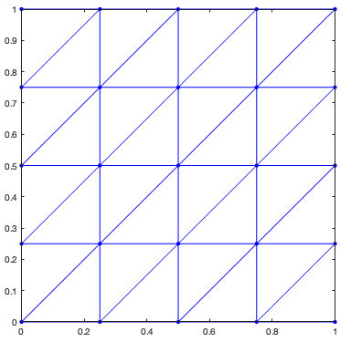
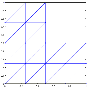
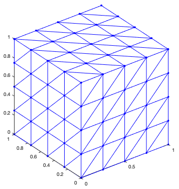
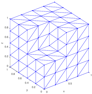
Figure 1. Coarse (level 1) triangular meshes for the unit square and the L-shape domains.

Figure 2. Coarse (level 1) tetrahedral meshes for the unit cube and the Fichera corner domains.

We assemble the mass matrices $\operatorname{M}^{\sf P1}$, $\operatorname{M}^{\sf N}$, $\operatorname{M}^{\sf RT}$ and the stiffness matrices $\operatorname{K}^{\sf P1},\operatorname{K}^{\sf N},\operatorname{K}^{\sf RT}$ defined by

$$\operatorname{M}_{ij}^{\sf P1} =\langle\theta^{\sf P1}_{i},\theta^{\sf P1}_{j}\rangle_{\mathsf{L}^{2}(\Omega)}, \operatorname{K}_{ij}^{\sf P1} =\langle\operatorname{grad}\theta^{\sf P1}_{i},\operatorname{grad}\theta^{\sf P1}_{j}\rangle_{\mathsf{L}^{2}(\Omega)},$$

$$\operatorname{M}_{ij}^{\sf N} =\langle\Theta^{\sf N}_{i},\Theta^{\sf N}_{j}\rangle_{\mathsf{L}^{2}(\Omega)}, \operatorname{K}_{ij}^{\sf N} =\langle\operatorname{curl}\Theta^{\sf N}_{i},\operatorname{curl}\Theta^{\sf N}_{j}\rangle_{\mathsf{L}^{2}(\Omega)},$$

$$\operatorname{M}_{ij}^{\sf RT} =\langle\Theta^{\sf RT}_{i},\Theta^{\sf RT}_{j}\rangle_{\mathsf{L}^{2}(\Omega)}, \operatorname{K}_{ij}^{\sf RT} =\langle\operatorname{div}\Theta^{\sf RT}_{i},\operatorname{div}\Theta^{\sf RT}_{j}\rangle_{\mathsf{L}^{2}(\Omega)},$$

where the indices $i$, $j$ are the global numbers of the corresponding degrees of freedom, i.e., they are related to mesh nodes (for P1 elements) or mesh edges or faces (for N and RT elements). By using the affine mappings (for P1 elements) or Piola mappings (for N and RT elements) from reference elements we can assemble the local matrices. Detailed implementation of finite element assemblies is explained in [1, 52]. Squares of terms from Theorem 2.17 are easy to evaluate as quadratic forms with mass and stiffness matrices:

$$|u|_{\mathsf{L}^{2}(\Omega)}^{2}= \operatorname{M}^{\sf P1}u^{\sf P1}\cdot u^{\sf P1}, |\operatorname{grad}u|_{\mathsf{L}^{2}(\Omega)}^{2} =\operatorname{K}^{\sf P1}u^{\sf P1}\cdot u^{\sf P1},$$

$$|E|_{\mathsf{L}^{2}(\Omega)}^{2}= \operatorname{M}^{\sf N}E^{\sf N}\cdot E^{\sf N}, |\operatorname{curl}E|_{\mathsf{L}^{2}(\Omega)}^{2} =\operatorname{K}^{\sf N}E^{\sf N}\cdot E^{\sf N},$$

$$|H|_{\mathsf{L}^{2}(\Omega)}^{2}= \operatorname{M}^{\sf RT}H^{\sf RT}\cdot H^{\sf RT}, |\operatorname{div}H|_{\mathsf{L}^{2}(\Omega)}^{2} =\operatorname{K}^{\sf RT}H^{\sf RT}\cdot H^{\sf RT},$$

where $u^{\sf P1}$, $E^{\sf N}$, and $H^{\sf RT}$ represent (column) vectors of coefficients with respect to their finite element bases of P1, N, and RT, respectively.

4.1. Poincaré-Friedrichs and Divergence Constants

The classical Friedrichs constant $c_{0,\Gamma}$ is approximated as

$$\frac{1}{c_{0,\Gamma,{\sf P1}}^{2}}=\lambda_{0,\Gamma,{\sf P1}}^{2}=\min_{\begin{subarray}{c}0\neq u^{\sf P1},\\ u^{\sf P1}_{\Gamma}=0\end{subarray}}\frac{\operatorname{K}^{\sf P1}u^{\sf P1}\cdot u^{\sf P1}}{\operatorname{M}^{\sf P1}u^{\sf P1}\cdot u^{\sf P1}},$$

where $u^{\sf P1}_{\Gamma}$ denotes a subvector of $u^{\sf P1}$ in indices corresponding to boundary nodes. $\lambda_{0,\Gamma,{\sf P1}}^{2}$ is the minimal (positive) eigenvalue of the generalized eigenvalue problem

$$\operatorname{K}^{\sf P1}\,u^{\sf P1}=\lambda^{2}\,\operatorname{M}^{\sf P1}\,u^{\sf P1},\qquad u^{\sf P1}_{\Gamma}=0,$$

and may also be found by computing the minimal (positive) eigenvalue of

$$\operatorname{K}^{\sf P1}_{\sf int}\,u^{\sf P1}_{\sf int}=\lambda^{2}\,\operatorname{M}^{\sf P1}_{\sf int}\,u^{\sf P1}_{\sf int},$$

where $\operatorname{K}^{\sf P1}_{\sf int}$, $\operatorname{M}^{\sf P1}_{\sf int}$, and $u^{\sf P1}_{\sf int}$ are restrictions of the matrices $\operatorname{K}^{\sf P1}$, $\operatorname{M}^{\sf P1}$, and the vector $u^{\sf P1}$, respectively, to indices corresponding to internal mesh nodes only. Note that $\operatorname{K}^{\sf P1}_{\sf int}$ is regular.

The classical Poincaré constant $c_{0,\emptyset}$ is approximated as

$$\frac{1}{c_{0,\emptyset,{\sf P1}}^{2}}=\lambda_{0,\emptyset,{\sf P1}}^{2}=\min_{\begin{subarray}{c}0\neq u^{\sf P1},\\ u^{\sf P1}\cdot 1^{\sf P1}=0\end{subarray}}\frac{\operatorname{K}^{\sf P1}u^{\sf P1}\cdot u^{\sf P1}}{\operatorname{M}^{\sf P1}u^{\sf P1}\cdot u^{\sf P1}},$$

where the constraint $u^{\sf P1}\cdot 1^{\sf P1}=0$ means that the vector $u^{\sf P1}$ has to be perpendicular to the constant vector of ones. $\lambda_{0,\emptyset,{\sf P1}}^{2}$ is the minimal positive eigenvalue of the generalized eigenvalue problem

$$\operatorname{K}^{\sf P1}\,u^{\sf P1}=\lambda^{2}\,\operatorname{M}^{\sf P1}\,u^{\sf P1}.$$

The minimal eigenvalue here is $\lambda^{2}=0$ and the corresponding eigenvector is the constant vector of ones. Analogously, the Poincaré-Friedrichs (Laplace) constants for mixed boundary conditions $c_{0,\Gamma_{\!\tau}}$ is approximated by using the same techniques and finite elements P1. More precisely, for $\Gamma_{\!\tau}\neq\emptyset$ we have

(21) $$\frac{1}{c_{0,\Gamma_{\!\tau},{\sf P1}}^{2}}=\lambda_{0,\Gamma_{\!\tau},{\sf P1}}^{2}=\min_{\begin{subarray}{c}0\neq u^{\sf P1},\\ u^{\sf P1}_{\Gamma_{\!\tau}}=0\end{subarray}}\frac{\operatorname{K}^{\sf P1}u^{\sf P1}\cdot u^{\sf P1}}{\operatorname{M}^{\sf P1}u^{\sf P1}\cdot u^{\sf P1}},$$

where $u^{\sf P1}_{\Gamma_{\!\tau}}$ denotes a subvector of $u^{\sf P1}$ in indices corresponding to boundary nodes of $\Gamma_{\!\tau}$. $\lambda_{0,\Gamma_{\!\tau},{\sf P1}}^{2}$ is the minimal (positive) eigenvalue of the generalized eigenvalue problem

$$\operatorname{K}^{\sf P1}\,u^{\sf P1}=\lambda^{2}\,\operatorname{M}^{\sf P1}\,u^{\sf P1},\qquad u^{\sf P1}_{\Gamma_{\!\tau}}=0,$$

and may be computed again by solving a restricted problem (to internal nodes and some boundary nodes) with a regular stiffness matrix $\operatorname{K}^{\sf P1}_{{\sf int},\Gamma_{\!\tau}}$, i.e.,

$$\operatorname{K}^{\sf P1}_{{\sf int},\Gamma_{\!\tau}}\,u^{\sf P1}_{{\sf int},\Gamma_{\!\tau}}=\lambda^{2}\,\operatorname{M}^{\sf P1}_{{\sf int},\Gamma_{\!\tau}}\,u^{\sf P1}_{{\sf int},\Gamma_{\!\tau}}.$$

As in any dimension the Poincaré-Friedrichs constants can be computed either as a gradient or as a divergence constant, see Theorem 2.17, we can approximate

$$c_{0,\Gamma_{\!\tau}}=c_{2,\Gamma_{\!\nu}}$$

either by (21) or by

$$\frac{1}{c_{2,\Gamma_{\!\nu},{\sf RT}}^{2}}=\lambda_{2,\Gamma_{\!\nu},{\sf RT}}^{2}=\min_{\begin{subarray}{c}0\neq H^{\sf RT},\\ H^{\sf RT}_{\Gamma_{\!\nu}}=0,\\ H^{\sf RT}\bot N(\operatorname{K}^{\sf RT})\end{subarray}}\frac{\operatorname{K}^{\sf RT}H^{\sf RT}\cdot H^{\sf RT}}{\operatorname{M}^{\sf RT}H^{\sf RT}\cdot H^{\sf RT}},$$

where $H^{\sf RT}_{\Gamma_{\!\nu}}$ denotes a subvector of $H^{\sf RT}$ in indices corresponding to boundary faces of $\Gamma_{\!\nu}$ (boundary edges in 2D). $\lambda_{2,\Gamma_{\!\nu},{\sf RT}}^{2}$ is the minimal positive eigenvalue of the generalized eigenvalue problem

$$\operatorname{K}^{\sf RT}\,H^{\sf RT}=\lambda^{2}\,\operatorname{M}^{\sf RT}\,H^{\sf RT},\qquad H^{\sf RT}_{\Gamma_{\!\nu}}=0,$$

respectively,

$$\operatorname{K}^{\sf RT}_{{\sf int},\Gamma_{\!\nu}}\,H^{\sf RT}_{{\sf int},\Gamma_{\!\nu}}=\lambda^{2}\,\operatorname{M}^{\sf RT}_{{\sf int},\Gamma_{\!\nu}}\,H^{\sf RT}_{{\sf int},\Gamma_{\!\nu}},$$

where $\operatorname{K}^{\sf RT}_{{\sf int},\Gamma_{\!\nu}}$, $\operatorname{M}^{\sf RT}_{{\sf int},\Gamma_{\!\nu}}$, and $H^{\sf RT}_{{\sf int},\Gamma_{\!\nu}}$ are restrictions of the matrices $\operatorname{K}^{\sf RT}$, $\operatorname{M}^{\sf RT}$, and the vector $H^{\sf RT}$ to indices corresponding to ‘free’ mesh faces (edges in 2D) only. Note that there are a lot of first zero eigenvalues $\lambda^{2}=0$ as neither $\operatorname{K}^{\sf RT}$ nor $\operatorname{K}^{\sf RT}_{{\sf int},\Gamma_{\!\nu}}$ are regular due to the existence of large kernels $N(\operatorname{K}^{\sf RT})$ and $N(\operatorname{K}^{\sf RT}_{{\sf int},\Gamma_{\!\nu}})$ since all rotations belong to the kernel of the divergence.

4.2. Maxwell Constants

While the computation of the Poincaré-Friedrichs constants $c_{0,\Gamma_{\!\tau}}=c_{2,\Gamma_{\!\nu}}$ is more or less independent of the dimension, the computation of the Maxwell constants is different in 2D and 3D, or generally, in ND. By Remark 3.2 (v) we have in 2D

$$c_{1,\Gamma_{\!\nu}}=c_{0,\Gamma_{\!\tau}},$$

and thus the Maxwell constants can simply be computed by the corresponding Poincaré-Friedrichs (Laplace) constants. In particular, for the tangential (electric) and normal (magnetic) Maxwell constants it holds

$$c_{1,\Gamma}=c_{0,\emptyset},\qquad c_{1,\emptyset}=c_{0,\Gamma}.$$

By Remark 3.3 (vii) we have in 3D

$$c_{1,\Gamma_{\!\tau}}=c_{1,\Gamma_{\!\nu}},$$

and thus this Maxwell constant has to be calculated separately, since the simple link to the Poincaré-Friedrichs (Laplace) constants is lost in higher dimensions. In particular, for the tangential (electric) and normal (magnetic) Maxwell constants it holds

$$c_{1,\Gamma}=c_{1,\emptyset}.$$

The Maxwell constants are approximated as

$$\frac{1}{c_{1,\Gamma_{\!\tau},{\sf N}}^{2}}=\lambda_{1,\Gamma_{\!\tau},{\sf N}}^{2}=\min_{\begin{subarray}{c}0\neq E^{\sf N},\\ E^{\sf N}_{\Gamma_{\!\tau}}=0,\\ E^{\sf N}\bot N(\operatorname{K}^{\sf N})\end{subarray}}\frac{\operatorname{K}^{\sf N}E^{\sf N}\cdot E^{\sf N}}{\operatorname{M}^{\sf N}E^{\sf N}\cdot E^{\sf N}},$$

where $E^{\sf N}_{\Gamma_{\!\tau}}$ denotes a subvector of $E^{\sf N}$ in indices corresponding to boundary edges of $\Gamma_{\!\tau}$. $\lambda_{1,\Gamma_{\!\tau},{\sf N}}^{2}$ is the minimal positive eigenvalue of the generalized eigenvalue problem

$$\operatorname{K}^{\sf N}\,E^{\sf N}=\lambda^{2}\,\operatorname{M}^{\sf N}\,E^{\sf N},\qquad E^{\sf N}_{\Gamma_{\!\tau}}=0,$$

respectively,

$$\operatorname{K}^{\sf N}_{{\sf int},\Gamma_{\!\tau}}\,E^{\sf N}_{{\sf int},\Gamma_{\!\tau}}=\lambda^{2}\,\operatorname{M}^{\sf N}_{{\sf int},\Gamma_{\!\tau}}\,E^{\sf N}_{{\sf int},\Gamma_{\!\tau}},$$

where $\operatorname{K}^{\sf N}_{{\sf int},\Gamma_{\!\tau}}$, $\operatorname{M}^{\sf N}_{{\sf int},\Gamma_{\!\tau}}$, and $E^{\sf N}_{{\sf int},\Gamma_{\!\tau}}$ are restrictions of the matrices $\operatorname{K}^{\sf N}$, $\operatorname{M}^{\sf N}$, and the vector $E^{\sf N}$ to indices corresponding to ‘free’ mesh edges only. Note that similar to the computation of the divergence constants there are a lot of first zero eigenvalues $\lambda^{2}=0$ as neither $\operatorname{K}^{\sf N}$ nor $\operatorname{K}^{\sf N}_{{\sf int},\Gamma_{\!\tau}}$ are regular due to the existence of large kernels $N(\operatorname{K}^{\sf N})$ and $N(\operatorname{K}^{\sf N}_{{\sf int},\Gamma_{\!\tau}})$ since now all gradients belong to the kernel of the rotation.

We emphasise that the Maxwell constants are also approximated by

$$\frac{1}{c_{1,\Gamma_{\!\nu},{\sf N}}^{2}}=\lambda_{1,\Gamma_{\!\nu},{\sf N}}^{2}=\min_{\begin{subarray}{c}0\neq E^{\sf N},\\ E^{\sf N}_{\Gamma_{\!\nu}}=0,\\ E^{\sf N}\bot N(\operatorname{K}^{\sf N})\end{subarray}}\frac{\operatorname{K}^{\sf N}E^{\sf N}\cdot E^{\sf N}}{\operatorname{M}^{\sf N}E^{\sf N}\cdot E^{\sf N}}.$$

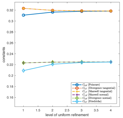
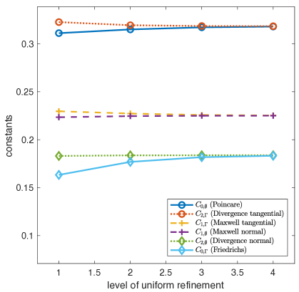
Figure 3. Constants computed for the unit square domain (left) and the unit cube domain (right) with full boundary conditions. Theoretically, it holds in 2D (left)

$$c_{0,\Gamma}=c_{2,\emptyset}=c_{1,\emptyset}=\frac{1}{\sqrt{2}\pi}\approx 0.225<c_{0,\emptyset}=c_{2,\Gamma}=c_{1,\Gamma}=\frac{1}{\pi}\approx 0.318$$

and in 3D (right)

$$c_{0,\Gamma}=c_{2,\emptyset}=\frac{1}{\sqrt{3}\pi}\approx 0.184<c_{1,\Gamma}=c_{1,\emptyset}=\frac{1}{\sqrt{2}\pi}\approx 0.225<c_{0,\emptyset}=c_{2,\Gamma}=\frac{1}{\pi}\approx 0.318.$$

4.3. 2D Computations

We demonstrate two benchmarks with the unit square and the L-shape domain, the first with known and the second with unknown values of the constants. Their coarse (level 1) meshes are displayed in Figure 2. For the unit square we have by Remark 3.2 exact values

$$c_{0,\Gamma}=c_{1,\emptyset}=\frac{1}{\sqrt{2}\pi}\approx 0.22507907,\qquad c_{0,\emptyset}=c_{1,\Gamma}=\frac{1}{\pi}\approx 0.31830988,$$

and our approximative values converge to them, see Table 4. This extends results of [54, Table 1]. For one case of mixed boundary conditions (with missing boundary part $\Gamma_{b}$) we have by Remark 3.2 and (18) exact values

$$c_{0,\Gamma_{t,l,r}}=c_{1,\Gamma_{b}}=\frac{2}{\sqrt{5}\pi}\approx 0.28470501,\qquad c_{0,\Gamma_{b}}=c_{1,\Gamma_{t,l,r}}=\frac{2}{\pi}\approx 0.63661977,$$

and our approximative values converge again to them, see Table 4. Approximative values for the L-shape domain are provided in Tables 4 and 4. We notice a quadratic convergence of all constants with respect to the mesh size $h$. It means that an absolute error of any considered constant approximation is reduced by a factor of 4 after each uniform mesh refinement. Geometrical parameters of triangular meshes used for the unit square domain are given in Table 10.

mesh level	$c_{0,\emptyset,{\sf P1}}$	$c_{2,\Gamma,{\sf RT}}$	$c_{1,\Gamma,{\sf N}}$	$c_{1,\emptyset,{\sf N}}$	$c_{2,\emptyset,{\sf RT}}$	$c_{0,\Gamma,{\sf P1}}$
1	0.31072999	0.32316745	0.32316745	0.22328039	0.22328039	0.20912552
2	0.31631302	0.31953907	0.31953907	0.22460517	0.22460517	0.22083319
3	0.31780225	0.31861815	0.31861815	0.22495907	0.22495907	0.22400032
4	0.31818232	0.31838701	0.31838701	0.22504898	0.22504898	0.22480828
5	0.31827795	0.31832917	0.31832917	0.22507155	0.22507155	0.22501131
6	0.31830190	0.31831471	0.31831471	0.22507720	0.22507720	0.22506213
7	0.31830789	0.31831109	0.31831109	0.22507861	0.22507861	0.22507484
$\infty$	0.31830988	0.31830988	0.31830988	0.22507907	0.22507907	0.22507907

Table 1. Constants computed for the unit square domain and full boundary conditions.

mesh level	$c_{0,\Gamma_{b},{\sf P1}}$	$c_{2,\Gamma_{t,l,r},{\sf RT}}$	$c_{1,\Gamma_{t,l,r},{\sf N}}$	$c_{1,\Gamma_{b},{\sf N}}$	$c_{2,\Gamma_{b},{\sf RT}}$	$c_{0,\Gamma_{t,l,r},{\sf P1}}$
1	0.63267458	0.63798842	0.63798842	0.28486798	0.28486798	0.27318834
2	0.63560893	0.63696095	0.63696095	0.28473767	0.28473767	0.28172459
3	0.63636500	0.63670501	0.63670501	0.28471277	0.28471277	0.28395286
4	0.63655592	0.63664108	0.63664108	0.28470693	0.28470693	0.28451652
5	0.63660380	0.63662510	0.63662510	0.28470549	0.28470549	0.28465786
6	0.63661578	0.63662110	0.63662110	0.28470514	0.28470514	0.28469323
7	0.63661877	0.63662011	0.63662011	0.28470505	0.28470505	0.28470207
$\infty$	0.63661977	0.63661977	0.63661977	0.28470501	0.28470501	0.28470501

Table 2. Constants computed for the unit square domain and mixed boundary conditions.

mesh level	$c_{0,\emptyset,{\sf P1}}$	$c_{2,\Gamma,{\sf RT}}$	$c_{1,\Gamma,{\sf N}}$	$c_{1,\emptyset,{\sf N}}$	$c_{2,\emptyset,{\sf RT}}$	$c_{0,\Gamma,{\sf P1}}$
1	0.39156654	0.43611331	0.43611331	0.16795692	0.16795692	0.13325394
2	0.40370423	0.42045050	0.42045050	0.16377267	0.16377267	0.15232573
3	0.40850306	0.41492017	0.41492017	0.16214127	0.16214127	0.15838355
4	0.41038725	0.41287500	0.41287500	0.16148392	0.16148392	0.16020361
5	0.41112643	0.41209870	0.41209870	0.16121879	0.16121879	0.16076463
6	0.41141712	0.41179918	0.41179918	0.16111230	0.16111230	0.16094566
7	0.41153175	0.41168242	0.41168242	0.16106970	0.16106970	0.16100698

Table 3. Constants computed for the L-shape domain and full boundary conditions.

mesh level	$c_{0,\Gamma_{b},{\sf P1}}$	$c_{2,\Gamma_{t,l,r},{\sf RT}}$	$c_{1,\Gamma_{t,l,r},{\sf N}}$	$c_{1,\Gamma_{b},{\sf N}}$	$c_{2,\Gamma_{b},{\sf RT}}$	$c_{0,\Gamma_{t,l,r},{\sf P1}}$
1	0.55287499	0.58356116	0.58356116	0.24038804	0.24038804	0.21444362
2	0.56332946	0.57483917	0.57483917	0.23765352	0.23765352	0.22916286
3	0.56716139	0.57152377	0.57152377	0.23648111	0.23648111	0.23363643
4	0.56857589	0.57025101	0.57025101	0.23597974	0.23597974	0.23498908
5	0.56910703	0.56975715	0.56975715	0.23577100	0.23577100	0.23541318
6	0.56930976	0.56956402	0.56956402	0.23568569	0.23568569	0.23555262
7	0.56938813	0.56948808	0.56948808	0.23565122	0.23565122	0.23560066

Table 4. Constants computed for the L-shape domain and mixed boundary conditions.

4.4. 3D Computations

We present two benchmarks with the unit cube and the Fichera corner domain, the first with known and the second with unknown values of the constants. Their coarse (level 1) meshes are displayed in Figure 2.

For the unit cube we have by Remark 3.3 exact values

$$c_{0,\Gamma}=\frac{1}{\sqrt{3}\pi}\approx 0.18377629,\quad c_{1,\Gamma}=c_{1,\emptyset}=\frac{1}{\sqrt{2}\pi}\approx 0.22507907,\quad c_{0,\emptyset}=\frac{1}{\pi}\approx 0.31830988,$$

and our approximative values converge to them, see Table 8. For one case of mixed boundary conditions (with missing boundary part $\Gamma_{b}$) we have by Remark 3.3 and (19), (20) exact values

$$c_{0,\Gamma_{t,l,r,f,k}}=\frac{2}{3\pi}\approx 0.21220659,\quad c_{1,\Gamma_{t,l,r,f,k}}=c_{1,\Gamma_{b}}=\frac{2}{\sqrt{5}\pi}\approx 0.28470501,\quad c_{0,\Gamma_{b}}=\frac{2}{\pi}\approx 0.63661977,$$

and our approximative values converge again to them, see Table 8. Approximative values for the Fichera corner domain are provided in Tables 8 and 8. We notice a slightly lower than quadratic convergence of all constants with respect to the mesh size $h$. Geometrical parameters of tetrahedral meshes used for the unit cube domain are given in Table 10.

mesh level	$c_{0,\emptyset,{\sf P1}}$	$c_{2,\Gamma,{\sf RT}}$	$c_{1,\Gamma,{\sf N}}$	$c_{1,\emptyset,{\sf N}}$	$c_{2,\emptyset,{\sf RT}}$	$c_{0,\Gamma,{\sf P1}}$
1	0.31114284	0.32265677	0.22964649	0.22346361	0.18305860	0.16330104
2	0.31500347	0.31939334	0.22727295	0.22461307	0.18369611	0.17685247
3	0.31720303	0.31857551	0.22577016	0.22497862	0.18375776	0.18178558
4	0.31799426	0.31837527	0.22526682	0.22505528	0.18377095	0.18324991
$\infty$	0.31830988	0.31830988	0.22507907	0.22507907	0.18377629	0.18377629

Table 5. Constants computed for the unit cube domain and full boundary conditions.

mesh level	$c_{0,\Gamma_{b},{\sf P1}}$	$c_{2,\Gamma_{t,l,r,f,k},{\sf RT}}$	$c_{1,\Gamma_{t,l,r,f,k},{\sf N}}$	$c_{1,\Gamma_{b},{\sf N}}$	$c_{2,\Gamma_{b},{\sf RT}}$	$c_{0,\Gamma_{t,l,r,f,k},{\sf P1}}$
1	0.63279353	0.63799454	0.28810408	0.28568645	0.21207495	0.19466267
2	0.63563506	0.63694323	0.28621730	0.28506833	0.21221199	0.20590030
3	0.63636820	0.63669754	0.28518535	0.28483451	0.21220585	0.21033840
4	0.63655623	0.63663874	0.28483637	0.28474355	0.21220553	0.21170560
$\infty$	0.63661977	0.63661977	0.28470501	0.28470501	0.21220659	0.21220659

Table 6. Constants computed for the unit cube domain and mixed boundary conditions.

mesh level	$c_{0,\emptyset,{\sf P1}}$	$c_{2,\Gamma,{\sf RT}}$	$c_{1,\Gamma,{\sf N}}$	$c_{1,\emptyset,{\sf N}}$	$c_{2,\emptyset,{\sf RT}}$	$c_{0,\Gamma,{\sf P1}}$
1	0.34328060	0.37118723	0.30375245	0.26905796	0.15938388	0.12490491
2	0.35193318	0.36341148	0.28961049	0.27500043	0.15638922	0.14329827
3	0.35628919	0.36072519	0.28329415	0.27728510	0.15500593	0.15042074
4	0.35808207	0.35976508	0.28054899	0.27811443	0.15444291	0.15286199

Table 7. Constants computed for the Fichera corner domain and full boundary conditions.

mesh level	$c_{0,\Gamma_{b},{\sf P1}}$	$c_{2,\Gamma_{t,l,r,f,k},{\sf RT}}$	$c_{1,\Gamma_{t,l,r,f,k},{\sf N}}$	$c_{1,\Gamma_{b},{\sf N}}$	$c_{2,\Gamma_{b},{\sf RT}}$	$c_{0,\Gamma_{t,l,r,f,k},{\sf P1}}$
1	0.59192242	0.60790729	0.32388929	0.30017867	0.19741476	0.17047720
2	0.59806507	0.60397104	0.31363043	0.30335884	0.19584527	0.18566517
3	0.60032617	0.60255178	0.30884202	0.30465706	0.19504508	0.19157456
4	0.60117716	0.60202588	0.30682949	0.30515364	0.19471006	0.19355739

Table 8. Constants computed for the Fichera corner domain and mixed boundary conditions.

4.5. Testing of the Monotonicity Properties

We perform some monotonicity tests on the constants depending on the respective boundary conditions, i.e., we display the mapping

$$\Gamma_{\!\nu}\longmapsto(c_{0,\Gamma_{\!\tau}},c_{0,\Gamma_{\!\nu}},c_{1,\Gamma_{\!\tau}},c_{1,\Gamma_{\!\nu}},c_{2,\Gamma_{\!\tau}},c_{2,\Gamma_{\!\nu}})$$

for a monotone increasing sequence of $\Gamma_{\!\nu}$. Figures 5 and 5 depict examples of such sequences in 2D/3D. The boundary part $\Gamma_{\!\nu}$ is represented discretely as a set of Neumann edges in 2D or a set of Neumann faces in 3D. Boundary faces or edges are checked for their connectivity and a breadth-first search (BFS) algorithm is applied to order them in a sequence. All constants are then evaluated for every element of the sequence and the results are displayed in Figures 7 and 7.

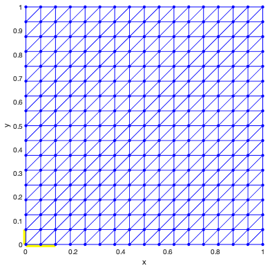
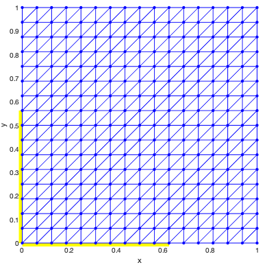
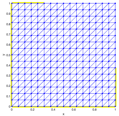
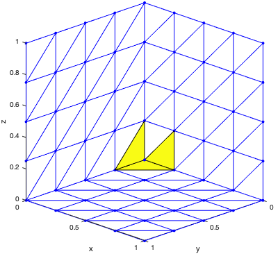
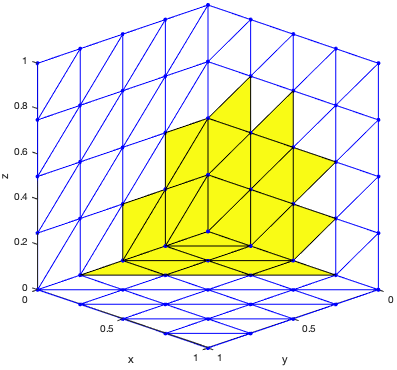
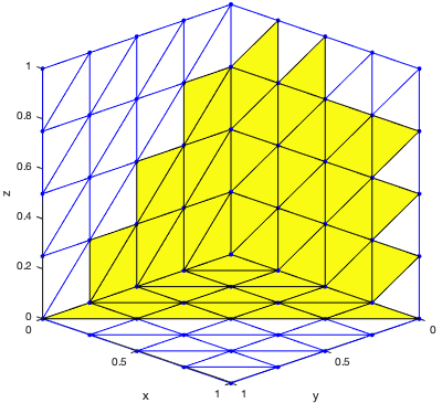
Figure 4. Elements of a monotone increasing sequence of Neumann edges $\Gamma_{\!\nu}$ with 3 (left), 7 (middle) and 19 (right) Neumann edges marked in yellow. A full boundary $\Gamma$ of the considered level 2 mesh of the unit square domain consists of 32 edges.

Figure 5. Elements of a monotone increasing sequence of Neumann faces $\Gamma_{\!\nu}$ with 3 (left), 27 (middle) and 51 (right) Neumann faces marked in yellow. A full boundary $\Gamma$ of the considered level 1 mesh of the unit cube domain consists of 192 faces.

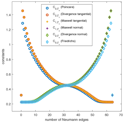
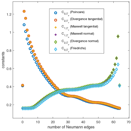
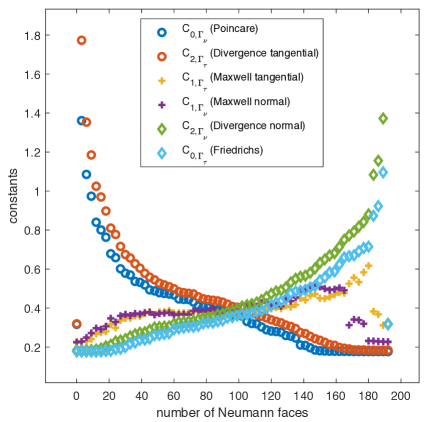
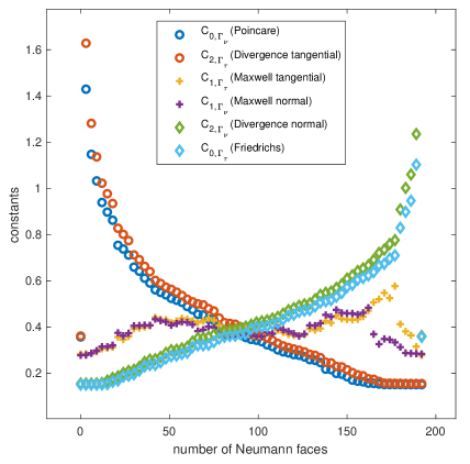
Figure 6. Constants computed for the level 3 meshes of the unit square domain (left) and of the L-shape domain (right) - monotonicity test for a monotone increasing sequence of Neumann edges $\Gamma_{\!\nu}$.

Figure 7. Constants computed for the level 1 meshes of unit cube domain (left) and of the Fichera corner domain (right) - monotonicity test for a monotone increasing sequence of Neumann faces $\Gamma_{\!\nu}$.

4.6. Computational Details and MATLAB Code

It is more computationally demanding to evaluate divergence and Maxwell constants than Laplace constants, since the numbers of faces (in 3D) and edges are higher than the number of nodes, cf. eg. Table 10 and Table 10.

A generalized eigenvalue system

(22) $$Kv=\lambda^{2}\,Mv$$

with a positive semidefinite and symmetric matrix $K\in\mathbb{R}^{n\times n}$ and a positive definite and symmetric matrix $M\in\mathbb{R}^{n\times n}$ is solved for a smallest positive eigenvalue $\lambda^{2}>0$. We apply two computational techniques.

4.6.1. A nested iteration technique

An eigenvalue evaluated on a coarser mesh (eg. by the second technique explained below) is used as initial guess on a finer (uniformly refined) mesh, where an inbuilt MATLAB function eigs is applied for the search of the closest eigenvalue. Without additional preconditioning (multigrid, domain decompositions) of eigenvalue solvers we can efficiently find smallest positive eigenvalues for all considered meshes.

However, it was noticed this technique did not converge for some cases of mixed boundary conditions in 3D because a sequence of corresponding Laplace constants did not form a monotone sequence in the monotonicity test. Then, since the dimension of the kernel of a corresponding stiffness matrix is known ($0$ or $1$), we simply compute the smallest eigenvalue or two smallest eigenvalues with 0 being the smallest eigenvalue.

4.6.2. A projection to the range of $K$

We apply the QR-decomposition of $K$ in the form

(23) $$KE=\tilde{Q}\tilde{R},$$

where $E\in\mathbb{R}^{n\times n}$ is a permutation matrix, $\tilde{Q}\in\mathbb{R}^{n\times n}$ is an orthogonal matrix and $\tilde{R}\in\mathbb{R}^{n\times n}$ is an upper triangular matrix with diagonal entries ordered in decreasing order as

$$|\tilde{R}_{1,1}|\geq\dots\geq|\tilde{R}_{r,r}|\geq\dots\geq|\tilde{R}_{n,n}|.$$

The number $r\leq n$ of nonzero entries of the sequence above then determines the range $K$ and all rows of $\tilde{R}$ with indices larger than $r$ are zero rows, cf. Figure 8 and Figure 9. Therefore, we also have

(24) $$KE=QR$$

where $Q\in\mathbb{R}^{n\times r}$ is a restriction of $\tilde{Q}$ to its first $r$ columns and $R\in\mathbb{R}^{r\times n}$ a restriction of $\tilde{R}$ to its first $r$ rows. Then, a mapping $v=Qz$ projects a (column) vector $z\in\mathbb{R}^{r}$ to the range of $K$ and the generalized eigenvalue system (22) to

$$KQz=\lambda^{2}\,MQz.$$

The multiplication of both sides by $Q^{\top}M^{-1}$ transforms the above relation (since $Q^{\top}Q$ is an identity matrix of size $r\times r$) to a standard eigenvalue problem

(25) $$Q^{\top}M^{-1}KQz=\lambda^{2}z.$$

In view of (24), the symmetry of $K$ and the orthogonality of the permutation matrix $E$, it holds

$$KQ=(QRE^{\top})Q=(QRE^{\top})^{\top}Q=ER^{\top}Q^{\top}Q=ER^{\top}$$

and this formula is applied in our practical computations. A matrix $M^{-1}$ is full and expensive to compute, its memory storage is large and the multiplication with $Q^{\top}M^{-1}$ is costly. Therefore, this projection technique can only be applied for coarser meshes.

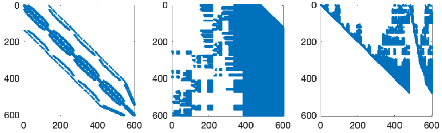
Figure 8. An example of a positive semidefinite matrix $K\in\mathbb{R}^{604\times 604}$ (left) taken as a $\operatorname{K}^{\sf N}$ matrix from level 1 mesh discretization of the unit cube domain and matrices $\tilde{Q}$ (middle) and $\tilde{R}$ (right) from the QR decomposition (23). The number of last zero rows of $\tilde{R}$ is 124 and it determines the dimension of the kernel of $K$. Therefore, the dimension of the range of $K$ is 480.

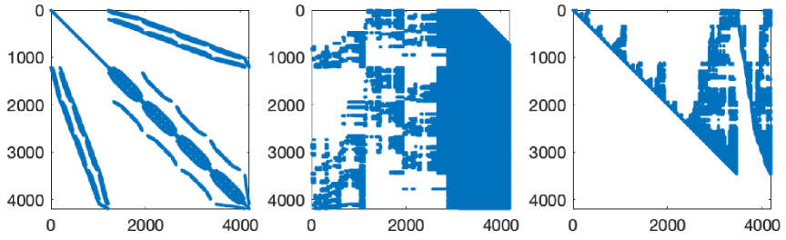
Figure 9. An example of a positive semidefinite matrix $K\in\mathbb{R}^{4184\times 4184}$ (left) taken as a $\operatorname{K}^{\sf N}$ matrix from level 2 mesh discretization of the unit cube domain and matrices $\tilde{Q}$ (middle) and $\tilde{R}$ (right) from the QR decomposition (23). The number of last zero rows of $\tilde{R}$ is 728 and it determines the dimension of the kernel of $K$. Therefore, the dimension of the range of $K$ is 3456.

mesh level	elements	nodes	edges	boundary edges
1	32	25	56	16
2	128	81	208	32
3	512	289	800	64
4	2.028	1.089	3.136	128
5	8.192	4.225	12.416	256
6	32.768	16.641	49.408	512
7	131.072	66.049	197.120	1.024

Table 9. Discretization of the unit square domain by uniform triangular meshes.

mesh level	elements	nodes	edges	faces	boundary faces
1	384	125	604	864	192
2	3.072	729	4.184	6.528	768
3	24.576	4.913	31.024	50.688	3.072
4	196.608	35.937	238.688	399.360	12.288

Table 10. Discretization of the unit cube domain by uniform tetrahedral meshes.

4.6.3. A MATLAB code

Numerical evaluations are based on finite element assemblies from [1, 52] and also utilizes a 3D cube mesh and mesh visualizations from [55]. The code is freely available for download and testing at:

https://www.mathworks.com/matlabcentral/fileexchange/23991

It can be easily modified to other domains and boundary conditions. The starting scripts for testing are start_2D and start_3D. To a given mesh, it automatically determines its boundary. In 2D, the code can also visualize eigenfunctions, see Figure 10 for the case of the L-shape domain.

5. Discussion of the Numerical Results and Conclusions

Our numerical results, especially in 3D, did verify all the theoretical assertions of Theorem 2.20, see also Remark 3.3 and Remark 3.2, in particular,

• the monotone dependence of the Poincaré-Friedrichs and divergence constants on the boundary conditions, i.e., the monotonicity of the mapping

  $$\Gamma_{\!\nu}\mapsto c_{0,\Gamma_{\!\tau}}=c_{2,\Gamma_{\!\nu}},$$

• the ‘independence’ of the Maxwell constants on the boundary conditions, i.e.,

  $$\forall\,\Gamma_{\!\tau}\subset\Gamma\qquad c_{1,\Gamma_{\!\tau}}=c_{1,\Gamma_{\!\nu}},$$

• as well as the boundedness of the full tangential and normal Maxwell constants by the Poincaré constant for convex $\Omega$, i.e.,

  $$c_{1,\Gamma}=c_{1,\emptyset}\leq c_{0,\emptyset}=c_{2,\Gamma}.$$

While the first two assertions hold for general bounded Lipschitz domains and Lipschitz interfaces, the third assertion is analytically proved only for convex domains and the full boundary conditions. In our numerical experiments, the unit cube served as a prototype for a convex domain, and we picked the Fichera corner domain as a typical example of a non-convex domain, see Figure 2 for both initial meshes.

5.1. Extended Inequalities

To our surprise, even for mixed boundary conditions and for non-convex geometries, the extended inequalities

(26) $$c_{0,\Gamma}\leq\min\{c_{0,\Gamma_{\!\tau}},c_{0,\Gamma_{\!\nu}}\}\leq c_{1,\Gamma_{\!\tau}}=c_{1,\Gamma_{\!\nu}}\leq\max\{c_{0,\Gamma_{\!\tau}},c_{0,\Gamma_{\!\nu}}\}\leq\sup_{\Gamma_{\!\tau}\neq\emptyset}c_{0,\Gamma_{\!\tau}}=\sup_{\Gamma_{\!\nu}\neq\Gamma}c_{2,\Gamma_{\!\nu}}$$

seem to hold for our examples, see Figure 7. In these special cases the Maxwell constants are always in between the Poincaré-Friedrichs (Laplace) constants. We emphasise that our examples possess (piecewise) vanishing curvature. It remains an open question if (26) is true - at least partially - in general or, e.g., for polyhedra. Moreover, if $\Gamma_{\!\tau}$ approaches $\emptyset$, the Poincaré-Friedrichs constants $c_{0,\Gamma_{\!\tau}}$ seem to be bounded, i.e., the suprema in (26) appear to be bounded, although a kernel of dimension $1$ (constants) is approximated.

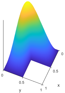
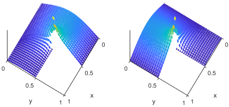
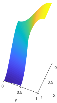
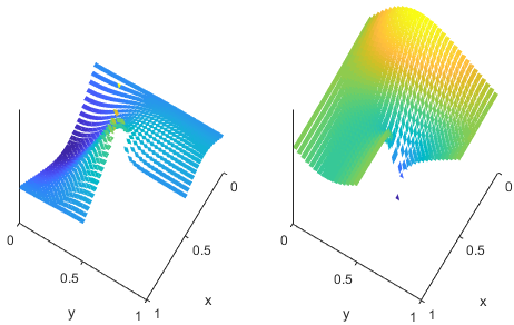
Figure 10. Eigenfunctions - Friedrichs (top left), Poincaré (bottom left), tangential Maxwell (top middle and right), normal Maxwell (bottom middle and right) - for the L-shape domain with full boundary conditions.

5.1.1. Hints for the Extended Inequalities

We note the well known integration by parts formula

(27) $$|\operatorname{grad}E|_{\mathsf{L}^{2}(\Omega)}^{2} =|\operatorname{curl}E|_{\mathsf{L}^{2}(\Omega)}^{2}+|\operatorname{div}E|_{\mathsf{L}^{2}(\Omega)}^{2},$$

being valid for all vector fields $E\in\mathsf{H}_{\Gamma}(\operatorname{grad},\Omega)$, the closure of $\Omega$-compactly supported test fields, see (15). Using a more sophisticated integration by parts formula from [12, Corollary 6], which has been proved already in, e.g., [28, Theorem 2.3] for the case of full boundary conditions, we see that (27) remains true for polyhedral domains $\Omega$ and for vector fields

(28) $$E\in\mathsf{H}_{\Gamma_{\!\tau},\Gamma_{\!\nu}}(\operatorname{grad},\Omega):=\overline{\mathsf{C}^{\infty}_{\Gamma_{\!\tau},\Gamma_{\!\nu}}(\overline{\Omega})}^{\mathsf{H}(\operatorname{grad},\Omega)}\subset\mathsf{H}(\operatorname{grad},\Omega)\cap\mathsf{H}_{\Gamma_{\!\tau}}(\operatorname{curl},\Omega)\cap\mathsf{H}_{\Gamma_{\!\nu}}(\operatorname{div},\Omega),$$

where

$$\mathsf{C}^{\infty}_{\Gamma_{\!\tau},\Gamma_{\!\nu}}(\overline{\Omega}):=\big{\{}\Phi|_{\Omega}:\Phi\in\mathsf{C}^{\infty}(\mathbb{R}^{3}),\,\text{\rm supp}\,\Phi\text{\rm compact in }\mathbb{R}^{3},\,n\times\Phi|_{\Gamma_{\!\tau}}=0,\,n\cdot\Phi|_{\Gamma_{\!\nu}}=0\big{\}}.$$

Note that these results at least go back to the book of Grisvard [31, Theorem 3.1.1.2], see also the book of Leis [36, p. 156-157].

A first hint for a possible explanation of (26) is then the following observation: Let $E_{1,\Gamma_{\!\tau}}$ be the minimiser from Remark 2.18. Then

$$E_{1,\Gamma_{\!\tau}}\in D(\operatorname{curl}_{\Gamma_{\!\tau}})\cap R(\operatorname{curl}_{\Gamma_{\!\nu}})\subset\mathsf{H}_{\Gamma_{\!\tau}}(\operatorname{curl},\Omega)\cap\mathsf{H}_{\Gamma_{\!\nu}}(\operatorname{div},\Omega),\qquad\operatorname{div}E_{1,\Gamma_{\!\tau}}=0.$$

Hence, if $\Omega$ is a polyhedron and if $E_{1,\Gamma_{\!\tau}}$ is regular enough, i.e., $E_{1,\Gamma_{\!\tau}}\in\mathsf{H}_{\Gamma_{\!\tau},\Gamma_{\!\nu}}(\operatorname{grad},\Omega)$, then by (27) and (28)

$$\lambda_{1,\Gamma_{\!\tau}} =\frac{|\operatorname{curl}E_{1,\Gamma_{\!\tau}}|_{\mathsf{L}^{2}(\Omega)}}{|E_{1,\Gamma_{\!\tau}}|_{\mathsf{L}^{2}(\Omega)}}=\frac{|\operatorname{grad}E_{1,\Gamma_{\!\tau}}|_{\mathsf{L}^{2}(\Omega)}}{|E_{1,\Gamma_{\!\tau}}|_{\mathsf{L}^{2}(\Omega)}}.$$

Moreover, if $E_{1,\Gamma_{\!\tau}}$ admits the additional regularity $E_{1,\Gamma_{\!\tau}}\in\mathsf{H}_{\Gamma_{\!\tau}}(\operatorname{grad},\Omega)$, then

$$\lambda_{1,\Gamma_{\!\tau}} \geq\inf_{0\neq E\in\mathsf{H}_{\Gamma_{\!\tau}}(\operatorname{grad},\Omega)}\frac{|\operatorname{grad}E|_{\mathsf{L}^{2}(\Omega)}}{|E|_{\mathsf{L}^{2}(\Omega)}}=\lambda_{0,\Gamma_{\!\tau}}.$$

Acknowledgment

The research of J. Valdman was supported by the Czech Science Foundation (GA R), through the grant 19-29646L. His visit in Essen in 2019 was financed by the Erasmus+ programme of the European Union.

6. Appendix: Some Proofs

Proof of (6)..

To show that, e.g., $\operatorname{A}^{*}\operatorname{A}$ is self-adjoint, we first observe that $\operatorname{A}^{*}\operatorname{A}$ is symmetric. Hence, so is $\operatorname{A}^{*}\operatorname{A}+1$. By Riesz’ representation theorem, for any $f\in\mathsf{H}_{0}$ there exists a unique $x\in D(\operatorname{A})$ such that

$$\forall\,\varphi\in D(\operatorname{A})\qquad\langle\operatorname{A}x,\operatorname{A}\varphi\rangle_{\mathsf{H}_{1}}+\langle x,\varphi\rangle_{\mathsf{H}_{0}}=\langle f,\varphi\rangle_{\mathsf{H}_{0}}.$$

Thus, $\operatorname{A}x\in D(\operatorname{A}^{*})$ and $\operatorname{A}^{*}\operatorname{A}x=f-x$, i.e., $x\in D(\operatorname{A}^{*}\operatorname{A})$ and $(\operatorname{A}^{*}\operatorname{A}+1)x=f$. In other words, $\operatorname{A}^{*}\operatorname{A}+1$ is onto. Therefore, $\operatorname{A}^{*}\operatorname{A}+1$ is self-adjoint and so is $\operatorname{A}^{*}\operatorname{A}$. Note that we did not need the additional assumption that $R(\operatorname{A})$ is closed or that $\operatorname{A}$ resp. $\operatorname{A}^{*}$ is onto.

We also present an alternative proof of the self-adjointness of $\operatorname{A}^{*}\operatorname{A}$ in the case that $R(\operatorname{A})$ is closed. For this, let $y\in\mathsf{H}_{0}$ such that there exists $z\in\mathsf{H}_{0}$ with

(29) $$\forall\,x\in D(\operatorname{A}^{*}\operatorname{A})\qquad\langle\operatorname{A}^{*}\operatorname{A}x,y\rangle_{\mathsf{H}_{0}}=\langle x,z\rangle_{\mathsf{H}_{0}}.$$

Picking $x\in N(\operatorname{A})$ shows that $z\,\bot_{\mathsf{H}_{0}}N(\operatorname{A})$, i.e., we have $z\in R(\operatorname{A}^{*})$ by (3). For $\varphi\in D(\operatorname{A}^{*})$ we note $\operatorname{A}^{*}\varphi\in R(\operatorname{A}^{*})=R(\operatorname{\mathcal{A}}^{*})$. Thus there is

$$\psi_{\varphi}:=(\operatorname{\mathcal{A}}^{*})^{-1}\operatorname{A}^{*}\varphi\in D(\operatorname{\mathcal{A}}^{*})\subset R(\operatorname{A})=R(\operatorname{\mathcal{A}})\quad\text{with}\quad\operatorname{A}^{*}\psi_{\varphi}=\operatorname{A}^{*}\varphi.$$

Moreover, there exists $x_{\varphi}:=\operatorname{\mathcal{A}}^{-1}\psi_{\varphi}\in D(\operatorname{\mathcal{A}})$ with $\operatorname{A}x_{\varphi}=\psi_{\varphi}$ and thus $x_{\varphi}\in D(\operatorname{\mathcal{A}}^{*}\operatorname{\mathcal{A}})$. By (29) we see

$$\langle\operatorname{A}^{*}\varphi,y\rangle_{\mathsf{H}_{0}} =\langle\operatorname{A}^{*}\operatorname{A}x_{\varphi},y\rangle_{\mathsf{H}_{0}}=\langle x_{\varphi},z\rangle_{\mathsf{H}_{0}}=\big{\langle}x_{\varphi},\operatorname{A}^{*}(\operatorname{\mathcal{A}}^{*})^{-1}z\big{\rangle}_{\mathsf{H}_{0}}=\big{\langle}\operatorname{A}x_{\varphi},(\operatorname{\mathcal{A}}^{*})^{-1}z\big{\rangle}_{\mathsf{H}_{1}}$$

$$=\big{\langle}\varphi,(\operatorname{\mathcal{A}}^{*})^{-1}z\big{\rangle}_{\mathsf{H}_{1}}+\underbrace{\big{\langle}\psi_{\varphi}-\varphi,(\operatorname{\mathcal{A}}^{*})^{-1}z\big{\rangle}_{\mathsf{H}_{1}}}_{=0},$$

as $\psi_{\varphi}-\varphi\in N(\operatorname{A}^{*})\,\bot_{\mathsf{H}_{1}}R(\operatorname{A})\supset D(\operatorname{\mathcal{A}}^{*})\ni(\operatorname{\mathcal{A}}^{*})^{-1}z$. Therefore, $y\in D(\operatorname{A})$ and $\operatorname{A}y=(\operatorname{\mathcal{A}}^{*})^{-1}z\in D(\operatorname{A}^{*})$, showing $y\in D(\operatorname{A}^{*}\operatorname{A})$ and $\operatorname{A}^{*}\operatorname{A}y=z$. This proves $(\operatorname{A}^{*}\operatorname{A})^{*}=\operatorname{A}^{*}\operatorname{A}$. ∎

Proof of Lemma 2.5..

We show a few selected assertions of Lemma 2.5.

$\bullet$ For an eigenvalue $\lambda>0$ and an eigenvector $(x,y)$ of $\begin{bmatrix}0&\operatorname{A}^{*}\\ \operatorname{A}&0\end{bmatrix}$ it holds $\operatorname{A}^{*}y=\lambda x$ and $\operatorname{A}x=\lambda y$. Note that $x=0$ implies $y=0$. Thus $0\neq x\in D(\operatorname{A}^{*}\operatorname{A})$ and $\operatorname{A}^{*}\operatorname{A}x=\lambda\operatorname{A}^{*}y=\lambda^{2}x$, i.e., $x$ is an eigenvector and $\lambda^{2}$ is an eigenvalue of $\operatorname{A}^{*}\operatorname{A}$.

$\bullet$ If $\lambda^{2}>0$ is an eigenvalue and $x$ is an eigenvector of $\operatorname{A}^{*}\operatorname{A}$, then $y_{\pm}:=\pm\lambda^{-1}\operatorname{A}x\in D(\operatorname{A}^{*})$ and $\operatorname{A}^{*}y_{\pm}=\pm\lambda^{-1}\operatorname{A}^{*}\operatorname{A}x=\pm\lambda x$, i.e., $(x,y_{\pm})$ is an eigenvector and $\pm\lambda$ is an eigenvalue of $\begin{bmatrix}0&\operatorname{A}^{*}\\ \operatorname{A}&0\end{bmatrix}$. Note that $y_{\pm}\neq 0$ as $y_{\pm}=0$ implies $x=0$.

$\bullet$ If $\lambda^{2}>0$ is an eigenvalue and $x$ is an eigenvector of $\operatorname{A}^{*}\operatorname{A}$, then $y:=\operatorname{A}x\in D(\operatorname{A}^{*})$ and we have $\operatorname{A}^{*}y=\operatorname{A}^{*}\operatorname{A}x=\lambda^{2}x\in D(\operatorname{A})$. Hence $y\in D(\operatorname{A}\operatorname{A}^{*})$ and $\operatorname{A}\operatorname{A}^{*}y=\lambda^{2}\operatorname{A}x=\lambda^{2}y$, i.e., $\lambda^{2}$ is an eigenvalue and $y$ is an eigenvector of $\operatorname{A}\operatorname{A}^{*}$. Note that $y\neq 0$ as $y=0$ implies $x=0$.

$\bullet$ To show that indeed, e.g., $\lambda_{\operatorname{A}}^{2}$ is the smallest positive eigenvalue of $\operatorname{A}^{*}\operatorname{A}$, let us consider a sequence $(\tilde{x}_{n})$ in $D(\operatorname{\mathcal{A}})\setminus\{0\}$ with

$$\frac{|\operatorname{A}\tilde{x}_{n}|_{\mathsf{H}_{1}}}{|\tilde{x}_{n}|_{\mathsf{H}_{0}}}\to\inf_{0\neq x\in D(\operatorname{\mathcal{A}})}\frac{|\operatorname{A}x|_{\mathsf{H}_{1}}}{|x|_{\mathsf{H}_{0}}}=\lambda_{\operatorname{A}}>0.$$

Then $(x_{n}):=(\tilde{x}_{n}/|\tilde{x}_{n}|_{\mathsf{H}_{0}})\subset D(\operatorname{\mathcal{A}})$ with $|x_{n}|_{\mathsf{H}_{0}}=1$ and

$$\lambda_{\operatorname{A}}\leq|\operatorname{A}x_{n}|_{\mathsf{H}_{1}}\to\lambda_{\operatorname{A}}.$$

Hence $(x_{n})$ is bounded in $D(\operatorname{\mathcal{A}})$, yielding a subsequence - again denoted by $(x_{n})$ - as well as $x_{\operatorname{A}}\in\mathsf{H}_{0}$ and $y_{\operatorname{A}}\in\mathsf{H}_{1}$ with $x_{n}\rightharpoonup x_{\operatorname{A}}$ in $\mathsf{H}_{0}$, $\operatorname{A}x_{n}\rightharpoonup y_{\operatorname{A}}$ in $\mathsf{H}_{1}$, and $x_{n}\to x_{\operatorname{A}}$ in $\mathsf{H}_{0}$. Then $x_{\operatorname{A}}\in D(\operatorname{A})$ and $\operatorname{A}x_{\operatorname{A}}=y_{\operatorname{A}}$ as for all $\psi\in D(\operatorname{A}^{*})$

$$\langle y_{\operatorname{A}},\psi\rangle_{\mathsf{H}_{1}}\leftarrow\langle\operatorname{A}x_{n},\psi\rangle_{\mathsf{H}_{1}}=\langle x_{n},\operatorname{A}^{*}\psi\rangle_{\mathsf{H}_{0}}\to\langle x_{\operatorname{A}},\operatorname{A}^{*}\psi\rangle_{\mathsf{H}_{0}}.$$

Note that $x_{\operatorname{A}}\in R(\operatorname{A}^{*})$ as $x_{n}\in R(\operatorname{A}^{*})=N(\operatorname{A})^{\bot_{\mathsf{H}_{0}}}$, especially, $x_{\operatorname{A}}\in D(\operatorname{\mathcal{A}})$. Moreover, $|x_{\operatorname{A}}|_{\mathsf{H}_{0}}=1$.

By elementary calculations we obtain for all $\varphi,\phi\in D(\operatorname{\mathcal{A}})$

$$\big{|}\langle\operatorname{A}\varphi,\operatorname{A}\phi\rangle_{\mathsf{H}_{1}}-\lambda_{\operatorname{A}}^{2}\langle\varphi,\phi\rangle_{\mathsf{H}_{0}}\big{|}^{2}\leq 2\big{(}|\operatorname{A}\varphi|_{\mathsf{H}_{1}}^{2}-\lambda_{\operatorname{A}}^{2}|\varphi|_{\mathsf{H}_{0}}^{2}\big{)}\big{(}|\operatorname{A}\phi|_{\mathsf{H}_{1}}^{2}-\lambda_{\operatorname{A}}^{2}|\phi|_{\mathsf{H}_{0}}^{2}\big{)}.$$

In particular, for $\varphi:=x_{n}$ we get for all $\phi\in D(\operatorname{\mathcal{A}})$

(30) $$\big{|}\langle\operatorname{A}x_{n},\operatorname{A}\phi\rangle_{\mathsf{H}_{1}}-\lambda_{\operatorname{A}}^{2}\langle x_{n},\phi\rangle_{\mathsf{H}_{0}}\big{|}^{2}\leq 2\big{(}|\operatorname{A}x_{n}|_{\mathsf{H}_{1}}^{2}-\lambda_{\operatorname{A}}^{2}\big{)}\big{(}|\operatorname{A}\phi|_{\mathsf{H}_{1}}^{2}-\lambda_{\operatorname{A}}^{2}|\phi|_{\mathsf{H}_{0}}^{2}\big{)}\to 0$$

and thus

$$\qquad\big{|}\langle\operatorname{A}x_{\operatorname{A}},\operatorname{A}\phi\rangle_{\mathsf{H}_{1}}-\lambda_{\operatorname{A}}^{2}\langle x_{\operatorname{A}},\phi\rangle_{\mathsf{H}_{0}}\big{|}$$

$$\leq\big{|}\langle\operatorname{A}(x_{\operatorname{A}}-x_{n}),\operatorname{A}\phi\rangle_{\mathsf{H}_{1}}\big{|}+\lambda_{\operatorname{A}}^{2}\big{|}\langle x_{\operatorname{A}}-x_{n},\phi\rangle_{\mathsf{H}_{0}}\big{|}+\big{|}\langle\operatorname{A}x_{n},\operatorname{A}\phi\rangle_{\mathsf{H}_{1}}-\lambda_{\operatorname{A}}^{2}\langle x_{n},\phi\rangle_{\mathsf{H}_{0}}\big{|}\to 0.$$

Hence, for all $\phi\in D(\operatorname{\mathcal{A}})$

(31) $$\langle\operatorname{A}x_{\operatorname{A}},\operatorname{A}\phi\rangle_{\mathsf{H}_{1}}=\lambda_{\operatorname{A}}^{2}\langle x_{\operatorname{A}},\phi\rangle_{\mathsf{H}_{0}}.$$

For $\phi\in D(\operatorname{A})=N(\operatorname{A})\oplus_{\mathsf{H}_{0}}D(\operatorname{\mathcal{A}})$, see the Helmholtz type decomposition (4), we decompose

$$\phi=\phi_{N}+\phi_{\operatorname{\mathcal{A}}}\in N(\operatorname{A})\oplus_{\mathsf{H}_{0}}D(\operatorname{\mathcal{A}})$$

and compute by using (31), $\operatorname{A}\phi=\operatorname{A}\phi_{\operatorname{\mathcal{A}}}$, and $x_{\operatorname{A}}\in R(\operatorname{A}^{*})\bot_{\mathsf{H}_{0}}N(\operatorname{A})$

$$\langle\operatorname{A}x_{\operatorname{A}},\operatorname{A}\phi\rangle_{\mathsf{H}_{1}}=\langle\operatorname{A}x_{\operatorname{A}},\operatorname{A}\phi_{\operatorname{\mathcal{A}}}\rangle_{\mathsf{H}_{1}}=\lambda_{\operatorname{A}}^{2}\langle x_{\operatorname{A}},\phi_{\operatorname{\mathcal{A}}}\rangle_{\mathsf{H}_{0}}=\lambda_{\operatorname{A}}^{2}\langle x_{\operatorname{A}},\phi\rangle_{\mathsf{H}_{0}}.$$

Therefore, (31) holds for all $\phi\in D(\operatorname{A})$, i.e.,

(32) $$\forall\,\phi\in D(\operatorname{A})\qquad\langle\operatorname{A}x_{\operatorname{A}},\operatorname{A}\phi\rangle_{\mathsf{H}_{1}}=\lambda_{\operatorname{A}}^{2}\langle x_{\operatorname{A}},\phi\rangle_{\mathsf{H}_{0}}.$$

This implies $\operatorname{A}x_{\operatorname{A}}\in D(\operatorname{A}^{*})$, i.e., $x_{\operatorname{A}}\in D(\operatorname{A}^{*}\operatorname{A})$ and $\operatorname{A}^{*}\operatorname{A}x_{\operatorname{A}}=\lambda_{\operatorname{A}}^{2}x_{\operatorname{A}}$. We even have $x_{\operatorname{A}}\in D(\operatorname{\mathcal{A}}^{*}\operatorname{\mathcal{A}})$. Thus, $\lambda_{\operatorname{A}}^{2}$ is an eigenvalue and $x_{\operatorname{A}}$ is an eigenvector of $\operatorname{A}^{*}\operatorname{A}$. Note that (31) or (32) implies (for $\phi=x_{\operatorname{A}}$) $|\operatorname{A}x_{\operatorname{A}}|_{\mathsf{H}_{1}}^{2}=\lambda_{\operatorname{A}}^{2}|x_{\operatorname{A}}|_{\mathsf{H}_{0}}^{2}$, i.e., $|\operatorname{A}x_{\operatorname{A}}|_{\mathsf{H}_{1}}=\lambda_{\operatorname{A}}$.

Finally, we show that $(x_{n})$ even converges strongly in $D(\operatorname{\mathcal{A}})$, i.e., $(\operatorname{A}x_{n})$ converges strongly in $\mathsf{H}_{1}$ respectively in $R(\operatorname{A})$. For this, we get for all $\phi\in D(\operatorname{\mathcal{A}})$ by (30) and (31)

$$\qquad\big{|}\langle\operatorname{A}(x_{n}-x_{\operatorname{A}}),\operatorname{A}\phi\rangle_{\mathsf{H}_{1}}-\lambda_{\operatorname{A}}^{2}\langle x_{n}-x_{\operatorname{A}},\phi\rangle_{\mathsf{H}_{0}}\big{|}^{2}$$

$$=\big{|}\langle\operatorname{A}x_{n},\operatorname{A}\phi\rangle_{\mathsf{H}_{1}}-\lambda_{\operatorname{A}}^{2}\langle x_{n},\phi\rangle_{\mathsf{H}_{0}}\big{|}^{2}\leq 2\big{(}|\operatorname{A}x_{n}|_{\mathsf{H}_{1}}^{2}-\lambda_{\operatorname{A}}^{2}\big{)}\big{(}|\operatorname{A}\phi|_{\mathsf{H}_{1}}^{2}-\lambda_{\operatorname{A}}^{2}|\phi|_{\mathsf{H}_{0}}^{2}\big{)}.$$

In particular, for $\phi=x_{n}-x_{\operatorname{A}}$ we see

$$\big{|}|\operatorname{A}(x_{n}-x_{\operatorname{A}})|_{\mathsf{H}_{1}}^{2}-\lambda_{\operatorname{A}}^{2}|x_{n}-x_{\operatorname{A}}|_{\mathsf{H}_{0}}^{2}\big{|}^{2}\leq c\big{(}|\operatorname{A}x_{n}|_{\mathsf{H}_{1}}^{2}-\lambda_{\operatorname{A}}^{2}\big{)}\to 0,$$

and hence

$$|\operatorname{A}(x_{n}-x_{\operatorname{A}})|_{\mathsf{H}_{1}}^{2}\leq\lambda_{\operatorname{A}}^{2}|x_{n}-x_{\operatorname{A}}|_{\mathsf{H}_{0}}^{2}+\big{|}|\operatorname{A}(x_{n}-x_{\operatorname{A}})|_{\mathsf{H}_{1}}^{2}-\lambda_{\operatorname{A}}^{2}|x_{n}-x_{\operatorname{A}}|_{\mathsf{H}_{0}}^{2}\big{|}\to 0.$$

$\bullet$ For $0\neq\lambda\in\sigma(\operatorname{A}^{*}\operatorname{A})$ we have $\operatorname{A}^{*}\operatorname{A}x=\lambda x$ for some $0\neq x\in D(\operatorname{A}^{*}\operatorname{A})=D(\operatorname{\mathcal{A}}^{*}\operatorname{A})$. Hence $x\in R(\operatorname{A}^{*})$ and thus $x\in D(\operatorname{\mathcal{A}})$, showing $0\neq x\in D(\operatorname{\mathcal{A}}^{*}\operatorname{\mathcal{A}})$. So $\lambda\in\sigma(\operatorname{\mathcal{A}}^{*}\operatorname{\mathcal{A}})$.

$\bullet$ For $\displaystyle 0\neq\lambda\in\sigma\Big{(}\begin{bmatrix}0&\operatorname{A}^{*}\\ \operatorname{A}&0\end{bmatrix}\Big{)}\setminus\{0\}$ we have $\operatorname{A}^{*}y=\lambda x$ and $\operatorname{A}x=\lambda y$ for some $0\neq(x,y)\in D(\operatorname{A})\times D(\operatorname{A}^{*})$. Hence $(x,y)\in R(\operatorname{A}^{*})\times R(\operatorname{A})$ and thus $(x,y)\in D(\operatorname{\mathcal{A}})\times D(\operatorname{\mathcal{A}}^{*})$, showing $0\neq(x,y)\in D(\operatorname{\mathcal{A}})\times D(\operatorname{\mathcal{A}}^{*})$. So $\displaystyle\lambda\in\sigma\Big{(}\begin{bmatrix}0&\operatorname{\mathcal{A}}^{*}\\ \operatorname{\mathcal{A}}&0\end{bmatrix}\Big{)}$.

$\bullet$ It holds

$$\big{|}\operatorname{\mathcal{A}}^{-1}\big{|}_{R(\operatorname{A}),R(\operatorname{A}^{*})}=\sup_{0\neq y\in D(\operatorname{\mathcal{A}}^{-1})}\frac{|\operatorname{\mathcal{A}}^{-1}y|_{\mathsf{H}_{0}}}{|y|_{\mathsf{H}_{1}}}=\sup_{0\neq x\in D(\operatorname{\mathcal{A}})}\frac{|x|_{\mathsf{H}_{0}}}{|\operatorname{A}x|_{\mathsf{H}_{1}}}=\Big{(}\inf_{0\neq x\in D(\operatorname{\mathcal{A}})}\frac{|\operatorname{A}x|_{\mathsf{H}_{1}}}{|x|_{\mathsf{H}_{0}}}\Big{)}^{-1}=c_{\operatorname{A}}.$$

$\bullet$ Let $x_{\operatorname{A}^{*}\operatorname{A}}$ with $|x_{\operatorname{A}^{*}\operatorname{A}}|_{\mathsf{H}_{0}}=1$ be an eigenvector of $\operatorname{A}^{*}\operatorname{A}$ to the eigenvalue $\lambda_{\operatorname{A}}^{2}$. Then $x_{\operatorname{A}^{*}\operatorname{A}}\in R(\operatorname{A}^{*})$ and $\lambda_{\operatorname{A}}^{2}(\operatorname{\mathcal{A}}^{*}\operatorname{\mathcal{A}})^{-1}x_{\operatorname{A}^{*}\operatorname{A}}=x_{\operatorname{A}^{*}\operatorname{A}}$. Thus

$$\qquad\big{|}(\operatorname{\mathcal{A}}^{*}\operatorname{\mathcal{A}})^{-1}\big{|}_{R(\operatorname{A}^{*}),R(\operatorname{A}^{*})}\leq\big{|}\operatorname{\mathcal{A}}^{-1}\big{|}_{R(\operatorname{A}),R(\operatorname{A}^{*})}\big{|}(\operatorname{\mathcal{A}}^{*})^{-1}\big{|}_{R(\operatorname{A}^{*}),R(\operatorname{A})}=c_{\operatorname{A}}^{2}$$

$$=\sup_{0\neq x\in D((\operatorname{\mathcal{A}}^{*}\operatorname{\mathcal{A}})^{-1})}\frac{\big{|}(\operatorname{\mathcal{A}}^{*}\operatorname{\mathcal{A}})^{-1}x\big{|}_{\mathsf{H}_{0}}}{|x|_{\mathsf{H}_{0}}}\geq\big{|}(\operatorname{\mathcal{A}}^{*}\operatorname{\mathcal{A}})^{-1}x_{\operatorname{A}^{*}\operatorname{A}}\big{|}_{\mathsf{H}_{0}}=\frac{1}{\lambda_{\operatorname{A}}^{2}}=c_{\operatorname{A}}^{2}.$$

$\bullet$ For $x\in N(\operatorname{A}^{*}\operatorname{A})$ we have $0=\langle\operatorname{A}^{*}\operatorname{A}x,x\rangle_{\mathsf{H}_{0}}=|\operatorname{A}x|_{\mathsf{H}_{1}}^{2}$, i.e., $x\in N(\operatorname{A})$. Analogously, we see $N(\operatorname{A}\operatorname{A}^{*})=N(\operatorname{A}^{*})$. For $x\in N(\operatorname{A}\operatorname{A}^{*}\operatorname{A})$ we have $\operatorname{A}x\in N(\operatorname{A}\operatorname{A}^{*})=N(\operatorname{A}^{*})$, i.e., $x\in N(\operatorname{A}^{*}\operatorname{A})=N(\operatorname{A})$. The latter arguments can be repeated for any higher power.

$\bullet$ For $y\in R(\operatorname{A})$ we see $x:=\operatorname{\mathcal{A}}^{-1}y\in D(\operatorname{\mathcal{A}})\subset R(\operatorname{A}^{*})$ and $z:=(\operatorname{\mathcal{A}}^{*})^{-1}x\in D(\operatorname{\mathcal{A}}^{*})\subset R(\operatorname{A})$. Thus $z\in D(\operatorname{\mathcal{A}}\operatorname{\mathcal{A}}^{*})$ and $\operatorname{A}^{*}z=x$ and $\operatorname{A}x=y$ as well as $\operatorname{A}\operatorname{A}^{*}z=\operatorname{A}x=y\in R(\operatorname{\mathcal{A}}\operatorname{\mathcal{A}}^{*})=R(\operatorname{A}\operatorname{A}^{*})$. The latter arguments can be repeated for any higher power, completing the proof. ∎

Proof of Lemma 2.11..

(i) By (6) we just have to show that $\operatorname{A}_{0}\operatorname{A}_{0}^{*}+\operatorname{A}_{1}^{*}\operatorname{A}_{1}$ is self-adjoint. For this, let $y\in\mathsf{H}_{1}$ such that there exists $z\in\mathsf{H}_{1}$ with

(33) $$\forall\,x\in D(\operatorname{A}_{0}\operatorname{A}_{0}^{*}+\operatorname{A}_{1}^{*}\operatorname{A}_{1})\qquad\big{\langle}(\operatorname{A}_{0}\operatorname{A}_{0}^{*}+\operatorname{A}_{1}^{*}\operatorname{A}_{1})x,y\big{\rangle}_{\mathsf{H}_{1}}=\langle x,z\rangle_{\mathsf{H}_{1}}.$$

Picking $x\in N_{0,1}$ shows that $z\,\bot_{\mathsf{H}_{1}}N_{0,1}$ and hence, according to Theorem 2.8, $y$ and $z$ can be orthogonally decomposed into

$$y=y_{R(\operatorname{A}_{0})}+y_{R(\operatorname{A}_{1}^{*})}+y_{N_{0,1}} \in R(\operatorname{A}_{0})\oplus_{\mathsf{H}_{1}}R(\operatorname{A}_{1}^{*})\oplus_{\mathsf{H}_{1}}N_{0,1},$$

$$z=z_{R(\operatorname{A}_{0})}+z_{R(\operatorname{A}_{1}^{*})} \in R(\operatorname{A}_{0})\oplus_{\mathsf{H}_{1}}R(\operatorname{A}_{1}^{*}).$$

(33) implies for all $x\in D(\operatorname{A}_{0}\operatorname{A}_{0}^{*}+\operatorname{A}_{1}^{*}\operatorname{A}_{1})$

(34) $$\begin{split}\langle\operatorname{A}_{0}\operatorname{A}_{0}^{*}x,y_{R(\operatorname{A}_{0})}\rangle_{\mathsf{H}_{1}}+\langle\operatorname{A}_{1}^{*}\operatorname{A}_{1}x,y_{R(\operatorname{A}_{1}^{*})}\rangle_{\mathsf{H}_{1}}&=\big{\langle}(\operatorname{A}_{0}\operatorname{A}_{0}^{*}+\operatorname{A}_{1}^{*}\operatorname{A}_{1})x,y\big{\rangle}_{\mathsf{H}_{1}}\\ &=\langle x,z\rangle_{\mathsf{H}_{1}}=\langle x,z_{R(\operatorname{A}_{0})}\rangle_{\mathsf{H}_{1}}+\langle x,z_{R(\operatorname{A}_{1}^{*})}\rangle_{\mathsf{H}_{1}}.\end{split}$$

For $x\in D(\operatorname{\mathcal{A}}_{1}^{*}\operatorname{\mathcal{A}}_{1})\subset R(\operatorname{A}_{1}^{*})\subset N(\operatorname{A}_{0}^{*})$ we see by (34) that $\langle\operatorname{A}_{1}^{*}\operatorname{A}_{1}x,y_{R(\operatorname{A}_{1}^{*})}\rangle_{\mathsf{H}_{1}}=\langle x,z_{R(\operatorname{A}_{1}^{*})}\rangle_{\mathsf{H}_{1}}$ holds, yielding by (6), i.e., $\operatorname{\mathcal{A}}_{1}^{*}\operatorname{\mathcal{A}}_{1}$ is self-adjoint, that $y_{R(\operatorname{A}_{1}^{*})}\in D(\operatorname{\mathcal{A}}_{1}^{*}\operatorname{\mathcal{A}}_{1})\subset N(\operatorname{A}_{0}^{*})$ with $\operatorname{A}_{1}^{*}\operatorname{A}_{1}y_{R(\operatorname{A}_{1}^{*})}=z_{R(\operatorname{A}_{1}^{*})}$. Analogously we see by using $x\in D(\operatorname{\mathcal{A}}_{0}\operatorname{\mathcal{A}}_{0}^{*})$ that $y_{R(\operatorname{A}_{0})}\in D(\operatorname{\mathcal{A}}_{0}\operatorname{\mathcal{A}}_{0}^{*})\subset N(\operatorname{A}_{1})$ with $\operatorname{A}_{0}\operatorname{A}_{0}^{*}y_{R(\operatorname{A}_{0})}=z_{R(\operatorname{A}_{0})}$. Thus $y\in D(\operatorname{A}_{0}\operatorname{A}_{0}^{*}+\operatorname{A}_{1}^{*}\operatorname{A}_{1})$ with $(\operatorname{A}_{0}\operatorname{A}_{0}^{*}+\operatorname{A}_{1}^{*}\operatorname{A}_{1})y=z_{R(\operatorname{A}_{0})}+z_{R(\operatorname{A}_{1}^{*})}=z$, i.e., we have shown $(\operatorname{A}_{0}\operatorname{A}_{0}^{*}+\operatorname{A}_{1}^{*}\operatorname{A}_{1})^{*}=\operatorname{A}_{0}\operatorname{A}_{0}^{*}+\operatorname{A}_{1}^{*}\operatorname{A}_{1}$.

(v) Let $0\neq\lambda\in\sigma(\operatorname{A}_{0}\operatorname{A}_{0}^{*}+\operatorname{A}_{1}^{*}\operatorname{A}_{1})$ and let $0\neq x\in D(\operatorname{A}_{0}\operatorname{A}_{0}^{*}+\operatorname{A}_{1}^{*}\operatorname{A}_{1})$ be an eigenvector to the eigenvalue $\lambda$. Then $y:=\operatorname{A}_{1}^{*}\operatorname{A}_{1}x=\lambda x-\operatorname{A}_{0}\operatorname{A}_{0}^{*}x\in D(\operatorname{A}_{1}^{*}\operatorname{A}_{1})$ and

$$\operatorname{A}_{1}^{*}\operatorname{A}_{1}y=\lambda\operatorname{A}_{1}^{*}\operatorname{A}_{1}x=\lambda y.$$

Thus, as long as $y\neq 0$, $\lambda$ is an eigenvalue of $\operatorname{A}_{1}^{*}\operatorname{A}_{1}$ with eigenvector $y$. On the other hand, if $y=0$, then $z:=\operatorname{A}_{0}\operatorname{A}_{0}^{*}x=\lambda x\in D(\operatorname{A}_{0}\operatorname{A}_{0}^{*})\setminus\{0\}$ and $\operatorname{A}_{0}\operatorname{A}_{0}^{*}z=\lambda\operatorname{A}_{0}\operatorname{A}_{0}^{*}x=\lambda z$. Hence $\lambda$ is an eigenvalue of $\operatorname{A}_{0}\operatorname{A}_{0}^{*}$ with eigenvector $z$. This shows

$$\sigma(\operatorname{A}_{0}\operatorname{A}_{0}^{*}+\operatorname{A}_{1}^{*}\operatorname{A}_{1})\setminus\{0\}\subset\big{(}\sigma(\operatorname{A}_{0}\operatorname{A}_{0}^{*})\setminus\{0\}\big{)}\cup\big{(}\sigma(\operatorname{A}_{1}^{*}\operatorname{A}_{1})\setminus\{0\}\big{)}.$$

For the other inclusion, let, e.g., $0\neq\lambda\in\sigma(\operatorname{A}_{1}^{*}\operatorname{A}_{1})$ and let $0\neq x\in D(\operatorname{A}_{1}^{*}\operatorname{A}_{1})$ be an eigenvector to the eigenvalue $\lambda$. Then $x\in R(\operatorname{A}_{1}^{*})\subset N(\operatorname{A}_{0}^{*})$ and thus $(\operatorname{A}_{0}\operatorname{A}_{0}^{*}+\operatorname{A}_{1}^{*}\operatorname{A}_{1})x=\operatorname{A}_{1}^{*}\operatorname{A}_{1}x=\lambda x$, i.e., $\lambda$ is an eigenvalue of $\operatorname{A}_{0}\operatorname{A}_{0}^{*}+\operatorname{A}_{1}^{*}\operatorname{A}_{1}$ with eigenvector $x$. Thus

$$\sigma(\operatorname{A}_{1}^{*}\operatorname{A}_{1})\setminus\{0\}\subset\sigma(\operatorname{A}_{0}\operatorname{A}_{0}^{*}+\operatorname{A}_{1}^{*}\operatorname{A}_{1})\setminus\{0\},$$

and analogously we show $\sigma(\operatorname{A}_{0}\operatorname{A}_{0}^{*})\setminus\{0\}\subset\sigma(\operatorname{A}_{0}\operatorname{A}_{0}^{*}+\operatorname{A}_{1}^{*}\operatorname{A}_{1})\setminus\{0\}$.

(iii) Let $x\in N(\operatorname{A}_{0}\operatorname{A}_{0}^{*}+\operatorname{A}_{1}^{*}\operatorname{A}_{1})$. Then

$$0=\big{\langle}(\operatorname{A}_{0}\operatorname{A}_{0}^{*}+\operatorname{A}_{1}^{*}\operatorname{A}_{1})x,x\big{\rangle}_{\mathsf{H}_{1}}=|\operatorname{A}_{0}^{*}x|_{\mathsf{H}_{0}}^{2}+|\operatorname{A}_{1}x|_{\mathsf{H}_{2}}^{2},$$

showing $x\in N_{0,1}$. As $D(\operatorname{A}_{1})\cap D(\operatorname{A}_{0}^{*})\hookrightarrow\mathsf{H}_{1}$ is compact, so is $D(\operatorname{A}_{0}\operatorname{A}_{0}^{*}+\operatorname{A}_{1}^{*}\operatorname{A}_{1})\hookrightarrow\mathsf{H}_{1}$, showing that the range $R(\operatorname{A}_{0}\operatorname{A}_{0}^{*}+\operatorname{A}_{1}^{*}\operatorname{A}_{1})$ is closed by Remark 2.3 (ii). Thus

$$R(\operatorname{A}_{0}\operatorname{A}_{0}^{*}+\operatorname{A}_{1}^{*}\operatorname{A}_{1})=N(\operatorname{A}_{0}\operatorname{A}_{0}^{*}+\operatorname{A}_{1}^{*}\operatorname{A}_{1})^{\bot_{\mathsf{H}_{1}}}=N_{0,1}^{\bot_{\mathsf{H}_{1}}},$$

finishing the proof. ∎

7. Appendix: Analytical Calculations

We compute the exact eigenvalues and eigenfunctions of Section 3 in detail.

7.1. 1D

Recall the situation and notations from Section 2.3.1 and Section 3.1. In particular,

$$\frac{1}{c_{0,\Gamma_{\!\tau}}}=\lambda_{0,\Gamma_{\!\tau}}=\lambda_{0,\Gamma_{\!\nu}}=\frac{1}{c_{0,\Gamma_{\!\nu}}}.$$

Let $u=u_{0,\Gamma_{\!\tau}}$ be the first eigenfunction for the eigenvalue $\lambda^{2}$ with $\lambda=\lambda_{0,\Gamma_{\!\tau}}>0$ of $-\Delta_{\Gamma_{\!\tau}}$. Hence, we have $E_{0,\Gamma_{\!\nu}}=\operatorname{grad}u_{0,\Gamma_{\!\tau}}$ and

$$u\in D(\Delta_{\Gamma_{\!\tau}})\cap\mathsf{L}^{2}_{\Gamma_{\!\nu}}(\Omega)\subset\mathsf{H}^{1}_{\Gamma_{\!\tau}}(\Omega)\cap\mathsf{L}^{2}_{\Gamma_{\!\nu}}(\Omega),\qquad\operatorname{grad}u=u^{\prime}\in D(\operatorname{div}_{\Gamma_{\!\nu}})=\mathsf{H}^{1}_{\Gamma_{\!\nu}}(\Omega),$$

as well as

$$(-\Delta-\lambda^{2})u=-u^{\prime\prime}-\lambda^{2}u=0.$$

Then

$$u=\alpha\sin(\lambda x)+\beta\cos(\lambda x),\qquad u^{\prime}(x)=\alpha\lambda\cos(\lambda x)-\beta\lambda\sin(\lambda x).$$

For the different boundary conditions we get:

$\bullet$ $\Gamma_{\!\tau}=\emptyset$ and $\Gamma_{\!\nu}=\Gamma$, i.e., $u^{\prime}(0)=u^{\prime}(1)=0$: $\alpha=0$, $\lambda=n\pi$, $n\in\mathbb{N}_{0}$, i.e.,

$$\lambda_{0,\emptyset}=\pi,\qquad u_{0,\emptyset}(x)=\beta\cos(\pi x).$$

Note that in this case the first eigenvalue is $\lambda=0$.

$\bullet$ $\Gamma_{\!\tau}=\{0\}$ and $\Gamma_{\!\nu}=\{1\}$, i.e., $u(0)=u^{\prime}(1)=0$: $\beta=0$, $\lambda=(n-1/2)\pi$, $n\in\mathbb{N}$, i.e.,

$$\lambda_{0,\{0\}}=\frac{\pi}{2},\qquad u_{0,\{0\}}(x)=\alpha\sin(\frac{\pi}{2}x).$$

$\bullet$ $\Gamma_{\!\tau}=\{1\}$ and $\Gamma_{\!\nu}=\{0\}$, i.e., $u^{\prime}(0)=u(1)=0$: $\alpha=0$, $\lambda=(n-1/2)\pi$, $n\in\mathbb{N}$, i.e.,

$$\lambda_{0,\{1\}}=\frac{\pi}{2},\qquad u_{0,\{1\}}(x)=\beta\cos(\frac{\pi}{2}x).$$

$\bullet$ $\Gamma_{\!\tau}=\Gamma$ and $\Gamma_{\!\nu}=\emptyset$, i.e., $u(0)=u(1)=0$: $\beta=0$, $\lambda=n\pi$, $n\in\mathbb{N}$, i.e.,

$$\lambda_{0,\Gamma}=\pi,\qquad u_{0,\Gamma}(x)=\alpha\sin(\pi x).$$

Note that from $\lambda_{0,\Gamma_{\!\tau}}=\lambda_{0,\Gamma_{\!\nu}}$ we already know $\lambda_{0,\Gamma}=\lambda_{0,\emptyset}$ and $\lambda_{0,\{0\}}=\lambda_{0,\{1\}}$, i.e.,

$$\lambda_{0,\Gamma}=\lambda_{0,\emptyset}=\pi,\qquad\lambda_{0,\{0\}}=\lambda_{0,\{1\}}=\frac{\pi}{2}.$$

7.2. 2D

Recall the situation and notations from Section 2.3.2 and Section 3.2. In particular,

$$\frac{1}{c_{0,\Gamma_{\!\tau}}}=\lambda_{0,\Gamma_{\!\tau}}=\lambda_{1,\Gamma_{\!\nu}}=\frac{1}{c_{1,\Gamma_{\!\nu}}}.$$

Let $u=u_{0,\Gamma_{\!\tau}}$ be the first eigenfunction for the eigenvalue $\lambda^{2}$ with $\lambda=\lambda_{0,\Gamma_{\!\tau}}>0$ of $-\Delta_{\Gamma_{\!\tau}}$. Hence, we have $E_{0,\Gamma_{\!\nu}}=\operatorname{grad}u_{0,\Gamma_{\!\tau}}$ and

$$u\in D(\Delta_{\Gamma_{\!\tau}})\cap\mathsf{L}^{2}_{\Gamma_{\!\nu}}(\Omega)\subset\mathsf{H}^{1}_{\Gamma_{\!\tau}}(\Omega)\cap\mathsf{L}^{2}_{\Gamma_{\!\nu}}(\Omega),\qquad\operatorname{grad}u\in D(\operatorname{div}_{\Gamma_{\!\nu}})=\mathsf{H}_{\Gamma_{\!\nu}}(\operatorname{div},\Omega),$$

as well as

$$(-\Delta-\lambda^{2})u=0.$$

Separation of variables shows with $u(x)=u_{1}(x_{1})u_{2}(x_{2})$ and $\operatorname{grad}u(x)=\begin{bmatrix}u_{1}^{\prime}(x_{1})u_{2}(x_{2})\\ u_{1}(x_{1})u_{2}^{\prime}(x_{2})\end{bmatrix}$

$$0=(-\Delta-\lambda^{2})u(x)=-u_{1}^{\prime\prime}(x_{1})u_{2}(x_{2})-u_{1}(x_{1})u_{2}^{\prime\prime}(x_{2})-\lambda^{2}u_{1}(x_{1})u_{2}(x_{2}).$$

For fixed $x_{2}$ with $u_{2}(x_{2})\neq 0$ we get

$$-u_{1}^{\prime\prime}(x_{1})-\mu_{1}^{2}u_{1}(x_{1})=0,\qquad\mu_{1}^{2}=\frac{u_{2}^{\prime\prime}(x_{2})}{u_{2}(x_{2})}+\lambda^{2},$$

i.e.,

$$-u_{1}^{\prime\prime}(x_{1})-\mu_{1}^{2}u_{1}(x_{1})=0,\quad-u_{2}^{\prime\prime}(x_{2})-\mu_{2}^{2}u_{2}(x_{2})=0,\quad\lambda^{2}=\mu_{1}^{2}+\mu_{2}^{2}.$$

The Dirichlet boundary conditions, i.e.,

$$u=0\quad\text{on}\quad\Gamma_{\!\tau},$$

reduce to Dirichlet boundary conditions for $u_{1}$ and $u_{2}$, respectively, and the Neumann boundary conditions, i.e.,

$$n\cdot\operatorname{grad}u=0\quad\text{on}\quad\Gamma_{\!\nu},$$

reduce to Dirichlet boundary conditions for $u_{1}^{\prime}$ and $u_{2}^{\prime}$, respectively. More precisely, we have:

$\bullet$ $\Gamma_{l}$, $n=-e^{1}$, $x_{1}=0$:

$$0=u|_{\Gamma_{l}} =u_{1}u_{2}|_{\Gamma_{l}} \Rightarrow u_{1}(0) =0,$$

$$0=n\cdot\operatorname{grad}u|_{\Gamma_{l}} =-u_{1}^{\prime}u_{2}|_{\Gamma_{l}} \Rightarrow u_{1}^{\prime}(0) =0.$$

$\bullet$ $\Gamma_{r}$, $n=e^{1}$, $x_{1}=1$:

$$0=u|_{\Gamma_{r}} =u_{1}u_{2}|_{\Gamma_{r}} \Rightarrow u_{1}(1) =0,$$

$$0=n\cdot\operatorname{grad}u|_{\Gamma_{r}} =u_{1}^{\prime}u_{2}|_{\Gamma_{r}} \Rightarrow u_{1}^{\prime}(1) =0.$$

$\bullet$ $\Gamma_{b}$, $n=-e^{2}$, $x_{2}=0$:

$$0=u|_{\Gamma_{b}} =u_{1}u_{2}|_{\Gamma_{b}} \Rightarrow u_{2}(0) =0,$$

$$0=n\cdot\operatorname{grad}u|_{\Gamma_{b}} =-u_{1}u_{2}^{\prime}|_{\Gamma_{b}} \Rightarrow u_{2}^{\prime}(0) =0.$$

$\bullet$ $\Gamma_{t}$, $n=e^{2}$, $x_{2}=1$:

$$0=u|_{\Gamma_{t}} =u_{1}u_{2}|_{\Gamma_{t}} \Rightarrow u_{2}(1) =0,$$

$$0=n\cdot\operatorname{grad}u|_{\Gamma_{t}} =u_{1}u_{2}^{\prime}|_{\Gamma_{t}} \Rightarrow u_{2}^{\prime}(1) =0.$$

The 1D case shows for the different boundary conditions the following:

$\bullet$ $\Gamma_{\!\tau}=\emptyset$ and $\Gamma_{\!\nu}=\Gamma$, i.e., $u_{1}^{\prime}(0)=u_{1}^{\prime}(1)=u_{2}^{\prime}(0)=u_{2}^{\prime}(1)=0$: $\mu_{1}=n\pi$, $\mu_{2}=m\pi$, i.e., $\lambda=\sqrt{n^{2}+m^{2}}\pi$, $n,m\in\mathbb{N}_{0}$, and

$$\lambda_{0,\emptyset}=\pi,\qquad u_{0,\emptyset}(x)=\alpha\cos(\pi x_{1})+\beta\cos(\pi x_{2}).$$

Note that in this case the first eigenvalue is $\lambda=0$.

$\bullet$ $\Gamma_{\!\tau}=\Gamma_{b}$ and $\Gamma_{\!\nu}=\Gamma_{t,l,r}$, i.e., $u_{1}^{\prime}(0)=u_{1}^{\prime}(1)=u_{2}(0)=u_{2}^{\prime}(1)=0$: $\mu_{1}=n\pi$, $\mu_{2}=(m-1/2)\pi$, i.e., $\lambda=\sqrt{n^{2}+(m-1/2)^{2}}\pi$, $n\in\mathbb{N}_{0}$, $m\in\mathbb{N}$, and

$$\lambda_{0,\Gamma_{b}}=\frac{1}{2}\pi,\qquad u_{0,\Gamma_{b}}(x)=\alpha\sin(\frac{\pi}{2}x_{2}).$$

$\bullet$ $\Gamma_{\!\tau}=\Gamma_{b,t}$ and $\Gamma_{\!\nu}=\Gamma_{l,r}$, i.e., $u_{1}^{\prime}(0)=u_{1}^{\prime}(1)=u_{2}(0)=u_{2}(1)=0$: $\mu_{1}=n\pi$, $\mu_{2}=m\pi$, i.e., $\lambda=\sqrt{n^{2}+m^{2}}\pi$, $n\in\mathbb{N}_{0}$, $m\in\mathbb{N}$, and

$$\lambda_{0,\Gamma_{b,t}}=\pi,\qquad u_{0,\Gamma_{b,t}}(x)=\alpha\sin(\pi x_{2}).$$

$\bullet$ $\Gamma_{\!\tau}=\Gamma_{b,l}$ and $\Gamma_{\!\nu}=\Gamma_{t,r}$, i.e., $u_{1}(0)=u_{1}^{\prime}(1)=u_{2}(0)=u_{2}^{\prime}(1)=0$: $\mu_{1}=(n-1/2)\pi$, $\mu_{2}=(m-1/2)\pi$, i.e., $\lambda=\sqrt{(n-1/2)^{2}+(m-1/2)^{2}}\pi$, $n,m\in\mathbb{N}$, and

$$\lambda_{0,\Gamma_{b,l}}=\frac{\sqrt{2}}{2}\pi,\qquad u_{0,\Gamma_{b,l}}(x)=\alpha\sin(\frac{\pi}{2}x_{1})\sin(\frac{\pi}{2}x_{2}).$$

$\bullet$ $\Gamma_{\!\tau}=\Gamma_{b,l,r}$ and $\Gamma_{\!\nu}=\Gamma_{t}$, i.e., $u_{1}(0)=u_{1}(1)=u_{2}(0)=u_{2}^{\prime}(1)=0$: $\mu_{1}=n\pi$, $\mu_{2}=(m-1/2)\pi$, i.e., $\lambda=\sqrt{n^{2}+(m-1/2)^{2}}\pi$, $n,m\in\mathbb{N}$, and

$$\lambda_{0,\Gamma_{b,l,r}}=\frac{\sqrt{5}}{2}\pi,\qquad u_{0,\Gamma_{b,l,r}}(x)=\alpha\sin(\pi x_{1})\sin(\frac{\pi}{2}x_{2}).$$

$\bullet$ $\Gamma_{\!\tau}=\Gamma$ and $\Gamma_{\!\nu}=\emptyset$, i.e., $u_{1}(0)=u_{1}(1)=u_{2}(0)=u_{2}(1)=0$: $\mu_{1}=n\pi$, $\mu_{2}=m\pi$, i.e., $\lambda=\sqrt{n^{2}+m^{2}}\pi$, $n,m\in\mathbb{N}$, and

$$\lambda_{0,\Gamma}=\sqrt{2}\pi,\qquad u_{0,\Gamma}(x)=\alpha\sin(\pi x_{1})\sin(\pi x_{2}).$$

All other cases follow by symmetry, i.e.,

$$\lambda_{0,\emptyset} =\pi, \lambda_{0,\Gamma_{b,l}}=\lambda_{0,\Gamma_{b,r}}=\lambda_{0,\Gamma_{t,l}}=\lambda_{0,\Gamma_{t,r}} =\frac{\sqrt{2}}{2}\pi,$$

$$\lambda_{0,\Gamma_{b}}=\lambda_{0,\Gamma_{t}}=\lambda_{0,\Gamma_{l}}=\lambda_{0,\Gamma_{r}} =\frac{1}{2}\pi, \lambda_{0,\Gamma_{b,l,r}}=\lambda_{0,\Gamma_{t,l,r}}=\lambda_{0,\Gamma_{b,t,l}}=\lambda_{0,\Gamma_{b,t,r}} =\frac{\sqrt{5}}{2}\pi,$$

$$\lambda_{0,\Gamma_{b,t}}=\lambda_{0,\Gamma_{l,r}} =\pi, \lambda_{0,\Gamma} =\sqrt{2}\pi.$$

7.3. 3D

Recall the situation and notations from Section 2.2, Theorem 2.20, and Section 3.3. In particular,

$$\frac{1}{c_{0,\Gamma_{\!\tau}}}=\lambda_{0,\Gamma_{\!\tau}}=\lambda_{2,\Gamma_{\!\nu}}=\frac{1}{c_{2,\Gamma_{\!\nu}}},\qquad\frac{1}{c_{1,\Gamma_{\!\tau}}}=\lambda_{1,\Gamma_{\!\tau}}=\lambda_{1,\Gamma_{\!\nu}}=\frac{1}{c_{1,\Gamma_{\!\nu}}}.$$

Let $u=u_{0,\Gamma_{\!\tau}}$ be the first eigenfunction for the eigenvalue $\lambda^{2}$ with $\lambda=\lambda_{0,\Gamma_{\!\tau}}>0$ of $-\Delta_{\Gamma_{\!\tau}}$. Analogously, let $E=E_{1,\Gamma_{\!\tau}}$ be the first eigenfunction for the eigenvalue $\widetilde{\lambda}^{2}$ with $\widetilde{\lambda}=\lambda_{1,\Gamma_{\!\tau}}>0$ of $\square_{\Gamma_{\!\tau}}$. Hence,

$$u \in D(\Delta_{\Gamma_{\!\tau}})\cap\mathsf{L}^{2}_{\Gamma_{\!\nu}}(\Omega)\subset\mathsf{H}^{1}_{\Gamma_{\!\tau}}(\Omega)\cap\mathsf{L}^{2}_{\Gamma_{\!\nu}}(\Omega), E \in D(\square_{\Gamma_{\!\tau}})\cap R(\operatorname{curl}_{\Gamma_{\!\nu}})\subset\mathsf{H}_{\Gamma_{\!\tau}}(\operatorname{curl},\Omega)\cap R(\operatorname{curl}_{\Gamma_{\!\nu}}),$$

$$\operatorname{grad}u \in D(\operatorname{div}_{\Gamma_{\!\nu}})=\mathsf{H}_{\Gamma_{\!\nu}}(\operatorname{div},\Omega), \operatorname{curl}E \in D(\operatorname{curl}_{\Gamma_{\!\nu}})\cap R(\operatorname{curl}_{\Gamma_{\!\tau}})=\mathsf{H}_{\Gamma_{\!\nu}}(\operatorname{curl},\Omega)\cap R(\operatorname{curl}_{\Gamma_{\!\tau}}),$$

and we have by $-\Delta=\operatorname{curl}\operatorname{curl}-\operatorname{grad}\operatorname{div}=\square-\operatorname{grad}\operatorname{div}$

$$(-\Delta-\lambda^{2})u=0,\qquad(-\Delta-\widetilde{\lambda}^{2})E=(\square-\widetilde{\lambda}^{2})E=0,$$

as $\operatorname{div}E=0$. Let us first discuss $u$. Separation of variables shows with

$$u(x)=\widehat{u}(\widehat{x})u_{3}(x_{3})=u_{1}(x_{1})u_{2}(x_{2})u_{3}(x_{3}),\quad\widehat{u}(\widehat{x})=u_{1}(x_{1})u_{2}(x_{2}),\qquad x=\begin{bmatrix}\widehat{x}\\ x_{3}\end{bmatrix},\quad\widehat{x}=\begin{bmatrix}x_{1}\\ x_{2}\end{bmatrix}$$

and

$$\operatorname{grad}u(x)=\begin{bmatrix}u_{3}(x_{3})\operatorname{grad}\widehat{u}(\widehat{x})\\ u_{3}^{\prime}(x_{3})\widehat{u}(\widehat{x})\end{bmatrix}=\begin{bmatrix}u_{1}^{\prime}(x_{1})u_{2}(x_{2})u_{3}(x_{3})\\ u_{1}(x_{1})u_{2}^{\prime}(x_{2})u_{3}(x_{3})\\ u_{1}(x_{1})u_{2}(x_{2})u_{3}^{\prime}(x_{3})\end{bmatrix},\quad\operatorname{grad}\widehat{u}(\widehat{x})=\begin{bmatrix}u_{1}^{\prime}(x_{1})u_{2}(x_{2})\\ u_{1}(x_{1})u_{2}^{\prime}(x_{2})\end{bmatrix}$$

that

$$0=(-\Delta-\lambda^{2})u(x)=-\Delta\widehat{u}(\widehat{x})u_{3}(x_{3})-\widehat{u}(\widehat{x})u_{3}^{\prime\prime}(x_{3})-\lambda^{2}\widehat{u}(\widehat{x})u_{3}(x_{3}).$$

For fixed $x_{3}$ with $u_{3}(x_{3})\neq 0$ we get

$$-\Delta\widehat{u}(\widehat{x})-\widehat{\mu}^{2}\widehat{u}(\widehat{x})=0,\qquad\widehat{\mu}^{2}=\frac{u_{3}^{\prime\prime}(x_{3})}{u_{3}(x_{3})}+\lambda^{2},$$

i.e.,

$$-\Delta\widehat{u}(\widehat{x})-\widehat{\mu}^{2}\widehat{u}(\widehat{x})=0,\quad-u_{3}^{\prime\prime}(x_{3})-\mu_{3}^{2}u_{3}(x_{3})=0,\quad\lambda^{2}=\widehat{\mu}^{2}+\mu_{3}^{2}.$$

From the 2D case we already know $\widehat{\mu}^{2}=\mu_{1}^{2}+\mu_{2}^{2}$ and the splitting of $\widehat{u}$, i.e.,

$$\lambda^{2}=\mu_{1}^{2}+\mu_{2}^{2}+\mu_{3}^{2}$$

and

$$-u_{1}^{\prime\prime}(x_{1})-\mu_{1}^{2}u_{1}(x_{1})=0,\quad-u_{2}^{\prime\prime}(x_{2})-\mu_{2}^{2}u_{2}(x_{2})=0,\quad-u_{3}^{\prime\prime}(x_{3})-\mu_{3}^{2}u_{3}(x_{3})=0.$$

The Dirichlet boundary conditions, i.e.,

$$u=0\quad\text{on}\quad\Gamma_{\!\tau},$$

reduce to Dirichlet boundary conditions for $u_{1}$, $u_{2}$, and $u_{3}$, respectively, and the Neumann boundary conditions, i.e.,

$$n\cdot\operatorname{grad}u=0\quad\text{on}\quad\Gamma_{\!\nu},$$

reduce to Neumann boundary conditions for $\widehat{u}$ and $u_{3}$ and hence to Dirichlet boundary conditions for $u_{1}^{\prime}$, $u_{2}^{\prime}$, and $u_{3}^{\prime}$, respectively.

$\bullet$ $\Gamma_{k}$, $n=-e^{1}$, $x_{1}=0$:

$$0=u|_{\Gamma_{k}} =u_{1}u_{2}u_{3}|_{\Gamma_{k}} \Rightarrow u_{1}(0) =0,$$

$$0=n\cdot\operatorname{grad}u|_{\Gamma_{k}} =-u_{1}^{\prime}u_{2}u_{3}|_{\Gamma_{k}} \Rightarrow u_{1}^{\prime}(0) =0.$$

$\bullet$ $\Gamma_{f}$, $n=e^{1}$, $x_{1}=1$:

$$0=u|_{\Gamma_{f}} =u_{1}u_{2}u_{3}|_{\Gamma_{f}} \Rightarrow u_{1}(1) =0,$$

$$0=n\cdot\operatorname{grad}u|_{\Gamma_{f}} =u_{1}^{\prime}u_{2}u_{3}|_{\Gamma_{f}} \Rightarrow u_{1}^{\prime}(1) =0.$$

$\bullet$ $\Gamma_{l}$, $n=-e^{2}$, $x_{2}=0$:

$$0=u|_{\Gamma_{l}} =u_{1}u_{2}u_{3}|_{\Gamma_{l}} \Rightarrow u_{2}(0) =0,$$

$$0=n\cdot\operatorname{grad}u|_{\Gamma_{l}} =-u_{1}u_{2}^{\prime}u_{3}|_{\Gamma_{l}} \Rightarrow u_{2}^{\prime}(0) =0.$$

$\bullet$ $\Gamma_{r}$, $n=e^{2}$, $x_{2}=1$:

$$0=u|_{\Gamma_{r}} =u_{1}u_{2}u_{3}|_{\Gamma_{r}} \Rightarrow u_{2}(1) =0,$$

$$0=n\cdot\operatorname{grad}u|_{\Gamma_{r}} =u_{1}u_{2}^{\prime}u_{3}|_{\Gamma_{r}} \Rightarrow u_{2}^{\prime}(1) =0.$$

$\bullet$ $\Gamma_{b}$, $n=-e^{3}$, $x_{3}=0$:

$$0=u|_{\Gamma_{b}} =u_{1}u_{2}u_{3}|_{\Gamma_{b}} \Rightarrow u_{3}(0) =0,$$

$$0=n\cdot\operatorname{grad}u|_{\Gamma_{b}} =-u_{1}u_{2}u_{3}^{\prime}|_{\Gamma_{b}} \Rightarrow u_{3}^{\prime}(0) =0.$$

$\bullet$ $\Gamma_{t}$, $n=e^{3}$, $x_{3}=1$:

$$0=u|_{\Gamma_{t}} =u_{1}u_{2}u_{3}|_{\Gamma_{t}} \Rightarrow u_{3}(1) =0,$$

$$0=n\cdot\operatorname{grad}u|_{\Gamma_{t}} =u_{1}u_{2}u_{3}^{\prime}|_{\Gamma_{t}} \Rightarrow u_{3}^{\prime}(1) =0.$$

The 1D case shows for the different boundary conditions the following:

$\bullet$ $\Gamma_{\!\tau}=\emptyset$ and $\Gamma_{\!\nu}=\Gamma$, i.e., $u_{1}^{\prime}(0)=u_{1}^{\prime}(1)=u_{2}^{\prime}(0)=u_{2}^{\prime}(1)=u_{3}^{\prime}(0)=u_{3}^{\prime}(1)=0$: $\mu_{1}=n\pi$, $\mu_{2}=m\pi$, $\mu_{3}=k\pi$, i.e., $\lambda=\sqrt{n^{2}+m^{2}+k^{2}}\pi$, $n,m,k\in\mathbb{N}_{0}$, and

$$\lambda_{0,\emptyset}=\pi,\qquad u_{0,\emptyset}(x)=\alpha\cos(\pi x_{1})+\beta\cos(\pi x_{2})+\gamma\cos(\pi x_{3}).$$

Note that in this case the first eigenvalue is $\lambda=0$.

$\bullet$ $\Gamma_{\!\tau}=\Gamma_{b}$ and $\Gamma_{\!\nu}=\Gamma_{t,l,r,f,k}$, i.e., $u_{1}^{\prime}(0)=u_{1}^{\prime}(1)=u_{2}^{\prime}(0)=u_{2}^{\prime}(1)=u_{3}(0)=u_{3}^{\prime}(1)=0$: $\mu_{1}=n\pi$, $\mu_{2}=m\pi$, $\mu_{3}=(k-1/2)\pi$, i.e., $\lambda=\sqrt{n^{2}+m^{2}+(k-1/2)^{2}}\pi$, $n,m\in\mathbb{N}_{0}$, $k\in\mathbb{N}$, and

$$\lambda_{0,\Gamma_{b}}=\frac{1}{2}\pi,\qquad u_{0,\Gamma_{b}}(x)=\alpha\sin(\frac{\pi}{2}x_{3}).$$

$\bullet$ $\Gamma_{\!\tau}=\Gamma_{b,t}$ and $\Gamma_{\!\nu}=\Gamma_{l,r,f,k}$, i.e., $u_{1}^{\prime}(0)=u_{1}^{\prime}(1)=u_{2}^{\prime}(0)=u_{2}^{\prime}(1)=u_{3}(0)=u_{3}(1)=0$: $\mu_{1}=n\pi$, $\mu_{2}=m\pi$, $\mu_{3}=k\pi$, i.e., $\lambda=\sqrt{n^{2}+m^{2}+k^{2}}\pi$, $n,m\in\mathbb{N}_{0}$, $k\in\mathbb{N}$, and

$$\lambda_{0,\Gamma_{b,t}}=\pi,\qquad u_{0,\Gamma_{b,t}}(x)=\alpha\sin(\pi x_{3}).$$

$\bullet$ $\Gamma_{\!\tau}=\Gamma_{b,l}$ and $\Gamma_{\!\nu}=\Gamma_{t,r,f,k}$, i.e., $u_{1}^{\prime}(0)=u_{1}^{\prime}(1)=u_{2}(0)=u_{2}^{\prime}(1)=u_{3}(0)=u_{3}^{\prime}(1)=0$: $\mu_{1}=n\pi$, $\mu_{2}=(m-1/2)\pi$, $\mu_{3}=(k-1/2)\pi$, i.e., $\lambda=\sqrt{n^{2}+(m-1/2)^{2}+(k-1/2)^{2}}\pi$, $n\in\mathbb{N}_{0}$, $m,k\in\mathbb{N}$, and

$$\lambda_{0,\Gamma_{b,l}}=\frac{\sqrt{2}}{2}\pi,\qquad u_{0,\Gamma_{b,l}}(x)=\alpha\sin(\frac{\pi}{2}x_{2})\sin(\frac{\pi}{2}x_{3}).$$

$\bullet$ $\Gamma_{\!\tau}=\Gamma_{b,t,l}$ and $\Gamma_{\!\nu}=\Gamma_{r,f,k}$, i.e., $u_{1}^{\prime}(0)=u_{1}^{\prime}(1)=u_{2}(0)=u_{2}^{\prime}(1)=u_{3}(0)=u_{3}(1)=0$: $\mu_{1}=n\pi$, $\mu_{2}=(m-1/2)\pi$, $\mu_{3}=k\pi$, i.e., $\lambda=\sqrt{n^{2}+(m-1/2)^{2}+k^{2}}\pi$, $n\in\mathbb{N}_{0}$, $m,k\in\mathbb{N}$, and

$$\lambda_{0,\Gamma_{b,t,l}}=\frac{\sqrt{5}}{2}\pi,\qquad u_{0,\Gamma_{b,t,l}}(x)=\alpha\sin(\frac{\pi}{2}x_{2})\sin(\pi x_{3}).$$

$\bullet$ $\Gamma_{\!\tau}=\Gamma_{b,l,k}$ and $\Gamma_{\!\nu}=\Gamma_{r,f,t}$, i.e., $u_{1}(0)=u_{1}^{\prime}(1)=u_{2}(0)=u_{2}^{\prime}(1)=u_{3}(0)=u_{3}^{\prime}(1)=0$: $\mu_{1}=(n-1/2)\pi$, $\mu_{2}=(m-1/2)\pi$, $\mu_{3}=(k-1/2)\pi$, i.e., $\lambda=\sqrt{(n-1/2)^{2}+(m-1/2)^{2}+(k-1/2)^{2}}\pi$, $n,m,k\in\mathbb{N}$, and

$$\lambda_{0,\Gamma_{b,l,k}}=\frac{\sqrt{3}}{2}\pi,\qquad u_{0,\Gamma_{b,l,k}}(x)=\alpha\sin(\frac{\pi}{2}x_{1})\sin(\frac{\pi}{2}x_{2})\sin(\frac{\pi}{2}x_{3}).$$

$\bullet$ $\Gamma_{\!\tau}=\Gamma_{b,t,l,r}$ and $\Gamma_{\!\nu}=\Gamma_{f,k}$, i.e., $u_{1}^{\prime}(0)=u_{1}^{\prime}(1)=u_{2}(0)=u_{2}(1)=u_{3}(0)=u_{3}(1)=0$: $\mu_{1}=n\pi$, $\mu_{2}=m\pi$, $\mu_{3}=k\pi$, i.e., $\lambda=\sqrt{n^{2}+m^{2}+k^{2}}\pi$, $n\in\mathbb{N}_{0}$, $m,k\in\mathbb{N}$, and

$$\lambda_{0,\Gamma_{b,t,l,r}}=\sqrt{2}\pi,\qquad u_{0,\Gamma_{b,t,l,r}}(x)=\alpha\sin(\pi x_{2})\sin(\pi x_{3}).$$

$\bullet$ $\Gamma_{\!\tau}=\Gamma_{b,t,l,k}$ and $\Gamma_{\!\nu}=\Gamma_{f,r}$, i.e., $u_{1}(0)=u_{1}^{\prime}(1)=u_{2}(0)=u_{2}^{\prime}(1)=u_{3}(0)=u_{3}(1)=0$: $\mu_{1}=(n-1/2)\pi$, $\mu_{2}=(m-1/2)\pi$, $\mu_{3}=k\pi$, i.e., $\lambda=\sqrt{(n-1/2)^{2}+(m-1/2)^{2}+k^{2}}\pi$, $n,m,k\in\mathbb{N}$, and

$$\lambda_{0,\Gamma_{b,t,l,k}}=\frac{\sqrt{6}}{2}\pi,\qquad u_{0,\Gamma_{b,t,l,k}}(x)=\alpha\sin(\frac{\pi}{2}x_{1})\sin(\frac{\pi}{2}x_{2})\sin(\pi x_{3}).$$

$\bullet$ $\Gamma_{\!\tau}=\Gamma_{b,t,l,r,k}$ and $\Gamma_{\!\nu}=\Gamma_{f}$, i.e., $u_{1}(0)=u_{1}^{\prime}(1)=u_{2}(0)=u_{2}(1)=u_{3}(0)=u_{3}(1)=0$: $\mu_{1}=(n-1/2)\pi$, $\mu_{2}=m\pi$, $\mu_{3}=k\pi$, i.e., $\lambda=\sqrt{(n-1/2)^{2}+m^{2}+k^{2}}\pi$, $n,m,k\in\mathbb{N}$, and

$$\lambda_{0,\Gamma_{b,t,l,r,k}}=\frac{3}{2}\pi,\qquad u_{0,\Gamma_{b,t,l,r,k}}(x)=\alpha\sin(\frac{\pi}{2}x_{1})\sin(\pi x_{2})\sin(\pi x_{3}).$$

$\bullet$ $\Gamma_{\!\tau}=\Gamma$ and $\Gamma_{\!\nu}=\emptyset$, i.e., $u_{1}(0)=u_{1}(1)=u_{2}(0)=u_{2}(1)=u_{3}(0)=u_{3}(1)=0$: $\mu_{1}=n\pi$, $\mu_{2}=m\pi$, $\mu_{3}=k\pi$, i.e., $\lambda=\sqrt{n^{2}+m^{2}+k^{2}}\pi$, $n,m,k\in\mathbb{N}$, and

$$\lambda_{0,\Gamma}=\sqrt{3}\pi,\qquad u_{0,\Gamma}(x)=\alpha\sin(\pi x_{1})\sin(\pi x_{2})\sin(\pi x_{3}).$$

All other cases follow by symmetry, i.e.,

$$\lambda_{0,\emptyset} =\pi,$$

$$\lambda_{0,\Gamma_{b}}=\lambda_{0,\Gamma_{t}}=\lambda_{0,\Gamma_{l}}=\lambda_{0,\Gamma_{r}}=\lambda_{0,\Gamma_{f}}=\lambda_{0,\Gamma_{k}} =\frac{1}{2}\pi,$$

$$\lambda_{0,\Gamma_{b,t}}=\lambda_{0,\Gamma_{l,r}}=\lambda_{0,\Gamma_{f,k}} =\pi,$$

$$\lambda_{0,\Gamma_{b,l}}=\lambda_{0,\Gamma_{b,r}}=\lambda_{0,\Gamma_{b,f}}=\lambda_{0,\Gamma_{b,k}}\hskip 167.87125pt$$

$$=\lambda_{0,\Gamma_{t,l}}=\lambda_{0,\Gamma_{t,r}}=\lambda_{0,\Gamma_{t,f}}=\lambda_{0,\Gamma_{t,k}}=\lambda_{0,\Gamma_{f,l}}=\lambda_{0,\Gamma_{f,r}}=\lambda_{0,\Gamma_{k,l}}=\lambda_{0,\Gamma_{k,r}} =\frac{\sqrt{2}}{2}\pi,$$

$$\lambda_{0,\Gamma_{b,t,l}}=\lambda_{0,\Gamma_{b,t,r}}=\lambda_{0,\Gamma_{b,t,f}}=\lambda_{0,\Gamma_{b,t,k}}=\lambda_{0,\Gamma_{l,r,b}}\hskip 108.12047pt$$

$$=\lambda_{0,\Gamma_{l,r,t}}=\lambda_{0,\Gamma_{l,r,f}}=\lambda_{0,\Gamma_{l,r,k}}=\lambda_{0,\Gamma_{f,k,l}}=\lambda_{0,\Gamma_{f,k,r}}=\lambda_{0,\Gamma_{f,k,b}}=\lambda_{0,\Gamma_{f,k,t}} =\frac{\sqrt{5}}{2}\pi,$$

$$\lambda_{0,\Gamma_{b,k,l}}=\lambda_{0,\Gamma_{b,l,f}}=\lambda_{0,\Gamma_{b,f,r}}=\lambda_{0,\Gamma_{b,r,k}}=\lambda_{0,\Gamma_{t,k,l}}=\lambda_{0,\Gamma_{t,l,f}}=\lambda_{0,\Gamma_{t,f,r}}=\lambda_{0,\Gamma_{t,r,k}} =\frac{\sqrt{3}}{2}\pi,$$

$$\lambda_{0,\Gamma_{b,t,l,r}}=\lambda_{0,\Gamma_{b,t,f,k}}=\lambda_{0,\Gamma_{l,r,f,k}} =\sqrt{2}\pi,$$

$$\lambda_{0,\Gamma_{b,t,l,k}}=\lambda_{0,\Gamma_{b,t,f,l}}=\lambda_{0,\Gamma_{b,t,r,f}}=\lambda_{0,\Gamma_{b,t,r,k}}=\lambda_{0,\Gamma_{l,r,f,t}}=\lambda_{0,\Gamma_{l,r,f,b}}\hskip 17.07164pt$$

$$=\lambda_{0,\Gamma_{l,r,t,k}}=\lambda_{0,\Gamma_{l,r,b,k}}=\lambda_{0,\Gamma_{f,k,b,l}}=\lambda_{0,\Gamma_{f,k,t,l}}=\lambda_{0,\Gamma_{f,k,b,r}}=\lambda_{0,\Gamma_{f,k,r,r}} =\frac{\sqrt{6}}{2}\pi,$$

$$\lambda_{0,\Gamma_{b,t,l,r,k}}=\lambda_{0,\Gamma_{b,t,l,r,f}}=\lambda_{0,\Gamma_{b,t,l,f,k}}=\lambda_{0,\Gamma_{b,t,r,f,k}}=\lambda_{0,\Gamma_{b,l,r,f,k}}=\lambda_{0,\Gamma_{t,l,r,f,k}} =\frac{3}{2}\pi,$$

$$\lambda_{0,\Gamma} =\sqrt{3}\pi.$$

Now, we take care of $E$. As $\operatorname{div}E=0$ and $(-\Delta-\widetilde{\lambda}^{2})E=0$, a simple ansatz is given by, e.g.,

$$E:=\operatorname{curl}U=\begin{bmatrix}\operatorname{\partial}_{2}u\\ -\operatorname{\partial}_{1}u\\ 0\end{bmatrix},\quad U(x):=u(x)\,e^{3}=u(x)\begin{bmatrix}0\\ 0\\ 1\end{bmatrix},$$

where $u$ is a solution of $(-\Delta-\widetilde{\lambda}^{2})u=0$, i.e., $(-\Delta-\widetilde{\lambda}^{2})U=0$. Then $\operatorname{div}E=0$ and

$$-\Delta E=\operatorname{curl}\operatorname{curl}E=\operatorname{curl}\operatorname{curl}\operatorname{curl}U=-\operatorname{curl}\Delta U=\widetilde{\lambda}^{2}\operatorname{curl}U=\widetilde{\lambda}^{2}E.$$

As $u$ solves $(-\Delta-\widetilde{\lambda}^{2})u=0$ we have again by separation of variables

$$u(x)=u_{1}(x_{1})u_{2}(x_{2})u_{3}(x_{3}),\quad\operatorname{grad}u(x)=\begin{bmatrix}u_{1}^{\prime}(x_{1})u_{2}(x_{2})u_{3}(x_{3})\\ u_{1}(x_{1})u_{2}^{\prime}(x_{2})u_{3}(x_{3})\\ u_{1}(x_{1})u_{2}(x_{2})u_{3}^{\prime}(x_{3})\end{bmatrix}$$

as well as

$$\widetilde{\lambda}^{2}=\mu_{1}^{2}+\mu_{2}^{2}+\mu_{3}^{2}$$

and

$$-u_{1}^{\prime\prime}(x_{1})-\mu_{1}^{2}u_{1}(x_{1})=0,\quad-u_{2}^{\prime\prime}(x_{2})-\mu_{2}^{2}u_{2}(x_{2})=0,\quad-u_{3}^{\prime\prime}(x_{3})-\mu_{3}^{2}u_{3}(x_{3})=0.$$

Moreover, by the complex property $R(\operatorname{curl}_{\Gamma_{\!\nu}})\subset N(\operatorname{div}_{\Gamma_{\!\nu}})$, $E$ must satisfy

$$E \in D(\operatorname{curl}_{\Gamma_{\!\tau}})\cap R(\operatorname{curl}_{\Gamma_{\!\nu}})\subset D(\operatorname{curl}_{\Gamma_{\!\tau}})\cap N(\operatorname{div}_{\Gamma_{\!\nu}}),$$

$$\operatorname{curl}E \in D(\operatorname{curl}_{\Gamma_{\!\nu}})\cap R(\operatorname{curl}_{\Gamma_{\!\tau}})\subset D(\operatorname{curl}_{\Gamma_{\!\nu}})\cap N(\operatorname{div}_{\Gamma_{\!\tau}}),$$

i.e., in classical terms

$$n\times E|_{\Gamma_{\!\tau}}=0,\quad n\cdot E|_{\Gamma_{\!\nu}}=0,\quad n\times\operatorname{curl}E|_{\Gamma_{\!\nu}}=0,\quad n\cdot\operatorname{curl}E|_{\Gamma_{\!\tau}}=0.$$

As the fourth boundary condition is implied by the first one and the second boundary condition is implied by the third one ($n\times\operatorname{curl}E|_{\Gamma_{\!\nu}}=0$ $\Rightarrow$ $0=n\cdot\operatorname{curl}\operatorname{curl}E|_{\Gamma_{\!\nu}}=\widetilde{\lambda}^{2}n\cdot E|_{\Gamma_{\!\nu}}$), the third and fourth ones are (almost) redundant, and we are (almost) left with the simple boundary conditions

$$n\times E|_{\Gamma_{\!\tau}}=0,\quad n\cdot E|_{\Gamma_{\!\nu}}=0,$$

except for some special cases, where also the third one

$$n\times\operatorname{curl}E|_{\Gamma_{\!\nu}}=0$$

is needed. For the computations of the boundary conditions we note

$$\operatorname{curl}E=\begin{bmatrix}-\operatorname{\partial}_{3}E_{2}\\ \operatorname{\partial}_{3}E_{1}\\ \operatorname{\partial}_{1}E_{2}-\operatorname{\partial}_{2}E_{1}\end{bmatrix}=\begin{bmatrix}\operatorname{\partial}_{1}\operatorname{\partial}_{3}u\\ \operatorname{\partial}_{2}\operatorname{\partial}_{3}u\\ -\operatorname{\partial}_{1}^{2}u-\operatorname{\partial}_{2}^{2}u\end{bmatrix},$$

and thus

$$E =\begin{bmatrix}E_{1}\\ E_{2}\\ 0\end{bmatrix}=\begin{bmatrix}\operatorname{\partial}_{2}u\\ -\operatorname{\partial}_{1}u\\ 0\end{bmatrix}, e^{1}\times E =\begin{bmatrix}0\\ 0\\ E_{2}\end{bmatrix}, e^{2}\times E =\begin{bmatrix}0\\ 0\\ -E_{1}\end{bmatrix}, e^{3}\times E =\begin{bmatrix}-E_{2}\\ E_{1}\\ 0\end{bmatrix},$$

$$e^{3}\times\operatorname{curl}E =\begin{bmatrix}0\\ 0\\ 1\end{bmatrix}\times\begin{bmatrix}-\operatorname{\partial}_{3}E_{2}\\ \operatorname{\partial}_{3}E_{1}\\ \operatorname{\partial}_{1}E_{2}-\operatorname{\partial}_{2}E_{1}\end{bmatrix}=-\begin{bmatrix}\operatorname{\partial}_{3}E_{1}\\ \operatorname{\partial}_{3}E_{2}\\ 0\end{bmatrix}=\begin{bmatrix}-\operatorname{\partial}_{2}\operatorname{\partial}_{3}u\\ \operatorname{\partial}_{1}\operatorname{\partial}_{3}u\\ 0\end{bmatrix}.$$

As an alternative we can also set boundary conditions for $U$ directly. Since

$$E=\operatorname{curl}U\in R(\operatorname{curl}_{\Gamma_{\!\nu}}),$$

we get $n\times U|_{\Gamma_{\!\nu}}=u\,n\times e^{3}|_{\Gamma_{\!\nu}}=0$.

$\bullet$ $\Gamma_{k}$, $n=-e^{1}$, $x_{1}=0$:

$$0=n\times E|_{\Gamma_{k}} =-E_{2}e^{3}|_{\Gamma_{k}}=\operatorname{\partial}_{1}u\,e^{3}|_{\Gamma_{k}}=u_{1}^{\prime}u_{2}u_{3}\,e^{3}|_{\Gamma_{k}} \Rightarrow u_{1}^{\prime}(0) =0,$$

$$0=n\cdot E|_{\Gamma_{k}} =-E_{1}|_{\Gamma_{k}}=-\operatorname{\partial}_{2}u|_{\Gamma_{k}}=-u_{1}u_{2}^{\prime}u_{3}|_{\Gamma_{k}} \Rightarrow u_{1}(0) =0.$$

Alternatively,

$$0=u\,n\times e^{3}|_{\Gamma_{k}} =u\,e^{2}|_{\Gamma_{k}}=u_{1}u_{2}u_{3}\,e^{2}|_{\Gamma_{k}} \Rightarrow u_{1}(0) =0.$$

$\bullet$ $\Gamma_{f}$, $n=e^{1}$, $x_{1}=1$:

$$0=n\times E|_{\Gamma_{f}} =E_{2}e^{3}|_{\Gamma_{f}}=-\operatorname{\partial}_{1}u\,e^{3}|_{\Gamma_{f}}=-u_{1}^{\prime}u_{2}u_{3}\,e^{3}|_{\Gamma_{f}} \Rightarrow u_{1}^{\prime}(1) =0,$$

$$0=n\cdot E|_{\Gamma_{f}} =E_{1}|_{\Gamma_{f}}=\operatorname{\partial}_{2}u|_{\Gamma_{f}}=u_{1}u_{2}^{\prime}u_{3}|_{\Gamma_{f}} \Rightarrow u_{1}(1) =0.$$

Alternatively,

$$0=u\,n\times e^{3}|_{\Gamma_{f}} =-u\,e^{2}|_{\Gamma_{f}}=-u_{1}u_{2}u_{3}\,e^{2}|_{\Gamma_{f}} \Rightarrow u_{1}(1) =0.$$

$\bullet$ $\Gamma_{l}$, $n=-e^{2}$, $x_{2}=0$:

$$0=n\times E|_{\Gamma_{l}} =E_{1}e^{3}|_{\Gamma_{l}}=\operatorname{\partial}_{2}u\,e^{3}|_{\Gamma_{l}}=u_{1}u_{2}^{\prime}u_{3}u\,e^{3}|_{\Gamma_{l}} \Rightarrow u_{2}^{\prime}(0) =0,$$

$$0=n\cdot E|_{\Gamma_{l}} =-E_{2}|_{\Gamma_{l}}=\operatorname{\partial}_{1}u|_{\Gamma_{l}}=u_{1}^{\prime}u_{2}u_{3}|_{\Gamma_{l}} \Rightarrow u_{2}(0) =0.$$

Alternatively,

$$0=u\,n\times e^{3}|_{\Gamma_{l}} =-u\,e^{1}|_{\Gamma_{l}}=-u_{1}u_{2}u_{3}\,e^{1}|_{\Gamma_{l}} \Rightarrow u_{2}(0) =0.$$

$\bullet$ $\Gamma_{r}$, $n=e^{2}$, $x_{2}=1$:

$$0=n\times E|_{\Gamma_{r}} =-E_{1}e^{3}|_{\Gamma_{r}}=-\operatorname{\partial}_{2}u\,e^{3}|_{\Gamma_{r}}=-u_{1}u_{2}^{\prime}u_{3}\,e^{3}|_{\Gamma_{r}} \Rightarrow u_{2}^{\prime}(1) =0,$$

$$0=n\cdot E|_{\Gamma_{r}} =E_{2}|_{\Gamma_{r}}=-\operatorname{\partial}_{1}u|_{\Gamma_{r}}=-u_{1}^{\prime}u_{2}u_{3}|_{\Gamma_{r}} \Rightarrow u_{2}(1) =0.$$

Alternatively,

$$0=u\,n\times e^{3}|_{\Gamma_{r}} =u\,e^{1}|_{\Gamma_{r}}=u_{1}u_{2}u_{3}\,e^{1}|_{\Gamma_{r}} \Rightarrow u_{2}(1) =0.$$

$\bullet$ $\Gamma_{b}$, $n=-e^{3}$, $x_{3}=0$:

$$0=n\times E|_{\Gamma_{b}} =\begin{bmatrix}E_{2}\\ -E_{1}\\ 0\end{bmatrix}|_{\Gamma_{b}}=-\begin{bmatrix}\operatorname{\partial}_{1}u\\ \operatorname{\partial}_{2}u\\ 0\end{bmatrix}|_{\Gamma_{b}}=-\begin{bmatrix}u_{1}^{\prime}u_{2}u_{3}\\ u_{1}u_{2}^{\prime}u_{3}\\ 0\end{bmatrix}|_{\Gamma_{b}} \Rightarrow u_{3}(0) =0,$$

$$0=n\cdot E|_{\Gamma_{b}} =0\quad(\text{no condition}),$$

$$0=n\times\operatorname{curl}E|_{\Gamma_{b}} =\begin{bmatrix}\operatorname{\partial}_{3}E_{1}\\ \operatorname{\partial}_{3}E_{2}\\ 0\end{bmatrix}|_{\Gamma_{b}}=\begin{bmatrix}\operatorname{\partial}_{2}\operatorname{\partial}_{3}u\\ -\operatorname{\partial}_{1}\operatorname{\partial}_{3}u\\ 0\end{bmatrix}|_{\Gamma_{b}}=\begin{bmatrix}u_{1}u_{2}^{\prime}u_{3}^{\prime}\\ -u_{1}^{\prime}u_{2}u_{3}^{\prime}\\ 0\end{bmatrix}|_{\Gamma_{b}} \Rightarrow u_{3}^{\prime}(0) =0.$$

Alternatively,

$$0=u\,n\times e^{3}|_{\Gamma_{b}} =0\quad(\text{no condition}).$$

$\bullet$ $\Gamma_{t}$, $n=e^{3}$, $x_{3}=1$:

$$0=n\times E|_{\Gamma_{t}} =\begin{bmatrix}-E_{2}\\ E_{1}\\ 0\end{bmatrix}|_{\Gamma_{t}}=\begin{bmatrix}\operatorname{\partial}_{1}u\\ \operatorname{\partial}_{2}u\\ 0\end{bmatrix}|_{\Gamma_{t}}=\begin{bmatrix}u_{1}^{\prime}u_{2}u_{3}\\ u_{1}u_{2}^{\prime}u_{3}\\ 0\end{bmatrix}|_{\Gamma_{t}} \Rightarrow u_{3}(1) =0,$$

$$0=n\cdot E|_{\Gamma_{t}} =0\quad(\text{no condition}),$$

$$0=n\times\operatorname{curl}E|_{\Gamma_{t}} =-\begin{bmatrix}\operatorname{\partial}_{3}E_{1}\\ \operatorname{\partial}_{3}E_{2}\\ 0\end{bmatrix}|_{\Gamma_{t}}=\begin{bmatrix}-\operatorname{\partial}_{2}\operatorname{\partial}_{3}u\\ \operatorname{\partial}_{1}\operatorname{\partial}_{3}u\\ 0\end{bmatrix}|_{\Gamma_{t}}=\begin{bmatrix}-u_{1}u_{2}^{\prime}u_{3}^{\prime}\\ u_{1}^{\prime}u_{2}u_{3}^{\prime}\\ 0\end{bmatrix}|_{\Gamma_{t}} \Rightarrow u_{3}^{\prime}(1) =0.$$

Alternatively,

$$0=u\,n\times e^{3}|_{\Gamma_{t}} =0\quad(\text{no condition}).$$

By construction, i.e.,

$$E=\begin{bmatrix}\operatorname{\partial}_{2}u\\ -\operatorname{\partial}_{1}u\\ 0\end{bmatrix},$$

$u$ can be constant in one variable $x_{n}$ and simultaneously in two variables $x_{1}$, $x_{3}$ and $x_{2}$, $x_{3}$, respectively, but not simultaneously in the two variables $x_{1}$, $x_{2}$ since this implies $E=0$. The 1D case shows for the different boundary conditions the following:

$\bullet$ $\Gamma_{\!\tau}=\emptyset$ and $\Gamma_{\!\nu}=\Gamma$, i.e., $u_{1}(0)=u_{1}(1)=u_{2}(0)=u_{2}(1)=u_{3}^{\prime}(0)=u_{3}^{\prime}(1)=0$: $\mu_{1}=n\pi$, $\mu_{2}=m\pi$, $\mu_{3}=k\pi$, i.e., $\widetilde{\lambda}=\sqrt{n^{2}+m^{2}+k^{2}}\pi$, $n,m\in\mathbb{N}$, $k\in\mathbb{N}_{0}$, and

$$\lambda_{1,\emptyset}=\sqrt{2}\pi,\qquad u_{1,\emptyset}(x)=\alpha\sin(\pi x_{1})\sin(\pi x_{2}),\qquad E_{1,\emptyset}(x)=\alpha\pi\begin{bmatrix}\sin(\pi x_{1})\cos(\pi x_{2})\\ -\cos(\pi x_{1})\sin(\pi x_{2})\\ 0\end{bmatrix}.$$

Note that we already know from the theory that

$$\lambda_{1,\Gamma}=\lambda_{1,\emptyset}=\sqrt{2}\pi.$$

In the particular computation we get $u_{1}^{\prime}(0)=u_{1}^{\prime}(1)=u_{2}^{\prime}(0)=u_{2}^{\prime}(1)=u_{3}(0)=u_{3}(1)=0$ for $\Gamma_{\!\tau}=\Gamma$ and $\Gamma_{\!\nu}=\emptyset$: $\mu_{1}=n\pi$, $\mu_{2}=m\pi$, $\mu_{3}=k\pi$, i.e., $\widetilde{\lambda}=\sqrt{n^{2}+m^{2}+k^{2}}\pi$, $n,k\in\mathbb{N}$, $m\in\mathbb{N}_{0}$, or $m,k\in\mathbb{N}$, $n\in\mathbb{N}_{0}$. We emphasise that here the actual case $n=m=0$ is not allowed as this would imply $E=0$, see our discussion above. The eigenvectors are

$$u_{1,\Gamma}(x) =\alpha\cos(\pi x_{1})\sin(\pi x_{3})+\beta\cos(\pi x_{2})\sin(\pi x_{3}),$$

$$E_{1,\Gamma}(x) =\alpha\pi\sin(\pi x_{1})\sin(\pi x_{3})\begin{bmatrix}0\\ 1\\ 0\end{bmatrix}-\beta\pi\sin(\pi x_{2})\sin(\pi x_{3})\begin{bmatrix}1\\ 0\\ 0\end{bmatrix}.$$

$\bullet$ $\Gamma_{\!\tau}=\Gamma_{b}$ and $\Gamma_{\!\nu}=\Gamma_{t,l,r,f,k}$, i.e., $u_{1}(0)=u_{1}(1)=u_{2}(0)=u_{2}(1)=u_{3}(0)=u_{3}^{\prime}(1)=0$: $\mu_{1}=n\pi$, $\mu_{2}=m\pi$, $\mu_{3}=(k-1/2)\pi$, i.e., $\widetilde{\lambda}=\sqrt{n^{2}+m^{2}+(k-1/2)^{2}}\pi$, $n,m,k\in\mathbb{N}$, and the minimum and eigenvectors are

$$\widetilde{\lambda}=\frac{3}{2}\pi,\qquad u(x)=\alpha\sin(\pi x_{1})\sin(\pi x_{2})\sin(\frac{\pi}{2}x_{3}),\qquad E(x)=\alpha\pi\sin(\frac{\pi}{2}x_{3})\begin{bmatrix}\sin(\pi x_{1})\cos(\pi x_{2})\\ -\cos(\pi x_{1})\sin(\pi x_{2})\\ 0\end{bmatrix}.$$

If $\Gamma_{\!\tau}=\Gamma_{l}$ and $\Gamma_{\!\nu}=\Gamma_{t,b,r,f,k}$, i.e., $u_{1}(0)=u_{1}(1)=u_{2}^{\prime}(0)=u_{2}(1)=u_{3}^{\prime}(0)=u_{3}^{\prime}(1)=0$: $\mu_{1}=n\pi$, $\mu_{2}=(m-1/2)\pi$, $\mu_{3}=k\pi$, i.e., $\widetilde{\lambda}=\sqrt{n^{2}+(m-1/2)^{2}+k^{2}}\pi$, $n,m\in\mathbb{N}$, $k\in\mathbb{N}_{0}$, and the minimum and eigenvectors are

$$\lambda_{1,\Gamma_{l}}=\frac{\sqrt{5}}{2}\pi,\qquad u_{1,\Gamma_{l}}(x)=\alpha\sin(\pi x_{1})\cos(\frac{\pi}{2}x_{2}),\qquad E_{1,\Gamma_{l}}(x)=\alpha\frac{\pi}{2}\begin{bmatrix}-\sin(\pi x_{1})\sin(\frac{\pi}{2}x_{2})\\ 2\cos(\pi x_{1})\cos(\frac{\pi}{2}x_{2})\\ 0\end{bmatrix}.$$

This shows that by replacing the ansatz for $E$ by, e.g.,

$$E:=\operatorname{curl}U=\begin{bmatrix}0\\ \operatorname{\partial}_{3}u\\ -\operatorname{\partial}_{2}u\end{bmatrix},\quad U(x):=u(x)\,e^{1}=u(x)\begin{bmatrix}1\\ 0\\ 0\end{bmatrix},$$

we get also the smaller eigenvalue $\widetilde{\lambda}=(\sqrt{5}/2)\pi$ in the case $\Gamma_{\!\tau}=\Gamma_{b}$. Hence, by symmetry

$$\lambda_{1,\Gamma_{b}}=\lambda_{1,\Gamma_{t}}=\lambda_{1,\Gamma_{l}}=\lambda_{1,\Gamma_{r}}=\lambda_{1,\Gamma_{f}}=\lambda_{1,\Gamma_{k}}=\frac{\sqrt{5}}{2}\pi.$$

$\bullet$ $\Gamma_{\!\tau}=\Gamma_{b,t}$ and $\Gamma_{\!\nu}=\Gamma_{l,r,f,k}$, i.e., $u_{1}(0)=u_{1}(1)=u_{2}(0)=u_{2}(1)=u_{3}(0)=u_{3}(1)=0$: $\mu_{1}=n\pi$, $\mu_{2}=m\pi$, $\mu_{3}=k\pi$, i.e., $\widetilde{\lambda}=\sqrt{n^{2}+m^{2}+k^{2}}\pi$, $n,m,k\in\mathbb{N}$, and the minimum and eigenvectors are

$$\widetilde{\lambda}=\sqrt{3}\pi,\qquad u(x)=\alpha\sin(\pi x_{1})\sin(\pi x_{2})\sin(\pi x_{3}),\qquad E(x)=\alpha\pi\sin(\pi x_{3})\begin{bmatrix}\sin(\pi x_{1})\cos(\pi x_{2})\\ -\cos(\pi x_{1})\sin(\pi x_{2})\\ 0\end{bmatrix}.$$

If $\Gamma_{\!\tau}=\Gamma_{l,r}$ and $\Gamma_{\!\nu}=\Gamma_{b,t,f,k}$, i.e., $u_{1}(0)=u_{1}(1)=u_{2}^{\prime}(0)=u_{2}^{\prime}(1)=u_{3}^{\prime}(0)=u_{3}^{\prime}(1)=0$: $\mu_{1}=n\pi$, $\mu_{2}=m\pi$, $\mu_{3}=k\pi$, i.e., $\widetilde{\lambda}=\sqrt{n^{2}+m^{2}+k^{2}}\pi$, $n\in\mathbb{N}$, $m,k\in\mathbb{N}_{0}$, and the minimum and eigenvectors are

$$\lambda_{1,\Gamma_{l,r}}=\pi,\qquad u_{1,\Gamma_{l,r}}(x)=\alpha\sin(\pi x_{1}),\qquad E_{1,\Gamma_{l,r}}(x)=-\alpha\pi\cos(\pi x_{1})\begin{bmatrix}0\\ 1\\ 0\end{bmatrix}.$$

Hence, again by changing the ansatz, we get also the smaller eigenvalue $\widetilde{\lambda}=\pi$ in the case $\Gamma_{\!\tau}=\Gamma_{b,t}$. Thus, by symmetry

$$\lambda_{1,\Gamma_{l,r}}=\lambda_{1,\Gamma_{b,t}}=\lambda_{1,\Gamma_{f,k}}=\pi.$$

$\bullet$ $\Gamma_{\!\tau}=\Gamma_{b,l}$ and $\Gamma_{\!\nu}=\Gamma_{t,r,f,k}$, i.e., $u_{1}(0)=u_{1}(1)=u_{2}^{\prime}(0)=u_{2}(1)=u_{3}(0)=u_{3}^{\prime}(1)=0$: $\mu_{1}=n\pi$, $\mu_{2}=(m-1/2)\pi$, $\mu_{3}=(k-1/2)\pi$, i.e., $\widetilde{\lambda}=\sqrt{n^{2}+(m-1/2)^{2}+(k-1/2)^{2}}\pi$ with $n,m,k\in\mathbb{N}$, and the minimum and eigenvectors are

$$\widetilde{\lambda}=\frac{\sqrt{6}}{2}\pi,\quad u(x)=\alpha\sin(\pi x_{1})\cos(\frac{\pi}{2}x_{2})\sin(\frac{\pi}{2}x_{3}),\quad E(x)=-\alpha\frac{\pi}{2}\sin(\frac{\pi}{2}x_{3})\begin{bmatrix}\sin(\pi x_{1})\sin(\frac{\pi}{2}x_{2})\\ 2\cos(\pi x_{1})\cos(\frac{\pi}{2}x_{2})\\ 0\end{bmatrix}.$$

If $\Gamma_{\!\tau}=\Gamma_{f,l}$ and $\Gamma_{\!\nu}=\Gamma_{b,t,r,k}$, i.e., $u_{1}(0)=u_{1}^{\prime}(1)=u_{2}^{\prime}(0)=u_{2}(1)=u_{3}^{\prime}(0)=u_{3}^{\prime}(1)=0$: $\mu_{1}=(n-1/2)\pi$, $\mu_{2}=(m-1/2)\pi$, $\mu_{3}=k\pi$, i.e., $\widetilde{\lambda}=\sqrt{(n-1/2)^{2}+(m-1/2)^{2}+k^{2}}\pi$, $n,m\in\mathbb{N}$, $k\in\mathbb{N}_{0}$, and the minimum and eigenvectors are

$$\lambda_{1,\Gamma_{f,l}} =\frac{\sqrt{2}}{2}\pi, u_{1,\Gamma_{f,l}}(x) =\alpha\sin(\frac{\pi}{2}x_{1})\cos(\frac{\pi}{2}x_{2}), E_{1,\Gamma_{f,l}}(x) =-\alpha\frac{\pi}{2}\begin{bmatrix}\sin(\frac{\pi}{2}x_{1})\sin(\frac{\pi}{2}x_{2})\\ \cos(\frac{\pi}{2}x_{1})\cos(\frac{\pi}{2}x_{2})\\ 0\end{bmatrix}.$$

Hence, again by changing the ansatz, we obtain also the smaller eigenvalue $\widetilde{\lambda}=(\sqrt{2}/2)\pi$ in the case $\Gamma_{\!\tau}=\Gamma_{b,l}$. Thus, by symmetry

$$\hskip 14.22636pt\lambda_{1,\Gamma_{b,l}}=\lambda_{1,\Gamma_{b,r}}=\lambda_{1,\Gamma_{b,f}}=\lambda_{1,\Gamma_{b,k}}$$

$$=\lambda_{1,\Gamma_{t,l}}=\lambda_{1,\Gamma_{t,r}}=\lambda_{1,\Gamma_{t,f}}=\lambda_{1,\Gamma_{t,k}}=\lambda_{1,\Gamma_{f,l}}=\lambda_{1,\Gamma_{l,k}}=\lambda_{1,\Gamma_{k,r}}=\lambda_{1,\Gamma_{f,r}}=\frac{\sqrt{2}}{2}\pi.$$

$\bullet$ $\Gamma_{\!\tau}=\Gamma_{b,l,t}$ and $\Gamma_{\!\nu}=\Gamma_{r,f,k}$, i.e., $u_{1}(0)=u_{1}(1)=u_{2}^{\prime}(0)=u_{2}(1)=u_{3}(0)=u_{3}(1)=0$: $\mu_{1}=n\pi$, $\mu_{2}=(m-1/2)\pi$, $\mu_{3}=k\pi$, i.e., $\widetilde{\lambda}=\sqrt{n^{2}+(m-1/2)^{2}+k^{2}}\pi$, $n,m,k\in\mathbb{N}$, and the minimum and eigenvectors are

$$\widetilde{\lambda}=\frac{3}{2}\pi,\quad u(x)=\alpha\sin(\pi x_{1})\cos(\frac{\pi}{2}x_{2})\sin(\pi x_{3}),\quad E(x)=-\alpha\frac{\pi}{2}\sin(\pi x_{3})\begin{bmatrix}\sin(\pi x_{1})\sin(\frac{\pi}{2}x_{2})\\ 2\cos(\pi x_{1})\cos(\frac{\pi}{2}x_{2})\\ 0\end{bmatrix}.$$

If $\Gamma_{\!\tau}=\Gamma_{f,l,k}$ and $\Gamma_{\!\nu}=\Gamma_{t,r,b}$, i.e., $u_{1}^{\prime}(0)=u_{1}^{\prime}(1)=u_{2}^{\prime}(0)=u_{2}(1)=u_{3}^{\prime}(0)=u_{3}^{\prime}(1)=0$: $\mu_{1}=n\pi$, $\mu_{2}=(m-1/2)\pi$, $\mu_{3}=k\pi$, i.e., $\widetilde{\lambda}=\sqrt{n^{2}+(m-1/2)^{2}+k^{2}}\pi$, $n,k\in\mathbb{N}_{0}$, $m\in\mathbb{N}$, and the minimum and eigenvectors are

$$\lambda_{1,\Gamma_{f,l,k}} =\frac{1}{2}\pi, u_{1,\Gamma_{f,l,k}}(x) =\alpha\cos(\frac{\pi}{2}x_{2}), E_{1,\Gamma_{f,l,k}}(x) =-\alpha\frac{\pi}{2}\sin(\frac{\pi}{2}x_{2})\begin{bmatrix}1\\ 0\\ 0\end{bmatrix}.$$

Hence, again by changing the ansatz, we obtain also the smaller eigenvalue $\widetilde{\lambda}=(1/2)\pi$ in the case $\Gamma_{\!\tau}=\Gamma_{b,l,t}$. Thus, by symmetry

$$\hskip 14.22636pt\lambda_{1,\Gamma_{b,l,t}}=\lambda_{1,\Gamma_{b,r,t}}=\lambda_{1,\Gamma_{b,f,t}}=\lambda_{1,\Gamma_{b,k,t}}=\lambda_{1,\Gamma_{r,l,t}}=\lambda_{1,\Gamma_{r,l,b}}$$

$$=\lambda_{1,\Gamma_{r,l,f}}=\lambda_{1,\Gamma_{r,l,k}}=\lambda_{1,\Gamma_{f,k,l}}=\lambda_{1,\Gamma_{f,k,r}}=\lambda_{1,\Gamma_{f,k,t}}=\lambda_{1,\Gamma_{f,k,b}}=\frac{1}{2}\pi.$$

$\bullet$ $\Gamma_{\!\tau}=\Gamma_{b,l,k}$ and $\Gamma_{\!\nu}=\Gamma_{t,r,f}$, i.e., $u_{1}^{\prime}(0)=u_{1}(1)=u_{2}^{\prime}(0)=u_{2}(1)=u_{3}(0)=u_{3}^{\prime}(1)=0$: $\mu_{1}=(n-1/2)\pi$, $\mu_{2}=(m-1/2)\pi$, $\mu_{3}=(k-1/2)\pi$, i.e., $\widetilde{\lambda}=\sqrt{(n-1/2)^{2}+(m-1/2)^{2}+(k-1/2)^{2}}\pi$, $n,m,k\in\mathbb{N}$, and the minimum and eigenvectors are

$$\lambda_{1,\Gamma_{b,l,k}} =\frac{\sqrt{3}}{2}\pi,$$

$$u_{1,\Gamma_{b,l,k}}(x) =\alpha\cos(\frac{\pi}{2}x_{1})\cos(\frac{\pi}{2}x_{2})\sin(\frac{\pi}{2}x_{3}), E_{1,\Gamma_{b,l,k}}(x) =\alpha\frac{\pi}{2}\sin(\frac{\pi}{2}x_{3})\begin{bmatrix}-\cos(\frac{\pi}{2}x_{1})\sin(\frac{\pi}{2}x_{2})\\ \sin(\frac{\pi}{2}x_{1})\cos(\frac{\pi}{2}x_{2})\\ 0\end{bmatrix}.$$

By symmetry

$$\lambda_{1,\Gamma_{b,l,k}}=\lambda_{1,\Gamma_{b,r,k}}=\lambda_{1,\Gamma_{b,l,f}}=\lambda_{1,\Gamma_{b,r,f}}=\lambda_{1,\Gamma_{t,l,k}}=\lambda_{1,\Gamma_{t,r,k}}=\lambda_{1,\Gamma_{t,l,f}}=\lambda_{1,\Gamma_{t,r,f}}=\frac{\sqrt{3}}{2}\pi.$$

We summarise

$$\lambda_{1,\emptyset}=\lambda_{1,\Gamma} =\sqrt{2}\pi,$$

$$\lambda_{1,\Gamma_{b}}=\lambda_{1,\Gamma_{t}}=\lambda_{1,\Gamma_{l}}=\lambda_{1,\Gamma_{r}}=\lambda_{1,\Gamma_{f}}=\lambda_{1,\Gamma_{k}} =\frac{\sqrt{5}}{2}\pi,$$

$$\lambda_{1,\Gamma_{l,r}}=\lambda_{1,\Gamma_{b,t}}=\lambda_{1,\Gamma_{f,k}} =\pi,$$

$$\lambda_{1,\Gamma_{b,l}}=\lambda_{1,\Gamma_{b,r}}=\lambda_{1,\Gamma_{b,f}}=\lambda_{1,\Gamma_{b,k}}\hskip 167.87125pt$$

$$=\lambda_{1,\Gamma_{t,l}}=\lambda_{1,\Gamma_{t,r}}=\lambda_{1,\Gamma_{t,f}}=\lambda_{1,\Gamma_{t,k}}=\lambda_{1,\Gamma_{f,l}}=\lambda_{1,\Gamma_{l,k}}=\lambda_{1,\Gamma_{k,r}}=\lambda_{1,\Gamma_{f,r}} =\frac{\sqrt{2}}{2}\pi,$$

$$\lambda_{1,\Gamma_{b,l,t}}=\lambda_{1,\Gamma_{b,r,t}}=\lambda_{1,\Gamma_{b,f,t}}=\lambda_{1,\Gamma_{b,k,t}}=\lambda_{1,\Gamma_{r,l,t}}\hskip 108.12047pt$$

$$=\lambda_{1,\Gamma_{r,l,b}}=\lambda_{1,\Gamma_{r,l,f}}=\lambda_{1,\Gamma_{r,l,k}}=\lambda_{1,\Gamma_{f,k,l}}=\lambda_{1,\Gamma_{f,k,r}}=\lambda_{1,\Gamma_{f,k,t}}=\lambda_{1,\Gamma_{f,k,b}} =\frac{1}{2}\pi,$$

$$\lambda_{1,\Gamma_{b,l,k}}=\lambda_{1,\Gamma_{b,r,k}}=\lambda_{1,\Gamma_{b,l,f}}=\lambda_{1,\Gamma_{b,r,f}}=\lambda_{1,\Gamma_{t,l,k}}=\lambda_{1,\Gamma_{t,r,k}}=\lambda_{1,\Gamma_{t,l,f}}=\lambda_{1,\Gamma_{t,r,f}} =\frac{\sqrt{3}}{2}\pi,$$

and all other cases follow by $\lambda_{1,\Gamma_{\!\nu}}=\lambda_{1,\Gamma_{\!\tau}}$ as well as symmetry.

References

- [1] I. Anjam and J. Valdman. Fast MATLAB assembly of FEM matrices in 2D and 3D: edge elements. Appl. Math. Comput., 267:252–263, 2015.
- [2] D.N. Arnold. Finite element exterior calculus., volume 93. Philadelphia, PA: Society for Industrial and Applied Mathematics (SIAM), 2018.
- [3] D.N. Arnold, G. Awanou, and R. Winther. Finite elements for symmetric tensors in three dimensions. Math. Comput., 77(263):1229–1251, 2008.
- [4] D.N. Arnold, G. Awanou, and R. Winther. Nonconforming tetrahedral mixed finite elements for elasticity. Math. Models Methods Appl. Sci., 24(4):783–796, 2014.
- [5] D.N. Arnold, R.S. Falk, and R. Winther. Differential complexes and stability of finite element methods. I: The de Rham complex. In Compatible spatial discretizations. Papers presented at IMA hot topics workshop: compatible spatial discretizations for partial differential equations, Minneapolis, MN, USA, May 11–15, 2004., pages 23–46. New York, NY: Springer, 2006.
- [6] D.N. Arnold, R.S. Falk, and R. Winther. Finite element exterior calculus, homological techniques, and applications. Acta Numer., 15:1–155, 2006.
- [7] D.N. Arnold, R.S. Falk, and R. Winther. Mixed finite element methods for linear elasticity with weakly imposed symmetry. Math. Comput., 76(260):1699–1723, 2007.
- [8] D.N. Arnold, R.S. Falk, and R. Winther. Finite element exterior calculus: From Hodge theory to numerical stability. Bull. Am. Math. Soc., New Ser., 47(2):281–354, 2010.
- [9] D.N. Arnold and R. Winther. Mixed finite elements for elasticity. Numer. Math., 92(3):401–419, 2002.
- [10] D.N. Arnold and R. Winther. Nonconforming mixed elements for elasticity. Math. Models Methods Appl. Sci., 13(3):295–307, 2003.
- [11] S. Bauer and D. Pauly. On Korn’s first inequality for mixed tangential and normal boundary conditions on bounded Lipschitz domains in . Ann. Univ. Ferrara, Sez. VII, Sci. Mat., 62(2):173–188, 2016.
- [12] S. Bauer and D. Pauly. On Korn’s first inequality for tangential or normal boundary conditions with explicit constants. Math. Methods Appl. Sci., 39(18):5695–5704, 2016.
- [13] S. Bauer, D. Pauly, and M. Schomburg. The Maxwell compactness property in bounded weak Lipschitz domains with mixed boundary conditions. SIAM J. Math. Anal., 48(4):2912–2943, 2016.
- [14] S. Bauer, D. Pauly, and M. Schomburg. Weck’s selection theorem: The Maxwell compactness property for bounded weak Lipschitz domains with mixed boundary conditions in arbitrary dimensions. arXiv, https://arxiv.org/abs/1809.01192, 2018.
- [15] S. Bauer, D. Pauly, and M. Schomburg. Weck’s selection theorem: The Maxwell compactness property for bounded weak Lipschitz domains with mixed boundary conditions in arbitrary dimensions. Maxwell’s Equations: Analysis and Numerics (Radon Series on Computational and Applied Mathematics, De Gruyter), 24:77–104, 2019.
- [16] D. Boffi, F. Brezzi, and M. Fortin. Reduced symmetry elements in linear elasticity. Commun. Pure Appl. Anal., 8(1):95–121, 2009.
- [17] D. Boffi and L. Gastaldi. Adaptive finite element method for the Maxwell eigenvalue problem. SIAM J. Numer. Anal., 57(1):478–494, 2019.
- [18] D. Boffi, L. Gastaldi, R. Rodríguez, and I. Šebestová. A posteriori error estimates for Maxwell’s eigenvalue problem. J. Sci. Comput., 78(2):1250–1271, 2019.
- [19] D. Boffi, F. Kikuchi, R. Rodriguez, and J. Schöberl. Edge element computation of Maxwell’s eigenvalues on general quadrilateral meshes. Math. Models Methods Appl. Sci., 16(2):265–273, 2006.
- [20] A. Buffa, P. Houston, and I. Perugia. Discontinuous Galerkin computation of the Maxwell eigenvalues on simplicial meshes. J. Comput. Appl. Math., 204(2):317–333, 2007.
- [21] C. Carstensen and D. Gallistl. Guaranteed lower eigenvalue bounds for the biharmonic equation. Numer. Math., 126(1):33–51, 2014.
- [22] C. Carstensen and J. Gedicke. Guaranteed lower bounds for eigenvalues. Math. Comput., 83(290):2605–2629, 2014.
- [23] S.H. Christiansen. On eigenmode approximation for Dirac equations: differential forms and fractional Sobolev spaces. Math. Comput., 87(310):547–580, 2018.
- [24] S.H. Christiansen, J. Hu, and K. Hu. Nodal finite element de Rham complexes. Numer. Math., 139(2):411–446, 2018.
- [25] X. Claeys and R. Hiptmair. First-kind boundary integral equations for the Hodge-Helmholtz operator. SIAM J. Math. Anal., 51(1):197–227, 2019.
- [26] M. Costabel. A remark on the regularity of solutions of Maxwell’s equations on Lipschitz domains. Math. Methods Appl. Sci., 12(4):365–368, 1990.
- [27] M. Costabel. A coercive bilinear form for Maxwell’s equations. J. Math. Anal. Appl., 157(2):527–541, 1991.
- [28] M. Costabel and M. Dauge. Maxwell and Lamé eigenvalues on polyhedra. Math. Methods Appl. Sci., 22(3):243–258, 1999.
- [29] M. Costabel and M. Dauge. Maxwell eigenmodes in product domains. Maxwell’s Equations: Analysis and Numerics (Radon Series on Computational and Applied Mathematics), De Gruyter, 2019.
- [30] N. Filonov. On an inequality for the eigenvalues of the Dirichlet and Neumann problems for the Laplace operator. St. Petersburg Math. J., 16(2):413–416, 2005.
- [31] P. Grisvard. Elliptic Problems in Nonsmooth Domains. Pitman (Advanced Publishing Program), Boston, 1985.
- [32] R. Hiptmair. Canonical construction of finite elements. Math. Comput., 68(228):1325–1346, 1999.
- [33] R. Hiptmair. Finite elements in computational electromagnetism. Acta Numer., 11:237–339, 2002.
- [34] F. Jochmann. A compactness result for vector fields with divergence and curl in involving mixed boundary conditions. Appl. Anal., 66:189–203, 1997.
- [35] W. Krendl, K. Rafetseder, and W. Zulehner. A decomposition result for biharmonic problems and the Hellan-Herrmann-Johnson method. ETNA, Electron. Trans. Numer. Anal., 45:257–282, 2016.
- [36] R. Leis. Initial Boundary Value Problems in Mathematical Physics. Teubner, Stuttgart, 1986.
- [37] D. Pauly. On constants in Maxwell inequalities for bounded and convex domains. Zapiski POMI, 435:46-54, 2014, & J. Math. Sci. (N.Y.), 2014.
- [38] D. Pauly. On Maxwell’s and Poincaré’s constants. Discrete Contin. Dyn. Syst. Ser. S, 8(3):607–618, 2015.
- [39] D. Pauly. On the Maxwell constants in 3D. Math. Methods Appl. Sci., 40(2):435–447, 2017.
- [40] D. Pauly. A global div-curl-lemma for mixed boundary conditions in weak Lipschitz domains and a corresponding generalized --lemma in Hilbert spaces. Analysis (Munich), 39(2):33–58, 2019.
- [41] D. Pauly. On the Maxwell and Friedrichs/Poincaré constants in ND. Math. Z., 293(3):957–987, 2019.
- [42] D. Pauly. Solution theory, variational formulations, and functional a posteriori error estimates for general first order systems with applications to electro-magneto-statics and more. Numer. Funct. Anal. Optim., 41(1):16–112, 2020.
- [43] D. Pauly and W. Zulehner. The divDiv-complex and applications to biharmonic equations. https://arxiv.org/abs/1609.05873, Appl. Anal., 2020.
- [44] D. Pauly and W. Zulehner. The elasticity complex. submitted, 2020.
- [45] L.E. Payne and H.F. Weinberger. An optimal Poincaré inequality for convex domains. Arch. Rational Mech. Anal., 5:286–292, 1960.
- [46] A.S. Pechstein and J. Schöberl. Anisotropic mixed finite elements for elasticity. Int. J. Numer. Methods Eng., 90(2):196–217, 2012.
- [47] A.S. Pechstein and J. Schöberl. The TDNNS method for Reissner-Mindlin plates. Numer. Math., 137(3):713–740, 2017.
- [48] A.S. Pechstein and J. Schöberl. An analysis of the TDNNS method using natural norms. Numer. Math., 139(1):93–120, 2018.
- [49] R. Picard. An elementary proof for a compact imbedding result in generalized electromagnetic theory. Math. Z., 187:151–164, 1984.
- [50] R. Picard, N. Weck, and K.-J. Witsch. Time-harmonic Maxwell equations in the exterior of perfectly conducting, irregular obstacles. Analysis (Munich), 21:231–263, 2001.
- [51] K. Rafetseder and W. Zulehner. A decomposition result for Kirchhoff plate bending problems and a new discretization approach. SIAM J. Numer. Anal., 56(3):1961–1986, 2018.
- [52] T. Rahman and J. Valdman. Fast MATLAB assembly of FEM matrices in 2D and 3D: nodal elements. Appl. Math. Comput., 219(13):7151–7158, 2013.
- [53] M.E. Rognes and R. Winther. Mixed finite element methods for linear viscoelasticity using weak symmetry. Math. Models Methods Appl. Sci., 20(6):955–985, 2010.
- [54] J. Valdman. Minimization of functional majorant in a posteriori error analysis based on h(div) multigrid-preconditioned cg method. Advances in Numerical Analysis, 2009.
- [55] M. Čermák, Sysala S., and J. Valdman. Efficient and flexible matlab implementation of 2d and 3d elastoplastic problems. Applied Mathematics and Computation, 355:595–614, 2019.
- [56] I. Šebestová and T. Vejchodský. Two-sided bounds for eigenvalues of differential operators with applications to Friedrichs, Poincaré, trace, and similar constants. SIAM J. Numer. Anal., 52(1):308–329, 2014.
- [57] C. Weber. A local compactness theorem for Maxwell’s equations. Math. Methods Appl. Sci., 2:12–25, 1980.
- [58] N. Weck. Maxwell’s boundary value problems on Riemannian manifolds with nonsmooth boundaries. J. Math. Anal. Appl., 46:410–437, 1974.
- [59] K.-J. Witsch. A remark on a compactness result in electromagnetic theory. Math. Methods Appl. Sci., 16:123–129, 1993.
- [60] W. Zulehner. The Ciarlet-Raviart method for biharmonic problems on general polygonal domains: mapping properties and preconditioning. SIAM J. Numer. Anal., 53(2):984–1004, 2015.