Hotelling Games with Random Tolerance Intervals

Hotelling Games with Random Tolerance Intervals

Abstract

The classical Hotelling game is played on a line segment whose points represent uniformly distributed clients. The $n$ players of the game are servers who need to place themselves on the line segment, and once this is done, each client gets served by the player closest to it. The goal of each player is to choose its location so as to maximize the number of clients it attracts.

In this paper we study a variant of the Hotelling game where each client $v$ has a tolerance interval, randomly distributed according to some density function $f$, and $v$ gets served by the nearest among the players eligible for it, namely, those that fall within its interval. (If no such player exists, then $v$ abstains.) It turns out that this modification significantly changes the behavior of the game and its states of equilibria. In particular, it may serve to explain why players sometimes prefer to “spread out,” rather than to cluster together as dictated by the classical Hotelling game.

We consider two variants of the game: symmetric games, where clients have the same tolerance range to their left and right, and asymmetric games, where the left and right ranges of each client are determined independently of each other. We characterize the Nash equilibria of the 2-player game. For $n\geq 3$ players, we characterize a specific class of strategy profiles, referred to as canonical profiles, and show that these profiles are the only ones that may yield Nash equilibria in our game. Moreover, the canonical profile, if exists, is uniquely defined for every $n$ and $f$. In the symmetric setting, we give simple conditions for the canonical profile to be a Nash equilibrium, and demonstrate their application for several distributions. In the asymmetric setting, the conditions for equilibria are more complex; still, we derive a full characterization for the Nash equilibria of the exponential distribution. Finally, we show that for some distributions the simple conditions given for the symmetric setting are sufficient also for a Nash equilibrium in the asymmetric setting.

Keywords: Hotelling games, Pure Nash equilibria, Uniqueness of equilibrium.

1 Introduction

1.1 Background and Motivation

The Hotelling game, introduced in the seminal [23], is a widely studied model of spatial competition in a variety of contexts, ranging from the placement of commercial facilities, to the differentiation between similar products of competing brands, to the positioning of candidates in political elections. The well known toy example is as follows: two ice cream vendors choose a location on a beach strip. Beach goers are uniformly distributed on the beach, and each buys ice cream from the closest vendor. The goal of each vendor is to maximize the number of customers he receives. The well known result is that the only Nash equilibrium is for both vendors to locate at the median. This explains why sellers bunch together, but also why political candidates tend to have very similar platforms, converging on the opinion of the median voter.

However, there are many cases to which this observation does not apply. In the commercial setting, introducing price competition has been shown to cause competitors to differentiate in location [8, 30]. Additional factors with a dispersing affect include transportation costs [30], congestion [1, 18, 32], and queues [26, 33]. Nevertheless, those considerations do not apply to the political setting, and explaining how a polarized political space may emerge [21] remains a limitation of Hotelling’s model. Our motivating question in this paper concerns identifying and understanding some of the factors of the Hotelling game that drive competitors to disperse rather then cluster together. Our results provide a possible explanation of why in some settings it would pay off for political candidates or firms to diverge from their competition.

The model we study is motivated by the following insightful observation, pointed out by several other authors [16, 34, 3]. One of the key assumptions at the basis of the Hotelling model is that clients will always go to the closest vendor, no matter how far he is. This assumption might be problematic in some settings. In the political context, for instance, the assumption means that voters may be willing to compromise their beliefs to an unlimited extent. In reality, this is not necessarily valid; it is possible that if no candidate presents sufficiently close opinions, the voter may simply abstain from voting.

To address this issue, we adopt a modified variant of the Hotelling game, introduced and studied in [16, 34, 3], in which clients (voters, in the political context) have a limited tolerance interval, and a client will choose only players (candidates, in the political context) that fall within her tolerance interval. In our model the interval boundaries are chosen randomly, as each client has a different tolerance threshold (reflecting, e.g., different degrees of openness to other political views).

It is important to note that our model deviates from the previous models in two central ways. First, in our game, the player that the client chooses from among the eligible players (falling within her tolerance interval) is not arbitrary but rather the closest one (breaking ties uniformly at random). This expresses the intuition that while a voter may be open minded and willing to vote to a candidate with a vastly divergent standpoint, she would still rather vote to a candidate that closely agrees with her own opinions provided one exists. Similarly, the proverbial sunbather would prefer to visit a closer vendor, even if she is willing to travel a longer distance when necessary. In this sense, our model maintains Hotelling’s original intuition while capturing the realization that clients would not choose players that are too distant.

The second difference between our model and previous ones has to do with symmetry. Recently, a growing concern for the political discourse in western democracies is the phenomenon of echo chambers [21], namely, social media settings such as discussion groups and forums, in which one is exposed exclusively to opinions that agree with, and enhance, her own. This phenomenon tends to “shorten” the tolerance intervals of individual voters. But more importantly, we note that the echo chamber effect is very likely to act in a one-sided manner, making a voter more receptive to views on one side of the political spectrum than the other. Hence in certain settings, it is unreasonable to assume that a client has the same tolerance bounds on both sides.

To take such settings into account, we consider two variants of the game: symmetric games, where clients have the same range of tolerance to their left and right, which expresses the willingness of a client to go a certain distance, with no preference of direction, and asymmetric games, where the left and right ranges of each client are determined independently of each other, which captures settings where the scope of views each client is exposed to may be biased due to media bias, one-sided echo chambers, or tendencies in her local environment.

It may be natural to expect our results to depend heavily on the distribution according to which client tolerances are chosen. Surprisingly, it turns out that most of our general findings apply to a wide class of distributions.

1.2 Contributions

In our model, the left and right tolerance ranges of each client are randomly distributed according to a given density $f$. Hence a game $G(n,f)$ is determined by the number of players $n$ and the distribution function $f$. We consider two variants: symmetric ranges and asymmetric ranges. In a symmetric game the left and right ranges of each client are equal, whereas in an asymmetric game the left and right ranges of each client are independent and identically distributed random variables.

We start by characterizing the Nash equilibria of the 2-player game (Theorem 3.6). For $n\geq 3$, we identify a specific class of strategy profiles, referred to as canonical profiles, where the distance between every pair of neighboring players is constant, and the distance from the leftmost player to 0 (a.k.a. the left hinterland) is the same as the distance from the rightmost player to 1 (the right hinterland).

We then show that canonical profiles are the only ones that may yield Nash equilibria in our game, namely, if there is an equilibrium then it must be canonical (Theorem 3.8). Moreover, the canonical profile, when it exists, is uniquely defined for every $n$ and $f$. Hence, given a specific game $G(n,f)$, our problem is reduced to considering whether the canonical profile is a Nash equilibrium for given values of $n$ and $f$.

In the symmetric setting we give simple conditions for the canonical profile to be a Nash equilibrium, and demonstrate their application for several distributions. In the asymmetric setting, the conditions for equilibria are more complex, but we show that for some distributions, existence of a Nash equilibrium in the symmetric setting implies its existence in the asymmetric setting (Theorem 5.6). Finally, we show that even though Theorem 5.6 does not apply for the exponential distribution, it is still possible to derive a full characterization of its Nash equilibria. Specifically, for the exponential distribution of parameter $\lambda$ in the asymmetric setting, we show that a Nash equilibrium exists for the $n$-player game if and only if $\lambda\geq\lambda_{\min}(n)$, for some threshold function $\lambda_{\min}(n)$ (Theorem 5.8). Additionally, we show a way to efficiently approximate the values of $\lambda_{\min}(n)$ to any precision.

1.3 Related Work

Hotelling’s model and its many variants have been studied extensively. Downs [10] extended the Hotelling model to ideological positioning in a bipartisan democracy. It is remarkable to note that even in Downs’ original work it was stipulated that extremists would rather abstain than vote to center parties, but no mathematical framework was provided for this property of the model. Our work formalizes Downs’ original intuition. Eaton and Lipsey [11] extended Hotelling’s analysis to any number of players and different location spaces. Our model is a direct extension of their $n$-player game on the line segment. d’Aspremont et al. [8] criticized Hotelling’s findings and showed that when players compete on price as well as location, they tend to create distance from one another, otherwise price competition would drop their profit to zero. Our results show a differentiation in location in the $n$-player Hotelling game without introducing price competition. A large portion of the Hotelling game literature is dedicated to models with price competition. We, however, exclusively consider pure location competition models since they apply more directly to certain settings, such as the political one. Eiselt, Laporte and Thisse [13] provide an extensive comparison of the different models classified by the following characteristics: the number of players, the location space (e.g., circle, plane, network), the pricing policy, the behavior of players, and the behavior of clients. (For more recent surveys see Eiselt et al. [12] and Brenner [4].) Osborne et al. [29] showed that in many variants of the political setting, no Nash equilibrium exists for more than $2$ players. In our model a Nash equilibrium exists for any number of players.

Randomness in client behavior was introduced by De Palma et al. [9]. Their model assumes client behavior has an unpredictable component due to unquantifiable factors of personal taste, and thus clients have a small probability of “skipping” the closest player and buying from another. In their model, all players would locate at the center in equilibrium, reasserting Hotelling’s conclusion. In our model, clients exhibit randomness in their choice of players as well, but in equilibrium players create a fixed distance from their neighbors.

Several recent works [16, 34, 3] studied the Hotelling model with limited attraction. Feldman et al. [16] introduced the Hotelling model with limited attraction, where, similarly to our model, clients are unwilling to travel beyond a certain distance. They considered a simplified variant of the model where each player has an attraction interval of width $w$ for some fixed $w$. Their model admits an equilibrium for any number of players. Moreover, for most values of $w$, there exist infinitely many equilibria. (In contrast, our model admits at most a single Nash equilibrium with a distinct structure.) Shen and Wang [34] extend the model of [16] to general distributions of clients. Ben-Porat and Tennenholz [3] consider random ranges of tolerance, and show that their game behaves like a cooperative game, since player payoffs are equal to their Shapley values in a coalition game. Their analysis relies on the fact that their game is a potential game, which does not hold for our model. As explained above, our model diverges from these studies in other ways. In particular, in our model, clients are not allowed to “skip” over players, and must choose the closest player within their tolerance interval, whereas the previous studies assume clients are indifferent between players within their range of tolerance. Also, our model introduces the notion of asymmetric ranges of tolerance, which has not been considered before.

2 Model

Consider a setting in which clients are uniformly distributed along the interval $[0,1]$. A client is represented as a point $v\in[0,1]$, denoting her preference along the interval $[0,1]$. Clients are non-strategic.

The strategic interaction in our model occurs between a finite set $N=\{1,\ldots,n\}$ of players. The set of strategies for a player is to choose a point in the interval $[0,1]$. Let $s_{i}\in[0,1]$ denote the strategy of player $i$, $1\leq i\leq n$. A strategy profile is given by a vector of player locations $\mathbf{s}=(s_{1},\ldots,s_{n})$. Let $\mathbf{s}_{-i}$ denote the profile of actions of all the players different from $i$. Slightly abusing notation, we denote by $(s^{\prime}_{i},\mathbf{s}_{-i})$ the profile obtained from a profile $\mathbf{s}$ by replacing its $i$th coordinate $s_{i}$ with $s^{\prime}_{i}$. We assume without loss of generality that $0\leq s_{1}\leq\cdots\leq s_{n}\leq 1$. For the sake of notational convenience, we denote $s_{0}=0$ and $s_{n+1}=1$.

Each client $v$ has left and right ranges of tolerance denoted $B^{R}_{v}$ and $B^{L}_{v}$ respectively. The tolerance interval of client $v$ is defined as $I_{v}=[v-B^{L}_{v},v+B^{R}_{v}]$. The client $v$ supports the closest player within its tolerance interval. If there exists more than one closest player, then $v$ chooses one of the closest players uniformly at random. Formally, $X(\mathbf{s})=\{s_{i}\mid 1\leq i\leq n\}$ is the set of locations occupied by a player under $\mathbf{s}$. For every client $v$ the set of occupied locations inside $v$’s tolerance interval is denoted $T_{v}(\mathbf{s})=X(\mathbf{s})\cap I_{v}$. Let $A_{v}(\mathbf{s})=\arg\min_{x\in T_{v}(\mathbf{s})}|x-v|$ be the location $v$ is attracted to. This set contains at most two locations, one to each side of $v$, but it is convenient to break ties by selecting the location on the left, i.e., if $A_{v}(\mathbf{s})=\{s_{i},s_{j}\}$ such that $s_{i}<s_{j}$, we modify $A_{v}(\mathbf{s})$ to be $\{s_{i}\}$. For every player $i$ and location $x$, the attraction of $v$ to location $x\in X(\mathbf{s})$ is given by

$$\omega_{v,x}(\mathbf{s})~{}=~{}\Pr\left[\mbox{$v$ is attracted to a player in location $x$}\right]~{}=~{}\Pr\left[\{x\}=A_{v}(\mathbf{s})\right]~{}.$$

We consider $B^{R}_{v}$, $B^{L}_{v}$ to be non-negative random variables drawn from the same distribution $\mathcal{D}$ independently for all clients $v$. We consider two variants of the game: symmetric and asymmetric. In the symmetric variant, $B^{R}_{v}=B^{L}_{v}$, for every client $v$. In the asymmetric variant, $B^{R}_{v}$ and $B^{L}_{v}$ are independent identically distributed random variables, for every client $v$. Throughout the paper, we denote by $f:[0,1]\to[0,1]$ the probability density function of $\mathcal{D}$, and the cumulative distribution function is denoted as $F:[0,1]\to[0,1]$. That is, $F(t)=\mbox{{Pr}}[B^{R}_{v}\leq t]=\mbox{{Pr}}[B^{R}_{t}\leq t]$. Additionally, for the analysis it is convenient to define $\bar{F}(t)=1-F(t)=\mbox{{Pr}}[B^{R}_{t}\geq t]$.

Given a strategy profile $\mathbf{s}=(s_{1},\ldots,s_{n})$, two players $i,j\in N$ are said to be colocated if $s_{i}=s_{j}$. For $i\in N$, the set of $i$’s colocated players is defined as $\Gamma_{i}=\{j\in N\mid s_{j}=s_{i}\}$, and the size of this set is $\gamma_{i}=|\Gamma_{i}|$. A player that is not colocated with other players is called isolated. Two players are called neighbors if no player is located strictly between them. A left (resp., right) peripheral player is a player that has no players to its left (resp., right). The players divide the line into regions of two types: internal regions, which are regions between two neighbors, and two hinterlands, which include the region between 0 and the left peripheral player, and the region between the right peripheral player and 1. (See Figure 1, where the two hinterlands are marked by $a$.)

For $i\in N$, player $i$’s left and right neighbors are $L(s_{i})=\max_{x\in X(\mathbf{s})}\{x<s_{i}\}$ and $R(s_{j})=\min_{x\in X(\mathbf{s})}\{x>s_{i}\}$, respectively. Namely, these are the closest occupied player locations on either side of player $i$. We define $L(s_{i})=0$ when $i$ does not have a left neighbor and $R(s_{i})=1$ when $i$ does not have a right neighbor. Define the total utility at the location of player $i$ as

$$U_{i}(\mathbf{s})=U^{L}_{i}(\mathbf{s})+U^{R}_{i}(\mathbf{s})=\int_{L(s_{i})}^{R(s_{i})}\omega_{v,s_{i}}(\mathbf{s})dv~{},$$

where $U^{L}_{i}(\mathbf{s})$ and $U^{R}_{i}(\mathbf{s})$ are the left and right total utilities at player $i$’s location,

$$U^{L}_{i}(\mathbf{s})=\int_{L(s_{i})}^{s_{i}}\omega_{v,s_{i}}(\mathbf{s})dv~{}~{}~{}~{}~{}~{}~{}~{}~{}~{}~{}~{}\mbox{and}~{}~{}~{}~{}~{}~{}~{}~{}~{}~{}~{}~{}~{}U^{R}_{i}(\mathbf{s})=\int_{s_{i}}^{R(s_{i})}\omega_{v,s_{i}}(\mathbf{s})dv~{}.$$

The total utility of player $i$ represents the total amount of clients attracted to location $s_{i}$ (either to player $i$ itself or to some colocated player $j\in\Gamma_{i}$).

The utility, left utility and right utility of player $i$ are defined to be

$$u_{i}(\mathbf{s})=u^{L}_{i}(\mathbf{s})+u^{R}_{i}(\mathbf{s})=\frac{U_{i}(\mathbf{s})}{\gamma_{i}}~{},~{}~{}~{}~{}~{}~{}~{}~{}~{}~{}u^{L}_{i}(\mathbf{s})=\frac{U^{L}_{i}(\mathbf{s})}{\gamma_{i}}~{}~{}~{}~{}~{}~{}~{}\mbox{and}~{}~{}~{}~{}~{}~{}~{}u^{R}_{i}(\mathbf{s})=\frac{U^{R}_{i}(\mathbf{s})}{\gamma_{i}}~{}.$$

To summarize, our game is fully defined by the number of players $n$, the probability density function of client tolerances $f$, and whether the setting symmetric or asymmetric. Let $G^{S}=G^{S}(n,f)$ be the game under the symmetric setting, and let $G^{A}=G^{A}(n,f)$ be the game under the asymmetric setting. When making a claim that applies to both the symmetric and asymmetric setting we will use the notation $G=G(n,f)$.

Given a profile $\mathbf{s}$, $s^{\prime}_{i}\in[0,1]$ is an improving move for player $i$ if $u_{i}(s^{\prime}_{i},\mathbf{s}_{-i})>u_{i}(\mathbf{s})$. $s^{*}_{i}\in[0,1]$ is a best response for player $i$ if $u_{i}(s^{*}_{i},\mathbf{s}_{-i})\geq u_{i}(s^{\prime}_{i},\mathbf{s}_{-i})$ for every $s^{\prime}_{i}\in[0,1]$.

A profile $\mathbf{s}^{*}$ is a Nash equilibrium if no player has an improving move, i.e., for every $i\in N$ and every $s_{i}\in[0,1]$, $u_{i}(\mathbf{s}^{*})\geq u_{i}(s_{i},\mathbf{s}_{-i}^{*})$.

3 Canonical Profiles as the only Possible Equilibria

In this section we characterize a specific class of strategy profiles, referred to as canonical profiles, and show that these profiles are the only ones that may yield Nash equilibria in our game (namely, if there is an equilibrium then it must be canonical). We then show that each game $G(n,f)$ admits a unique canonical profile, $\mathbf{s}^{n,f}$, if one exists. This significantly simplifies later analysis and explains why the game presents similar behavior for every number of players $n\geq 3$. We conclude this section with a set of necessary and sufficient conditions for a given canonical profile to be a Nash equilibrium. Consequently, for every subclass of the game considered in the following sections, it suffices to consider these conditions to either find the entire set of Nash equilibria of a game $G(n,f)$ provided one exists, or prove that the game admits no Nash equilibrium.

3.1 Calculating Utilities

Note that the utilities in our game are locally defined, i.e., the utility of player $i$ is independent of the location of players outside the interval $[L(s_{i}),R(s_{i})]$. This is due to fact that a player $i$ may only attract clients from within $i$’s adjacent regions. Moreover, the attraction $\omega_{v,s_{i}}$ of a client $v\in[L(s_{i}),R(s_{i})]$ to the location of player $i$ depends only on the distance $|v-s_{i}|$, the length of the region $v$ is inside, and whether it is a hinterland or an internal region.

It follows that the game $G(n,f)$ is uniquely determined by the following two functions:

$$\mathcal{H}(x) =\int_{0}^{x}\mbox{{Pr}}\big{[}B^{R}_{t}\geq t\big{]}dt$$ (1)

$$\mathcal{M}(x) =\int_{0}^{\frac{x}{2}}\mbox{{Pr}}\big{[}B^{L}_{t}\geq t\big{]}dt+\int_{\frac{x}{2}}^{x}\mbox{{Pr}}\big{[}B^{L}_{t}\geq t\;\wedge\;B^{R}_{t}<x-t\big{]}dt$$ (2)

Intuitively, $\mathcal{H}(x)$ (respectively, $\mathcal{M}(x)$) denotes the expected amount of support an isolated player gains from a hinterland (resp., an internal region) of length $x$. Note that in the symmetric setting, we have that $B^{L}_{v}=B^{R}_{v}$ for every client $v\in[0,1]$ and therefore, for every $t\in[x/2,x]$,

$$\mbox{{Pr}}[B^{L}_{t}\geq t\,\wedge\,B^{R}_{t}<x-t]=0~{}.$$

However, in the asymmetric setting, $B^{L}_{v}$ and $B^{R}_{v}$ are independent random variables and thus

$$\mbox{{Pr}}[B^{L}_{t}\geq t\,\wedge\,B^{R}_{t}<x-t]=\mbox{{Pr}}[B^{L}_{t}\geq t]\cdot\mbox{{Pr}}[B^{R}_{t}<x-t]~{}.$$

Recalling that $F(t)=\mbox{{Pr}}[B^{R}_{t}\leq t]$ the next observation follows.

Observation 3.1.

For a symmetric game $G^{S}(n,f)$, the functions $\mathcal{H}$ and $\mathcal{M}$ are

$$\mathcal{H}(x) =\int_{0}^{x}(1-F(t))dt$$ (3)

$$\mathcal{M}(x) =\int_{0}^{\frac{x}{2}}(1-F(t))dt$$ (4)

For an asymmetric game $G^{S}(n,f)$, the functions $\mathcal{H}$ and $\mathcal{M}$ are

$$\mathcal{H}(x) =\int_{0}^{x}(1-F(t))dt$$ (5)

$$\mathcal{M}(x) =\int_{0}^{\frac{x}{2}}(1-F(t))dt+\int_{\frac{x}{2}}^{x}(1-F(t))F(x-t)dt$$ (6)

Recalling that both $B^{L}_{v}$ and $B^{R}_{v}$ are drawn from the same distribution for all $v\in[0,1]$, the next claim follows by substituting variables in the integration.

Lemma 3.2.

For any game $G=G(n,f)$, profile $\mathbf{s}$ s.t. $0\leq s_{1}\leq s_{2}\leq\cdots\leq s_{n}\leq 1$, and $i\in N$,

$$U^{L}_{i}(\mathbf{s})=\left\{\begin{array}[]{ll}\mathcal{H}(s_{i}),&\mbox{i is left peripheral;}\\ \mathcal{M}(s_{i}-L(s_{i})),&\mbox{otherwise.}\end{array}\right.$$

and

$$U^{R}_{i}(\mathbf{s})=\left\{\begin{array}[]{ll}\mathcal{H}(1-s_{i}),&\mbox{i is right peripheral;}\\ \mathcal{M}(R(s_{i})-s_{i}),&\mbox{otherwise.}\end{array}\right.$$

Note that since $B^{L}_{t}$ and $B^{R}_{t}$ are identically distributed for all $t\in[0,1]$, the functions $\mathcal{H}(x)$ and $\mathcal{M}(x)$ do not depend on whether the player is incident to the left or to the right of the region in question.

As an illustrative example, consider the profile $\mathbf{s}=(0.2,0.5,0.6)$ in a three player game $G(3,f)$. Then $u_{1}(\mathbf{s})=\mathcal{H}(0.2)+\mathcal{M}(0.3)$, $u_{2}(\mathbf{s})=\mathcal{M}(0.3)+\mathcal{M}(0.1)$ and $u_{3}(\mathbf{s})=\mathcal{M}(0.1)+\mathcal{H}(0.4)$.

It is possible to define any game $G(n,f)$ by simply determining $\mathcal{H}(x)$ and $\mathcal{M}(x)$. In fact, these functions may be used to define many other variants of the Hotelling model not considered within the scope of this paper. Throughout this section, we will not use the explicit formulas for $\mathcal{H}(x)$ and $\mathcal{M}(x)$ and our results do not depend on these formulas. Instead, we derive our results based solely on the assumption that for the game under consideration, $\mathcal{H}(x)$ and $\mathcal{M}(x)$ satisfy the following properties:

(HM1)

Both functions $\mathcal{H}$ and $\mathcal{M}$ are twice differentiable, concave and monotonically increasing, That is, for $x\in[0,1)$, $\mathcal{H}^{\prime}(x)>0$, $\mathcal{M}^{\prime}(x)>0$, $\mathcal{H}^{\prime\prime}(x)<0$ and $\mathcal{M}^{\prime\prime}(x)<0$.

(HM2)

For $x\in[0,1]$, $\mathcal{H}(x)\geq\mathcal{M}(x)$.

(HM3)

$\mathcal{H}(0)=\mathcal{M}(0)=0~{}.$

Therefore, our results in this section are general and apply to any game $G(n,f)$ where (HM1), (HM2) and (HM3) are satisfied.

3.2 Optimizing utilities locally

We next extablish the optimal (maximum-utility) location of each player $i$ when fixing the locations of the other players and assuming $i$ can only move between its neighbors, but not “jump” over a neighbor. Consider a peripheral player, and suppose its neighbor is at distance $0\leq x\leq 1$ from the endpoint. For $0\leq t\leq x$, denote by $\theta_{x}(t)$ the utility of a peripheral player when its hinterland is of length $t$, and by $\mu_{x}(t)$ the utility of an internal player $i$ with $s_{i}-L(s_{i})=t$ and $R(s_{i})-L(s_{i})=x$. By Lemma 3.2,

$$\theta_{x}(t)~{}=~{}\mathcal{H}(t)+\mathcal{M}(x-t)~{}~{}~{}~{}~{}~{}\mbox{ and }~{}~{}~{}~{}~{}~{}\mu_{x}(t)~{}=~{}\mathcal{M}(t)+\mathcal{M}(x-t)$$

for $x\in[0,1]$ and $t\in[0,x]$.

Remark. To keep $\theta$ and $\mu$ continuous in the interval $[0,t]$, we disregard the fact that for $x=t$ and $x=0$ the player is colocated with one of its neighbors, and assume all its payoff comes from the same interval of length $t$. As shown in Claim 3.7, this assumption does not affect the analysis of the Nash equilibria of the game.

Lemma 3.3.

Let $G$ be game satisfying (HM1), (HM2), (HM3). For $x\in[0,1]$,

1. $\theta_{x}$ and $\mu_{x}$ are strictly concave functions of $t$.

2. $t=x/2$ is the unique maximum of $\mu_{x}$ in $[0,x]$.

3. If $\mathcal{H}^{\prime}(x)>\mathcal{M}^{\prime}(0)$, then $\theta_{x}$ is strictly increasing in $[0,x]$.

4. If $\mathcal{H}^{\prime}(x)\leq\mathcal{M}^{\prime}(0)$, then $t^{*}$ is the unique maximum of $\theta_{x}$ in $[0,x]$, where $t^{*}$ is the unique solution of the equation $\mathcal{H}^{\prime}(t^{*})=\mathcal{M}^{\prime}(x-t^{*})$ .

Proof.

(a) is immediate from the definitions of $\theta_{x}$ and $\mu_{x}$ and assumption (HM1).

(b) Since $\mu_{x}$ is concave, it has a unique maximum in every closed interval. Setting $t=x/2$ we obtain

$$\mu_{x}^{\prime}\left(\frac{x}{2}\right)=\mathcal{M}^{\prime\prime}\left(\frac{x}{2}\right)-\mathcal{M}^{\prime\prime}\left(x-\frac{x}{2}\right)=0~{},$$

and thus $\mu_{x}$ is uniquely maximized at $t=x/2$.

(c) Since $\theta_{x}$ is concave, $\theta^{\prime}_{x}$ is monotone decreasing. Therefore, for all $t\in[0,x]$,

$$\theta^{\prime}_{x}(t)\geq\theta^{\prime}_{x}(x)=\mathcal{H}^{\prime}(x)+\mathcal{M}^{\prime}(0)>0~{}.$$

(d) Note that for both (HM2) and (HM3) to hold we must have $\mathcal{H}^{\prime}(0)\geq\mathcal{M}^{\prime}(0)$, otherwise $\mathcal{H}(\varepsilon)<\mathcal{M}(\varepsilon)$ for sufficiently small $\varepsilon>0$. It follows by the monotonicity of $\mathcal{M}^{\prime}$ that $\mathcal{H}^{\prime}(0)\geq\mathcal{M}^{\prime}(0)\geq\mathcal{M}^{\prime}(x)~{}.$ Hence, $\theta^{\prime}_{x}(0)\geq 0$. By assumption, $\theta^{\prime}_{x}(x)\leq 0$. So by the intermediate value theorem there must exist $t^{*}\in[0,x]$ such that $\theta^{\prime}_{x}(t^{*})=0$, i.e.,

$$\mathcal{H}^{\prime}(t^{*})=\mathcal{M}^{\prime}(x-t^{*})~{},$$

and since $\theta_{x}$ is concave, it follows that $t^{*}$ uniquely maximizes $\theta_{x}$ in the interval $[0,x]$. ∎

Let $\rho(x)$ denote the unique maximum of $\theta_{x}$ in the interval $[0,x]$. By Lemma 3.3, the function $\rho:[0,1]\to[0,1]$ is well defined, and is given by

$$\rho(x)=\left\{\begin{array}[]{ll}x,&\mbox{if $\mathcal{H}^{\prime}(x)>\mathcal{M}^{\prime}(0)$;}\\ t^{*},&\mbox{if $\mathcal{H}^{\prime}(x)\leq\mathcal{M}^{\prime}(0)$,}\end{array}\right.$$

where $t^{*}$ is the unique solution of $\mathcal{H}^{\prime}(t^{*})=\mathcal{M}^{\prime}(x-t^{*})$. We next show several properties of $\rho(x)$ that will be used in the proofs of our main results.

Lemma 3.4.

Let $x<y$, for $x,y\in[0,1]$. Then

1. If $\mathcal{H}^{\prime}(x)\leq\mathcal{M}^{\prime}(0)$, then $\mathcal{H}^{\prime}(\rho(x))\leq\mathcal{M}^{\prime}(0)$.

2. $\rho(x)\leq\rho(y)$.

3. $\theta_{x}(\rho(x))\leq\theta_{y}(\rho(y))$.

Proof.

(a) Since $\mathcal{H}^{\prime}(x)\leq\mathcal{M}^{\prime}(0)$, by Lemma 3.3, it holds that $\mathcal{H}^{\prime}(\rho(x))=\mathcal{M}^{\prime}(x-\rho(x))$. Furthermore, $\mathcal{M}^{\prime}$ is monotone decreasing, so the claim follows.

(b) If $\mathcal{H}^{\prime}(y)>\mathcal{M}^{\prime}(0)$, then by Lemma 3.3, $\rho(y)=y$. But $\rho(x)\leq x<y=\rho(y)$, so the claim holds.

Next, suppose $\mathcal{H}^{\prime}(y)\leq\mathcal{M}^{\prime}(0)$. Assume towards contradiction that $\rho(x)>\rho(y)$. Since $x<y$, it follows that $x-\rho(x)<y-\rho(y)$. Therefore, since $\mathcal{H}^{\prime}$ and $\mathcal{M}^{\prime}$ are monotonically decreasing, we have that

$$\mathcal{H}^{\prime}(\rho(x))<\mathcal{H}^{\prime}(\rho(y))~{}~{}~{}~{}~{}~{}~{}\mbox{and}~{}~{}~{}~{}~{}~{}~{}\mathcal{M}^{\prime}(x-\rho(x))>\mathcal{M}^{\prime}(y-\rho(y))~{}.$$ (7)

Moreover, $\mathcal{H}^{\prime}(y)\leq\mathcal{M}^{\prime}(0)$, so by definition of $\rho$ we have that

$$\mathcal{H}^{\prime}(\rho(y))=\mathcal{M}^{\prime}(y-\rho(y))~{}.$$

Plugging this into Eq. (7), we obtain

$$\mathcal{H}^{\prime}(\rho(x))<\mathcal{M}^{\prime}(x-\rho(x))~{},$$

which is a contradiction to the definition of $\rho$ (in both of its cases).

(c) Since the function $\theta_{y}$ is maximized at $\rho(y)$, we have that

$$\theta_{y}(\rho(y))=\mathcal{H}(\rho(y))+\mathcal{M}(y-\rho(y))\geq\mathcal{H}(\rho(x))+\mathcal{M}(y-\rho(x))=\theta_{y}(\rho(x))~{}.$$

But $\mathcal{M}$ is monotone increasing and $y>x$, so it follows that

$$\theta_{y}(\rho(y))\geq\mathcal{H}(\rho(x))+\mathcal{M}(x-\rho(x))=\theta_{x}(\rho(x))~{}.$$

∎

3.3 Nash Equilibria

Let us now characterize the stable profiles that lead to a Nash equilibrium for a given game $G(n,f)$.

The pair $\langle a,b\rangle$, $a,b\in[0,1]$, is called a canonical pair if $a$ and $b$ satisfy the following equations:

$$\mathcal{H}^{\prime}(a)=\mathcal{M}^{\prime}(b)$$ (8)

$$2a+(n-1)b=1$$ (9)

Note that the canonical pair is unique for $n$ and $\lambda$ (if it exists at all). A canonical pair induces a profile $\mathbf{s}^{n,f}$ for the game $G(n,f)$, such that

$$s^{n,f}_{i}=a+(i-1)b$$

for every $i\in N$ (see Figure 1). We refer to this profile as a canonical profile.

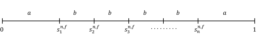
Figure 1: a canonical profile.

Lemma 3.5.

A game $G$ satisfying (HM1), (HM2), (HM3) has a canonical pair if and only if $\mathcal{H}^{\prime}(1/2)\leq\mathcal{M}^{\prime}(0)$. Moreover, if such a pair exists then it is unique.

Proof.

Let $\mathcal{H}^{\prime}(1/2)>\mathcal{M}^{\prime}(0)$, and assume towards contradiction that a canonical pair $\langle a,b\rangle$ exists. Note that $a\leq 1/2$ and $b\geq 0$ due to Eq. (9). Hence, since $\mathcal{H}^{\prime}$ and $\mathcal{M}^{\prime}$ are monotone decreasing, it follows that $\mathcal{H}^{\prime}(a)\geq\mathcal{H}^{\prime}(1/2)>\mathcal{M}^{\prime}(0)\geq\mathcal{M}^{\prime}(b)$, in contradiction to Eq. (8). This shows that no canonical pair exists if $\mathcal{H}^{\prime}(1/2)>\mathcal{M}^{\prime}(0)$.

Let $\mathcal{H}^{\prime}(1/2)\leq\mathcal{M}^{\prime}(0)$. We show that a canonical pair $\langle a,b\rangle$ exists. Note that for both (HM2) and (HM3) to hold we must have $\mathcal{H}^{\prime}(0)\geq\mathcal{M}^{\prime}(0)$, since otherwise $\mathcal{H}(\varepsilon)<\mathcal{M}(\varepsilon)$ for sufficiently small $\varepsilon>0$. Hence, by the monotonicity of $\mathcal{M}^{\prime}$,

$$\mathcal{H}^{\prime}(0)\geq\mathcal{M}^{\prime}(0)\geq\mathcal{M}^{\prime}\left(\frac{1}{n-1}\right)~{}.$$ (10)

Consider the function $g(x)=\mathcal{H}^{\prime}(x)-\mathcal{M}^{\prime}(\frac{1-2x}{n-1})$. By the assumption that $\mathcal{H}^{\prime}(1/2)\leq\mathcal{M}^{\prime}(0)$, we have that $g(1/2)\leq 0$, and by Eq. (10), it holds that $g(0)\geq 0$. Hence, by the intermediate value theorem there exists $x\in[0,1]$ such that $g(x)=0$. Thus, by definition, $\langle x,\frac{1-2x}{n-1}\rangle$ is a canonical pair. This shows that a canonical pair exists. It remains to show uniqueness.

Assume towards contradiction that $\langle a,b\rangle$ and $\langle a^{\prime},b^{\prime}\rangle$ are both canonical pairs, such that $a^{\prime}<a$. By Eq. (8),

$$\mathcal{H}^{\prime}(a)=\mathcal{M}^{\prime}(b)~{}~{}~{}~{}~{}~{}~{}\mbox{and}~{}~{}~{}~{}~{}~{}~{}\mathcal{H}^{\prime}(a^{\prime})=\mathcal{M}^{\prime}(b^{\prime})~{}.$$ (11)

Since $a^{\prime}<a$, by Eq. (9), it follows that $b^{\prime}>b$. $\mathcal{H}^{\prime}$ and $\mathcal{M}^{\prime}$ are strictly decreasing functions, so

$$\mathcal{H}^{\prime}(a)<\mathcal{H}^{\prime}(a^{\prime})~{}~{}~{}~{}~{}~{}~{}\mbox{and}~{}~{}~{}~{}~{}~{}~{}\mathcal{M}^{\prime}(b)>\mathcal{M}^{\prime}(b^{\prime})~{},$$

in contradiction to Eq. (11). Therefore $a^{\prime}=a$, which in turn ensures that also $b^{\prime}=b$. This shows that the canonical pair is unique, and concludes the proof of the claim. ∎

Theorem 3.6.

Let $G$ be a game satisfying (HM1),(HM2) and (HM3), and let $n=2$. The game $G$ has a unique Nash equilibrium, which is given by

$$\mathbf{s}^{*}=\left\{\begin{array}[]{ll}\;\;\mathbf{s}^{n,f}\;,&\mbox{if ~{}$\mathcal{H}^{\prime}(1/2)\leq\mathcal{M}^{\prime}(0)$;}\\ \left(\frac{1}{2},\frac{1}{2}\right),&\mbox{otherwise.}\end{array}\right.$$

Proof.

Let $(s_{1},s_{2})$ be a Nash equilibrium of the game. First note that $s_{1}\leq 1/2$, otherwise player 2 can improve its payoff by relocating to $1-s_{2}$ (due to the monotonicity $\mathcal{H}$ and $\mathcal{M}$). Symmetrically, we also have $s_{2}\geq 1/2$.

Consider the case where $\mathcal{H}^{\prime}(1/2)>\mathcal{M}^{\prime}(0)$, and suppose that $s_{2}>1/2$. We have that $s_{1}\leq 1/2$, so it follows from the monotonicity of $\mathcal{H}^{\prime}$ and $\mathcal{M}^{\prime}$ that $\mathcal{H}^{\prime}(s_{1})\geq\mathcal{H}^{\prime}(1/2)>\mathcal{M}^{\prime}(0)\geq\mathcal{M}^{\prime}(s_{2}-s)$. Therefore, by definition, $\theta_{s_{2}}(s_{1})>0$. It follows by Lemma 3.3 that $\rho(s_{2})$, the optimal location within the interval $[0,s_{2}]$, is not at $s_{1}$, contradiction. So suppose $s_{2}=1/2$ and thus $\mathcal{H}^{\prime}(s_{2})>\mathcal{M}^{\prime}(0)$. It follows, by Lemma 3.3, that the optimal location for player 1 is at $s_{1}=1/2$.

Now consider the case where $\mathcal{H}^{\prime}(1/2)\leq\mathcal{M}^{\prime}(0)$. It follows that $\mathcal{H}^{\prime}(s_{2})\leq\mathcal{M}^{\prime}(0)$ and $\mathcal{H}^{\prime}(1-s_{1})\leq\mathcal{M}^{\prime}(0)$, and thus by Lemma 3.3, we get

$$\mathcal{H}^{\prime}(s_{1})=\mathcal{M}^{\prime}(s_{2}-s_{1})\qquad\hbox{ and }\qquad\mathcal{H}^{\prime}(1-s_{2})=\mathcal{M}^{\prime}(s_{2}-s_{1})~{},$$

which yields $\mathcal{H}^{\prime}(s_{1})=\mathcal{H}^{\prime}(1-s_{2})$, and therefore $s_{1}=1-s_{2}$, due to the monotonicity of $\mathcal{H}^{\prime}$. It follows that $(x_{1},x_{2})$ is the canonical profile $\mathbf{s}^{n,f}$. We have shown that each player cannot improve locally, it remains to show each player cannot improve by moving to the other hinterland. Consider player 1 relocating to segment $[s_{2},1]$. By Claim 3.4(c), since $s_{2}>1/2$, we have that $\theta_{1-s_{2}}(\rho(1-s_{2}))\leq\theta_{s_{2}}(\rho(s_{2}))$, and thus the optimal location in $[s_{2},1]$ is not an improving move for player 1. This shows that player 1 has no improving move. Symmetrically, player 2 has no improving move, so this is a Nash equilibrium. Uniqueness follows from the uniqueness of the canonical pair (Lemma 3.5). ∎

For $n\geq 3$ players, we show that the only possible Nash equilibrium is the canonical profile. Towards proving Theorem 3.8, we state the following claim.

Lemma 3.7.

Let $G$ be a game satisfying (HM1),(HM2) and (HM3), and let $n\geq 3$. If $\mathbf{s}$ is a Nash equilibrium then no two players are colocated in $\mathbf{s}$.

Proof.

Assume towards contradiction that there exist players $i,i+1,\ldots,i+k$ such that $s_{i-1}<s_{i}=s_{i+1}=\cdots=s_{i+k}<s_{i+k+1}$ for $k\geq 1$. Suppose at first that these are internal players, i.e., $s_{1}<s_{i}<s_{n}$. Hence, by Lemma 3.2 the utility of $i$ is given by

$$u_{i}(\mathbf{s})=\frac{\mathcal{M}(s_{i}-s_{i-1})+\mathcal{M}(s_{i+k+1}-s_{i})}{k+1}~{}.$$

Assume without loss of generality that $\mathcal{M}(s_{i}-s_{i-1})\geq\mathcal{M}(s_{i+k+1}-s_{i})$. Note that

$$\max(\mathcal{M}(s_{i}-s_{i-1}),\mathcal{M}(s_{i+k+1}-s_{i}))\geq\frac{\mathcal{M}(s_{i}-s_{i-1})+\mathcal{M}(s_{i+k+1}-s_{i})}{2}~{}.$$

Therefore, if $k>1$ or $\mathcal{M}(s_{i}-s_{i-1})\neq\mathcal{M}(s_{i+k+1}-s_{i})$, then $s_{i}-\varepsilon$ is an improving move for player $i$, for sufficiently small $\varepsilon>0$. We may thus assume that $k=1$ and $\mathcal{M}(s_{i}-s_{i-1})=\mathcal{M}(s_{i+2}-s_{i})$ and thus $u_{i}(\mathbf{s})=\mathcal{M}(s_{i}-s_{i-1})$. But $\mathcal{M}$ is a concave function so $\mathcal{M}(s_{i}-s_{i-1})\leq 2\mathcal{M}((s_{i}-s_{i-1})/2)$. Therefore $(s_{i}+s_{i-1})/2$ is an improving move for player $i$, contradicting the assumption. We have shown that no Nash equilibrium $\mathbf{s}$ has colocated internal players. We next consider peripheral players.

Suppose now that $i=1$, that is, $s_{1}=s_{2}=\cdots=s_{k+1}<s_{k+2}$ for $k<n-1$ (i.e., not all players are colocated). Then by Lemma 3.2 the utility of player $k+1$ is given by

$$u_{k+1}(\mathbf{s})=\frac{\mathcal{H}(s_{k+1})+\mathcal{M}(s_{k+2}-s_{k+1})}{k+1}~{}.$$

As in the previous case, if $k>1$ or $\mathcal{H}(s_{k+1})\neq\mathcal{M}(s_{k+2}-s_{1})$, then player $1$ has an improving move. Hence, we assume $k=1$ and $\mathcal{H}(s_{2})=\mathcal{M}(s_{3}-s_{2})$. Therefore, $u_{2}(\mathbf{s})=\mathcal{M}(s_{3}-s_{2})$, and as above it follows from the concavity of $\mathcal{M}$ that $(s_{3}+s_{2})/2$ is a local improving move for player 2.

The only case left to consider is when all players are collocated at the same location, i.e., $s_{1}=s_{2}=\cdots=s_{n}$. Then by Lemma 3.2 the utility of player 1 is given by

$$u_{1}(\mathbf{s})=\frac{\mathcal{H}(s_{1})+\mathcal{H}(1-s_{1})}{n}~{}.$$

Since $n>2$, as in both previous cases player 1 can improve by moving to $s_{1}+\varepsilon$ for small enough $\varepsilon>0$. The claim follows.

∎

Theorem 3.8.

Let $G$ be a game satisfying (HM1),(HM2) and (HM3), and let $n\geq 3$. If the game $G$ admits a Nash equilibrium, then it is unique and equal to the canonical profile $\mathbf{s}^{n,f}$.

Proof.

By Lemma 3.7, no two players are colocated in $\mathbf{s}$. Our proof relies on local optimization of the location of each player. Assume towards contradiction that $\mathcal{H}^{\prime}(1/2)>\mathcal{M}^{\prime}(0)$. By Lemma 3.3, it follows that $u_{1}$, the utility of player 1, is an increasing function in the interval $[0,s_{2}]$ with respect to $s_{1}$, hence $(s_{1}+s_{2})/2$ is an improving move for player 1, in contradiction to $\mathbf{s}$ being an equilibrium. Thus, it must hold that $\mathcal{H}^{\prime}(1/2)\leq\mathcal{M}^{\prime}(0)$ .

Note that $s_{1}\leq 1/2$, otherwise player 2 can improve its payoff by relocating to $1-s_{2}$ (due to the monotonicity $\mathcal{H}$ and $\mathcal{M}$). Symmetrically, we also have $s_{2}\geq 1/2$. Thus, by Lemma 3.3, we have that

$$\mathcal{H}^{\prime}(s_{1})=\mathcal{M}^{\prime}(s_{2}-s_{1})~{}~{}~{}~{}~{}\mbox{and}~{}~{}~{}~{}~{}\mathcal{H}^{\prime}(1-s_{n})=\mathcal{M}^{\prime}(s_{n}-s_{n-1})~{}.$$ (12)

Additionally, by Lemma 3.3, we have that the optimal location of each internal player $i\in\{2,\dots,n-1\}$ is at $s_{i}=(s_{i-1}+s_{i+1})/2$. Consequently, there exists a constant $b$ such that $s_{2}-s_{1}=s_{3}-s_{2}=\cdots=s_{n}-s_{n-1}=b$. Pluggin $s_{2}-s_{1}=s_{n}-s_{n-1}$ into Eq. (12) we obtain

$$\mathcal{H}^{\prime}(s_{1})=\mathcal{H}^{\prime}(1-s_{n})~{},$$

and $\mathcal{H}^{\prime}$ is monotone decreasing since $\mathcal{H}$ is concave, so we get $s_{1}=1-s_{n}=a$, proving that $\mathbf{s}$ is a canonical profile. Uniqueness follows from Lemma 3.5. ∎

Lemma 3.9.

Let $G$ be a game satisfying (HM1),(HM2) and (HM3), and let $n\geq 3$. Let $\mathbf{s}^{n,f}$ be the canonical profile of $G$, with a corresponding canonical pair $\langle a,b\rangle$. Then $\mathbf{s}^{n,f}$ is a Nash equilibrium if and only if

$$\mathcal{H}(a)+\mathcal{M}(b) ~{}\geq~{}~{}2\mathcal{M}\left(\frac{b}{2}\right),$$ (13)

$$\mathcal{H}(\rho(a))+\mathcal{M}(a-\rho(a)) ~{}\leq~{}~{}2\mathcal{M}(b)~{}.$$ (14)

Proof.

By Lemma 3.3 we have that in each region there is one point that maximizes the payoff. Moreover, by Lemma 3.7 the payoff gained from colocating with another player $j$ can always be exceeded by that of an isolated location within one of $j$’s adjacent regions. Therefore, the canonical profile $\mathbf{s}^{n,f}$ is a Nash equilibrium if and only if relocating to the optimal location of any region is not an improving move for any player $i$.

Note that $\mathbf{s}^{n,f}$ is constructed such that no player $i$ can improve by moving to one of its adjacent regions, so it remains to consider whether $i$ can improve by moving to a non-adjacent region. It is easy to see that no internal player has an improving move in an internal region and that no peripheral player has an improving move in the other hinterland (due to the monotonicity of $\mathcal{H}$ and $\mathcal{M}$).

Let us consider the possibility that the peripheral player 1 has an improving move in an internal region. By Lemma 3.2, we have that $u_{1}(\mathbf{s}^{n,f})=\mathcal{H}(a)+\mathcal{M}(b)$, and by Lemma 3.3 the optimal utility player 1 would gain by relocating to an internal segment is $2\mathcal{M}(b/2)$. It follows that if Eq. (13) holds, then player 1 has no improving move.

We next consider whether an internal player $i\in\{2,\ldots,n-1\}$ has an improving move in the hinterland. By Lemma 3.2, we have that $u_{i}(\mathbf{s}^{n,f})=2\mathcal{M}(b)$, and by Lemma 3.3 the optimal utility player 1 would gain by relocating to a hinterland is $\mathcal{H}(\rho(a))+\mathcal{M}(a-\rho(a))$. It follows that if Eq. (14) holds, then player $i$ has no improving move. This shows that Eq. (13) and (14) are necessary and sufficient conditions for the canonical profile $\mathbf{s}^{n,f}$ to be a Nash equilibrium. ∎

4 Symmetric Range Distributions

In this section we consider the symmetric game $G^{S}(n,f)$, where the range of each client $v$ satisfies $B^{L}_{v}=B^{R}_{v}$. We first show that the game satisfies assumptions (HM1), (HM2) and (HM3), which allows us to use all the results of Section 3.

4.1 General Properties

Recall that $\bar{F}(t)=1-F(t)$, where $F$ is the cumulative distribution function of $f$.

Lemma 4.1.

Let $G^{S}(n,f)$ be a game such that $f$ is continuously differentiable and has full support (i.e., $f(x)>0$ for all $x\in[0,1]$), then $G^{S}(n,f)$ satisfies assumptions (HM1), (HM2) and (HM3).

Proof.

(HM2) and (HM3) follow immediately from Observation 3.1, so it remains to show (HM1). Note that by Observation 3.1, we have that $\mathcal{M}(x)=\mathcal{H}(x/2)$ for every $x\in[0,1]$, so it suffices to show that $\mathcal{H}$ is increasing and concave. By the fundamental theorem of calculus we obtain

$$\mathcal{H}^{\prime}(x)=1-F(x)~{},$$

which is strictly positive due to the fact that $f(x)>0$ for all $x\in[0,1)$ and thus not all of the mass of the distribution is contained in $[0,x]$. This shows that $\mathcal{H}$ is increasing.

We next show $\mathcal{H}$ is concave. By definition of $F$, the second derivative is

$$\mathcal{H}^{\prime\prime}(x)=-f(x)~{},$$

which is strictly negative by the assumption on $f$. It follows that $\mathcal{H}$ is concave. This proves the lemma. ∎

Due to Lemma 4.1, we may apply Theorem 3.6 and Theorem 3.8 to the game $G^{S}(n,f)$ and we thus obtain the following two corollaries.

Corollary 4.2.

Let $n=2$, and let $f$ be continuously differentiable and have full support (i.e., $f(x)>0$ for all $x\in[0,1]$). Then the game $G^{S}(2,f)$ has a unique Nash equilibrium, which is given by

$$\mathbf{s}^{*}=\left\{\begin{array}[]{ll}\;\;\mathbf{s}^{n,f}\;,&\mbox{if ~{}$\bar{F}(1/2)\leq 1/2$;}\\ \left(\frac{1}{2},\frac{1}{2}\right),&\mbox{otherwise,}\end{array}\right.$$

where $\mathbf{s}^{n,f}$ is the canonical profile, with a corresponding canonical pair $\langle a,b\rangle$, where $a$ and $b$ are given implicitly by the equation $\bar{F}(a)=\bar{F}(b/2)/2~{}.$

Corollary 4.3.

Let $n\geq 3$. For every game $G^{S}(n,f)$ where $f$ is continuously differentiable and has full support (i.e., $f(x)>0$ for all $x\in[0,1]$), if $G^{S}$ admits a Nash equilibrium then it is unique (up to renaming the players) and equal to the canonical profile $\mathbf{s}^{n,f}$, with a corresponding canonical pair $\langle a,b\rangle$, where $a$ and $b$ are given implicitly by the equation $\bar{F}(a)=\bar{F}(b/2)/2~{}.$

Lemma 4.4.

Under the symmetric game $G^{S}(n,f)$, the function $\rho:[0,1]\to[0,1]$ satisfies that $\rho(x)>x/3$, for all $x\in[0,1]$.

Proof.

Recall that $\rho(x)=\arg\max_{y\in[0,x]}\theta_{x}(y)$. Furthermore, by Lemma 3.3, $\theta_{x}$ is concave, so it follows that if $\theta^{\prime}_{x}(y)\geq 0$, (i.e., $\theta_{x}$ is non-decreasing at the point $y$) then $\rho(x)\geq y$. Thus, it suffices to show that $\theta_{x}(x/3)\geq 0$ for every $x\in[0,1]$. Plugging Eq. (3) and (4) into the definition of $\theta_{x}$ we obtain

$$\theta_{x}(y)=\int_{0}^{y}(1-F(t))dt+\int_{0}^{\frac{x-y}{2}}(1-F(t))dt~{}.$$

By the fundamental theorem of calculus, the derivative with respect to $y$ is given by

$$\theta^{\prime}_{x}(y)=1-F(y)-\frac{1}{2}\left(1-F\left(\frac{x-y}{2}\right)\right)~{}.$$

Plugging in $y=x/3$ yields

$$\theta^{\prime}_{x}\left(\frac{x}{3}\right)=1-F\left(\frac{x}{3}\right)-\frac{1}{2}\left(1-F\left(\frac{x}{3}\right)\right)=\frac{1}{2}\left(1-F\left(\frac{x}{3}\right)\right)\geq 0~{}.$$

This proves the claim. ∎

Lemma 4.5.

The game $G^{S}(n,f)$ as in Lemma 4.1, for $n\geq 3$, admits a Nash equilibrium if and only if

$$\mathcal{H}(\rho(a))+\mathcal{M}(a-\rho(a))\leq 2\mathcal{M}(b)~{},$$

where $\rho(a)$ is defined implicitly by the equation $\bar{F}(\rho(a))=\bar{F}((a-\rho(a))/2)/2$.

Proof.

By Lemma 4.1, $G^{S}(n,f)$ satisfies assumptions (HM1), (HM2) and (HM3). Therefore, by Lemma 3.9, $G^{S}(n,f)$ admits a Nash equilibrium if and only if Eq. (13) and (14) are satisfied. Recall that by the definition of the canonical profile, $a$ is the optimal location for player 1 within the interval $[0,a+b]$, i.e., $\rho(a+b)=a$. Thus, by Lemma 4.4, it follows that $a\geq(a+b)/3$, which yields $a\geq b/2$. by assumption (HM2) and the monotonicity of $\mathcal{H}$ and $\mathcal{M}$, we obtain

$$\mathcal{H}(a)+\mathcal{M}(b)\geq\mathcal{M}(a)+\mathcal{M}(b)\geq 2\mathcal{M}\left(\frac{b}{2}\right)$$

Thus, Eq. (13) always holds in the symmetric setting. Hence, the game admits a Nash equilibrium if and only if Eq. (14) is satisfied. The lemma follows. ∎

We conclude the discussion of symmetric games with a number of example distributions and their equilibria states.

4.2 Example 1: The Uniform Distribution

This distribution, in which the range boundary parameter $B^{L}_{v}$ ($=B^{R}_{v}$) is drawn uniformly at random from $[0,1]$, was considered by Ben-Porat and Tennenholtz [3] in a setting where clients are allowed to skip over players. Here we show that, if “skipping” is not allowed, as in our model, there is no Nash equilibrium for $n\geq 3$. For $n=2$, the only Nash equilibrium is $(1/2,1/2)$, where both players are colocated at the center. The probability density function and corresponding cumulative density function are defined as

$$f(x)=\left\{\begin{array}[]{l l}1,&x\in[0,1];\\ 0,&\mbox{otherwise,}\end{array}\right. F(x)=\left\{\begin{array}[]{l l}x,&x\in[0,1];\\ 1,&x\geq 1;\\ 0,&\mbox{otherwise.}\end{array}\right.$$          

Proposition 4.6.

For the game $G^{S}(n,f)$, where $f$ is the uniform distribution, there exists a Nash equilibrium if and only if $n=2$, and it is equal to the strategy profile $(1/2,1/2)$.

Proof.

Plugging $f$ into Corollary 4.3, we get that the only Nash equilibrium of $G^{S}(n,f)$ is the canonical profile represented by the canonical pair $\langle a,b\rangle$ where $a$ and $b$ satisfy $1-a=(1-b/2)/2$ By definition, the canonical pair additionally satisfies $2a+(n-1)b=1$. So the only solution is $a=1/2$ and $b=0$. Hence, $G^{S}(n,f)$ has a Nash equilibrium if and only if $n=2$. ∎

4.3 Example 2: Linear Distributions

Here we consider any distribution whose density is linear and whose mass is entirely contained in $[0,1]$. Specifically, assume $\int_{0}^{1}(rx+q)dx=1$, or rather $q=1-r/2$. For $f(x)$ to be non-negative in $[0,1]$ we also need $-2\leq r\leq 2$. Then take

$$f(x)=\left\{\begin{array}[]{l l}rx+q,&x\in[0,1];\\ 0,&\mbox{otherwise,}\end{array}\right. F(x)=\left\{\begin{array}[]{l l}\frac{r}{2}x^{2}+qx,&x\in[0,1];\\ 1,&x\geq 1;\\ 0,&\mbox{otherwise.}\end{array}\right.$$          

To make the analysis cleaner let us pick the two extreme examples of the parameters $(r,q)$, namely, $(-2,2)$ and $(2,0)$.

Proposition 4.7.

The game $G^{S}(n,f)$, where $f$ is the linear distribution with coefficients either $(r_{1},q_{1})=(-2,2)$ or $(r_{2},q_{2})=(2,0)$, has a Nash equilibrium if and only if $n=2$.

1. For $r_{1},q_{1}$, the only Nash equilibrium is (1/2,1/2).

2. For $r_{2},q_{2}$, the only (canonical) Nash equilibrium is given by the canonical pair

   $$a=\frac{2\sqrt{2}+1}{2\sqrt{2}+2}~{}~{}~{}~{}~{}~{}~{}~{}\mbox{and}~{}~{}~{}~{}~{}~{}~{}~{}b=\frac{\sqrt{2}-1}{1+1/\sqrt{2}}~{}.$$

Proof.

For $r_{2},q_{2}$ we get that $\bar{F}(1/2)>1/2$ and thus by Corollaries 4.2 and 4.3 the only Nash equilibrium is $(1/2,1/2)$ when $n=2$.

For $r_{1},q_{1}$ we get the equation $(1-a)^{2}=\frac{1}{2}(1-b/2)^{2}$, which yields

$$a=\frac{2(\sqrt{2}-1)n-2\sqrt{2}+3}{2\sqrt{2}(n-1)+2}~{}~{}~{}~{}~{}~{}~{}~{}\mbox{and}~{}~{}~{}~{}~{}~{}~{}~{}b=\frac{\sqrt{2}-1}{n-1+1/\sqrt{2}}~{}.$$

If $n=2$, a Nash equilibrium always exists, so this is a Nash equilibrium. For $n\geq 3$, by Lemma 4.5 this is a Nash equilibrium if for every $x$ in $[0,a]$ we have

$$\left(1-\frac{a-x}{2}\right)^{3}+(1-x)^{3}\geq 2\left(1-\frac{b}{2}\right)^{3}~{}.$$ (15)

But $a\geq 2b$ so we can choose $x$ such that $x\geq b/2$ and $(a-x)/2\geq b/2$, making the left hand side of Ineq. (15) strictly smaller than the right hand side, contradiction. Hence there is no Nash equilibrium. ∎

Remark. Intuitively, in the uniform distribution the players are forced to converge towards the center. In comparison, in the linear distribution corresponding to $(r_{2},q_{2})$ it is likelier for clients to have a large range, which means more clients inside the hinterland will be covered by the peripheral player, so it will be beneficial for it to move closer to its neighbor and have fewer clients contested by another player, despite having a greater average distance to potential clients.

4.4 Example 3: Pareto Distributions

The distribution $\mbox{Pareto}(\alpha,\xi)$ for parameters $\alpha>0$ and $\xi>0$ has density function and cumulative distribution function

$$f(x)=\left\{\begin{array}[]{l l}0,&x<\xi~{};\\ \frac{\alpha\xi^{\alpha}}{x^{\alpha+1}},&x\geq\xi~{},\end{array}\right. F(x)=\left\{\begin{array}[]{l l}0,&x<\xi~{};\\ 1-\left(\xi/x\right)^{\alpha},&x\geq\xi~{}.\end{array}\right.$$          

Proposition 4.8.

For the game $G^{S}(n,f)$, where $f$ is the density of $\mbox{Pareto}(\alpha,\xi)$, the canonical pair is given by

$$a=\frac{2^{1/\alpha-1}}{n-1+2^{1/\alpha}}~{}~{}~{}~{}~{}~{}~{}~{}\mbox{and}~{}~{}~{}~{}~{}~{}~{}~{}b=\frac{1}{n-1+2^{1/\alpha}}~{},$$ (16)

and it is a Nash equilibrium if and only if $\alpha\geq z$, where $z$ is the unique solution of the equation $2^{1/z}(2+2^{1/z})^{z}=8$ such that $0<z<1$.

Proof.

Note that $f(x)=0$ for $x\in[0,\xi)$ so the conditions of Corollary 4.3 do not apply. However, for $\xi$ small enough the result still holds. The equation $\bar{F}(a)=\bar{F}(b/2)/2$ yields

$$\left(\frac{\xi}{a}\right)^{\alpha}=\frac{1}{2}\left(\frac{2\xi}{b}\right)^{\alpha}~{},$$

which translates to $a=2^{1/\alpha-1}b$. By definition the canonical pair satisfies $2a+(n-1)b=1$. So we get

$$a=\frac{2^{1/\alpha-1}}{n-1+2^{1/\alpha}}~{}~{}~{}~{}~{}~{}~{}~{}\mbox{and}~{}~{}~{}~{}~{}~{}~{}~{}b=\frac{1}{n-1+2^{1/\alpha}}~{}.$$ (17)

To apply Lemma 4.5 we first calculate

$$\int_{0}^{x}\bar{F}(t)dt=\left\{\begin{array}[]{l l}\xi+\xi\ln\left(\frac{x}{\xi}\right),&\alpha=1~{};\\ \xi+\frac{\xi}{\alpha-1}\left(1-\left(\frac{\xi}{x}\right)^{\alpha-1}\right),&\alpha\neq 1~{}.\end{array}\right.$$

Let $x^{*}\in[0,a]$ satisfy

$$\bar{F}(x^{*})=\bar{F}((a-x^{*})/2)/2.$$

This solves to

$$x^{*}=\frac{2^{1/\alpha}a}{2+2^{1/\alpha}}~{}~{}~{}~{}~{}~{}~{}~{}\mbox{and}~{}~{}~{}~{}~{}~{}~{}~{}\frac{a-x^{*}}{2}=\frac{a}{2+2^{1/\alpha}}$$ (18)

Consider $\alpha=1$ first. Note that in this case, $a=b$ and $x^{*}=a/2$, so the condition given in Lemma 4.5 translates to

$$\int_{\frac{a}{4}}^{\frac{a}{2}}\bar{F}(t)dt\geq\int_{\frac{a}{2}}^{\frac{a}{2}}\bar{F}(t)dt~{}.$$

This always holds since the left hand side is non-negative and the right hand side is zero. So we have that for $\alpha=1$ the canonical pair is $\langle\frac{1}{n+1},\frac{1}{n+1}\rangle$ and it is a Nash equilibrium.

Let us now consider $\alpha\neq 1$. By Lemma 4.5 the canonical profile given in (17) is a Nash equilibrium if and only if

$$\frac{\xi}{\alpha-1}\left(\left(\frac{2\xi}{a-x^{*}}\right)^{\alpha-1}-\left(\frac{2\xi}{b}\right)^{\alpha-1}\right)\geq\frac{\xi}{\alpha-1}\left(\left(\frac{2\xi}{b}\right)^{\alpha-1}-\left(\frac{\xi}{x^{*}}\right)^{\alpha-1}\right)~{}.$$

Rearranging, we obtain

$$\frac{1}{\alpha-1}\left(\left(\frac{2}{a-x^{*}}\right)^{\alpha-1}+\left(\frac{1}{x^{*}}\right)^{\alpha-1}\right)\geq\frac{2}{\alpha-1}\left(\frac{2}{b}\right)^{\alpha-1}~{}.$$

Plugging $b=2^{1-1/\alpha}a$ and Eq. (18) in the above we get

$$\frac{1}{\alpha-1}\left(\left(\frac{2+2^{1/\alpha}}{a}\right)^{\alpha-1}+\left(\frac{2+2^{1/\alpha}}{2^{1/\alpha}a}\right)^{\alpha-1}\right)\geq\frac{2}{\alpha-1}\left(\frac{2^{1/\alpha}}{a}\right)^{\alpha-1}~{}.$$

Suppose $\alpha>1$. We get

$$(2+2^{1/\alpha})^{\alpha-1}\left(\frac{1}{2^{(\alpha-1)/\alpha}}+1\right)\geq 8\cdot 2^{-1/\alpha}$$

or $2^{1/\alpha}(2+2^{1/\alpha})^{\alpha}\geq 8$. This inequality holds since equality holds for $\alpha=1$ and the left hand side is a monotonically increasing function of $\alpha$ for $\alpha>1$.

Now consider $\alpha<1$. We get $2^{1/\alpha}(2+2^{1/\alpha})^{\alpha}\leq 8~{}.$ There exists a constant $0<z<1$ such that $2^{1/z}(2+2^{1/z})^{z}=8$. The inequality holds for $\alpha\in[z,1]$.

To summarize, we have that for $\alpha\geq z$ the game has a unique Nash equilibrium which is the canonical profile given in Eq. (17). ∎

4.5 Example 4: Exponential Distributions

The exponential distribution with parameter $\lambda>0$ has density function and cumulative density function

$$f(x)=\left\{\begin{array}[]{l l}0,&x<0~{};\\ \lambda e^{-\lambda x},&x\geq 0~{},\end{array}\right. F(x)=\left\{\begin{array}[]{l l}0,&x<0~{};\\ 1-e^{-\lambda x},&x\geq 0~{}.\end{array}\right.$$          

Proposition 4.9.

For the game $G^{S}(n,f)$, where $f$ is the density of the exponential distribution with parameter $\lambda>0$, the canonical pair is given by

$$a=\frac{1}{n}\left(\frac{1}{2}+\frac{(n-1)\ln 2}{\lambda}\right)~{}~{}~{}~{}~{}~{}~{}~{}\mbox{and}~{}~{}~{}~{}~{}~{}~{}~{}b=\frac{1}{n}\left(1-\frac{2\ln 2}{\lambda}\right)$$

and it is a Nash equilibrium if and only if $\lambda\geq\ln 4-n\ln(4\tau_{1}^{6})$, where $\tau_{1}=\frac{\sqrt[6]{2}+\sqrt{64+\sqrt[3]{2}}}{8\cdot 2^{5/6}}\approx 0.65$.

Proof.

By Corollary 4.3 we have that the only Nash equilibrium of the game $G^{S}(n,f)$ is the canonical pair $\langle a,b\rangle$ satisfying

$$e^{-\lambda a}=e^{-\lambda b/2}/2~{},$$

and thus $a=b/2+\ln 2/\lambda$. By definition, $a$ and $b$ satisfy $2a+(n-1)b=1$ and therefore we obtain

$$a=\frac{1}{n}\left(\frac{1}{2}+\frac{(n-1)\ln 2}{\lambda}\right)~{}~{}~{}~{}~{}~{}~{}~{}\mbox{and}~{}~{}~{}~{}~{}~{}~{}~{}b=\frac{1}{n}\left(1-\frac{2\ln 2}{\lambda}\right)$$

By Lemma 4.5 the canonical profile is a Nash equilibrium if and only if

$$\int_{\frac{a-x^{*}}{2}}^{\frac{b}{2}}e^{-\lambda t}dt\geq\int_{\frac{b}{2}}^{x^{*}}e^{-\lambda t}dt$$ (19)

where $x^{*}\in[0,a]$ is the unique solution of

$$e^{-\lambda x^{*}}=e^{-\lambda(a-x^{*})/2}/2~{}.$$

So we get

$$x^{*}=\frac{a}{3}+\frac{2\ln 2}{3\lambda}~{}~{}~{}~{}~{}~{}~{}~{}\mbox{and}~{}~{}~{}~{}~{}~{}~{}~{}\frac{a-x^{*}}{2}=\frac{a}{3}-\frac{\ln 2}{3\lambda}~{}.$$

Plugging the above along with $b/2=a-\ln 2~{}/\lambda$ into Eq. (19) we get

$$\sqrt[3]{2}e^{-\lambda a/3}+e^{-2\lambda a/3}/{\sqrt[3]{4}}\geq 4e^{-\lambda a}~{}.$$

Let $\tau=e^{-\lambda a/3}$. The above inequality translates into

$$4\tau^{3}-\tau^{2}/{\sqrt[3]{4}}-\sqrt[3]{2}\tau\leq 0~{}.$$

Solving the inequality we get $0\leq\tau\leq\tau_{1}$, where $\tau_{1}=\frac{\sqrt[6]{2}+\sqrt{64+\sqrt[3]{2}}}{8\cdot 2^{5/6}}\approx 0.65$. Plugging $\tau=e^{-\lambda a/3}$ back in we obtain

$$\lambda a\geq-3\ln\tau_{1}~{},$$

and plugging in $a=\frac{1}{n}\left(\frac{1}{2}+\frac{(n-1)\ln 2}{\lambda}\right)$ we obtain

$$\lambda\geq\ln 4-n\ln(4\tau_{1}^{6})\approx 1.39+1.24n$$

as the necessary and sufficient condition for the existence of a Nash equilibrium under the exponential distribution. ∎

5 Asymmetric Range Distributions

In this section we consider the asymmetric game $G^{A}(n,f)$, where the range boundaries of each client $v$, $B^{L}_{v}$ and $B^{R}_{v}$, are drawn independently at random. As in the previous section, we begin by showing that the game satisfies assumptions (HM1), (HM2) and (HM3), allowing us to use the results of Section 3.

5.1 General Properties

Lemma 5.1.

Let $G^{A}(n,f)$ be a game such that $f$ is continuously differentiable and has full support (i.e., $f(x)>0$ for all $x\in[0,1]$), then $G^{A}(n,f)$ satisfies assumptions (HM1), (HM2) and (HM3).

Proof.

(HM2) and (HM3) follow immediately from Observation 3.1, so it remains to show (HM1). Note that by Observation 3.1, $\mathcal{H}$ is the same as in the symmetric game $G^{S}(n,f)$, and thus by Lemma 4.1, $\mathcal{H}$ is increasing and concave. It remains to show that $\mathcal{M}$ is monotone and concave. Using the Leibniz integral differentiation rule we obtain

$$\mathcal{M}^{\prime}(x)=\frac{1}{2}\left(1-F\left(\frac{x}{2}\right)\right)^{2}+\int_{\frac{x}{2}}^{x}(1-F(t))f(x-t)dt>0~{}.$$

Hence, $\mathcal{M}$ is monotone increasing. Taking the second derivative with respect to $x$ yields

$$\mathcal{M}^{\prime\prime}(x)=-\left(1-F\left(\frac{x}{2}\right)\right)f\left(\frac{x}{2}\right)+(1-F(x))f(0)+\int_{\frac{x}{2}}^{x}(1-F(t))f^{\prime}(x-t)dt$$

and using integration by parts we get

$$\mathcal{M}^{\prime\prime}(x)=-\left(1-F\left(\frac{x}{2}\right)\right)f\left(\frac{x}{2}\right)+(1-F(x))f(0)+(1-F(t))f(x)|_{\frac{x}{2}}^{x}-\int_{\frac{x}{2}}^{x}f(t)(f(x-t))dt$$

$$=-\int_{\frac{x}{2}}^{x}f(t)f(x-t)dt<0$$

Hence, the function $\mathcal{M}$ is concave, and thus the lemma holds. ∎

Due to Lemma 5.1, we may apply Theorem 3.6 and Theorem 3.8 to the game $G^{A}(n,f)$ and we thus obtain the following two corollaries.

Corollary 5.2.

Let $n=2$, and let $f$ be continuously differentiable and have full support (i.e., $f(x)>0$ for all $x\in[0,1]$). Then the game $G^{A}(2,f)$ has a unique Nash equilibrium, which is given by

$$\mathbf{s}^{*}=\left\{\begin{array}[]{ll}\;\;\mathbf{s}^{n,f}\;,&\mbox{if ~{}$\bar{F}(1/2)\geq 1/2$;}\\ \left(\frac{1}{2},\frac{1}{2}\right),&\mbox{otherwise,}\end{array}\right.$$

where $\mathbf{s}^{n,f}$ is the canonical profile, with a corresponding canonical pair $\langle a,b\rangle$, where $a$ and $b$ are given implicitly by the equation

$$\bar{F}(a)=\frac{1}{2}\left(\bar{F}\left(\frac{b}{2}\right)\right)^{2}+\int_{\frac{b}{2}}^{b}\bar{F}(t)f(b-t)dt$$

Corollary 5.3.

Let $n\geq 3$. For every game $G^{A}(n,f)$ where $f$ has full support (i.e., $f(x)>0$ for all $x\in[0,1]$), if $G^{A}$ admits a Nash equilibrium it is unique (up to renaming the players) and equal to the canonical profile $\langle a,b\rangle$ where $a$ and $b$ are given implicitly by the equation

$$\bar{F}(a)~{}=~{}\frac{1}{2}\left(\bar{F}\left(\frac{b}{2}\right)\right)^{2}+\int_{\frac{b}{2}}^{b}\bar{F}(t)f(b-t)dt~{}.$$

Lemma 5.4.

Under the asymmetric game $G^{A}(n,f)$, the function $\rho:[0,1]\to[0,1]$ satisfies that $\rho(x)>x/3$, for all $x\in[0,1]$.

Proof.

Recall that $\rho(x)=\arg\max_{y\in[0,x]}\theta_{x}(y)$. Furthermore, by Lemma 3.3, $\theta_{x}$ is concave, so it follows that if $\theta^{\prime}_{x}(y)\geq 0$, (i.e., $\theta_{x}$ is non-decreasing at the point $y$) then $\rho(x)\geq y$. Thus, it suffices to show that $\theta_{x}(x/3)\geq 0$ for every $x\in[0,1]$. Plugging Eq. (5) and (6) into the definition of $\theta_{x}$ we obtain

$$\theta_{x}(y)=\int_{0}^{y}(1-F(t))dt+\int_{0}^{\frac{x-y}{2}}(1-F(t))dt+\int_{\frac{x-y}{2}}^{x-y}(1-F(t))F(x-y-t)dt~{}.$$

By Leibniz’s integral rule, the derivative with respect to $y$ is given by

$$\theta^{\prime}_{x}(y)=1-F(y)-\frac{1}{2}\left(1-F\left(\frac{x-y}{2}\right)\right)^{2}-\int_{\frac{x-y}{2}}^{x-y}(1-F(t))f(x-y-t)dt~{}.$$

Plugging in $y=x/3$ yields

$$\theta^{\prime}_{x}\left(\frac{x}{3}\right)=1-F\left(\frac{x}{3}\right)-\frac{1}{2}\left(1-F\left(\frac{x}{3}\right)\right)^{2}-\int_{\frac{x}{3}}^{\frac{2x}{3}}(1-F(t))f\left(\frac{2x}{3}-t\right)dt~{},$$

using differentiation by parts and rearranging we obtain

$$\theta^{\prime}_{x}\left(\frac{x}{3}\right)=\frac{1}{2}\left(1-F\left(\frac{x}{3}\right)\right)^{2}+\int_{\frac{x}{3}}^{\frac{2x}{3}}f(t)f\left(\frac{2x}{3}-t\right)dt\geq 0~{},$$

which proves the claim. ∎

Lemma 5.5.

The game $G^{A}(n,f)$ admits a Nash equilibrium if and only if

$$\mathcal{H}(\rho(a))+\mathcal{M}(a-\rho(a))\leq 2\mathcal{M}(b)~{},$$ (20)

where $\rho(x)$ is defined implicitly by the equation

$$\bar{F}(\rho(x))=\frac{1}{2}\left(\bar{F}\left(\frac{a-\rho(x)}{2}\right)\right)^{2}+\int_{\frac{a-\rho(x)}{2}}^{a-\rho(x)}\bar{F}(t)f(a-\rho(x)-t)dt~{}.$$

Proof.

By Lemma 5.1, $G^{A}(n,f)$ satisfies assumptions (HM1), (HM2) and (HM3). Therefore, by Lemma 3.9, $G^{A}(n,f)$ admits a Nash equilibrium if and only if Eq. (13) and (14) are satisfied. Recall that by the definition of the canonical profile, $a$ is the optimal location for player 1 within the interval $[0,a+b]$, i.e., $\rho(a+b)=a$. Thus, by Lemma 5.4, it follows that $a\geq(a+b)/3$, which yields $a\geq b/2$. Therefore, by assumption (HM2) and the monotonicity of $\mathcal{H}$ and $\mathcal{M}$, we obtain

$$\mathcal{H}(a)+\mathcal{M}(b)\geq\mathcal{M}(a)+\mathcal{M}(b)\geq 2\mathcal{M}\left(\frac{b}{2}\right)$$

Thus, Eq. (13) always holds in the asymmetric setting. Hence, the game admits a Nash equilibrium if and only if Eq. (14) is satisfied. The lemma thus follows. ∎

Theorem 5.6.

If $G^{S}(n,f)$ admits a Nash equilibrium and

$$\frac{\partial}{\partial x}\left(\int_{\frac{x}{2}}^{x}\bar{F}(t)F(b-t)dt\right)\geq 0,$$

then $G^{A}(n,f)$ admits a Nash equilibrium.

Proof.

If $n=2$, by Theorem 3.6, the theorem holds. Assume $n\geq 3$. To simplify notation, let $\mathbf{s}=\mathbf{s}^{n,f}$, be the canonical profile of $G^{S}(n,f)$. Let $\langle a,b\rangle$ the canonical pair of $G^{S}(n,f)$. Let $\widetilde{u}_{i}$ denote the utility of player $i$ in the game $G^{A}(n,f)$. Similarly, throughout this proof, we use the notation $\widetilde{\mathcal{H}}$, $\widetilde{\mathcal{M}}$ and $\widetilde{\rho}$ when referring to $G^{A}(n,f)$, while the original notation refers to $G^{S}(n,f)$. Let

$$\Delta(x)=\int_{\frac{x}{2}}^{x}\bar{F}(t)F(b-t)dt~{}.$$

Note that by Observation 3.1 we have that $\widetilde{\mathcal{M}}(x)=\mathcal{M}(x)+\Delta(x)$ and $\widetilde{\mathcal{H}}(x)=\mathcal{H}(x)$ for every $x\in[0,1]$, and therefore for every internal player $i\in\{2,\ldots,n-1\}$ we have that

$$u_{i}(\mathbf{s})=\widetilde{u}_{i}(\mathbf{s})+2\Delta(b)$$

and for peripheral players

$$u_{1}(\mathbf{s})=\widetilde{u}_{1}(\mathbf{s})+\Delta(b)~{}~{}~{}~{}~{}\mbox{and}~{}~{}~{}~{}u_{n}(\mathbf{s})=\widetilde{u}_{n}(\mathbf{s})+\Delta(b)~{}.$$

Let $x^{*}=\rho(a)$ denote the best response in the hinterland $(0,a)$ in the game $G^{S}(n,f)$, and let $\widetilde{x}^{*}=\widetilde{\rho}(a)$ denote the best response in the hinterland $(0,a)$ in the game $G^{A}(n,f)$. Since $\mathbf{s}$ is a Nash equilibrium in $G^{S}(n,f)$ we have that

$$u_{i}(\mathbf{s})\geq u_{i}(x^{*},\mathbf{s}_{-i}),$$

which can be written as

$$2\mathcal{M}(b)\geq\mathcal{H}(x^{*})+\mathcal{M}(a-x^{*})$$ (21)

Assume towards contradiction that $a-\widetilde{x}^{*}>b$. Due to Lemma 5.4 we get $b\leq 2\widetilde{x}^{*}$, and it thus by monotonicity of $\mathcal{M}$ and since $\mathcal{M}(x)=\mathcal{H}(x/2)$ we get

$$u_{i}(\mathbf{s})=2\mathcal{M}(b)<\mathcal{M}(2\widetilde{x}^{*})+\mathcal{M}(a-\widetilde{x}^{*})=\mathcal{H}(\widetilde{x}^{*})+\mathcal{M}(a-\widetilde{x}^{*})=u_{i}(\widetilde{x}^{*},\mathbf{s}_{-i})~{},$$

in contradiction to $\mathbf{s}$ being a Nash equilibrium in the symmetric game $G^{S}(n,f)$. Hence, $a-\widetilde{x}^{*}\leq b$. Moreover, by assumption, $\Delta(x)$ is increasing with respect to $x$, so we have that

$$\Delta(a-\widetilde{x}^{*})\leq\Delta(b)$$

Therefore,

$$\widetilde{u}_{i}(\widetilde{x}^{*},\mathbf{s}_{-i})=\widetilde{\mathcal{H}}(\widetilde{x}^{*})+\widetilde{\mathcal{M}}(a-\widetilde{x}^{*}) =\mathcal{H}(\widetilde{x}^{*})+\mathcal{M}(a-\widetilde{x}^{*})+\Delta(a-\widetilde{x}^{*})$$

$$\leq\mathcal{H}(x^{*})+\mathcal{M}(a-x^{*})+\Delta(a-\widetilde{x}^{*})~{},$$

where the last inequality is due to the optimality of $x^{*}$ with respect to the function $\mathcal{H}(t)+\mathcal{M}(a-t)$. But $\Delta(a-\widetilde{x}^{*})\leq\Delta(b)$, so plugging Equation (21) in the above we get

$$\widetilde{\mathcal{H}}(\widetilde{x}^{*})+\widetilde{\mathcal{M}}(a-\widetilde{x}^{*})\leq 2\mathcal{M}(b)+\Delta(b)\leq 2\widetilde{\mathcal{M}}(b)=\widetilde{u}_{i}(\mathbf{s})$$ (22)

Therefore, there is no improving move for an internal player in $G^{A}(n,f)$ under $\mathbf{s}$.

Let $\langle\widetilde{a},\widetilde{b}\rangle$ be the canonical pair of $G^{A}(n,f)$, and let $\widetilde{\mathbf{s}}=\widetilde{\mathbf{s}}^{n,f}$ be the corresponding canonical profile. If we show that $\widetilde{b}\geq b$, then Equation (20) would hold, which would conclude the proof by Lemma 5.5. This is due to the fact that

$$2\widetilde{\mathcal{M}}(\widetilde{b})\geq 2\widetilde{\mathcal{M}}(b)\geq\widetilde{\mathcal{H}}(\widetilde{x}^{*})+\widetilde{\mathcal{M}}(a-\widetilde{x}^{*})\geq\widetilde{\mathcal{H}}(\widetilde{\rho}(\widetilde{a}))+\widetilde{\mathcal{M}}(\widetilde{a}-\widetilde{\rho}(\widetilde{a}))~{},$$

where the first inequality is due to the monotonicity of $\widetilde{\mathcal{M}}$, the second inequality is due to Equation (22), and the last inequality is due to Lemma 3.4(c). Hence, it remains to show that $\widetilde{b}\geq b$.

We will show that $\widetilde{a}\leq a$, which is equivalent. Consider the function $g(x)=\widetilde{\mathcal{H}}^{\prime}(x)-\widetilde{\mathcal{M}}^{\prime}((1-2x)/(n-1))$. By the definition of the canonical pair, we have that $g(\widetilde{a})=0$. Moreover, by concavity of $\widetilde{\mathcal{H}}$ and $\widetilde{\mathcal{M}}$ we have that $g$ is decreasing, and by Lemma 3.5 it has at most one zero. Hence, every $x$ such that $g(x)\leq 0$ must satisfy $x\geq\widetilde{a}$. Furthermore,

$$g(a)=\widetilde{\mathcal{H}}^{\prime}(a)-\widetilde{\mathcal{M}}^{\prime}((1-2a)/(n-1))=\mathcal{H}^{\prime}(a)-\mathcal{M}^{\prime}(b)-\Delta^{\prime}(b)=-\Delta^{\prime}(b)\leq 0~{},$$

where the second and third equalities are due to $\langle a,b\rangle$ being a canonical pair, and the last inequality is due to the assumption. Thus, $\widetilde{a}\leq a$, which concludes the proof. ∎

Again we conclude with a couple of example distributions and their equilibria.

5.2 Example 1: The Uniform Distribution

This is the same as the uniform distribution for symmetric games, except that both range boundary parameters $B^{L}_{v}$ and $B^{L}_{v}$ need to be drawn uniformly at random. We have the following.

Proposition 5.7.

For the game $G^{A}(n,f)$, where $f$ is the uniform distribution, there exists a Nash equilibrium if and only if $n=2$, and it is equal to the strategy profile $(1/2,1/2)$.

Proof.

Using Corollary 5.3, we get

$$1-a=\frac{1}{2}\left(1-\frac{b}{2}\right)^{2}+\int_{\frac{b}{2}}^{b}(1-t)dt~{},$$

which translates to

$$1-a=1/2-b^{2}/4~{}.$$

By definition $\langle a,b\rangle$ satisfies $2a+(n-1)b=1$. So, as in the symmetric setting, we get that the only solution is $a=\frac{1}{2}$ and $b=0$. Hence, $G^{A}(n,f)$ has a Nash equilibrium if and only if $n=2$. ∎

5.3 Example 2: The Exponential Distribution

Finally, we consider the game $G^{A}(n,f)$ where $f$ is the density function of the exponential distribution with parameter $\lambda>0$. That is, the range of each client $v$ is asymmetric and exponentially distributed, i.e., $B^{L}_{v},B^{R}_{v}\in\mbox{Exp}(\lambda)$. Slightly abusing notation, we refer to this game as $G^{A}(n,\lambda)$. We dedicate special attention to this distribution for three main reasons. First, the exponential distribution is commonly considered in geometric models, and has been shown to apply to many real life situations. Second, the game $G^{A}(n,\lambda)$ is mathematically equivalent to a fault-prone Hotelling game, studied in our related paper [7]. In this game, faults occur at random along the line, and clients cannot visit players separated from them by a random fault. Hence, our results on the exponential distribution can be applied directly to fully characterize the equilibria of another interesting variant of the Hotelling model. Finally, this example demonstrates that even though the condition of Theorem 5.6 does not always apply to the exponential distribution, and the condition given for the existence of Nash equilibria in Lemma 5.5 is somewhat hard to work with, it is nevertheless possible to fully analyze certain useful classes of client range distributions.

By Corollary 5.2, if $n=2$ then the game always admits a Nash equilibrium, which is the canonical profile if it exists, and $(1/2,1/2)$ otherwise. For $n\geq 3$, by Corollary 5.3, if the game admits a Nash equilibrium then it is equal to the canonical profile. Consequently, to fully characterize the equilibria of the game, the following theorem determines, for any given $n$ and $\lambda$, whether the canonical pair of $G^{A}(n,\lambda)$ is Nash equilibrium. More precisely, the theorem characterizes a threshold function $\lambda_{\min}(n)$ such that the game $G^{A}(n,\lambda)$ admits a Nash equilibrium if and only if $\lambda\geq\lambda_{\min}(n)$.

Moreover, the exact formulation of the threshold function $\lambda_{\min}(n)$ depends on a global constant $\alpha_{0}$. While there is no closed form formula for $\alpha_{0}$, it is implicitly defined as the unique solution of Eq. (23) and (24) in the interval $[0,1]$ (see Figure 2), which is approximately $\alpha_{0}\approx 0.58813$.

Theorem 5.8.

$G^{A}(n,\lambda)$ for $n\geq 3$ admits a Nash equilibrium if and only if

$$\lambda~{}\geq~{}\lambda_{\min}(n)~{}=~{}(n+1)\alpha_{0}-2\ln\left(\frac{1+\alpha_{0}}{2}\right)~{},$$

where $\alpha_{0}\in(0,1)$ is the unique constant given implicitly as the solution to the following equations:

$$e^{-\alpha}(1+\alpha) =e^{-2\beta}(1+\beta)~{},$$ (23)

$$e^{-\alpha}\left(1+\frac{\alpha}{2}\right) =e^{-\beta}\left(\frac{3}{4}+\frac{\beta}{2}\right)~{}.$$ (24)

Moreover, $\alpha_{0}\approx 0.58813$, implying that a Nash equilibrium exists if and only if

$$\lambda~{}\geq~{}\lambda_{\min}(n)~{}\approx~{}0.58813n+1.04931~{}.$$

We start our analysis by deriving the functions $\mathcal{H}$ and $\mathcal{M}$ by plugging the cumulative distribution function of $\mbox{Exp}(\lambda)$, i.e., $F(t)=1-e^{-\lambda t}$ into Eq. (5) and (6). This yields

$$\mathcal{H}(x)= \frac{1}{\lambda}\left[1-e^{-\lambda x}\right]$$ (25)

$$\mathcal{M}(x)= \frac{1}{\lambda}\left[1-e^{-\lambda x}\left(1+\frac{\lambda x}{2}\right)\right]$$ (26)

We can characterize the canonical pair of the game $G^{A}(n,\lambda)$, provided it exists. By Corollary 5.3, given an integer $n\geq 2$ and a real $\lambda>0$, the canonical pair $\langle a,b\rangle$ exists if and only if $\lambda>2\ln 2$ and is given by the following equations:

$$e^{\lambda(b-a)}=\frac{1+\lambda b}{2}$$ (27)

$$2a+(n-1)b=1$$ (28)

By Lemma 5.5, in order to prove Theorem 5.8, it suffices to show that making a non-local move, namely, relocating an internal player to $\rho(a)$, the optimal location within the hinterland, is not improving. Plugging Eq. (25) and (26) into the definition of $\rho(x)$, we obtain that in the game $G^{A}(n,\lambda)$, for every $x\in[\ln 2/\lambda,1]$, $\rho(x)$ is given implicitly by

$$e^{\lambda(x-2\rho(x))}=\frac{1+\lambda(x-\rho(x))}{2}$$ (29)

Lemma 5.9.

Let $x\in[\ln 2/\lambda,1]$. Then,

$$\mathcal{H}(\rho(x))=\mathcal{M}(x-\rho(x))+\frac{1}{2\lambda}e^{-\lambda(x-\rho(x))}$$

Proof.

By Eq. (25),

$$\mathcal{H}(\rho(x))=\frac{1}{\lambda}\left[1-e^{-\lambda\rho(x)}\right]$$

Plugging in Eq. (29), we get

$$\mathcal{H}(\rho(x)) =\frac{1}{\lambda}\left[1-e^{-\lambda(x-\rho(x))}\left(\frac{1+\lambda(x-\rho(x))}{2}\right)\right]$$

$$=\frac{1}{\lambda}\left[1-e^{-\lambda(s-\rho(x))}\left(1+\frac{\lambda(x-\rho(x))}{2}\right)\right]+\frac{1}{2\lambda}e^{-\lambda(x-\rho(x))}$$

Plugging in Eq. (26) we obtain the result. ∎

Before we continue, we define a reparamatrization that will greatly simplify the following analysis. Define

$$\alpha=\lambda b~{}~{}~{}~{}\mbox{and}~{}~{}~{}~{}c=1-a/b~{}.$$ (30)

Lemma 5.10.

The values $c$, $b$, $a$ and $\lambda$ can be expressed in terms of $\alpha$ and $n$ as follows.

(1) $c=\ln\left(\frac{1+\alpha}{2}\right)/\alpha$;

(2) $b=1/(n+1-2c)$;

(3) $a=(1-c)/(n+1-2c)$;

(4) $\lambda=\alpha(n+1)-2\ln((1+\alpha)/2)$.

Proof.

Substituting $c$ and $\alpha$ into Eq. (27) we obtain $e^{c\alpha}=(1+\alpha)/2$, which yields the first part of the claim. Plugging $a=(1-c)b$ into Eq. (28) yields the next two parts. To obtain the last part we plug the terms we obtained for $b$ and $c$ into $\lambda=\alpha/b$. ∎

Observation 5.11.

The parameter $\lambda$ is monotone increasing as a function of $\alpha$ for all $\alpha>0$ and $n>2$. Therefore, $\alpha$ is a monotone increasing function of $\lambda$ as well.

The observation follows from the fact the $\alpha$ derivative of $\lambda$ is strictly positive.

Keeping $n$ fixed, by Lemma 5.10, for each $\alpha>0$ we obtain $\lambda$, $a$ and $b$, such that $\langle a,b\rangle$ is the canonical pair of $G^{A}(n,\lambda)$. Moreover, by Observation 5.11, considering $\lambda$ as a function of $\alpha$ over the domain $\alpha\in(0,\infty)$, $\lambda$ obtains all the values $\lambda\in(2\ln 2,\infty)$.

Lemma 5.12.

If $b\geq a$, then $\mathbf{s}^{n,f}$ is a Nash equilibrium.

Proof.

By Lemma 5.5, it suffices to show that the canonical pair $a$ and $b$ satisfies Eq. (20) if $b\geq a$. Consider the right hand side of Eq. (20). We have that

$$\mathcal{H}(\rho(a))+\mathcal{M}(a-\rho(a))\leq\mathcal{H}(\rho(a))+\mathcal{H}(a-\rho(a))\leq 2\mathcal{H}\left(\frac{a}{2}\right)\leq 2\mathcal{H}\left(\frac{b}{2}\right)~{}.$$

The first inequality holds since $\mathcal{M}(x)\leq\mathcal{H}(x)$ for all $x\geq 0$, the second is due to the fact that $\mathcal{H}$ is concave and thus $\mathcal{H}(x)+\mathcal{H}(a-x)\leq 2\mathcal{H}(a/2)$ for every $x\in[0,a]$, and the last follows from the assumption and monotonicity.

Therefore, Eq. (20) is satisfied if

$$\mathcal{H}\left(\frac{b}{2}\right)\leq\mathcal{M}(b)~{}.$$

Plugging in Eq. (25) and (26) we obtain

$$\frac{1}{\lambda}\left[1-e^{-\lambda b/2}\right]\leq\frac{1}{\lambda}\left[1-e^{-\lambda b}\left(1+\frac{\lambda b}{2}\right)\right]~{}.$$

Rearranging we obtain

$$e^{\lambda b/2}\geq 1+\frac{\lambda b}{2}~{},$$

which holds for all $\lambda$ and $b$, concluding the proof. ∎

Observation 5.13.

$\alpha\geq 1$ if and only if $b\geq a$.

Proof.

By the definition of $c$ in Eq. (30), $M\geq H$ when $c\geq 0$. By Part (1) of Lemma 5.10, $c$ is non-negative if and only if $\alpha\geq 1$. ∎

Lemma 5.14.

Fix $n\geq 3$, let $\alpha>0$ be as in Lemma 5.10, and express $\lambda$ as in Part (4) of Lemma 5.10. Then $\mathbf{s}^{n,f}$ is a Nash equilibrium if and only if there exists $\beta>0$ such that

$$e^{-\alpha}(1+\alpha)=e^{-2\beta}(1+\beta)~{}\phantom{.}$$ (31)

and

$$e^{-\alpha}\left(1+\frac{\alpha}{2}\right)\leq e^{-\beta}\left(\frac{3}{4}+\frac{\beta}{2}\right)~{}.$$ (32)

Proof.

Let $t=a-\rho(a)$. By Lemma 5.9,

$$\mathcal{H}(\rho(a))+\mathcal{M}(a-\rho(a))=\mathcal{H}(a-t)+\mathcal{M}(t)=2\mathcal{M}(t)+\frac{1}{2\lambda}e^{-\lambda t}~{},$$

so we may write Eq. (20) as

$$\mathcal{M}(b)\geq\mathcal{M}(t)+\frac{1}{4\lambda}e^{-\lambda t}~{}.$$

Plugging in Eq. (26) and rearranging we obtain

$$e^{-\lambda b}\left(1+\frac{\lambda b}{2}\right)\leq e^{-\lambda t}\left(\frac{3}{4}+\frac{\lambda t}{2}\right)~{}.$$

Setting $\alpha=\lambda b$ and $\beta=\lambda t$ in the above, we obtain Eq. (32). Note that $t$ is uniquely determined by $\alpha$, and therefore $\beta$ may be derived from $\alpha$.

By Eq. (29),

$$e^{-\lambda a}=e^{-2\lambda t}\left(\frac{1+\lambda t}{2}\right)~{},$$

and plugging in Eq. (27) we get

$$e^{-\lambda b}\left(\frac{1+\lambda b}{2}\right)=e^{-2\lambda t}\left(\frac{1+\lambda t}{2}\right)~{},$$

which translates to Eq. (31).

Since each $\alpha>0$ defines a unique canonical profile and a unique $\beta$, it follows that Eq. (31) and (32) are equivalent to Eq. (20). Therefore, by Lemma 5.5, Eq. (31) and (32) are necessary and sufficient conditions for a Nash equilibrium. ∎

We are now ready to prove Theorem 5.8.

Proof of Theorem 5.8.  By Observation 5.13 and Lemma 5.12, if $\alpha\geq 1$ then the canonical profile is a Nash equilibrium. It is left to consider $0<\alpha<1$. By Lemma 5.14, Eq. (31) and (32) are sufficient and necessary conditions for a Nash equilibrium. We rewrite these equations as follows.

$$e^{-\alpha}(1+\alpha) =e^{-2\beta_{1}}(1+\beta_{1})~{},$$ (33)

$$e^{-\alpha}\left(1+\frac{\alpha}{2}\right) =e^{-\beta_{2}}\left(\frac{3}{4}+\frac{\beta_{2}}{2}\right)~{},$$ (34)

$$\beta_{1} \leq\beta_{2}~{}.$$ (35)

Clearly, Eq. (31) and (32) hold for $\alpha$ if and only if Eq. (33),(34) and (35) hold for that $\alpha$. Figure 2 shows Eq. (33) and (34) as parametric curves.

Figure 2: The solid line corresponds to Eq. (33) and the dashed line corresponds to equation (34). $(\alpha_{0},\beta_{0})$ is the unique intersection of the two curves.

We next show that for $0<\alpha<1$ these two curves intersect at a single point $(\alpha_{0},\beta_{0})$, as depicted in Figure 2. First note that by the implicit function theorem these two curves are continuous and differentiable for $0\leq\alpha\leq 1$. Additionally, it is easy to check that if $\alpha=0$ then $\beta_{1}<\beta_{2}$ and that if $\alpha=1$ then $\beta_{1}>\beta_{2}$. Hence, the two curves intersect at least once for $0<\alpha<1$. To show they intersect exactly once, we consider the $\alpha$ derivatives of $\beta_{1}$ and $\beta_{2}$, and show that, at each intersection point, $d\beta_{2}/d\alpha>d\beta_{1}/d\alpha$. Since $\beta_{1}$ and $\beta_{2}$ are continuous and continuously differentiable as functions of $\alpha$, this suffices to show that they intersect only once.

Accordingly, we now show that $d\beta_{2}/d\alpha>d\beta_{1}/d\alpha$ at each intersection point. By implicit differentiation (i.e., taking the $\alpha$ derivative of both sides of an implicit function) we obtain

$$-e^{-\alpha}\,\alpha=-2e^{-2\beta_{1}}(1+2\beta_{1})\,\frac{d\beta_{1}}{d\alpha}$$

and

$$-e^{-\alpha}\left(\frac{1+\alpha}{2}\right)=-e^{-\beta_{2}}\left(\frac{1+2\beta_{2}}{4}\right)\frac{d\beta_{2}}{d\alpha}~{}.$$

Rearranging, we get

$$\frac{d\beta_{1}}{d\alpha}=\frac{1}{2}\;e^{2\beta_{1}-\alpha}\,\left(\frac{\alpha}{1+2\beta_{1}}\right)$$

and

$$\frac{d\beta_{2}}{d\alpha}=e^{\beta_{2}-\alpha}\left(\frac{2+2\alpha}{1+2\beta_{2}}\right)~{}.$$

Let $(\alpha_{0},\beta_{0})$ for $0<\alpha_{0}<1$ be an intersection of the curves, i.e., when $\alpha=\alpha_{0}$ we have $\beta_{1}=\beta_{2}=\beta_{0}$. Therefore, $d\beta_{2}/d\alpha>d\beta_{1}/d\alpha$ if

$$e^{\beta_{2}-\alpha}\left(\frac{2+2\alpha_{0}}{1+2\beta_{0}}\right)>\frac{1}{2}\;e^{2\beta_{0}-\alpha_{0}}\,\left(\frac{\alpha_{0}}{1+2\beta_{0}}\right)~{},$$

which yields

$$4\,\left(1+\frac{1}{\alpha_{0}}\right)>e^{\beta_{0}}~{}.$$ (36)

Assume $\beta_{0}>0$, otherwise Eq. (36) holds and we are done. By Eq. (33), we get

$$e^{-\alpha_{0}}(1+\alpha_{0})=e^{-2\beta_{0}}(1+\beta_{0})\leq e^{-2\beta_{0}}(1+2\beta_{0})~{}.$$

Since $e^{-x}(1+x)$ is monotone decreasing for $x>0$, it follows that $2\beta_{0}\leq\alpha_{0}$. Hence, since $\alpha_{0}<1$, we get

$$e^{\beta_{0}}\leq e^{\alpha_{0}/2}<e^{1/2}<4\,\left(1+\frac{1}{\alpha_{0}}\right)~{},$$

and thus Eq. (36) holds. This proves that the curves defined by Eq. (33) and (34) intersect only once for $\alpha>0$.

It follows that Eq. (31) and (32) are satisfied if and only if $\alpha\geq\alpha_{0}$. Hence, by Lemma 5.14 and Lemma 5.10, the canonical profile $\bm{x}^{n,\lambda}$ for $\lambda=\alpha(n+1)-2\ln((1+\alpha)/2)$ is a Nash equilibrium if and only if $\alpha\geq\alpha_{0}$. Since, by Observation 5.11, $\lambda$ is strictly increasing as a function of $\alpha$, the theorem follows.

The second part of the theorem is obtained by numerical approximation of the point of intersection $(\alpha_{0},\beta_{0})$. ∎

Acknowledgments.

The authors would like to thank Shahar Dobzinski and Yinon Nahum for many fertile discussions and helpful insights, and the anonymous reviewers for their useful comments. This research was supported in part by a US-Israel BSF Grant No. 2016732.

References

- [1] Christian Ahlin and Peter D. Ahlin. Product differentiation under congestion: Hotelling was right. Economic Inquiry, 51(3):1750–1763, 2013.
- [2] Chen Avin, Avi Cohen, Zvi Lotker, and David Peleg. Fault-tolerant Hotelling games. In Game Theory for Networks - 8th Int. EAI Conf., GameNets 2018 Seoul, South Korea, 2018.
- [3] Omer Ben-Porat and Moshe Tennenholtz. Shapley facility location games. In Int. Conf. Web and Internet Economics, pages 58–73. Springer, 2017.
- [4] Steffen Brenner. Location (Hotelling) games and applications. Wiley Encyclopedia of Operations Research and Management Science, 2010.
- [5] Shiri Chechik and David Peleg. Robust fault tolerant uncapacitated facility location. TCS, 543:9–23, 2014.
- [6] Shiri Chechik and David Peleg. The fault-tolerant capacitated k-center problem. TCS, 566:12–25, 2015.
- [7] Avi Cohen and David Peleg. Hotelling games with multiple line faults. CoRR, abs/1907.06602, 2019. http://arxiv.org/abs/1907.06602.
- [8] Claude d’Aspremont, J. Jaskold Gabszewicz, and Jacques-Francois Thisse. On Hotelling’s “Stability in Competition”. Econometrica: J. Econometric Soc., pages 1145–1150, 1979.
- [9] André De Palma, Victor Ginsburgh, and Jacques-Francois Thisse. On existence of location equilibria in the 3-firm Hotelling problem. J. Industrial Economics, pages 245–252, 1987.
- [10] Anthony Downs. An economic theory of political action in a democracy. J. political economy, 65(2):135–150, 1957.
- [11] B. Curtis Eaton and Richard G. Lipsey. The principle of minimum differentiation reconsidered: Some new developments in the theory of spatial competition. Rev. Economic Studies, 42(1):27–49, 1975.
- [12] Horst A. Eiselt. Equilibria in competitive location models. In Foundations of location analysis, pages 139–162. Springer, 2011.
- [13] Horst A. Eiselt, Gilbert Laporte, and Jacques-Francois Thisse. Competitive location models: A framework and bibliography. Transportation Science, 27(1):44–54, 1993.
- [14] Kfir Eliaz. Fault tolerant implementation. Rev. Economic Studies, 69(3):589–610, 2002.
- [15] Uriel Feige and Moshe Tennenholtz. Mechanism design with uncertain inputs:(to err is human, to forgive divine). In Proc. 43rd ACM Symp. on Theory of computing, pages 549–558. ACM, 2011.
- [16] Michal Feldman, Amos Fiat, and Svetlana Obraztsova. Variations on the Hotelling-Downs model. In 13th AAAI Conf. on AI, 2016.
- [17] Rainer Feldmann, Marios Mavronicolas, and Burkhard Monien. Nash equilibria for Voronoi games on transitive graphs. In Int. Workshop on Internet and Network Economics, pages 280–291. Springer, 2009.
- [18] Matthias Feldotto, Pascal Lenzner, Louise Molitor, and Alexander Skopalik. From Hotelling to load balancing: Approximation and the Principle of Minimum Differentiation. In Proc. 18th Int. Conf. Autonomous Agents and MultiAgent Systems, pages 1949–1951, 2019.
- [19] Gaëtan Fournier. General distribution of consumers in pure Hotelling games. arXiv preprint arXiv:1602.04851, 2016.
- [20] Gaëtan Fournier and Marco Scarsini. Hotelling games on networks: existence and efficiency of equilibria. 2016.
- [21] Kiran Garimella, Gianmarco De Francisci Morales, Aristides Gionis, and Michael Mathioudakis. Political discourse on social media: Echo chambers, gatekeepers, and the price of bipartisanship. In Proc. 2018 World Wide Web Conference, pages 913–922, 2018.
- [22] Ronen Gradwohl and Omer Reingold. Fault tolerance in large games. Games and Economic Behavior, 86:438–457, 2014.
- [23] Harold Hotelling. Stability in competition. Economic J., 39(153):41–57, 1929.
- [24] Ehud Kalai. Large robust games. Econometrica, 72(6):1631–1665, 2004.
- [25] Samir Khuller, Robert Pless, and Yoram J. Sussmann. Fault tolerant k-center problems. Theor. Comput. Sci., 242(1-2):237–245, 2000.
- [26] Elon Kohlberg. Equilibrium store locations when consumers minimize travel time plus waiting time. Economics Letters, 11(3):211–216, 1983.
- [27] Marios Mavronicolas, Burkhard Monien, Vicky G. Papadopoulou, and Florian Schoppmann. Voronoi games on cycle graphs. In Int. Symp. on Mathematical Foundations of Computer Science, pages 503–514. Springer, 2008.
- [28] Reshef Meir, Moshe Tennenholtz, Yoram Bachrach, and Peter Key. Congestion games with agent failures. In Proc. AAAI, volume 12, pages 1401–1407, 2012.
- [29] Martin J. Osborne. Candidate positioning and entry in a political competition. Games and Economic Behavior, 5(1):133–151, 1993.
- [30] Martin J. Osborne and Carolyn Pitchik. Equilibrium in hotelling’s model of spatial competition. Econometrica: J. Econometric Soc., pages 911–922, 1987.
- [31] Dénes Pálvölgyi. Hotelling on graphs. In URL http://media. coauthors. net/konferencia/conferences/5/palvolgyi. pdf. Mimeo, 2011.
- [32] Hans Peters, Marc Schröder, and Dries Vermeulen. Hotelling’s location model with negative network externalities. Int. J. Game Theory, 47(3):811–837, 2018.
- [33] Hendricus Johannes Maria Peters, Marc J. W. Schröder, and Andries Joseph Vermeulen. Waiting in the queue on Hotelling’s main street. 2015.
- [34] Weiran Shen and Zihe Wang. Hotelling-Downs model with limited attraction. In Proc. 16th Conf. on Autonomous Agents and MultiAgent Systems, pages 660–668, 2017.
- [35] Lawrence V. Snyder, Zümbül Atan, Peng Peng, Ying Rong, Amanda J. Schmitt, and Burcu Sinsoysal. OR/MS models for supply chain disruptions: A review. IIE Trans., 48(2):89–109, 2016.
- [36] Maxim Sviridenko. An improved approximation algorithm for the metric uncapacitated facility location problem. In Int. Conf. Integer Programming and Combinatorial Optimization (IPCO), pages 240–257. Springer, 2002.
- [37] Chaitanya Swamy and David B. Shmoys. Fault-tolerant facility location. ACM Transactions on Algorithms (TALG), 4(4):51, 2008.
- [38] Xin Wang and Yanfeng Ouyang. A continuum approximation approach to competitive facility location design under facility disruption risks. Transportation Res. Part B: Methodological, 50:90–103, 2013.
- [39] Ying Zhang, Lawrence V. Snyder, Ted K. Ralphs, and Zhaojie Xue. The competitive facility location problem under disruption risks. Transportation Research Part E: Logistics and Transportation Review, 93:453–473, 2016.