Comparison of the Shakhov and ellipsoidal models for the Boltzmann equation and DSMC for ab initio-based particle interactions

Abstract

In this paper, we consider the capabilities of the Boltzmann equation with the Shakhov and ellipsoidal models for the collision term to capture the characteristics of rarefied gas flows. The benchmark is performed by comparing the results obtained using these kinetic model equations with direct simulation Monte Carlo (DSMC) results for particles interacting via ab initio potentials. The analysis is restricted to channel flows between parallel plates and we consider three flow problems, namely: the heat transfer between stationary plates, the Couette flow and the heat transfer under shear. The simulations are performed in the non-linear regime for the ${}^{3}{\rm He}$, ${}^{4}{\rm He}$, and ${\rm Ne}$ gases. The reference temperature ranges between $1\ {\rm K}$ and $3000\ {\rm K}$ for ${}^{3}{\rm He}$ and ${}^{4}{\rm He}$ and between $20\ {\rm K}$ and $5000\ {\rm K}$ for ${\rm Ne}$. While good agreement is seen up to the transition regime for the direct phenomena (shear stress, heat flux driven by temperature gradient), the relative errors in the cross phenomena (heat flux perpendicular to the temperature gradient) exceed $10\%$ even in the slip-flow regime. The kinetic model equations are solved using the finite difference lattice Boltzmann algorithm based on half-range Gauss-Hermite quadratures with the third order upwind method used for the implementation of the advection.

1 Introduction

Finding accurate solutions of the kinetic equations governing rarefied gas flows is a challenging task because of their complexity [1, 2]. In the case of channel flows, it has been shown under quite general assumptions that the velocity field in the vicinity of solid boundaries is non-analytic, its normal derivative presenting a logarithmic singularity with respect to the distance to the wall [3]. Understanding the main properties of such flows is crucial when devising micro/nano-electro-mechanical systems (MEMS/NEMS) [4].

Since the kinetic equation is difficult to solve analytically, numerical methods remain the primary tools available for its investigation. It has been established in the research community that the direct simulation Monte Carlo (DSMC) method [5] can provide solutions to realistic systems in a wide range of flow regimes. The main ingredient controlling the relevance of the DSMC formulation lies in specifying the interparticle interactions. Recently, ab initio potentials have been implemented into the DSMC method [6, 7, 8, 9, 10]. A quantum consideration of interatomic collisions [11, 12] allowed to extend an application of ab initio potentials to low temperatures. To reduce the computational effort, lookup tables for the deflection angle of binary collisions of helium-3 (${}^{3}{\rm He}$), helium-4 (${}^{4}{\rm He}$), and neon (${\rm Ne}$) atoms have been calculated and reported in the Supplementary material to Ref. [12]. The lookup tables can be used for any flow of these gases over a wide range of temperature. Due to the stochastic nature of the DSMC method, its results often exhibit steady-state fluctuations, which are especially significant in the slip-flow regime and at small Mach numbers. Filtering out these fluctuations is a computationally demanding part of the algorithm, making this method computationally convenient only in the transition and free molecular flow regimes.

Another approach for the description of rarefied gas flows starts from the Boltzmann equation, where the collision integral takes into account the details of the interparticle interactions. While recent years have seen significant progress in the development of numerical methods for evaluating the Boltzmann collision integral [13, 14, 15, 16, 17], this operation still remains the most expensive part of the solver, making the application of such methods for complex systems computationally prohibitive.

As argued in the early ’50s, the features of the collision integral can be preserved, at least for small Knudsen numbers and mildly non-linear systems, by replacing the collision term through a relaxation time approach. The BGK model, introduced by Bhatnagar, Gross and Krook [18], employed a single relaxation time $\tau$ to control the departure of the Boltzmann distribution function $f$ from local thermal equilibrium. This parameter could be used to match realistic flows by ensuring the correct recovery of the dynamic viscosity $\mu$ in the hydrodynamic regime, however it could not allow the heat conductivity $\kappa$ to be controlled independently. This difficulty was later alleviated through two extensions, known as the ellipsoidal-BGK (ES) and Shakhov (S) models, proposed in the late ’60s by Holway [19] and Shakhov [20, 21], respectively. The accuracy of these models has been tested by considering the comparison to experimental [22, 23, 24] or DSMC [25, 26, 27] results. In the following, we refer to these two models (the ES and S models) as the model equations.

Various methods have been developed over the years to solve the model equations and their variations. Amongst these, we mention the discrete velocity method (DVM) [2, 28, 29, 30], the discrete unified gas kinetic scheme (DUGKS) [31, 32, 33], the discrete Boltzmann method (DBM) [34, 35, 36] (generally restricted to the Navier-Stokes regime due to the small velocity set size) and the lattice Boltzmann (LB) method [37, 38, 39, 40] with its finite difference (FDLB) version [25, 41, 42, 43, 44].

In the LB approach, the kinetic equation is employed to obtain an accurate account of the evolution of the macroscopic moments of $f$ [45, 46, 47, 48]. Less attention is directed to the distribution $f$ itself. This allows the momentum space to be sampled in a manner optimized for the recovery of the moments of $f$ [49]. Since the moments are defined as integrals of $f$, the momentum space discretization can be viewed as a quadrature method [42]. Our implementation is based on the idea of Gauss quadratures [50, 51], which provide a prescription of choosing optimal quadrature points for the recovery of polynomial integrals, given a certain domain and integration weight.

In this paper, we consider the systematic comparison between the numerical solutions of the Boltzmann equation with the S and ES models for the collision term, obtained using the FDLB algorithm, and the numerical results obtained using DSMC. The comparison is made in the frame of channel flows between parallel plates, where the fluid is assumed to be homogeneous with respect to the directions parallel to the plates. Specifically, we address three flow problems. The first one is the heat transfer between stationary plates at differing temperatures. The second is the Couette flow between parallel plates at equal temperatures. The third problem refers to the heat transfer between plates at differing temperatures undergoing parallel motion. In future studies, it may be interesting to perform the comparison in more complex configurations, such as the thermal transpiration through a long channel attached to two vessels with different temperatures considered in Refs. [52] and [53], or the pressure-driven flow through a long rectangular channel setup considered in Ref. [54]; as well as in the highly nonlinear context of shock wave structure [8]. Since the focus in this paper is on introducing kinetic models for the simulation of various kinds of gas particles interacting via ab initio interparticle potentials, the present study is restricted only to the channel flows mentioned above.

In channel flows, it is known that the particle-wall interaction induces a discontinuity in the distribution function [3, 55]. This discontinuity is responsible for microfluidics effects, such as the development of a slip velocity and temperature jump near the walls. Another important consequence of the discontinuity of $f$ is that the velocity profile becomes non-analytic in the vicinity of the wall, where its derivative diverges logarithmically with respect to the distance to the wall [3, 56, 57].

As highlighted already in the late ’50s by Gross and his collaborators [55, 58, 59, 60], taking into account the discontinuity of the distribution function by considering separately its moments with respect to the vectors pointing towards and away from the wall ($p_{x}>0$ and $p_{x}<0$, respectively) can give a dramatic increase in the accuracy of the Knudsen layer representation, compared to the full momentum space projection approach. Recent works have focused on employing half-range quadratures [61, 62, 63] for the (semi-)analytical analysis of the solutions of the (linearised or non-linear) Boltzmann equation in the relaxation time approximation,

An important step in employing the idea of treating separately the distribution function for incoming and outgoing particles with respect to solid walls in the numerical simulation of rarefied gas flows was taken in the ’60s by Huang and Giddens [64], who computed the quadrature points and weights for the one-dimensional half-range Gauss-Hermite quadrature with the weight function $\omega(x)=e^{-x^{2}}$, up to 8th order. The extension of the procedure to higher orders through a recurrence relation was discussed by Ball in Ref. [65] and the algorithm was adapted in Ref. [44] to the case of the weight function $\omega(x)=e^{-x^{2}/2}/\sqrt{2\pi}$. A half-range (or modified) Gauss-Hermite quadrature was used in the early 2000’s by Li and his collaborators [66, 67] for kinetic theory simulations in the context of unbounded flows. Recently, the half-range Gauss-Hermite quadrature was shown to offer significantly more accurate solutions of the kinetic model equations than the full-range Gauss-Hermite quadrature with the same number of quadrature points for the moderate and highly rarefied regimes [43, 44, 68]. As a side note, similarly accurate results can be obtained when the Gauss-Laguerre quadrature is used on the semi-axis, instead of the Gauss-Hermite quadrature [69, 70].

In order to take advantage of the geometry of the channel flows considered in this paper, we solve the kinetic model equations by employing the mixed quadratures concept, according to which the quadrature is controlled separately on each axis [44, 62]. This approach allows the half-range Gauss-Hermite quadrature to be employed on the $x$ axis, which is perpendicular to the channel walls. On the axes parallel to the walls, the full-range Gauss-Hermite quadrature can be employed. Details regarding Gauss quadratures can be found in various textbooks, of which we remind Refs. [50, 51].

Furthermore, in the channel flows considered in this paper, the dynamics is non-trivial only along $d<D$ degrees of freedom (DOFs), where $D=3$ is the number of DOFs for an ideal monatomic gas. In particular, we consider $d=1$ when the walls are stationary and $d=2$ when the plates are in motion. We then introduce two reduced distributions, $\phi$ and $\chi$, which are obtained by integrating the distribution function $f$ multiplied by $1$ and $[p_{d+1}^{2}+\dots p_{D}^{2}]/m$ with respect to $dp^{d+1}\cdots dp^{D}$ [24]. Thus, $\phi$ can be seen to describe the mass and momentum evolution and $\chi$ contributes to the energy evolution [27, 71]. When $d=2$, we employ the mixed quadrature paradigm [44, 61] and discretize the momentum along the direction parallel to the wall using the full range Gauss-Hermite quadrature. Furthemore, the homogeneity of the fluid along these directions allows the system to be exactly described (i.e., without introducing any errors) using a relatively low order quadrature [27, 44]. In this paper, we introduce a novel expansion of the Shakhov and ellipsoidal collision terms with respect to the full-range (standard) Hermite polynomials which allows the quadrature orders along the $y$ axis (which is parallel to the walls) to be set to $Q^{\phi}_{y}=4$ and $Q^{\chi}_{y}=2$ for the $\phi$ and $\chi$ distributions, respectively. The resulting expansion coefficients remain dependent on the momentum component $p_{x}$ which is perpendicular to the boundary. While replacing the distributions with their truncated polynomial expansions is inherited from the standard LB algorithm [49], the expansion coefficients are evaluated directly (without resorting to polynomial expansions), which is closer to the standard DVM practice [28]. In this sense, our approach is a hybrid FDLB-DVM method (we refer to it as the hybrid method), combining the advantages of both LB and DVM. For brevity, we use the notation FDLB to refer to the numerical scheme that we employ to solve the kinetic model equations. For completeness, the subsequent projection with respect to $p_{x}$ onto the half-range Hermite polynomials is also discussed (we refer to this latter approach as the projection method). The latter approach is more efficient than the hybrid approach in the hydrodynamic (small ${\rm Kn}$) regime.

For the analysis presented in this paper, only the stationary state is of interest. Since the transient solution is not important, iterative schemes can be employed to solve the kinetic model equation, as described, e.g., in Refs. [72, 73, 74, 75]. However, since the computations in the one-dimensional settings that we consider in this paper are not very demanding, we compute the stationary solution using explicit time marching, implemented using the third order total variation diminishing Runge-Kutta (RK-3) method introduced in Refs. [76, 77, 78]. For the advection operator, we introduce a third order upwind scheme which preserves the order of accuracy in the presence of diffuse reflecting boundaries which extends the one considered in Ref. [79] for the linearised Boltzmann-BGK equation. We further increase the resolution inside the Knudsen layer by employing a grid stretching procedure [80, 81, 82]. The upwind method is known to introduce numerical dissipation [83]. The numerical errors due to this spurious dissipation can be controlled by refining the grid. This becomes especially important in the inviscid regime, where the numerical viscosity can dominate over the physical one [83, 84]. In the slip-flow and transition regimes, we find that $2S=64$ points per channel width are sufficient to obtain results which have errors less than $0.1\%$ (for more details, see Sec. 4.1), which is acceptable from a computational cost point of view, e.g., compared to $100$ [24], $101$ [85], $500$ [74] or $5000$ [86] grid points employed in previous studies.

For simplicity, in this paper we only consider the Maxwell diffuse reflection model with complete accommodation at the bounding walls. The methodology can easily be extended to the case of more complex boundary conditions, such as the diffuse-specular [29] and the Cercignani-Lampis [87] boundary models.

This paper is organised as follows. The kinetic models and the connection to the DSMC simulations via the transport coefficients is presented in Sec. 2. The FDLB algorithm is summarized in Sec. 3 and the simulation methodology employed in the frame of the FDLB and DSMC approaches is summarized in Sec. 4. A discusses the application of the FDLB method to the hydrodynamic regime. Sections 5, 6 and 7 present the numerical results for the heat transfer between stationary plates, the Couette flow and the heat transfer between moving plates problems, respectively. Section 8 concludes this paper.

2 Kinetic models and connection to DSMC

Subsection 2.1 introduces briefly the Shakhov and ellipsoidal-BGK models. Subsection 2.2 introduces the reduced distribution functions employed in the context of the channel flows discussed in this paper. The implementation of the transport coefficients using the numerical data obtained from ab initio potentials at the level of the model equations is discussed in Subsec. 2.3. Finally, our non-dimensionalization conventions are summarized in Subsec. 2.4.

2.1 Model equations in the relaxation time approximation

In this paper, we focus on the study of channel flows between parallel plates. The coordinate system is chosen such that the $\widetilde{x}$ axis is perpendicular to the walls. The discussion in this section is presented at the level of dimensional quantities, which are denoted explicitly via an overhead tilde. The origin of the coordinate system is taken to be on the channel centerline, such that the left and right walls are located at $\widetilde{x}=-\widetilde{L}/2$ and $\widetilde{x}=\widetilde{L}/2$, respectively. The flow is studied in the Galilean frame where the left and right plates move with velocities $-\widetilde{u}_{w}$ and $\widetilde{u}_{w}$, respectively ($\widetilde{u}_{w}=0$ for the heat transfer problem between stationary plates discussed in Sec. 5). The temperatures of the left and right plates are set to $\widetilde{T}_{\rm left}=\widetilde{T}_{\rm ref}-\widetilde{\Delta T}/2$ and $\widetilde{T}_{\rm right}=\widetilde{T}_{\rm ref}+\widetilde{\Delta T}/2$, respectively ($\widetilde{\Delta T}=0$ for the Couette flow problem discussed in Sec. 6). In this case, the Boltzmann equation in the relaxation time approximation for the collision term can be written as follows:

$$\frac{\partial\widetilde{f}}{\partial\widetilde{t}}+\frac{\widetilde{p}_{x}}{\widetilde{m}}\frac{\partial\widetilde{f}}{\partial\widetilde{x}}=-\frac{1}{\widetilde{\tau}_{*}}(\widetilde{f}-\widetilde{f}_{*}),$$ (1)

where $\widetilde{f}$ is the particle distribution function, $\widetilde{p}_{x}$ is the particle momentum along the direction perpendicular to the walls, $\widetilde{m}$ is the particle mass and $\widetilde{\tau}_{*}$ is the relaxation time. The collision term governs the relaxation of $\widetilde{f}$ towards the local equilibrium distribution function $\widetilde{f}_{*}$. The star subscript in Eq. (1) distinguishes between the two models that we consider in this paper, namely the Shakhov model ($*={\rm S}$) and the ellipsoidal-BGK ($*={\rm ES}$) model. We consider in this paper only monatomic ideal gases, for which $\widetilde{f}_{*}$ reduces at global thermodynamic equilibrium to the Maxwell-Boltzmann distribution function $\widetilde{f}_{\rm MB}$:

$$\widetilde{f}_{\rm MB}(\widetilde{n},\widetilde{\bm{u}},\widetilde{T})= \widetilde{n}\widetilde{g}(\widetilde{p}_{x},\widetilde{u}_{x},\widetilde{T})\widetilde{g}(\widetilde{p}_{y},\widetilde{u}_{y},\widetilde{T})\widetilde{g}(\widetilde{p}_{z},\widetilde{u}_{z},\widetilde{T}),$$

$$\widetilde{g}(\widetilde{p},\widetilde{u},\widetilde{T})= \frac{1}{\sqrt{2\pi\widetilde{m}\widetilde{K}_{B}\widetilde{T}}}\exp\left[-\frac{(\widetilde{p}-\widetilde{m}\widetilde{u})^{2}}{2\widetilde{m}\widetilde{K}_{B}\widetilde{T}}\right].$$ (2)

Here $\widetilde{n}$ is the particle number density, $\widetilde{T}$ is the temperature and $\widetilde{u}_{\alpha}$ ($\alpha\in\{x,y,z\}$) are the components of the macroscopic velocity. These quantities are obtained as moments of $\widetilde{f}$ and $\widetilde{f}_{*}$ via the following relations:

$$\begin{pmatrix}\widetilde{n}\\ \widetilde{\rho}\widetilde{\bm{u}}\\ \frac{3}{2}\widetilde{n}\widetilde{K}_{B}\widetilde{T}\end{pmatrix}=\int d^{3}\widetilde{p}\begin{pmatrix}1\\ \widetilde{\bm{p}}\\ \widetilde{\bm{\xi}}^{2}/2\widetilde{m}\end{pmatrix}\widetilde{f}=\int d^{3}\widetilde{p}\begin{pmatrix}1\\ \widetilde{\bm{p}}\\ \widetilde{\bm{\xi}}^{2}/2\widetilde{m}\end{pmatrix}\widetilde{f}_{*},$$ (3)

where $\widetilde{\bm{\xi}}=\widetilde{\bm{p}}-\widetilde{m}\widetilde{\bm{u}}$ is the peculiar momentum. The last equality above is a statement that the model equations preserve the collision invariants, $\psi\in\{1,\bm{p},\bm{p}^{2}/2m\}$, of the original Boltzmann collision operator.

In the case of the Shakhov (S) model, the local equilibrium can be written as [20, 21, 25, 27, 88]:

$$\widetilde{f}_{\rm S}=\widetilde{f}_{\rm MB}(1+\mathbb{S}),\qquad\mathbb{S}=\frac{1-{\rm Pr}}{\widetilde{n}\widetilde{K}_{B}^{2}\widetilde{T}^{2}}\left(\frac{\widetilde{\bm{\xi}}^{2}}{5\widetilde{m}\widetilde{K}_{B}\widetilde{T}}-1\right)\widetilde{\bm{q}}\cdot\widetilde{\bm{\xi}},$$ (4)

where the heat flux $\widetilde{\bm{q}}$ is obtained via

$$\widetilde{\bm{q}}=\int d^{3}\widetilde{p}\,\widetilde{f}\frac{\widetilde{\bm{\xi}}^{2}}{2\widetilde{m}}\frac{\widetilde{\bm{\xi}}}{\widetilde{m}}.$$ (5)

In the S model, the dynamic viscosity and the heat conductivity are controlled by the relaxation time $\widetilde{\tau}_{\rm S}$ and the Prandtl number ${\rm Pr}$ through

$$\widetilde{\mu}_{\rm S}=\widetilde{\tau}_{\rm S}\widetilde{P},\qquad\widetilde{\kappa}_{\rm S}=\frac{\widetilde{c}_{p}\widetilde{\mu}_{\rm S}}{\rm Pr}=\frac{5\widetilde{K}_{B}\widetilde{\tau}_{\rm S}\widetilde{P}}{2\widetilde{m}{\rm Pr}},$$ (6)

where $\widetilde{c}_{p}=5\widetilde{K}_{B}/2\widetilde{m}$ is the specific heat at constant pressure for an ideal monatomic gas.

In the ellipsoidal-BGK (ES) model, the equilibrium distribution $\widetilde{f}_{\rm ES}$ can be written as [19, 26, 29, 36]:

$$\widetilde{f}_{\rm ES}=\frac{\widetilde{n}}{(2\pi\widetilde{m}\widetilde{K}_{B}\widetilde{T})^{3/2}\sqrt{{\rm det}\mathbb{B}}}\exp\left(-\frac{\mathbb{B}_{\alpha\beta}^{-1}\widetilde{\xi}_{\alpha}\widetilde{\xi}_{\beta}}{2\widetilde{m}\widetilde{K}_{B}\widetilde{T}}\right),$$ (7)

where $\mathbb{B}$ is an invertible $3\times 3$ matrix ($1\leq\alpha,\beta\leq D=3$) having the following components:

$$\mathbb{B}_{\alpha\beta}=\frac{1}{\rm Pr}\left[\delta_{\alpha\beta}-(1-{\rm Pr})\frac{\widetilde{T}_{\alpha\beta}}{\widetilde{P}}\right].$$ (8)

In the above, $\widetilde{P}=\widetilde{n}\widetilde{K}_{B}\widetilde{T}$ is the ideal gas pressure, while the Cartesian components $\widetilde{T}_{\alpha\beta}$ of the pressure tensor are obtained as second order moments of $\widetilde{f}$:

$$\widetilde{T}_{\alpha\beta}=\int d^{3}\widetilde{p}\,\widetilde{f}\frac{\widetilde{\xi}_{\alpha}\widetilde{\xi}_{\beta}}{\widetilde{m}}.$$ (9)

In the ES model, the transport coefficients are retrieved through:

$$\widetilde{\mu}_{\rm ES}=\widetilde{\tau}_{\rm ES}{\rm Pr}\,\widetilde{P},\qquad\widetilde{\kappa}_{\rm ES}=\frac{\widetilde{c}_{p}\widetilde{\mu}_{\rm ES}}{\rm Pr}=\frac{5\widetilde{K}_{B}\widetilde{\tau}_{\rm ES}\widetilde{P}}{2\widetilde{m}}.$$ (10)

Eq. (1) is supplemented by boundary conditions. In this paper, we restrict the analysis to the case of diffuse reflection with complete accommodation, such that the distribution of the particles emerging from the wall back into the fluid is described by the Maxwell-Boltzmann distribution [29]:

$$\widetilde{f}(-\widetilde{L}/2,\widetilde{p}_{x}>0,\widetilde{t})= \widetilde{f}_{\rm MB}(\widetilde{n}_{\rm left},-\widetilde{\bm{u}}_{w},\widetilde{T}_{\rm left}),$$

$$\widetilde{f}(\widetilde{L}/2,\widetilde{p}_{x}<0,\widetilde{t})= \widetilde{f}_{\rm MB}(\widetilde{n}_{\rm right},\widetilde{\bm{u}}_{w},\widetilde{T}_{\rm right}),$$ (11)

where $\widetilde{n}_{\rm left}$ and $\widetilde{n}_{\rm right}$ are determined by imposing zero mass flux through the walls:

$$\int d^{3}\widetilde{p}\,\widetilde{f}(\pm\widetilde{L}/2,\widetilde{\bm{p}},t)\widetilde{p}_{x}=0.$$ (12)

Substituting Eq. (11) into Eq. (12) gives [24]:

$$\widetilde{n}_{\rm left}= -\sqrt{\frac{2\pi}{\widetilde{m}\widetilde{K}_{B}\widetilde{T}_{\rm left}}}\int_{\widetilde{p}_{x}<0}d^{3}\widetilde{p}\,\widetilde{f}(-\widetilde{L}/2,\widetilde{\bm{p}},\widetilde{t})\widetilde{p}_{x},$$

$$\widetilde{n}_{\rm right}= \sqrt{\frac{2\pi}{\widetilde{m}\widetilde{K}_{B}\widetilde{T}_{\rm right}}}\int_{\widetilde{p}_{x}>0}d^{3}\widetilde{p}\,\widetilde{f}(\widetilde{L}/2,\widetilde{\bm{p}},\widetilde{t})\widetilde{p}_{x}.$$ (13)

2.2 Reduced distributions

In the context of the channel flows considered in this paper, the dynamics along the $z$ direction is trivial. Moreover, in the heat transfer problem without shear, the dynamics along the $y$ axis also becomes trivial. In this context, it is convenient to integrate out the trivial momentum space degrees of freedom at the level of the model equation.

For notational convenience, let $D=3$ represent the total number of degrees of freedom of the momentum space. Denoting by $d$ the number of non-trivial momentum space degrees of freedom, the $D-d$ degrees of freedom can be integrated out and two reduced distribution functions, $\widetilde{\phi}$ and $\widetilde{\chi}$, can be introduced as follows [24, 27, 67, 71, 82, 89]:

$$\widetilde{\phi}=\int d^{D-d}\widetilde{p}\widetilde{f},\qquad\widetilde{\chi}=\int d^{D-d}\widetilde{p}\,\frac{\widetilde{p}_{d+1}^{2}+\cdots\widetilde{p}_{D}^{2}}{\widetilde{m}}\widetilde{f}.$$ (14)

The evolution equations for $\widetilde{\phi}$ and $\widetilde{\chi}$ can be obtained by multiplying Eq. (1) with the appropriate factors and integrating with respect to the $D-d$ trivial momentum space degrees of freedom:

$$\frac{\partial}{\partial\widetilde{t}}\begin{pmatrix}\widetilde{\phi}\vskip 3.0pt plus 1.0pt minus 1.0pt\\ \widetilde{\chi}\end{pmatrix}+\frac{\widetilde{p}_{x}}{\widetilde{m}}\frac{\partial}{\partial\widetilde{x}}\begin{pmatrix}\widetilde{\phi}\vskip 3.0pt plus 1.0pt minus 1.0pt\\ \widetilde{\chi}\end{pmatrix}=-\frac{1}{\widetilde{\tau}_{*}}\begin{pmatrix}\widetilde{\phi}-\widetilde{\phi}_{*}\vskip 3.0pt plus 1.0pt minus 1.0pt\\ \widetilde{\chi}-\widetilde{\chi}_{*}\end{pmatrix}.$$ (15)

Denoting using latin indices $i$ and $j$ the components corresponding to the non-trivial directions ($1\leq i,j\leq d$), the macroscopic moments given in Eqs. (3), (9) and (5) can be obtained through:

$$\begin{pmatrix}\widetilde{n}\vskip 3.0pt plus 1.0pt minus 1.0pt\\ \widetilde{\rho}\widetilde{u}_{i}\vskip 3.0pt plus 1.0pt minus 1.0pt\\ \widetilde{T}_{ij}\end{pmatrix}= \int d^{d}\widetilde{p}\begin{pmatrix}1\vskip 3.0pt plus 1.0pt minus 1.0pt\\ \widetilde{p}_{i}\vskip 3.0pt plus 1.0pt minus 1.0pt\\ \widetilde{\xi}_{i}\widetilde{\xi}_{j}/\widetilde{m}\end{pmatrix}\widetilde{\phi},$$

$$\begin{pmatrix}\frac{3}{2}\widetilde{n}\widetilde{K}_{B}\widetilde{T}\vskip 3.0pt plus 1.0pt minus 1.0pt\\ \widetilde{q}_{i}\end{pmatrix}= \int d^{d}\widetilde{p}\begin{pmatrix}1\vskip 3.0pt plus 1.0pt minus 1.0pt\\ \widetilde{\xi}_{i}/\widetilde{m}\end{pmatrix}\left(\frac{\widetilde{\xi}_{j}\widetilde{\xi}_{j}}{2\widetilde{m}}\widetilde{\phi}+\frac{1}{2}\widetilde{\chi}\right),$$ (16)

where the summation over the repeated index $j$ is implied.

For the Shakhov model, $\widetilde{\phi}_{\rm S}$ and $\widetilde{\chi}_{\rm S}$ are given by [27]:

$$\widetilde{\phi}_{\rm S}= \widetilde{\phi}_{\rm MB}(1+\mathbb{S}_{\phi}), \mathbb{S}_{\phi}= \frac{1-{\rm Pr}}{(D+2)\widetilde{n}\widetilde{K}_{B}^{2}\widetilde{T}^{2}}\left(\frac{\widetilde{\xi}_{j}\widetilde{\xi}_{j}}{\widetilde{m}\widetilde{K}_{B}\widetilde{T}}-d-2\right)\widetilde{q}_{i}\widetilde{\xi}_{i},$$

$$\widetilde{\chi}_{\rm S}= (D-d)\widetilde{K}_{B}\widetilde{T}\widetilde{\phi}_{\rm MB}(1+\mathbb{S}_{\chi}), \mathbb{S}_{\chi}= \frac{1-{\rm Pr}}{(D+2)\widetilde{n}\widetilde{K}_{B}^{2}\widetilde{T}^{2}}\left(\frac{\widetilde{\xi}_{j}\widetilde{\xi}_{j}}{\widetilde{m}\widetilde{K}_{B}\widetilde{T}}-d\right)\widetilde{q}_{i}\widetilde{\xi}_{i},$$ (17)

where again the summation over the repeated index $j$ is implied. The reduced Maxwell-Boltzmann distribution $\widetilde{\phi}_{\rm MB}$ is:

$$\widetilde{\phi}_{\rm MB}=\widetilde{n}\widetilde{g}_{x}(\widetilde{p}_{x},\widetilde{u}_{x},\widetilde{T})\cdots\widetilde{g}_{d}(\widetilde{p}_{d},\widetilde{u}_{d},\widetilde{T}).$$ (18)

Before discussing the ES model, we first mention that the representation as a $D\times D$ matrix of the pressure tensor $\widetilde{T}_{\alpha\beta}$ admits the following block decomposition:

$$\widetilde{T}_{\alpha\beta}=\begin{pmatrix}\widetilde{T}_{ij}&0_{ib}\\ 0_{aj}&\widetilde{P}_{\rm red}\delta_{ab}\end{pmatrix},$$ (19)

where the latin indices at the beginning of the alphabet run over the trivial degrees of freedom, i.e. $d<a,b\leq D$. With this convention, the top left and bottom right blocks are $d\times d$ and $(D-d)\times(D-d)$ matrices with components $\widetilde{T}_{ij}$ and $\widetilde{P}_{\rm red}\delta_{ab}$, respectively, while the top right and bottom left blocks are $d\times(D-d)$ and $(D-d)\times d$ null matrices, respectively. The Kronecker delta $\delta_{ab}$ takes the value $1$ when $a=b$ and $0$ otherwise. The scalar quantity $\widetilde{P}_{\rm red}$ is obtained from Eq. (16):

$$\widetilde{P}_{\rm red}=\frac{D\widetilde{P}-\sum_{j=1}^{d}\widetilde{T}_{jj}}{D-d}.$$ (20)

Using the same decomposition as in Eq. (19), the matrix $\mathbb{B}_{\alpha\beta}$ can be written as:

$$\mathbb{B}_{\alpha\beta}=\begin{pmatrix}\mathcal{B}_{ij}&0_{ib}\vskip 3.0pt plus 1.0pt minus 1.0pt\\ 0_{aj}&\mathbb{B}_{\rm red}\delta_{ab},\end{pmatrix},$$ (21)

where

$$\mathcal{B}_{ij}=\frac{1}{\rm Pr}\delta_{ij}-\frac{1-{\rm Pr}}{\rm Pr}\frac{\widetilde{T}_{ij}}{\widetilde{P}}.$$ (22)

The scalar quantity $\mathbb{B}_{\rm red}$ is given by:

$$\mathbb{B}_{\rm red}=\frac{1}{\rm Pr}-\frac{1-{\rm Pr}}{\rm Pr}\frac{\widetilde{P}_{\rm red}}{\widetilde{P}}.$$ (23)

It can be seen that the determinant of $\mathbb{B}$ can be written as:

$${\rm det}\,\mathbb{B}=\mathbb{B}_{\rm red}^{D-d}{\rm det}\,\mathcal{B}.$$ (24)

This allows the integral of $\widetilde{f}_{\rm ES}$ over the $D-d$ trivial degrees of freedom to be performed analytically, giving:

$$\widetilde{\phi}_{\rm ES}=\frac{\widetilde{n}}{(2\pi\widetilde{m}\widetilde{K}_{B}\widetilde{T})^{d/2}\sqrt{{\rm det}\,\mathcal{B}}}\exp\left(-\frac{\mathcal{B}_{ij}^{-1}\widetilde{\xi}_{i}\widetilde{\xi}_{j}}{2\widetilde{m}\widetilde{K}_{B}\widetilde{T}}\right),$$ (25)

while $\widetilde{\chi}_{\rm ES}=(D-d)\widetilde{K}_{B}\widetilde{T}_{\rm red}\widetilde{\phi}_{\rm ES}$ and $\widetilde{K}_{B}\widetilde{T}_{\rm red}=\widetilde{P}_{\rm red}/\widetilde{n}$.

2.3 Ab initio transport coefficients

In this paper, we consider a series of comparisons between the results obtained in the frame of the model equations introduced in the previous subsections and the results obtained using the DSMC method with ab initio particle interactions. The connection between these two formulations can be made at the level of the transport coefficients. The basis for the approach that we take in this paper is to note that in the variable hard spheres model, the viscosity has a temperature dependence of the form [5]

$$\widetilde{\mu}=\widetilde{\mu}_{\rm ref}(\widetilde{T}/\widetilde{T}_{\rm ref})^{\omega},$$ (26)

where the tilde denotes dimensionful quantities, as discussed in the previous subsection. The viscosity index $\omega$ introduced above takes the values $1/2$ and $1$ for hard sphere and Maxwell molecules, respectively. For real gases, $\omega$ is in general temperature-dependent. This temperature dependence is not known analytically, however the values of $\widetilde{\mu}$ and $\widetilde{\kappa}$ corresponding to a gas comprised of molecules interacting via ab initio potentials can be computed numerically. The supplementary material in Ref. [90] contains the data corresponding to ${}^{3}{\rm He}$ and ${}^{4}{\rm He}$ consistuents in the temperature ranges $1\ {\rm K}\leq\widetilde{T}\leq 10000\ {\rm K}$, while the data for ${\rm Ne}$ covering the range $20\ {\rm K}\leq\widetilde{T}\leq 10000\ {\rm K}$ can be found in the tables reported in Ref. [91]. In order to perform simulations of the heat transfer problem (discussed in Sec. 7) at $\widetilde{T}_{\rm ref}=1\ {\rm K}$ (for ${\rm He}$ constituents) and $20\ {\rm K}$ (for ${\rm Ne}$ constituents), we require data for the transport coefficients also in the temperature range $0.25\ {\rm K}\leq\widetilde{T}\leq 1\ {\rm K}$ and $5\ {\rm K}\leq\widetilde{T}\leq 20\ {\rm K}$, respectively. These data were obtained by the method described in Ref. [91].

The temperature dependence of the viscosity index $\omega$ is accounted for by employing Eq. (26) in a piecewise fashion. Let $n$ ($1\leq n\leq N$) represent the index of the tabulated values $\widetilde{T}_{1}<\widetilde{T}_{2}<\dots\widetilde{T}_{N}$ of the temperature, where $N$ is the total number of available entries. Considering a temperature interval $\widetilde{T}_{n}\leq\widetilde{T}\leq\widetilde{T}_{n+1}$, we define

$$\widetilde{\mu}^{(n)}(\widetilde{T})=\widetilde{\mu}_{n}\left(\frac{\widetilde{T}}{\widetilde{T}_{n}}\right)^{\omega_{n}},\qquad\omega_{n}=\frac{\ln(\widetilde{\mu}_{n+1}/\widetilde{\mu}_{n})}{\ln(\widetilde{T}_{n+1}/\widetilde{T}_{n})},$$ (27)

where $\widetilde{\mu}_{n}$ and $\widetilde{\mu}_{n+1}$ are the tabulated values of the viscosity corresponding to the temperatures $\widetilde{T}_{n}$ and $\widetilde{T}_{n+1}$, respectively. The above formula ensures that the function $\widetilde{\mu}^{(n)}$ satisfies $\widetilde{\mu}^{(n)}(\widetilde{T}_{n})=\widetilde{\mu}_{n}$ and $\widetilde{\mu}^{(n)}(\widetilde{T}_{n+1})=\widetilde{\mu}_{n+1}$.

The Prandtl number ${\rm Pr}$ is also defined in a piecewise fashion. For the temperature range $\widetilde{T}_{n}\leq\widetilde{T}<\widetilde{T}_{n+1}$, we define ${\rm Pr}_{n}$ as

$${\rm Pr}_{n}=\frac{\widetilde{c}_{p}\widetilde{\mu}_{n}}{\widetilde{\kappa}_{n}},$$ (28)

where $\widetilde{\kappa}_{n}$ is the heat conductivity corresponding to the temperature $\widetilde{T}=\widetilde{T}_{n}$, retrieved from the tabulated data mentioned above.

In general, the temperatures encountered in our simulations are within the bounds of the temperature range for which data is available for interpolation. For completeness, we present a possible extension of the above procedure for values of the temperature which are outside the range spanned by the tabulated data. In the case when $\widetilde{T}<\widetilde{T}_{2}$, we propose to use $\widetilde{\mu}(\widetilde{T})=\widetilde{\mu}^{(1)}(\widetilde{T})$ and ${\rm Pr}(T)={\rm Pr}_{1}$. For $\widetilde{T}>\widetilde{T}_{N}$, where $\widetilde{T}_{N}$ is the highest available temperature in the tabulated data, we propose to use $\widetilde{\mu}(\widetilde{T})=\widetilde{\mu}^{(N-1)}(\widetilde{T})$ and ${\rm Pr}(\widetilde{T})={\rm Pr}_{N}$.

The algorithm described in this section can be summarized through [88]:

$$\widetilde{\mu}(\widetilde{T})= \begin{cases}\widetilde{\mu}^{(1)}(\widetilde{T}),&\widetilde{T}<\widetilde{T}_{2},\\ \widetilde{\mu}^{(n)}(\widetilde{T}),&\widetilde{T}_{n}<\widetilde{T}<\widetilde{T}_{n+1},\\ \widetilde{\mu}^{(N-1)}(\widetilde{T}),&\widetilde{T}_{N}<\widetilde{T},\end{cases},$$

$${\rm Pr}(\widetilde{T})= \begin{cases}{\rm Pr}_{1},&\widetilde{T}<\widetilde{T}_{2},\\ {\rm Pr}_{n},&\widetilde{T}_{n}<\widetilde{T}<\widetilde{T}_{n+1},\\ {\rm Pr}_{N},&\widetilde{T}_{N}<\widetilde{T},\end{cases},$$ (29)

where $n=2,3,\dots N-1$ refers to the index of the tabulated data.

2.4 Non-dimensionalization convention

All simulation results reported in this paper are based on the nondimensionalization conventions employed in Ref. [27], which are summarized here for completeness. In general, the dimensionless form $A$ of a dimensional quantity $\widetilde{A}$ is obtained by dividing the latter with respect to its reference value, $\widetilde{A}_{\rm ref}$:

$$A=\frac{\widetilde{A}}{\widetilde{A}_{\rm ref}}.$$ (30)

We employ the convention that dimensionless quantities are denoted without the overhead tilde encountered for their dimensionful counterparts. The reference temperature is taken as the average of the wall temperatures:

$$\widetilde{T}_{\rm ref}=\frac{\widetilde{T}_{\rm left}+\widetilde{T}_{\rm right}}{2}.$$ (31)

The reference speed is defined through:

$$\widetilde{c}_{\rm ref}=\sqrt{\frac{\widetilde{K}_{B}\widetilde{T}_{\rm ref}}{\widetilde{m}}},$$ (32)

where the particle mass $\widetilde{m}$ takes the values $5.0082373\times 10^{-27}\,{\rm kg}$, $6.6464764\times 10^{-27}\,{\rm kg}$, and $3.3509177\times 10^{-26}\,{\rm kg}$ for ${}^{3}{\rm He}$, ${}^{4}{\rm He}$, and ${\rm Ne}$, respectively.

The reference particle number density is taken as the average particle number density over the channel:

$$\widetilde{n}_{\rm ref}=\frac{1}{\widetilde{L}}\int_{-\widetilde{L}/2}^{\widetilde{L}/2}d\widetilde{x}\,\widetilde{n}.$$ (33)

The reference length is taken to be the channel width:

$$\widetilde{L}_{\rm ref}=\widetilde{L}.$$ (34)

Finally, the reference time is

$$\widetilde{t}_{\rm ref}=\frac{\widetilde{L}_{\rm ref}}{\widetilde{c}_{\rm ref}}=\widetilde{L}\sqrt{\frac{\widetilde{m}}{\widetilde{K}_{B}\widetilde{T}_{\rm ref}}}.$$ (35)

The dimensionless relaxation time $\tau_{*}=\widetilde{\tau}_{*}/\widetilde{t}_{\rm ref}$ in the S and ES models becomes:

$$\tau_{\rm S}=\frac{\mu(T)}{P\delta\sqrt{2}},\qquad\tau_{\rm ES}=\frac{\mu(T)}{{\rm Pr}\,P\delta\sqrt{2}},$$ (36)

where the rarefaction parameter $\delta$ is defined through [11]:

$$\delta=\frac{\widetilde{L}\widetilde{P}_{\rm ref}}{\widetilde{\mu}_{\rm ref}\widetilde{c}_{\rm ref}\sqrt{2}},$$ (37)

In the above, $\widetilde{\mu}_{\rm ref}=\widetilde{\mu}(\widetilde{T}_{\rm ref})$ and $\widetilde{P}_{\rm ref}=\widetilde{n}_{\rm ref}\widetilde{K}_{B}\widetilde{T}_{\rm ref}$.

The distribution function $\widetilde{f}$ is nondimensionalized via

$$f=\frac{\widetilde{f}\widetilde{p}_{\rm ref}^{D}}{\widetilde{n}_{\rm ref}},$$ (38)

where $\widetilde{p}_{\rm ref}=\sqrt{\widetilde{m}\widetilde{K}_{B}\widetilde{T}_{\rm ref}}$. The reduced distributions can be nondimensionalized in a similar fashion:

$$\phi=\frac{\widetilde{\phi}\widetilde{p}_{\rm ref}^{d}}{\widetilde{n}_{\rm ref}},\qquad\chi=\frac{\widetilde{\chi}\widetilde{p}_{\rm ref}^{d}}{\widetilde{P}_{\rm ref}}.$$ (39)

This allows Eq. (15) to be written as:

$$\frac{\partial}{\partial t}\begin{pmatrix}\phi\vskip 3.0pt plus 1.0pt minus 1.0pt\\ \chi\end{pmatrix}+\frac{p_{x}}{m}\frac{\partial}{\partial x}\begin{pmatrix}\phi\vskip 3.0pt plus 1.0pt minus 1.0pt\\ \chi\end{pmatrix}=-\frac{1}{\tau_{*}}\begin{pmatrix}\phi-\phi_{*}\vskip 3.0pt plus 1.0pt minus 1.0pt\\ \chi-\chi_{*}\end{pmatrix}.$$ (40)

3 Finite difference lattice Boltzmann models with mixed quadratures

In this section, the FDLB algorithm employed to solve Eq. (40) is briefly described. There are three pieces to the algorithm, which will be outlined in the following subsections. The first piece concerns the implementation of both the time stepping and the advection, which will be addressed in Subsec. 3.1. The second concerns the discretization of the momentum space using the full-range and half-range Gauss-Hermite quadratures. This will be discussed in Subsec. 3.2. The third and final piece is the projection of the collision term in the model equation on the space generated by the full-range Hermite polynomials for the direction parallel to the wall. Details will be given in Subsec. 3.3.

3.1 Time stepping and advection

In order to describe the time stepping algorithm, Eq. (40) is written as:

$$\partial_{t}F=L[F],$$ (41)

where $F\in\{\phi,\chi\}$ represents the reduced distributions. Considering the equidistant discretization of the time variable using intervals $\delta t$ and using $t_{n}=n\delta t$ to denote the time coordinate after $n$ iterations, we employ the third order total variation diminishing Runge-Kutta scheme to obtain $F_{n+1}$ at time $t_{n+1}$ through two intermediate steps [76, 77, 78]:

$$F^{(1)}_{n}= F_{n}+\delta tL[F_{n}],$$

$$F^{(2)}_{n}= \frac{3}{4}F_{n}+\frac{1}{4}F^{(1)}_{n}+\frac{1}{4}\delta tL[F^{(1)}_{n}],$$

$$F_{n+1}= \frac{1}{3}F_{n}+\frac{2}{3}F^{(2)}_{n}+\frac{2}{3}\delta tL[F^{(2)}_{n}].$$ (42)

As pointed out by various authors [80, 81, 82], an accurate account for the Knudsen layer phenomena requires a sufficiently fine grid close to the wall. This can be achieved by performing a coordinate change from $x=\widetilde{x}/\widetilde{L}$ to the coordinate $\eta$, defined through [27, 71, 82, 88]:

$$x=\frac{\tanh\eta}{2A},$$ (43)

where the stretching parameter $A$ controls the grid refinement. When $A\rightarrow 0$, the grid becomes equidistant, while as $A\rightarrow 1$, the grid points accumulate towards the boundaries at $x=\pm 1/2$. The channel walls are located at $\eta=\pm{\rm arctanh}\,A$. In this paper, we always use the stretching corresponding to $A=0.98$.

The $\eta$ coordinate is discretized symmetrically with respect to the channel centerline (where $x=0$ and $\eta=0$). On the right half of the channel, $S$ equidistant intervals of size $\delta\eta={\rm arctanh}\,A/S$ are employed. In the case of the Couette flow, which is symmetric with respect to the channel centerline, the simulation setup contains only the domain $0\leq\eta\leq A$ and the total number of grid points is equal to $S$ [27, 71]. The center of cell $s$ ($1\leq s\leq S$ for the right half of the channel and $-S<s\leq 0$ for its left half) is located at $\eta_{s}=(s-\frac{1}{2})\delta\eta$. At each node $s$, the advection term is computed using the third order upwind method, implemented using a flux-based approach:

$$\left(\frac{p_{x}}{m}\frac{\partial F}{\partial x}\right)_{s}=\frac{p_{x}}{m}\left(\frac{\partial\eta}{\partial x}\right)_{s}\left(\frac{\partial F}{\partial\eta}\right)_{s}=2A\cosh^{2}\eta_{s}\frac{\mathcal{F}_{s+1/2}-\mathcal{F}_{s-1/2}}{\delta\eta}+O(\delta\eta^{3}).$$ (44)

The stencil employed for the flux $\mathcal{F}_{s+1/2}$ is chosen depending on the sign of the advection velocity $p_{x}/m$:

$$\mathcal{F}_{s+1/2}=\frac{p_{x}}{m}\begin{cases}{\displaystyle\frac{1}{3}F_{s+1}+\frac{5}{6}F_{s}-\frac{1}{6}F_{s-1}},&p_{x}>0,\vskip 3.0pt plus 1.0pt minus 1.0pt\\ {\displaystyle\frac{1}{3}F_{s}+\frac{5}{6}F_{s+1}-\frac{1}{6}F_{s+2}},&p_{x}<0.\end{cases}$$ (45)

The diffuse reflection boundary conditions in Eq. (11) specify the distributions $\phi$ and $\chi$ on the channel walls. For definiteness, we will refer to the right boundary, which is located at $\eta_{S+1/2}={\rm arctanh}A$. In order to perform the advection at node $S$ for the particles traveling towards the wall (having $p_{x}>0$), the value of the distribution function in the node $s=S+1$ is required. This value can be obtained using a third order extrapolation from the fluid nodes:

$$F_{S+1}^{p_{x}>0}=4F_{S}-6F_{S-1}+4F_{S-2}-F_{S-3}.$$ (46)

It can be shown that the third order accuracy in the sense of Eq. (44) is preserved when the fluxes $F_{S+1/2}$ and $F_{S-1/2}$ are computed using Eq. (45). For the particles traveling towards the fluid ($p_{x}<0$), the nodes at $S+1$ and $S+2$ must be populated. According to the diffuse reflection concept, summarized in Eq. (11), the reduced distributions at $s=S+1/2$ are set to:

$$\phi_{S+1/2}= \phi_{\rm MB}(n_{\rm right},\bm{u}_{w},T_{\rm right}),$$

$$\chi_{S+1/2}= (D-d)T_{\rm right}\phi_{S+1/2},$$ (47)

where $T_{\rm right}=1+\Delta T/2$ is the temperature on the right wall ($\Delta T=0$ in the case of Couette flow). The distributions in the ghost nodes at $S+1$ and $S+2$ can be set to [79]:

$$F_{S+1}^{p_{x}<0}= \frac{16}{5}F_{S+1/2}-3F_{S}+F_{S-1}-\frac{1}{5}F_{S-2},$$

$$F_{S+2}^{p_{x}<0}= 4F_{S+1}-6F_{S}+4F_{S-1}-F_{S-2}.$$ (48)

The expression for $F_{S+2}$ can be seen to represent a third order extrapolation from the nodes with $S-2\leq s\leq S+1$. In the expression for $F_{S+1}$, the distribution at the wall, $F_{S+1/2}$ is employed. It can be checked by direct substitution in Eq. (44) that the third order accuracy is preserved when the ghost nodes are populated as indicated above.

The density $n_{\rm right}$ in Eq. (47) can be computed using the discrete equivalent of Eq. (12):

$$\int d^{d}p\,\Phi_{S+1/2}=0,$$ (49)

where $\Phi_{S+1/2}$ is the flux corresponding to the reduced distribution $\phi$, computed using Eq. (45). Using Eq. (48), the flux for outgoing particles is:

$$\Phi_{S+1/2}^{p_{x}<0}= \frac{p_{x}}{m}\left(\frac{8}{15}\phi_{S+1/2}+\frac{5}{6}\phi_{S}-\frac{1}{2}\phi_{S-1}+\frac{2}{15}\phi_{S-2}\right),$$

$$\Phi_{S-1/2}^{p_{x}<0}= \frac{p_{x}}{m}\left(-\frac{8}{15}\phi_{S+1/2}+\frac{4}{3}\phi_{S}+\frac{1}{6}\phi_{S-1}+\frac{1}{30}\phi_{S-2}\right),$$ (50)

where the flux $\Phi_{S-1/2}$ is given above for completeness. Due to the above expression for $\Phi_{S+1/2}^{p_{x}<0}$, it can be seen that the unknown density, $n_{\rm right}$, enters Eq. (49) through the distribution $\phi_{S+1/2}$, which is fixed by boundary conditions for momenta pointing towards the fluid ($p_{x}<0$), according to Eq. (47). Splitting the integration domain in Eq. (49) in two domains, corresponding to positive and negative values of $p_{x}$, the integral for $p_{x}<0$ of $\phi_{S+1/2}$ can be computed as follows:

$$\int_{p_{x}<0}d^{d}p\,\frac{p_{x}}{m}\phi_{S+1/2}=-n_{\rm right}\sqrt{\frac{T_{\rm right}}{2\pi m}}.$$ (51)

Taking into account Eqs. (50) and (51), the following expression is obtained for $n_{\rm right}$:

$$n_{\rm right}=\frac{15}{8}\sqrt{\frac{2\pi m}{T_{\rm right}}}\left[\int_{p_{x}>0}d^{d}p\,\Phi_{S+1/2}\right.\\ \left.-\int_{p_{x}<0}d^{d}p\frac{p_{x}}{m}\left(\frac{5}{6}\phi_{S}-\frac{1}{2}\phi_{S-1}+\frac{2}{15}\phi_{S-2}\right)\right].$$ (52)

For completeness, we also give below the expressions for $\Phi_{S+1/2}$ when $p_{x}>0$:

$$\Phi_{S+1/2}^{p_{x}>0}=\frac{p_{x}}{m}\left(\frac{13}{6}\phi_{S}-\frac{13}{6}\phi_{S-1}+\frac{4}{3}\phi_{S-2}-\frac{1}{3}\phi_{S-3}\right).$$ (53)

In the case of the Couette flow, only the nodes with $1\leq s\leq S$ comprise the fluid domain, while bounce-back boundary conditions are imposed on the channel centerline ($s=1/2$). The nodes with $s<1$ become ghost nodes, which are populated according to:

$$p_{x}< 0:F_{0}(\bm{p})=-F_{1}(-\bm{p}), p_{x}> 0:\begin{cases}F_{0}(\bm{p})=-F_{1}(-\bm{p}),\vskip 3.0pt plus 1.0pt minus 1.0pt\\ F_{-1}(\bm{p})=-F_{2}(-\bm{p}).\end{cases}$$ (54)

3.2 Momentum space discretization

Through the discretization of the momentum space, the integrals defining the macroscopic moments in Eq. (16) are replaced by quadrature sums, i.e.:

$$\begin{pmatrix}n\vskip 3.0pt plus 1.0pt minus 1.0pt\\ \rho u_{i}\vskip 3.0pt plus 1.0pt minus 1.0pt\\ T_{ij}\end{pmatrix}\simeq \sum_{\bm{\kappa}}\begin{pmatrix}1\vskip 3.0pt plus 1.0pt minus 1.0pt\\ p_{\bm{\kappa};i}\vskip 3.0pt plus 1.0pt minus 1.0pt\\ \xi_{\bm{\kappa};i}\xi_{\bm{\kappa};j}/m\end{pmatrix}\phi_{\bm{\kappa}},$$

$$\begin{pmatrix}\frac{3}{2}nT\vskip 3.0pt plus 1.0pt minus 1.0pt\\ q_{i}\end{pmatrix}\simeq \sum_{\bm{\kappa}}\begin{pmatrix}1\vskip 3.0pt plus 1.0pt minus 1.0pt\\ \xi_{\bm{\kappa};i}/m\end{pmatrix}\frac{\xi_{\bm{\kappa};j}\xi_{\bm{\kappa};j}}{2m}\phi_{\bm{\kappa}}+\frac{1}{2}\sum_{\bm{\sigma}}\begin{pmatrix}1\vskip 3.0pt plus 1.0pt minus 1.0pt\\ \xi_{\bm{\sigma};i}/m\end{pmatrix}\chi_{\bm{\sigma}},$$ (55)

where $\bm{\kappa}$ and $\bm{\sigma}$ collectively denote the indices labeling the momenta corresponding to the discrete populations $\phi_{\bm{\kappa}}$ and $\chi_{\bm{\sigma}}$.

The discretization on the axis perpendicular to the walls (the $x$ axis), is performed using the half-range Gauss-Hermite quadrature prescription [44]. In principle, $p_{x}$ can be discretized separately for the $\phi$ and $\chi$ distributions. We take advantage of this freedom when deriving the FDLB models for the hydrodynamic regime, which is discussed in A. For the flows considered in Sections 5, 6 and 7, we consider the same quadrature order $Q_{x}^{\phi}=Q_{x}^{\chi}\equiv Q_{x}$ on each $x$ semiaxis. For definiteness, we assume $Q_{x}^{\phi}=Q_{x}^{\chi}$ henceforth, unless otherwise stated. Focusing on the distribution $\phi$, the discrete momentum components $p_{x,k_{x}}$ ($1\leq k_{x}\leq 2Q_{x}$) are linked to the roots of the half-range Hermite polynomial $\mathfrak{h}_{Q_{x}}(z)$ of order $Q_{x}$ via:

$$p_{x,k_{x}}=\begin{cases}p_{0,x}z_{k_{x}},&1\leq k_{x}\leq Q_{x},\vskip 3.0pt plus 1.0pt minus 1.0pt\\ -p_{0,x}z_{k_{x}-Q_{x}},&Q_{x}<k_{x}\leq 2Q_{x},\end{cases}$$ (56)

where $\mathfrak{h}_{Q_{x}}(z_{k_{x}})=0$ for $1\leq k_{x}\leq Q_{x}$, while $p_{0,x}$ represents a constant momentum scale (we set $p_{0,x}=1$ for the rest of this paper). The same considerations apply for the distribution $\chi$, after replacing $k_{x}$ with the index $s_{x}$ ($1\leq s_{x}\leq 2Q_{x}$).

When $d=1$, the populations $\phi_{\bm{\kappa}}\equiv\phi_{k_{x}}$ and $\chi_{\bm{\sigma}}\equiv\chi_{s_{x}}$ are linked to the continuum distributions $\phi$ and $\chi$ through:

$$\phi_{k_{x}}= \frac{p_{0,x}w_{k_{x}}^{\mathfrak{h}}(Q_{x})}{\omega(\overline{p}_{x,k_{x}})}\phi(\overline{p}_{x,k_{x}}), \chi_{s_{x}}= \frac{p_{0,x}w_{s_{x}}^{\mathfrak{h}}(Q_{x})}{\omega(\overline{p}_{x,s_{x}})}\chi(\overline{p}_{x,s_{x}}),$$ (57)

where $\overline{p}_{x}\equiv p_{x}/p_{0,x}$, while the weight function $\omega(z)$ is defined through:

$$\omega(z)=\frac{1}{\sqrt{2\pi}}e^{-z^{2}/2}.$$ (58)

The quadrature weights $w_{k}^{\mathfrak{h}}(Q)$ can be computed using [44, 92]

$$w_{k}^{\mathfrak{h}}(Q)= \frac{\overline{p}_{x,k}a_{Q}^{2}}{\mathfrak{h}_{Q+1}^{2}(\overline{p}_{x,k})[\overline{p}_{x,k}+\mathfrak{h}_{Q}^{2}(0)/\sqrt{2\pi}]}$$

$$= \frac{\overline{p}_{x,k}a_{Q-1}^{2}}{\mathfrak{h}_{Q-1}^{2}(\overline{p}_{x,k})[\overline{p}_{x,k}+\mathfrak{h}_{Q}^{2}(0)/\sqrt{2\pi}]}.$$ (59)

In the above, $a_{Q}=\mathfrak{h}_{Q+1,Q+1}/\mathfrak{h}_{Q,Q}$ represents the ratio of the coefficients of the leading power of $\overline{p}_{x}$ in $\mathfrak{h}_{Q+1}(\overline{p}_{x})$ and $\mathfrak{h}_{Q}(\overline{p}_{x})$. Specifically, the notation $\mathfrak{h}_{\ell,s}$ refers to the coefficient of $x^{s}$ appearing in $\mathfrak{h}_{\ell}(\overline{p}_{x})$, namely:

$$\mathfrak{h}_{\ell}(\overline{p}_{x})=\sum_{s=0}^{\ell}\mathfrak{h}_{\ell,s}\overline{p}_{x}^{s}.$$ (60)

In the case when the boundaries are moving, $d=2$ and the momentum component $p_{y}$ is discretized using the full-range Gauss-Hermite quadrature prescription. As remarked in Refs. [27, 44], a small quadrature order is sufficient to ensure the exact recovery of the dynamics along this axis. To assess the quadrature orders for the $\phi$ and $\chi$ distributions, we consider the expansions of $\phi$ and $\chi$ with respect to the full-range Hermite polynomials for the $p_{y}$ degree of freedom:

$$\begin{pmatrix}\phi\\ \chi\end{pmatrix}= \frac{\omega(\overline{p}_{y})}{p_{0,y}}\sum_{\ell=0}^{\infty}\frac{1}{\ell!}H_{\ell}(\overline{p}_{y})\begin{pmatrix}\Phi_{\ell}\\ X_{\ell}\end{pmatrix}, \begin{pmatrix}\Phi_{\ell}\\ X_{\ell}\end{pmatrix}= \int_{-\infty}^{\infty}dp_{y}H_{\ell}(\overline{p}_{y})\begin{pmatrix}\phi\\ \chi\end{pmatrix},$$ (61)

where $\Phi_{\ell}$ and $X_{\ell}$ are expansion coefficients [not to be confused with the fluxes in Eq. (49)]. Substituting the above expansions in Eq. (40) gives:

$$\left(\frac{\partial}{\partial t}+\frac{p_{x}}{m}\frac{\partial}{\partial x}\right)\begin{pmatrix}\Phi_{\ell}\\ X_{\ell}\end{pmatrix}=-\frac{1}{\tau_{*}}\begin{pmatrix}\Phi_{\ell}-\Phi^{*}_{\ell}\\ X_{\ell}-X^{*}_{\ell}\end{pmatrix}.$$ (62)

It can be seen that the moments $\Phi_{\ell}$ and $X_{\ell}$ of order $\ell$ are coupled with those of order $\ell^{\prime}\neq\ell$ only through the collision term. However, the equilibrium populations $\phi_{*}$ and $\chi_{*}$ are determined exclusively by the macroscopic quantities corresponding to the collision invariants, $n$, $\bm{u}$ and $T$, as well as $T_{ij}$ (for the ES model) and $q_{i}$ (for the S model). These quantities can be written in terms of the coefficients $\Phi_{\ell^{\prime}}$ with $0\leq\ell^{\prime}\leq 3$ and $X_{\ell^{\prime}}$ with $0\leq\ell^{\prime}\leq 1$, as follows:

$$\begin{pmatrix}n\\ \rho u_{x}\\ \rho u_{y}\end{pmatrix}= \int_{-\infty}^{\infty}dp_{x}\,\begin{pmatrix}\Phi_{0}\\ \Phi_{0}p_{x}\\ \Phi_{1}p_{0,y}\end{pmatrix},$$

$$\begin{pmatrix}T_{xx}\\ T_{xy}\\ T_{yy}\end{pmatrix}= \int_{-\infty}^{\infty}\frac{dp_{x}}{m}\begin{pmatrix}\xi_{x}^{2}\Phi_{0}\\ \xi_{x}(\Phi_{1}p_{0,y}-mu_{y}\Phi_{0}),\\ \Phi_{2}p_{0,y}^{2}-2mp_{0,y}u_{y}\Phi_{1}+(p_{0,y}^{2}+m^{2}u_{y}^{2})\Phi_{0}\end{pmatrix},$$

$$\begin{pmatrix}\frac{3}{2}nT\\ q_{x}\end{pmatrix}= \int_{-\infty}^{\infty}dp_{x}\begin{pmatrix}1\\ \xi_{x}/m\end{pmatrix}\left(\frac{\xi_{x}^{2}+p_{0,y}^{2}+m^{2}u_{y}^{2}}{2m}\Phi_{0}-p_{0,y}u_{y}\Phi_{1}+\frac{p_{0,y}^{2}}{2m}\Phi_{2}+\frac{1}{2}X_{0}\right),$$

$$q_{y}= \int_{-\infty}^{\infty}dp_{x}\left[\frac{p_{0,y}^{3}}{2m^{2}}\Phi_{3}-\frac{3p_{0,y}^{2}u_{y}}{2m}\Phi_{2}+\frac{p_{0,y}}{2m^{2}}(\xi_{x}^{2}+3p_{0,y}^{2}+3m^{2}u_{y}^{2})\Phi_{1}\right.$$

$$\left.\hskip 20.0pt-\frac{u_{y}}{2m}(\xi_{x}^{2}+3p_{0,y}^{2}+m^{2}u_{y}^{2})\Phi_{0}+\frac{p_{0,y}}{2m}X_{1}-\frac{u_{y}}{2}X_{0}\right].$$ (63)

It can be seen that for a given value of $\ell$, Eq. (62) involves only terms with $\ell^{\prime}$ such that $0\leq\ell^{\prime}\leq{\rm max}(\ell,3)$ for $\Phi_{\ell}$ and $0\leq\ell^{\prime}\leq{\rm max}(\ell,1)$ for $X_{\ell}$. Thus, it can be concluded that the moment system with respect to the $p_{y}$ degree of freedom is closed when the terms up to $\ell=3$ and $1$ in the series expansions of $\phi$ and $\chi$, respectively, are included. Moreover, the dynamics (and therefore stationary state properties) of the moments in Eq. (63) is recovered exactly when the series for $\phi$ and $\chi$ in Eq. (61) are truncated at $\ell=3$ and $1$, respectively. This truncation is equivalent to considering the quadrature orders $Q_{y}^{\phi}=4$ and $Q_{y}^{\chi}=2$, in the sense that employing higher order quadratures yields results which are exactly equivalent (up to numerical errors due to finite machine precision) to those obtained using $Q_{y}^{\phi}=4$ and $Q_{y}^{\chi}=2$. We discuss below the discretization corresponding to these quadrature orders.

The roots of the Hermite polynomial $H_{4}(z)=z^{4}-6z^{2}+3$ of order $4$ are known analytically [49, 93, 94, 95, 96, 97]:

$$\overline{p}^{\phi}_{y,1}= -\sqrt{3+\sqrt{6}}, \overline{p}^{\phi}_{y,2}= -\sqrt{3-\sqrt{6}},$$

$$\overline{p}^{\phi}_{y,3}= \sqrt{3-\sqrt{6}}, \overline{p}^{\phi}_{y,4}= \sqrt{3+\sqrt{6}},$$ (64)

where $\overline{p}_{y,k_{y}}^{\phi}\equiv p_{y,k_{y}}^{\phi}/p_{0,y}^{\phi}$ is normalized with respect to an arbitrary scaling factor $p_{0,y}^{\phi}$, which we set to $1$ in this paper. For the $\chi$ populations, the discrete momentum components along the $y$ axis can be found via the roots of $H_{2}(z)=z^{2}-1$:

$$\overline{p}^{\chi}_{y,1}=-1,\qquad\overline{p}^{\chi}_{y,2}=1,$$ (65)

where $\overline{p}_{y,s_{y}}^{\chi}\equiv p_{y,s_{y}}^{\chi}/p_{0,y}^{\chi}$ and $p_{0,y}^{\chi}=1$.

The connection between the discrete populations $\phi_{\bm{\kappa}}$ and $\chi_{\bm{\sigma}}$ and their continuous counterparts is given by the $2D$ extension of Eq. (57):

$$\phi_{\bm{\kappa}}= \frac{p_{0,x}w_{k_{x}}^{\mathfrak{h}}(Q_{x})}{\omega(\overline{p}_{x,k_{x}})}\frac{p_{0,y}^{\phi}w_{k_{y}}^{H}(Q_{y}^{\phi})}{\omega(\overline{p}^{\phi}_{y,k_{y}})}\phi(\overline{p}_{x,k_{x}},\overline{p}^{\phi}_{y,k_{y}}),$$

$$\chi_{\bm{\sigma}}= \frac{p_{0,x}w_{s_{x}}^{\mathfrak{h}}(Q_{x})}{\omega(\overline{p}_{x,s_{x}})}\frac{p_{0,y}^{\chi}w_{s_{y}}^{H}(Q_{y}^{\chi})}{\omega(\overline{p}^{\chi}_{y,s_{y}})}\chi(\overline{p}_{x,s_{x}},\overline{p}^{\chi}_{y,s_{y}}),$$ (66)

where $\omega(z)$ is defined in Eq. (58). The quadrature weights for the full-range Gauss-Hermite quadrature can be computed via [44, 50, 51]:

$$w_{k}^{H}(Q_{y}^{*})=\frac{Q_{y}^{*}!}{[H_{Q_{y}^{*}+1}(z_{k})]^{2}},$$ (67)

where $z_{k}$ ($1\leq k\leq Q_{y}^{*}$) is the $k$’th root of $H_{Q_{y}^{*}}(z)$. In particular, the weights for $Q_{y}^{\phi}=4$ and $Q^{y}_{\chi}=2$ are given by:

$$w_{y,1}^{H}(4)= w_{y,4}^{H}(4)=\frac{3-\sqrt{6}}{12},$$

$$w_{y,2}^{H}(4)= w_{y,3}^{H}(4)=\frac{3+\sqrt{6}}{12},$$

$$w_{y,1}^{H}(2)= w_{y,2}^{H}(2)=\frac{1}{2}.$$ (68)

We now summarize the procedure described above. In the case of the heat transfer problem, the one-dimensional momentum space is discretized following the half-range Gauss-Hermite quadrature prescription using $Q_{x}^{\phi}=Q_{x}^{\chi}=Q_{x}$ quadrature points on each semiaxis for both $\phi$ and $\chi$.

For the shear flow problems, the $y$ axis of the momentum space is discretized separately for $\phi$ and $\chi$. The total number of quadrature points used to discretize the momentum space for $\phi$ is $2Q_{x}Q_{y}^{\phi}=8Q_{x}$, while for $\chi$, $2Q_{x}Q_{y}^{\chi}=4Q_{x}$ quadrature points are required, resulting in a total number of $12Q_{x}$ discrete populations.

3.3 Projection of the collision term

Part of the lattice Boltzmann paradigm is to replace the local equilibrium distribution by a polynomial expansion, such that the collision invariants $\psi\in\{1,p_{i},\bm{p}^{2}/2m\}$ are exactly preserved. This requires that, after the discretization of the momentum space, the folllowing quadrature sums are exact:

$$\sum_{\bm{\kappa}}\begin{pmatrix}1\\ p_{\bm{\kappa};i}\end{pmatrix}\phi_{*;\bm{\kappa}}= \begin{pmatrix}n\\ \rho u_{i}\end{pmatrix}, \sum_{\bm{\kappa}}\frac{\xi_{\bm{\kappa};i}\xi_{\bm{\kappa};i}}{2m}\phi_{*;\bm{\kappa}}+\frac{1}{2}\sum_{\bm{\sigma}}\chi_{*;\bm{\sigma}}= \frac{3}{2}nT.$$ (69)

The above relations can be exactly ensured by first expanding $\phi_{*}$ and $\chi_{*}$ with respect to the Hermite polynomials (half-range on the $x$ and full-range on the $y$ axes, if required), followed by a truncation of the sums at orders $0\leq N_{i}^{\phi/\chi}<Q_{i}^{\phi/\chi}$. This approach is followed in A in order to tackle flows in the hydrodynamic regime.

For the flows with $0.1\leq\delta\leq 10$ considered in Sections 5, 6 and 7, we follow a hybrid approach. Namely, the equilibrium distributions $\phi_{*}$ and $\chi_{*}$ are projected onto the set of full-range Hermite polynomials with respect to the axis parallel to the walls (no projection is required in the case of the heat transfer between stationary plates problem). Then, the expansion coefficients are evaluated directly, following the standard DVM approach. This hybrid approach is motivated as follows.

On the $x$ axis, the quadrature order $Q_{x}$ is considered to be equal for both $\phi$ and $\chi$. Since we are interested in performing simulations in the slip flow and transition regime, we need in general high values of $Q_{x}$ (i.e., $Q_{x}\geq 7$ will be required [27]). Let us now assume the equilibrium distributions are expanded with respect to the half-range Hermite polynomials up to order $N_{x}=Q_{x}-1$. It is expected that the coefficients of the expansion grow with $N_{x}$ as $\sim N_{x}!{\rm Ma}^{N_{x}}$. Since the simulations that we are considering are performed in the non-linear regime, where ${\rm Ma}>1$, high expansion orders may be required (we use $Q_{x}=50$ at ${\delta=0.1}$), such that the individual terms in the series expansion can be large. The addition and subtraction of these terms typically leads to a significantly smaller remainder, which can easily be poluted by numerical errors due to finite numerical precision. It is a well-known limitation of the (FD)LB algorithm that the polynomial expansion of the equilibrium distribution is not well suited for high-Mach number flows. On the other hand, directly evaluating the equilibrium distributions discussed in Sec. 2.1 when computing the equilibrium moments in Eq. (69) at $Q_{x}\geq 7$ is already quite accurate for $\delta\lesssim 10$ when the half-range Gauss-Hermite quadrature is employed (in this case, $2Q_{x}\geq 14$ quadrature points are employed on the $p_{x}$ axis). Thus, we find the loss in precision due to the integration using Gauss quadratures of non-polynomial functions via Eq. (69) to be irrelevant.

At larger values of $\delta$, the physical time to reach the steady state increases. Over a longer time interval, the errors in the recovery of the conservation laws due to the inaccurate integration of the equilibrium distribution accumulate, affecting the accuracy of the properties of the stationary state. This problem can be alleviated by projecting the equilibrium distribution onto the space of half-range Hermite polynomials also on the $p_{x}$ direction, as discussed in A.

We further discuss in detail the implementation of the S and ES collision terms for the $d=1$ case encountered in the heat transfer between stationary plates problem (Subsec. 3.3.1). In the $d=2$ case, encountered for the Couette flow and heat transfer between moving plates problem, the implementation of the ES and S models is discussed separately in Subsecs. 3.3.2 and 3.3.3, respectively.

3.3.1 $d=1$ case

In the case of the ES model, the equilibrium distribution functions can be found from Eq. (25). When $d=1$, the equilibrium distribution function is

$$\phi_{\rm ES}=\frac{n}{\sqrt{2\pi mT\mathcal{B}_{xx}}}\exp\left[-\frac{(p_{x}-mu_{x})^{2}}{2mT\mathcal{B}_{xx}}\right],$$ (70)

while $\chi_{\rm ES}=2T_{\rm red}\phi_{\rm ES}$, where $T_{\rm red}=P_{\rm red}/n$. In the above, $\mathcal{B}_{xx}$ and $P_{\rm red}$ are given by:

$$\mathcal{B}_{xx}=\frac{1}{\rm Pr}-\frac{1-{\rm Pr}}{\rm Pr}\frac{T_{xx}}{P},\qquad P_{\rm red}=\frac{3}{2}P-\frac{1}{2}T_{xx}.$$ (71)

The transition to the discrete system is made via Eq. (57):

$$\phi_{{\rm ES};k_{x}}= \frac{p_{0,x}w_{k_{x}}^{\mathfrak{h}}(Q_{x})}{\omega(\overline{p}_{x;k_{x}})}\phi_{\rm ES}(p_{x;k_{x}}), \chi_{{\rm ES};s_{x}}= \frac{p_{0,x}w_{s_{x}}^{\mathfrak{h}}(Q_{x})}{\omega(\overline{p}_{x;s_{x}})}\chi_{\rm ES}(p_{x;s_{x}}),$$ (72)

where $1\leq k_{x},s_{x}\leq 2Q_{x}$ and $\omega(z)$ is defined in Eq. (58).

For the S model, the equilibrium distributions $\phi_{\rm S}$ and $\chi_{\rm S}$ can be obtained from Eq. (17):

$$\phi_{\rm S}= ng_{x}(1+\mathbb{S}_{\phi}), \mathbb{S}_{\phi}= \frac{1-{\rm Pr}}{5nT^{2}}\left(\frac{\xi_{x}^{2}}{mT}-3\right)q_{x}\xi_{x},$$

$$\chi_{\rm S}= 2Pg_{x}(1+\mathbb{S}_{\chi}), \mathbb{S}_{\chi}= \frac{1-{\rm Pr}}{5nT^{2}}\left(\frac{\xi_{x}^{2}}{mT}-1\right)q_{x}\xi_{x},$$ (73)

where $P=nT$ and $g_{x}\equiv g(p_{x},u_{x},T)$ is given through Eq. (2), while $\xi_{x}=p_{x}-mu_{x}$. As in Eq. (72), the equilibrum distributions after discretization are computed using:

$$\phi_{{\rm S};k_{x}}= \frac{p_{0,x}w_{k_{x}}^{\mathfrak{h}}(Q_{x})}{\omega(\overline{p}_{x;k_{x}})}\phi_{\rm S}(p_{x;k_{x}}), \chi_{{\rm S};s_{x}}= \frac{p_{0,x}w_{s_{x}}^{\mathfrak{h}}(Q_{x})}{\omega(\overline{p}_{x;s_{x}})}\chi_{\rm S}(p_{x;s_{x}}).$$ (74)

3.3.2 $d=2$ case: ES model

In the $d=2$ case, the exponent $\mathcal{B}_{ij}^{-1}\xi_{i}\xi_{j}$ in Eq. (25) can be written as:

$$\mathcal{B}_{ij}^{-1}\xi_{i}\xi_{j}=\mathcal{B}_{yy}^{-1}\left(\xi_{y}+\frac{\mathcal{B}_{xy}^{-1}}{\mathcal{B}_{yy}^{-1}}\xi_{x}\right)^{2}+\frac{\xi_{x}^{2}}{\mathcal{B}_{yy}^{-1}}\left(\mathcal{B}_{xx}^{-1}\mathcal{B}_{yy}^{-1}-(\mathcal{B}_{xy}^{-1})^{2}\right).$$ (75)

Noting that the inverse of $\mathcal{B}_{ij}$ is given by:

$$\mathcal{B}^{-1}_{ij}=\frac{1}{{\rm det}\mathcal{B}}\begin{pmatrix}\mathcal{B}_{yy}&-\mathcal{B}_{xy}\\ -\mathcal{B}_{xy}&\mathcal{B}_{xx}\end{pmatrix},$$ (76)

$\phi_{\rm ES}$ can be factorized as follows:

$$\phi_{\rm ES}=ng(p_{x},u_{x},T\mathcal{B}_{xx})g\left(p_{y},u_{y}+\frac{\xi_{x}\mathcal{B}_{xy}}{m\mathcal{B}_{xx}},\frac{T\,{\rm det}\mathcal{B}}{\mathcal{B}_{xx}}\right).$$ (77)

A similar factorization holds for $\chi_{\rm ES}=T_{\rm red}\phi_{\rm ES}$, where $T_{\rm red}=P_{\rm red}/n$ and

$$P_{\rm red}=3P-T_{xx}-T_{yy}.$$ (78)

We now seek to replace $\phi_{\rm ES}$ and $\chi_{\rm ES}$ with the expansions $\phi_{\rm ES}^{(N^{\phi}_{y})}$ and $\chi_{\rm ES}^{(N^{\chi}_{y})}$ with respect to the Hermite polynomials $H_{\ell}(\overline{p}_{y})$ containing only terms up to orders $N_{y}^{\phi}=Q_{y}^{\phi}-1=3$ and $N_{y}^{\chi}=Q_{y}^{\chi}-1=1$, respectively. Defining:

$$\zeta_{y}=u_{y}+\frac{\xi_{x}\mathcal{B}_{xy}}{m\mathcal{B}_{xx}},\qquad T_{y}=\frac{{\rm det}\mathcal{B}}{\mathcal{B}_{xx}}T,$$ (79)

Eq. (77) reduces to $\phi_{\rm ES}=ng(p_{x},u_{x},T\mathcal{B}_{xx})g(p_{y},\zeta_{y},T_{y})$. The trailing function $g(p_{y},\zeta_{y},T_{y})$ is expanded with respect to $H_{\ell}(\overline{p}_{y})$ up to order $N_{y}^{*}\in\{N_{y}^{\phi},N_{y}^{\chi}\}$, as follows:

$$g^{(N_{y}^{*})}(p_{y},\zeta_{y},T_{y})=\frac{\omega(\overline{p}_{y})}{p_{0,y}}\sum_{\ell=0}^{N_{y}^{*}}\frac{1}{\ell!}H_{\ell}(\overline{p}_{y})\mathcal{G}^{H}_{\ell}(\zeta_{y},T_{y}).$$ (80)

The expansion coefficients $\mathcal{G}^{H}_{\ell}(\zeta_{y},T_{y})$ were obtained analytically in Eq. (C.13) in Ref. [44]. Below, we reproduce the coefficients for $0\leq\ell\leq 3$:

$$\mathcal{G}_{0}^{H}=1,\qquad\mathcal{G}_{1}^{H}=\mathfrak{U},\qquad\mathcal{G}_{2}^{H}=\mathfrak{U}^{2}+\mathfrak{I},\qquad\mathcal{G}_{3}^{H}=\mathfrak{U}^{3}+3\mathfrak{U}\mathfrak{I}.$$ (81)

Identifying $\mathfrak{U}$ and $\mathfrak{I}$ from Eq. (C.16) of Ref. [44] with the following expressions,

$$\mathfrak{U}(\zeta_{y})=\frac{m\zeta_{y}}{p_{0,y}},\qquad\mathfrak{I}(T_{y})=\frac{mT_{y}}{p_{0,y}^{2}}-1,$$ (82)

$g^{(1)}(p_{y},\zeta_{y},T_{y})$ necessary for the construction of $\chi_{\rm ES}$ can be written as:

$$g^{(1)}(p_{y},\zeta_{y},T_{y})=\frac{\omega(\overline{p}_{y})}{p_{0,y}}\left[H_{0}(\overline{p}_{y})+H_{1}(\overline{p}_{y})\mathfrak{U}(\zeta_{y})\right].$$ (83)

The function $g^{(3)}(p_{y},\zeta_{y},T_{y})$ required for $\phi_{\rm ES}$, is given by:

$$g^{(3)}(p_{y},\zeta_{y},T_{y})=\frac{\omega(\overline{p}_{y})}{p_{0,y}}\left\{H_{0}(\overline{p}_{y})+H_{1}(\overline{p}_{y})\mathfrak{U}(\zeta_{y})+\frac{1}{2!}H_{2}(\overline{p}_{y})\left[\mathfrak{U}^{2}(\zeta_{y})+\mathfrak{I}(T_{y})\right]\right.\\ \left.+\frac{1}{3!}H_{3}(\overline{p}_{y})\left[\mathfrak{U}^{3}(\zeta_{y})+3\mathfrak{U}(\zeta_{y})\mathfrak{I}(T_{y})\right]\right\}.$$ (84)

With the above ingredients, after discretization, $\phi^{\rm ES}_{\bm{\kappa}}$ can be evaluated using:

$$\phi^{\rm ES}_{\bm{\kappa}}=n\frac{p_{0,x}w_{k_{x}}^{\mathfrak{h}}(Q_{x})}{\omega(\overline{p}_{x,k_{x}})}\frac{p_{0,y}^{\phi}w_{k_{y}}^{H}(Q_{y}^{\phi})}{\omega(\overline{p}^{\phi}_{y,k_{y}})}g(p_{x,k_{x}},u_{x},T\mathcal{B}_{xx})g^{(3)}(p^{\phi}_{y,k_{y}},\zeta_{y;k_{x}},T_{y}),$$ (85)

where $\zeta_{y;k_{x}}=u_{y}+\frac{\mathcal{B}_{xy}}{m\mathcal{B}_{xx}}\xi_{x,k_{x}}$. Similarly, $\chi^{\rm ES}_{\bm{\sigma}}$ is:

$$\chi^{\rm ES}_{\bm{\sigma}}=P_{\rm red}\frac{p_{0,x}w_{s_{x}}^{\mathfrak{h}}(Q_{x})}{\omega(\overline{p}_{x,s_{x}})}\frac{p_{0,y}^{\chi}w_{s_{y}}^{H}(Q_{y}^{\chi})}{\omega(\overline{p}^{\chi}_{y,s_{y}})}g(p_{x,s_{x}},u_{x},T\mathcal{B}_{xx})g^{(1)}(p^{\chi}_{y,s_{y}},\zeta_{y;s_{x}},T_{y}).$$ (86)

In Eqs. (85) and (86), the function $g(p_{x},u_{x},T\mathcal{B}_{xx})$ is evaluated directly. Its expression is reproduced below for convenience:

$$g(p_{x,k_{x}},u_{x},T\mathcal{B}_{xx})=\frac{1}{\displaystyle\sqrt{2\pi mT\mathcal{B}_{xx}}}\exp\left[-\frac{(p_{x,k_{x}}-mu_{x})^{2}}{2mT\mathcal{B}_{xx}}\right].$$ (87)

3.3.3 $d=2$ case: S model

In the case of the Shakhov model, $\phi_{\rm S}$ and $\chi_{\rm S}$ can be written as:

$$\phi_{\rm S}= ng_{x}g_{y}(1+\mathbb{S}_{\phi}), \mathbb{S}_{\phi}= \frac{1-{\rm Pr}}{5nT^{2}}\left(\frac{\xi_{x}^{2}+\xi_{y}^{2}}{mT}-4\right)(q_{x}\xi_{x}+q_{y}\xi_{y}),$$

$$\chi_{\rm S}= nTg_{x}g_{y}(1+\mathbb{S}_{\chi}), \mathbb{S}_{\chi}= \frac{1-{\rm Pr}}{5nT^{2}}\left(\frac{\xi_{x}^{2}+\xi_{y}^{2}}{mT}-2\right)(q_{x}\xi_{x}+q_{y}\xi_{y}),$$ (88)

where $g_{x}\equiv g(p_{x},u_{x},T)$ and $g_{y}\equiv g(p_{y},u_{y},T)$ are one-dimensional Maxwell-Boltzmann distributions introduced in Eq. (2). The functions $\phi_{\rm S}$ and $\chi_{\rm S}$ can be expanded with respect to the full-range Hermite polynomials $H_{\ell}(\overline{p}_{y})$, as follows:

$$\begin{pmatrix}\phi_{\rm S}\\ \chi_{\rm S}\end{pmatrix}=\frac{\omega(\overline{p}_{y})}{p_{0,y}}\sum_{\ell=0}^{\infty}\frac{1}{\ell!}H_{\ell}(\overline{p}_{y})\begin{pmatrix}\mathcal{G}_{{\rm S};\ell}^{\phi;H}\\ \mathcal{G}_{{\rm S};\ell}^{\chi;H}\end{pmatrix}.$$ (89)

The expansion coefficients $\mathcal{G}_{{\rm S};\ell}^{\phi/\chi;H}$ can be written as:

$$\begin{pmatrix}\mathcal{G}_{{\rm S};\ell}^{\phi;H}\\ \mathcal{G}_{{\rm S};\ell}^{\chi;H}\end{pmatrix}=g_{x}\begin{pmatrix}n\\ P\end{pmatrix}\left[\mathcal{G}^{H}_{\ell}(u_{y},T)+\frac{1-{\rm Pr}}{5nT^{2}}\begin{pmatrix}\mathfrak{G}^{\phi;H}_{{\rm S};\ell}\\ \mathfrak{G}^{\chi;H}_{{\rm S};\ell}\end{pmatrix}\right].$$ (90)

The coefficients $\mathcal{G}^{H}_{\ell}$ have the same form as in Eq. (81), where the factors $\mathfrak{U}\equiv\mathfrak{U}(u_{y})$ and $\mathfrak{I}\equiv\mathfrak{I}(T)$ are given by Eq. (C.16) in Ref. [44]:

$$\mathfrak{U}(u_{y})=\frac{mu_{y}}{p_{0,y}},\qquad\mathfrak{I}(T)=\frac{mT}{p_{0,y}^{2}}-1.$$ (91)

Denoting:

$$\begin{pmatrix}\mathcal{I}_{s}^{\phi}\\ \mathcal{I}_{s}^{\chi}\end{pmatrix}=\int_{-\infty}^{\infty}dp_{y}\,g(p_{y},u_{y},T)(q_{x}\xi_{x}+q_{y}\xi_{y})\left[\frac{\xi_{x}^{2}+\xi_{y}^{2}}{mT}-\begin{pmatrix}4\\ 2\end{pmatrix}\right]\xi_{y}^{s},$$ (92)

the coefficients $\mathfrak{G}_{{\rm S};\ell}^{*;H}$ ($*\in\{\phi,\chi\}$) in Eq. (90) can be obtained as:

$$\mathfrak{G}_{{\rm S};0}^{*;H}= \mathcal{I}_{0}^{*},\qquad\mathfrak{G}_{{\rm S};1}^{*;H}=\frac{1}{p_{0,y}}(\mathcal{I}_{1}^{*}+mu_{y}\mathcal{I}_{0}^{*}),$$

$$\mathfrak{G}_{{\rm S};2}^{*;H}= \frac{1}{p_{0,y}^{2}}[\mathcal{I}_{2}^{*}+2mu_{y}\mathcal{I}_{1}^{*}+(m^{2}u_{y}^{2}-p_{0,y}^{2})\mathcal{I}_{0}^{*}],$$

$$\mathfrak{G}_{{\rm S};3}^{*;H}= \frac{1}{p_{0,y}^{3}}[\mathcal{I}_{3}^{*}+3mu_{y}\mathcal{I}_{2}^{*}+3(m^{2}u_{y}^{2}-p_{0,y}^{2})\mathcal{I}_{1}^{*}$$

$$+mu_{y}(m^{2}u_{y}^{2}-3p_{0,y}^{2})\mathcal{I}_{0}^{*}].$$ (93)

Finally, the terms $\mathcal{I}_{s}^{*}$ can be obtained by direct integration in Eq. (92):

$$\begin{pmatrix}I_{0}^{\phi}\\ I_{0}^{\chi}\end{pmatrix}= \,q_{x}\xi_{x}\left[\frac{\xi_{x}^{2}}{mT}-\begin{pmatrix}3\\ 1\end{pmatrix}\right], \begin{pmatrix}I_{1}^{\phi}\\ I_{1}^{\chi}\end{pmatrix}= \,q_{y}mT\left[\frac{\xi_{x}^{2}}{mT}+\begin{pmatrix}-1\\ 1\end{pmatrix}\right],$$

$$\begin{pmatrix}I_{2}^{\phi}\\ I_{2}^{\chi}\end{pmatrix}= \,q_{x}\xi_{x}mT\left[\frac{\xi_{x}^{2}}{mT}+\begin{pmatrix}-1\\ 1\end{pmatrix}\right], \begin{pmatrix}I_{3}^{\phi}\\ I_{3}^{\chi}\end{pmatrix}= \,3q_{y}(mT)^{2}\left[\frac{\xi_{x}^{2}}{mT}+\begin{pmatrix}1\\ 3\end{pmatrix}\right].$$ (94)

Putting the pieces together, the discrete populations $\phi_{{\rm S};\bm{\kappa}}$ and $\chi_{{\rm S};\bm{\sigma}}$ can be computed using:

$$\phi_{{\rm S};\bm{\kappa}}= n\,\frac{p_{0,x}w_{k_{x}}^{\mathfrak{h}}(Q_{x})}{\omega(\overline{p}_{x,k_{x}})}g(p_{x,k_{x}},u_{x},T)w_{k_{y}}^{H}(4)\sum_{\ell=0}^{3}\frac{1}{\ell!}H_{\ell}(\overline{p}^{\phi}_{y,k_{y}})\left(\mathcal{G}^{H}_{\ell}+\frac{1-{\rm Pr}}{5nT^{2}}\mathfrak{G}^{\phi;H}_{{\rm S};\ell}\right),$$

$$\chi_{{\rm S};\bm{\sigma}}= nT\,\frac{p_{0,x}w_{s_{x}}^{\mathfrak{h}}(Q_{x})}{\omega(\overline{p}_{x,s_{x}})}g(p_{x,s_{x}},u_{x},T)w_{s_{y}}^{H}(2)\sum_{\ell=0}^{1}\frac{1}{\ell!}H_{\ell}(\overline{p}^{\chi}_{y,s_{y}})\left(\mathcal{G}^{H}_{\ell}+\frac{1-{\rm Pr}}{5nT^{2}}\mathfrak{G}^{\chi;H}_{{\rm S};\ell}\right).$$ (95)

4 Simulation methodology

This section briefly summarizes the methodology employed for obtaining the numerical results discussed in the next sections. Three applications are considered in this paper, namely the heat transfer between stationary plates (Sec. 5), the Couette flow between plates at the same temperature (Sec. 6), and the heat transfer between moving plates (Sec. 7).

In all cases, the simulation results are presented for three values of the rarefaction parameter, namely $\delta=10$, $1$ and $0.1$. For all applications, we take the working gas to be comprised of ${}^{3}{\rm He}$ or ${}^{4}{\rm He}$ molecules. Additionally, in the case of the heat transfer between moving plates problem, we also report results for ${\rm Ne}$. The reference temperature $\widetilde{T}_{\rm ref}$, defined in Eq. (31), varies between $1\ {\rm K}$ and $3000\ {\rm K}$ for the ${}^{3}{\rm He}$ and ${}^{4}{\rm He}$ constituents and between $20\ {\rm K}$ and $5000\ {\rm K}$ for the ${\rm Ne}$ constituents.

Quantitative comparisons are performed by considering a set of dimensionless numbers. In the context of the flows between moving walls (discussed in Sections 6 and 7), the shear stress is used to define the quantity [11]

$$\Pi=-\frac{\widetilde{T}_{xy}\widetilde{c}_{\rm ref}}{\widetilde{P}_{\rm ref}\widetilde{u}_{w}\sqrt{2}}.$$ (96)

It can be shown that, in the stationary state, $\Pi$ is constant throughout the channel. In order to access the non-linear regime, we set the wall velocities to $\widetilde{u}_{w}=\widetilde{c}_{\rm ref}\sqrt{2}=\sqrt{2\widetilde{K}_{B}\widetilde{T}_{\rm ref}/\widetilde{m}}$, such that the Mach number is

$${\rm Ma}=\frac{2\widetilde{u}_{w}}{\widetilde{c}_{s}}\simeq 2.19,$$ (97)

where $\widetilde{c}_{s}=\sqrt{\gamma\widetilde{K}_{B}\widetilde{T}_{\rm ref}/\widetilde{m}}$ is the speed of sound and $\gamma=5/3$ is the adiabatic index for a monatomic ideal gas. After non-dimensionalization, $\Pi$ is computed through

$$\Pi=-\frac{1}{2}T_{xy}.$$ (98)

In the heat transfer problems, discussed in Sections 5 and 7, the longitudinal heat flux $\widetilde{q}_{x}$ (perpendicular to the $x$ axis) is used to introduce

$$Q=-\frac{(\widetilde{q}_{x}+\widetilde{T}_{xy}\widetilde{u}_{y})\widetilde{T}_{\rm ref}}{\widetilde{P}_{\rm ref}\widetilde{c}_{\rm ref}\widetilde{\Delta T}\sqrt{2}},$$ (99)

which is again constant throughout the channel. The second term in the numerator vanishes when the walls are stationary (i.e., in Sec. 5). We consider the nonlinear regime, in which the ratio between the temperature difference $\widetilde{\Delta T}=\widetilde{T}_{\rm right}-\widetilde{T}_{\rm left}$ and $\widetilde{T}_{\rm ref}$, defined in Eq. (31), is

$$\frac{\widetilde{\Delta T}}{\widetilde{T}_{\rm ref}}=2\frac{\widetilde{T}_{\rm right}-\widetilde{T}_{\rm left}}{\widetilde{T}_{\rm right}+\widetilde{T}_{\rm left}}=1.5.$$ (100)

After non-dimensionalization, the wall temperatures are $T_{\rm left}=0.25$ and $T_{\rm right}=1.75$, while $Q$ is obtained via:

$$Q=\frac{2\sqrt{2}}{3}\Pi u_{y}-\frac{\sqrt{2}}{3}q_{x}.$$ (101)

In the context of the Couette flow, we further consider two more quantities. The first is the dimensionless half-channel heat flow rate, defined through

$$Q_{y}=\frac{2}{\widetilde{L}}\int_{0}^{\widetilde{L}/2}d\widetilde{x}\,\frac{\widetilde{q}_{y}}{\widetilde{P}_{\rm ref}\widetilde{u}_{w}}.$$ (102)

The second is related to the heat transfer through the domain wall, and is defined through:

$$Q_{w}=\frac{\widetilde{q}_{x}(\widetilde{L}/2)\widetilde{c}_{\rm ref}}{\widetilde{P}_{\rm ref}\widetilde{u}_{w}^{2}\sqrt{2}}=\frac{\widetilde{u}_{y}(1/2)}{\widetilde{u}_{w}}\Pi,$$ (103)

where the second equality follows after noting that $\widetilde{q}_{x}+\widetilde{T}_{xy}\widetilde{u}_{y}=0$ in the stationary state of the Couette flow.

In practice, the quantities $\Pi$ and $Q$ exhibit a mild coordinate dependence in the stationary state due to the errors of the numerical scheme. The values reported in the applications sections are obtained by averaging $\Pi$ and $Q$ over the simulation domain, as follows:

$$\begin{pmatrix}\Pi\\ Q\end{pmatrix}=\frac{1}{\widetilde{L}}\int_{-{\widetilde{L}}/2}^{\widetilde{L}/2}d\widetilde{x}\begin{pmatrix}\Pi(\widetilde{x})\\ Q(\widetilde{x})\end{pmatrix}.$$ (104)

In the case of the Couette flow, $\Pi(-\widetilde{x})=\Pi(\widetilde{x})$ is used to reduce the integration domain to $0\leq\widetilde{x}\leq\widetilde{L}/2$.

The FDLB methodology is discussed in Subsec. 4.1 and the DSMC methodology is summarized in Subsec. 4.2.

4.1 FDLB methodology

For the heat transfer problems, the FDLB simulations are performed on grids comprised of $2S$ cells. For the Couette flow simulations, we take advantage of the symmetry and use only $S$ cells on the half-channel. Each cell has the width $\delta\eta={\rm arctanhA}/S$ with respect to the $\eta$ coordinate and the stretching parameter entering Eq. (43) is set to $A=0.98$.

$\delta$	$1000$	$100$	$10$	$1$	$0.1$
Nodes per half-channel $S$	$32$	$32$	$32$	$32$	$16$
Time step $\delta t$	$10^{-4}$	$2.5\times 10^{-4}$	$5\times 10^{-4}$	$5\times 10^{-4}$	$5\times 10^{-4}$
$Q_{x}$	$11$	$8$	$7/8$	$11$	$50$
Discrete populations ($d=1$)	$44$	$32$	$28/32$	$44$	$200$
Discrete populations ($d=2$)	$132$	$96$	$84/96$	$132$	$600$

Table 1: Discretisation details for the FDLB method for various values of the rarefaction parameter $\delta$. For $\delta=10$, both $Q_{x}=7$ (for the heat transfer between stationary plates and the Couette flow) and $Q_{x}=8$ (for the heat transfer between moving plates) are employed.

At $\delta=10$, the quadrature order on the $x$ axis is set to $Q_{x}=7$ for the Couette flow and heat transfer between stationary plates problems, while for the heat transfer between moving plates, $Q_{x}=8$ is used. For $\delta=1$ and $0.1$, the quadrature order is increased to $Q_{x}=11$ and $50$, respectively, in order to capture the rarefaction effects. The quadrature orders and total number of discrete populations are shown in Table 1. For completeness, Table 1 also includes information for the $\delta=1000$ and $100$ cases. For these larger values of $\delta$, lower quadrature orders can be employed if the equilibrium distributions are projected onto the space of half-range Hermite polynomials, as discussed in A.

The simulation is performed until the stationary state is achieved. The time steps $\delta t=10^{-4}$, $2.5\times 10^{-4}$ and $5\times 10^{-4}$ were employed for $\delta=1000$, $\delta=100$ and $\delta\leq 10$, respectively. The number of points on the half-channel is set to $S=32$ and $16$ for $\delta\geq 1$ and $\delta=0.1$, respectively. The number of iterations performed to reach the stationary state is $5\times 10^{6}$, $2\times 10^{5}$, $6\times 10^{4}$, $4\times 10^{4}$ and $2\times 10^{5}$ for $\delta=1000$, $100$, $10$, $1$ and $0.1$, respectively.

In order to assess the accuracy of the simulation results, another set of simulations is performed using $Q_{x}=16$ for $\delta=1000$ and $100$, $Q_{x}=40$ for $\delta=10$ and $1$, while for $\delta=0.1$, $Q_{x}=200$ is employed. The spatial grid is refined by a factor of $4$, such that $S=128$ is used for $\delta\geq 1$, while for $\delta=0.1$, $S=64$ points are used on the half-channel. The time step in this case is set to $\delta t=5\times 10^{-5}$ for $\delta\geq 1$, and $\delta t=4\times 10^{-5}$ for $\delta=0.1$. We compared the results obtained for $Q$, $\Pi$, $Q_{w}$ and $Q_{y}$ and found that the relative differences between the results obtained within the two sets of simulations were below $0.1\%$ for $\delta\leq 10$. At $\delta=100$ and $1000$, the relative error has a larger magnitude, since it is computed at the level of quantities that tend to zero in the large $\delta$ limit. It can be seen in Figs. 15 and 16 that the absolute error is confortably under $0.1\%$ at $S=32$.

In order to compute the integrals over the discretized domain, a fourth order rectangle method is used, summarized below:

$$\frac{1}{\widetilde{L}}\int_{-\widetilde{L}/2}^{\widetilde{L}/2}d\widetilde{x}\,M(\widetilde{x})= \frac{1}{A}\int_{-{\rm arctanh}\,A}^{{\rm arctanh}\,A}\frac{d\eta}{\cosh^{2}\eta}M(\eta)$$

$$= \frac{{\rm arctanh}\,A}{AS}\sum_{s=-S+1}^{S}\mathfrak{f}_{s}\frac{M_{s}}{\cosh^{2}\eta_{s}},$$ (105)

where $M_{s}\equiv M(\eta_{s})$ and

$$\mathfrak{f}_{s}=\begin{cases}{\displaystyle\frac{13}{12}},&s=4i\text{ or }4i+1,\vskip 3.0pt plus 1.0pt minus 1.0pt\\ {\displaystyle\frac{11}{12}},&s=4i+2\text{ or }4i+3.\end{cases}$$ (106)

A comparison with various approaches described in the literature confirms that our method is efficient. For example, in Ref. [85], the heat transfer between stationary plates problem is simulated in the linear regime using a full-range Gauss-Hermite discretisation of order $128$ (only one distribution is required in this case), which is above the number of velocities that we employ at $\delta=0.1$, when $2Q_{x}=100$ (we note that this discretisation allows us to access the non-linear regime). Another example can be seen in Ref. [24], where the $2D$ velocity space comprised of $p_{x}$ and $p_{y}$ is discretised using polar coordinates $(p,\theta)$. In the transition regime, a number of $16\times 101=1616$ velocities are employed [24], compared to only $100$ with our approach (when $d=2$, we employ $400$ and $200$ velocities for the $\phi$ and $\chi$ distributions, respectively).

4.2 DSMC methodology

The DSMC calculations were carried out dividing the space $-\widetilde{L}/2\leq\widetilde{x}\leq\widetilde{L}/2$ into $800$ cells, considering $200$ particles per cell in average, and using the time step $\delta\widetilde{t}$ equal to $0.002\widetilde{L}/\sqrt{2}\widetilde{c}_{\rm ref}$, where $\widetilde{c}_{\rm ref}=\sqrt{\widetilde{K}_{B}\widetilde{T}_{\rm ref}/\widetilde{m}}$ is defined in Eq. (32). The shear stress $\Pi$ and heat flux $Q$, defined in Eqs. (96) and (99), were calculated by counting the momentum and energy brought and taken away by all particles on both surfaces. To reduce the statistical scattering, the macroscopic quantities were calculated by averaging over $5\times 10^{5}$ samples. These parameters of the numerical scheme provide the total numerical error of $Q$ and $\Pi$ less than $0.1\%$, estimated by carrying out test calculations with the double number of cells, the double number of particles and reducing the time step by a factor of 2. The relative divergence of $\Pi$ and $Q$, calculated on the difference surface using an additional accuracy criterion, does not exceed $0.01\%$. The details of the numerical scheme and the method used to calculate the look-up tables can be found in Ref. [11].

4.3 Computational time analysis

	HT		SH		HT-SH
$\delta$	$T_{\rm S}({\rm s})$	$T_{\rm ES}({\rm s})$	$T_{\rm S}({\rm s})$	$T_{\rm ES}({\rm s})$	$T_{\rm S}({\rm s})$	$T_{\rm ES}({\rm s})$
$1000$	$2094$	$1556$	$4621$	$3523$	$8900$	$6621$
$100$	$62$	$47$	$133$	$99$	$272$	$194$
$10$	$16$	$12$	$35$	$26$	$78$	$58$
$1$	$16$	$12$	$36$	$26$	$72$	$52$
$0.1$	$170$	$120$	$400$	$300$	$790$	$570$

Table 2: Computational times (in seconds) required to reach the steady state using the FDLB method for the heat transfer between stationary plates (HT), Couette flow (SH) and heat transfer under shear (HT-SH) problems, considered in Sections 5, 6 and 7. The data for $\delta=100$ and $1000$ is added for completeness.

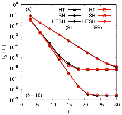
Figure 1: Approach to steady state, assessed at the level of the temperature profile, at (a) $\delta=10$, (b) $\delta=1$ and (c) $\delta=0.1$. The results for heat transfer under stationary walls (HT), Couette flow (SH) and heat transfer under shear (HTSH) are represented using squares, circles and rhombi, respectively. The results for the S and ES models are represented using black lines with filled symbols and red lines with empty symbols, respectively.

It is known that the DSMC method suffers from stochastic noise, which persists after the steady state is reached. This noise can be eliminated through averaging over a large number of time steps, which can be time consuming especially at large values of $\delta$. The time required to complete the DSMC simulations in this paper is about $20$ hours using an MPI parallel code which runs on 32 processor cores.

In the case of the kinetic solver, we estimate the computational efficiency by considering simulations on a single core of an i7-4790K processor, running at a frequency of $4.0\ {\rm GHz}$. The simulation time is very short at $\delta=10$ and $\delta=1$ – of the order of one minute. This is because the quadrature order employed can be very small. At $\delta=0.1$, the quadrature must be increased, leading to computational times of the order of $5$–$10$ minutes on a single processor core. The exact figures are summarised in Table 2. For completeness, in this table we included also the simulation times required to reach the stationary states when using the hybrid approach at $\delta=100$ and $1000$, corresponding to the hydrodynamics regime. It can be seen that the hybrid approach described in this section becomes inefficient when $\delta$ increases. This happens because, for $\delta\gtrsim 10$, the number of iterations required to reach the steady state increases dramatically with $\delta$, being around two orders of magnitude larger at $\delta=1000$ than at $\delta=10$. It is noteworthy that the projection method discussed in A performs better at larger values of $\delta$, as can be seen in Table 3. In particular, the computing times required by the projection method at $\delta=1000$ are shorter than those required by the hybrid method by factors of about $4$ and $5$ for the S and ES models, respectively. Further decreases in computational time at large values of $\delta$ can be expected when the explicit time-stepping method employed in this paper is replaced by, e.g., the implicit-explicit (IMEX) method that treats the collision term implicitly [98, 99, 100], or the iterative methods discussed in Refs. [72, 73, 74, 75].

Before ending this section, we briefly mention the procedure employed to judge the approach to steady state. We consider 10 batches of $N_{T}$ iterations each, with a time step of $\delta t$. The time interval corresponding to one batch is $\Delta t=N_{T}\delta t$. Denoting via $T^{n}(x)$ the temperature profile after the $n$th batch, we compute the $L_{2}$ norm of the relative difference between two successive batches, as follows:

$$L_{2}[T^{n+1}]=\left[\frac{1}{\widetilde{L}}\int_{-\widetilde{L}/2}^{\widetilde{L}/2}d\widetilde{x}\,\left(\frac{\widetilde{T}^{n+1}(\widetilde{x})}{\widetilde{T}^{n}(\widetilde{x})}-1\right)^{2}\right]^{1/2},$$ (107)

where the integration is performed as indicated in Eqs. (105) and (106). Figure 1 shows that $L_{2}[T]$ steadily decreases with the time $t$ ($t_{n}=n\Delta t$).

Figure 2: The simulation setup for the heat transfer problem. The vertical dashed lines show a sample grid employing $S=4$ points on each half of the channel, stretched according to Eq. (43) with $A=0.95$.

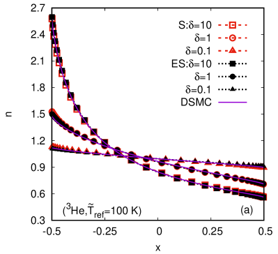
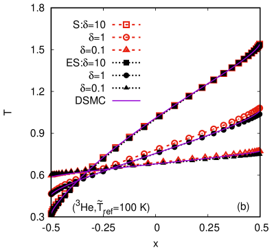
Figure 3: Comparison between the S (red dashed lines and empty symbols) and ES (black dotted lines and filled symbols) results and the DSMC (continuous lines) results in the context of the heat transfer between stationary plates problem for the profiles of (a) $n$ and (b) $T$ through the channel ($-1/2\leq x\leq 1/2$), for ${}^{3}{\rm He}$ gas constituents. The reference temperature is set to $\widetilde{T}_{\rm ref}=100\ {\rm K}$, while the temperature difference between the two walls is $\widetilde{\Delta T}=1.5\widetilde{T}_{\rm ref}$.

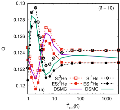
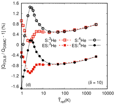
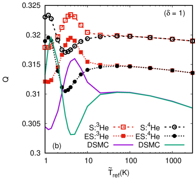
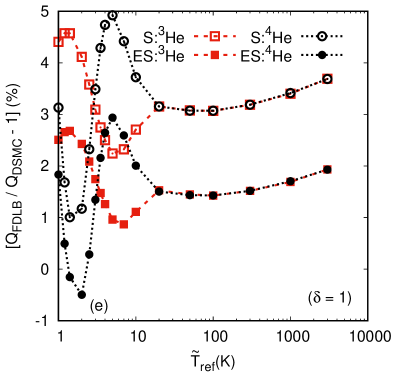
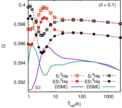
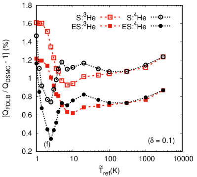
Figure 4: (Left) Dependence of the constant $Q$, computed for the heat transfer between stationary plates problem using Eq. (99) with $\widetilde{u}_{y}=0$, on the average wall temperature $\widetilde{T}_{\rm ref}$. (Right) Relative error $Q_{\rm FDLB}/Q_{\rm DSMC}-1$ of the FDLB results with respect to the DSMC results. Both ${}^{3}{\rm He}$ (red dashed lines with squares) and ${}^{4}{\rm He}$ (black dotted lines with circles) are considered within the S (empty symbols) and ES (filled symbols) models and the results are represented at $\delta=10$ (top), $1$ (middle) and $0.1$ (bottom).

5 Heat transfer

The first application considered in this paper concerns the heat transfer between stationary parallel plates problem. The simulation setup is represented schematically in Fig. 2. In our simulations, the reference temperature, $\widetilde{T}_{\rm ref}=(\widetilde{T}_{\rm left}+\widetilde{T}_{\rm right})/2$, is varied between $1\ {\rm K}$ and $3000\ {\rm K}$.

Representative profiles of the density $n$ and temperature $T$ are shown for ${}^{3}{\rm He}$ constituents at $\widetilde{T}_{\rm ref}=100\ {\rm K}$ in Fig. 3. The DSMC results are shown using solid lines. The FDLB results obtained with the S model are shown using red dashed lines with empty symbols. The FDLB results obtained with the ES model are shown using black dotted lines with filled symbols. The FDLB data corresponding to $\delta=10$, $1$ and $0.1$ are shown with squares, circles and triangles, respectively. Very good agreement can be seen between the results obtained using the ES model and the DSMC data. There is a visible discrepancy in the temperature profile obtained with the Shakohv model at $\delta=1$.

A more quantitative analysis is performed at the level of the quantity $Q$, introduced in Eq. (99), with $\widetilde{u}_{y}$ set to $0$. Figure 4 compares the FDLB and DSMC results for $Q$ with respect to $\widetilde{T}_{\rm ref}$ for $1\ {\rm K}\leq\widetilde{T}_{\rm ref}\leq 3000\ {\rm K}$, at $\delta=10$ (top line), $1$ (middle line) and $0.1$ (bottom line). The value of $Q$ is represented in the left column of Fig. 4, while the relative error $Q_{\rm FDLB}/Q_{\rm DSMC}-1$ is shown in the right column of Fig. 4. These results were obtained using the S (empty symbols) and the ES (filled symbols) models, for both the ${}^{3}{\rm He}$ (red lines with squares) and the ${}^{4}{\rm He}$ (black lines with circles) constituents. At $\delta=10$, the S model overestimates the DSMC results. Contrary to the S model, these DSMC results are underestimated by the ES model. The relative errors are roughly the same in absolute values. At smaller values of $\delta$, the ES model provides results which are more accurate than those obtained using the S model. The highest relative discrepancy with respect to the DSMC data can be observed at $\delta=1$, when the relative error of the S model reaches almost $5\%$, while for the ES model, it stays below $3\%$.

6 Couette flow

Figure 5: The simulation setup for the Couette flow problem. The vertical dashed lines show a sample grid employing $S=8$ points, stretched according to Eq. (43) with $A=0.95$.

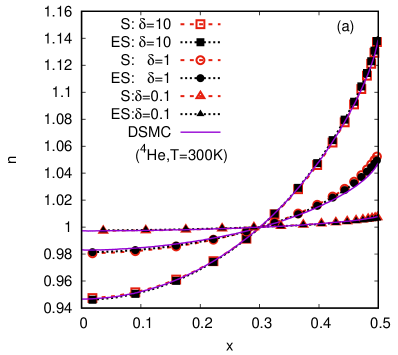
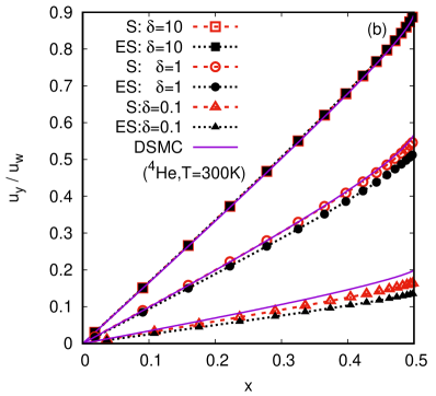
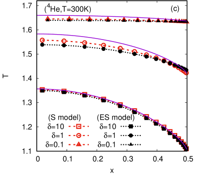
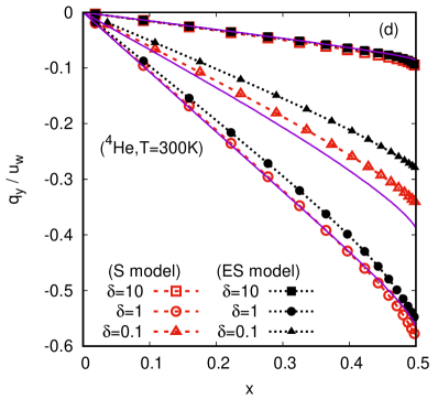
Figure 6: Comparison between the FDLB results for the S model (dashed red lines and empty symbols) and ES model (dotted black lines and filled symbols) and the DSMC results (continuous lines) for the profiles of (a) $n$, (b) $u_{y}$, (c) $T$ and (d) $q_{y}$ through the half-channel ($0\leq x\leq 1/2$), for ${}^{4}{\rm He}$ gas constituents, in the context of the Couette flow. The wall temperature is set to $\widetilde{T}_{\rm ref}=300\ {\rm K}$, while the wall velocity is $u_{w}=\sqrt{2}$.

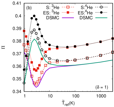
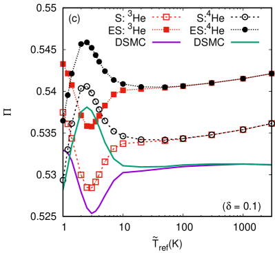
Figure 7: Dependence of $\Pi$, computed using Eq. (98) in the context of the Couette flow, on the wall temperature $\widetilde{T}_{\rm ref}$ for both ${}^{3}{\rm He}$ (squares) and ${}^{4}{\rm He}$ (circles), at (a) $\delta=10$, (b) $\delta=1$ and (c) $\delta=0.1$.

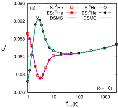
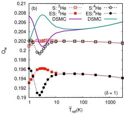
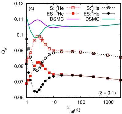
Figure 8: Dependence of $Q_{w}$, computed in the context of the Couette flow using Eq. (103), on the wall temperature $\widetilde{T}_{\rm ref}$ for both ${}^{3}{\rm He}$ (squares) and ${}^{4}{\rm He}$ (circles), at (a) $\delta=10$, (b) $\delta=1$ and (c) $\delta=0.1$.

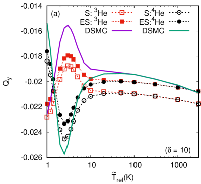
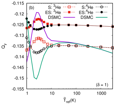
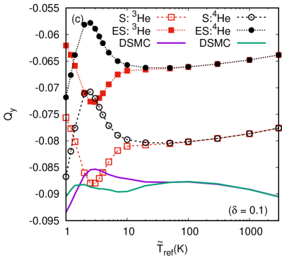
Figure 9: Dependence of $Q_{y}$, computed in the context of the Couette flow using Eq. (102), on the wall temperature $\widetilde{T}_{\rm ref}$ for both ${}^{3}{\rm He}$ (squares) and ${}^{4}{\rm He}$ (circles), at (a) $\delta=10$, (b) $\delta=1$ and (c) $\delta=0.1$.

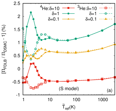
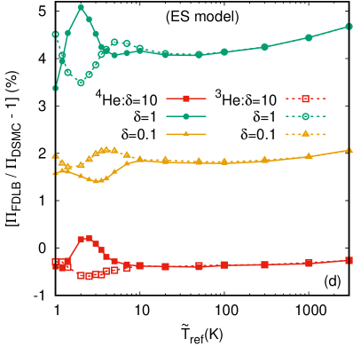
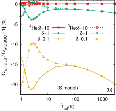
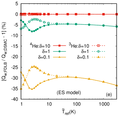
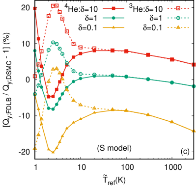
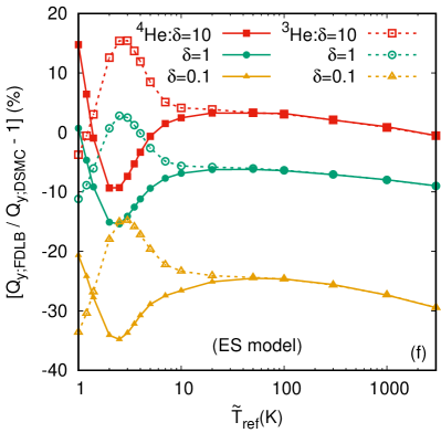
Figure 10: Relative errors $\Pi_{\rm FDLB}/\Pi_{\rm DSMC}-1$ (top), $Q_{w;{\rm FDLB}}/Q_{w;{\rm DSMC}}-1$ (middle) and $Q_{y;{\rm FDLB}}/Q_{y;{\rm DSMC}}-1$ (bottom) between the DSMC and FDLB results for the S model (left) and ES model (right), at $\delta=10$ (squares), $1$ (circles) and $0.1$ (triangles) for $1\ {\rm K}\leq\widetilde{T}_{\rm ref}\leq 3000\ {\rm K}$, computed in the context of the Couette flow.

The second application concerns the Couette flow between parallel plates. Due to the symmetry of the flow, only the right half of the channel ($0\leq x\leq 1/2$) is considered in the simulation setup, as shown in Fig. 5. The walls are kept at constant temperatures $\widetilde{T}_{\rm left}=\widetilde{T}_{\rm right}=\widetilde{T}_{\rm ref}$ and $\widetilde{T}_{\rm ref}$ is varied bewteen $1\ {\rm K}$ and $3000\ {\rm K}$. The wall velocity $\widetilde{u}_{w}=\sqrt{2\widetilde{K}_{B}\widetilde{T}_{\rm ref}/\widetilde{m}}$ takes the value $u_{w}=\sqrt{2}$ after non-dimensionalization.

Aside from the transversal component $q_{x}$ of the heat flux, which can be related at large $\delta$ to the temperature variations with respect to the coordinate $x$ via Fourier’s law, $q_{x}=-\kappa\partial_{x}T$, the Couette flow exhibits a non-vanishing longitudinal heat flux, $q_{y}$, which is a purely microfluidics effect. Figure 6 shows a comparison between the FDLB results for the S (dashed red lines and empty symbols) and ES (dotted black lines and filled symbols) models and the DSMC results (solid purple lines). The wall temperature is set to $\widetilde{T}_{\rm ref}=300\ {\rm K}$ and ${}^{4}{\rm He}$ gas constituents are considered for $\delta=10$, $1$ and $0.1$. Both the S and ES models are in good agreement with the DSMC data at $\delta=10$. When $\delta$ decreases, the agreement deteriorates, being slightly worse in the case of the ES model. Remarkably, the density profiles are well recovered with both models at all tested values of $\delta$.

We now consider a more quantitative analysis at the level of $\Pi$, $Q_{w}$ and $Q_{y}$, computed via Eqs. (96), (103) and (102), respectively. The variations with the plate temperature $\widetilde{T}_{\rm ref}$ of $\Pi$, $Q_{w}$ and $Q_{y}$ for ${}^{3}{\rm He}$ and ${}^{4}{\rm He}$ are shown in Figs. 7, 8 and 9 for (a) $\delta=10$, (b) $\delta=1$ and (c) $\delta=0.1$. Each plot shows curves corresponding to the S model (dashed lines with empty symbols), ES model (dotted lines with filled symbols) and DSMC (solid lines). The data corresponding to ${}^{3}{\rm He}$ is shown using red squares, while the data for ${}^{4}{\rm He}$ is shown with black circles. It can be seen that in general, the agreement between the results obtained with the model equations and the DSMC results deteriorates as $\delta$ is decreased. Contrary to the results obtained in the case of the heat transfer problem, the S model gives more accurate results compared to the ES model, confirming the results reported in Ref. [89]. Figure 10 shows the relative errors computed with respect to the DSMC results, obtained with the S (left column) and ES (right column) models. The results for ${}^{4}{\rm He}$ are shown with solid lines and filled symbols, while those for ${}^{3}{\rm He}$ are shown with dashed lines and empty symbols. The data corresponding to $\delta=10$, $1$ and $0.1$ are shown with red squares, green circles and amber triangles, respectively. In the case of $\Pi$, the relative error of the ES model is roughly twice that of the S model.

It is remarkable that the relative errors for both $Q_{w}$ and $Q_{y}$ (shown in Figs. 8 and 9) reach values around $20\%$ for $\delta=0.1$. This can be explained since the heat fluxes decrease to $0$ as $\delta$ is decreased, while $\Pi$, for which the relative error is below $5\%$, attains a finite value as the ballistic regime is approached ($\lim_{\delta\rightarrow 0}\Pi=\pi^{-1/2}$). Thus, the relative errors for $Q_{w}$ and $Q_{y}$ are computed by dividing the FDLB values by small numbers. However, in the case of $Q_{y}$, the errors are around $20\%$ even when $\delta=10$, whereas for both $Q_{w}$ and $\Pi$, the error at $\delta=10$ is less than $1\%$. This disagreement between the model equations and the DSMC data can be attributed to the nature of $Q_{y}$. Since the longitudinal heat flux, $q_{y}$, is not generated by a temperature gradient (through the so-called direct phenomenon), its characteristics must depend on higher order transport coefficients, which are visible only at the Burnett level [101]. Since the model equations are constructed to ensure consistency only at the Navier-Stokes level (corresponding to the first order in the Chapman-Enskog expansion), it is not surprising that such cross phenomena are not accurately recovered.

7 Heat transfer under shear

Figure 11: The simulation setup for the heat transfer under shear problem. The vertical dashed lines show a sample grid employing $S=4$ points on each half of the channel, stretched according to Eq. (43) with $A=0.95$.

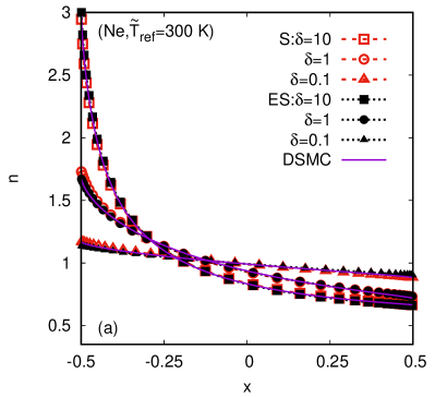
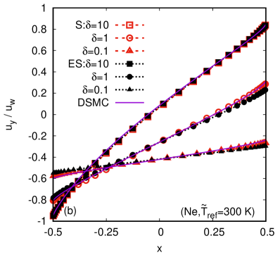
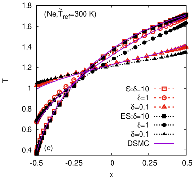
Figure 12: Comparison between the FDLB results (dotted lines and points) obtained using the S (red empty symbols) and ES (black filled symbols) models and the DSMC (continuous lines) results for the profiles of $n$ (a), $u_{y}$ (b) and $T$ (c) through the channel ($-1/2\leq x\leq 1/2$), for ${\rm Ne}$ gas constituents, in the context of the heat transfer between moving plates problem. The reference temperature is set to $\widetilde{T}_{\rm ref}=300\ {\rm K}$, the temperature difference between the two walls is $\widetilde{\Delta T}=1.5\widetilde{T}_{\rm ref}$ and the wall velocity is $\widetilde{u}_{w}=\sqrt{2\widetilde{K}_{B}\widetilde{T}_{\rm ref}/\widetilde{m}}$.

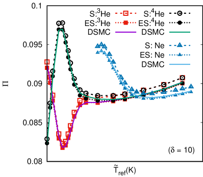
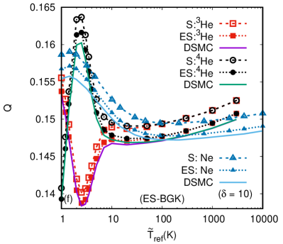
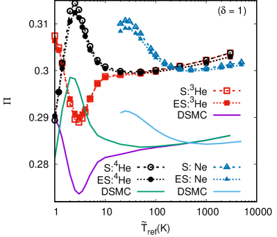
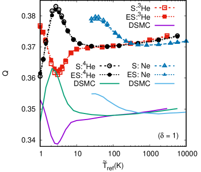
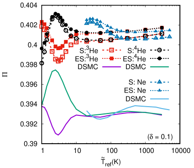
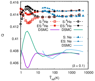
Figure 13: Dependence of $\Pi$ (left column) and $Q$ (right column), defined in Eqs. (96) and (99) for the heat transfer between moving plates problem, on the average wall temperature $\widetilde{T}_{\rm ref}=(\widetilde{T}_{\rm left}+\widetilde{T}_{\rm right})/2$ for ${}^{3}{\rm He}$ (red squares), ${}^{4}{\rm He}$ (black circles) and ${\rm Ne}$ (blue triangles), at $\delta=10$ (top line), $1$ (middle line) and $0.1$ (bottom line).

The final example considered in this paper is the heat transfer between parallel plates in motion. The simulation setup is represented in Fig. 11. This example combines the features of the heat transfer between stationary plates discussed in Sec. 5 and those of the Couette flow discussed in Sec. 6. The reference temperature $\widetilde{T}_{\rm ref}=(\widetilde{T}_{\rm left}+\widetilde{T}_{\rm right})/2$, is varied between $1\ {\rm K}$ and $3000\ {\rm K}$ for ${}^{3}{\rm He}$ and ${}^{4}{\rm He}$ constituents, while for ${\rm Ne}$, the range for $\widetilde{T}_{\rm ref}$ is $20\ {\rm K}\leq\widetilde{T}_{\rm ref}\leq 5000\ {\rm K}$. As in Sec. 5, the temperature difference $\widetilde{\Delta T}=\widetilde{T}_{\rm right}-\widetilde{T}_{\rm left}$ obeys Eq. (100). Furthermore, the plates have velocities $\widetilde{\bm{u}}_{\rm left}=-\widetilde{u}_{w}\bm{j}$ and $\widetilde{\bm{u}}_{\rm right}=\widetilde{u}_{w}\bm{j}$, where $\widetilde{u}_{w}=\sqrt{2\widetilde{K}_{B}\widetilde{T}_{\rm ref}/\widetilde{m}}$, such that the Mach number is given by Eq. (97).

Figure 12 shows the profiles of the density (a), velocity (b) and temperature (c) for the case of ${\rm Ne}$ constituents at $T=300\ {\rm K}$. In general, good agreement can be seen between the results corresponding to the model equations and the DSMC results. A larger discrepancy can be seen between the ES model and the DSMC results, especially in the temperature profile at $\delta=1$ and $0.1$.

A quantitative analysis can be made at the level of the nondimensional quantities $\Pi$ and $Q$, computed using Eqs. (96) and (99). Figure 13 shows a comparison between the FDLB results for the S (dashed lines with empty symbols) and the ES (dotted lines with filled symbols) models and the DSMC results (solid lines), obtained for ${}^{3}{\rm He}$ (squares), ${}^{4}{\rm He}$ (circles), and ${\rm Ne}$ (triangles) constituents. Figure 14 shows the relative errors in $Q$ (dashed lines and empty symbols) and $\Pi$ (dotted lines and filled symbols) computed for the S model (left column) and ES model (right column) with respect to the DSMC results for ${}^{3}{\rm He}$ (squares), ${}^{4}{\rm He}$ (circles) and ${\rm Ne}$ (triangles). At $\delta=10$ (top line), the results obtained using the ES model seem to be in better agreement with the DSMC results than those obtained using the S model. At $\delta=1$ (middle line) and $0.1$ (bottom line), the two models give results with similar accuracy. As noticed in the case of the heat transfer between stationary plates and in the case of the direct phenomena in the Couette flow, the relative erros are highest at $\delta=1$, where they take values between $6-8\%$ (about $1\%$ higher for $Q$ than for $\Pi$).

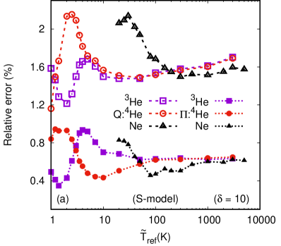
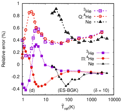
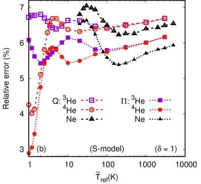
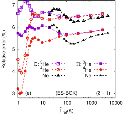
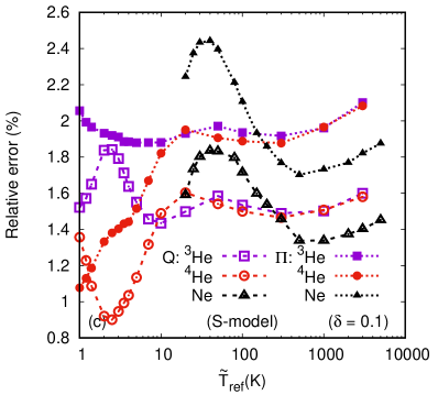
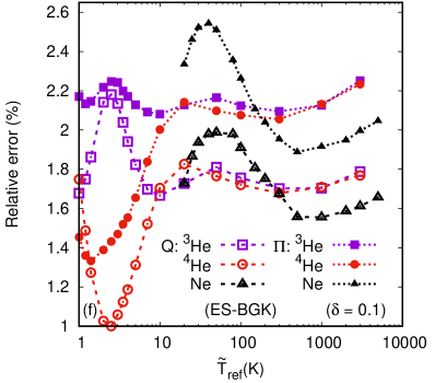
Figure 14: Dependence of the relative errors $Q_{\rm FDLB}/Q_{\rm DSMC}-1$ (dashed lines and empty symbols) and $\Pi_{\rm FDLB}/\Pi_{\rm DSMC}-1$ (dotted lines and filled symbols), expressed in percentages, where the FDLB results are obtained using the S (left column) and ES (right column) models, for the heat transfer between moving plates problem, on the average wall temperature $T_{\rm ref}=(T_{\rm left}+T_{\rm right})/2$ for ${}^{3}{\rm He}$ (squares), ${}^{4}{\rm He}$ (circles) and ${\rm Ne}$ (triangles), at $\delta=10$ (top line), $1$ (middle line) and $0.1$ (bottom line).

8 Conclusion

In this paper, we presented a systematic comparison between the results obtained using the Boltzmann equation with the Shakhov (S) and Ellipsoidal-BGK (ES) models for the collision term and those obtained using the direct simulation Monte Carlo (DSMC) method for three benchmark channel flows between parallel plates, namely: heat transfer between static walls, Couette flow and heat transfer under shear. The results were obtained numerically in the nonlinear regime [${\rm Ma}\simeq 2.19$ for the case when the parallel plates are moving and $2(\widetilde{T}_{\rm right}-\widetilde{T}_{\rm left})/(\widetilde{T}_{\rm right}+\widetilde{T}_{\rm left})=1.5$ for the heat transfer problems], by considering ${}^{3}{\rm He}$ and ${}^{4}{\rm He}$ constituents interacting via ab initio potentials. We also considered ${\rm Ne}$ constituents for the heat transfer under shear problem.

In the kinetic theory setup, the connection with the DSMC simulations was established at the level of the transport coefficients (dynamic viscosity $\widetilde{\mu}$ and heat conductivity $\widetilde{\kappa}$). For ${}^{3}{\rm He}$ and ${}^{4}{\rm He}$, the range of values for the reference temperature $\widetilde{T}_{\rm ref}=(\widetilde{T}_{\rm right}+\widetilde{T}_{\rm left})/2$ was $1\ {\rm K}\leq\widetilde{T}_{\rm ref}\leq 3000\ {\rm K}$, while for the ${\rm Ne}$ constituents, it was $20\ {\rm K}\leq\widetilde{T}_{\rm ref}\leq 5000\ {\rm K}$. We considered three values for the rarefaction parameter, namely $\delta=10$ (slip flow regime), $\delta=1$ (transition regime) and $\delta=0.1$ (early free molecular flow regime).

We first conducted a qualitative comparison at the level of the profiles of the density, temperature, velocity and heat flux. In all cases considered, the density profile was well recovered with both kinetic models, for all values of the rarefation parameter. In the context of the heat transfer problem, the results obtained using the ES model were in better agreement with the DSMC results for the temperature profile. In the Couette and heat transfer with shear problems, the S model seemed to give results which were closer to the DSMC predictions for all quantities (temperature, velocity and heat flux).

We next considered a quantitative comparison of the performance of the kinetic models with respect to the DSMC data by comparing the numerical values for non-dimensional quantities derived from the longitudinal heat flux (in the case of heat transfer between stationary and moving plates, denoted $Q$), shear stress (in the case of Couette flow and heat transfer between moving plates, denoted $\Pi$), as well as the half-channel heat flow rate, $Q_{y}$, and heat transfer rate through the boundary, $Q_{w}$ (in the case of the Couette flow). Among these quantities, we can distinguish two categories. The first category (containing $Q$, $\Pi$ and $Q_{w}$) refers to quantities related to “direct phenomena,” which are driven by, e.g., shear rate $\partial_{x}u_{y}$ for $\Pi$ and temperature gradient $\partial_{x}T$ for $Q$, as predicted by the Navier-Stokes-Fourier theory. The second category (containing $Q_{y}$) refers to quantities related to “cross phenomena,” visible at the level of the Burnett equations, in which the usual thermodynamic forces driving the non-equilibrium quantity are absent (i.e., non-vanishing $q_{y}$ when $\partial_{y}T=0$).

For the quantities in the first category (corresponding to direct phenomena), the agreement between the kinetic models and the DSMC results was within a few percent at $\delta=10$, which confirms the validity of these models in the slip flow regime. At $\delta=1$, the errors seem to be bounded within $8\%$ for both models, with the ES model giving better results in the heat transfer between stationary plates problem, while the S model performs better for the Couette flow and heat transfer under shear problems. When $\delta=0.1$, the free molecular flow regime is approached. For the quantities that attain a finite value in this regime ($Q$ in the heat transfer problems and $\Pi$ in the Couette flow problem), the relative errors drop compared to $\delta=1$, to within $2\%-3\%$. On the contrary, the relative errors for the heat flux $Q_{w}$ measured at the wall in the Couette flow grow to around $20\%$ for the S model and $30\%$ for the ES model. This can be attributed to the fact that $Q_{w}$ decreases towards $0$ as the free molecular flow regime is approached, such that the relative errors are computed by dividing the results obtained within the model equations by a small quantity.

When considering the quantity $Q_{y}$ from the second category, which is generated through the cross-phenomena, the results of the kinetic models had relative errors of the order of $20\%$ even at $\delta=10$, highlighting that the model equations do not accurately take into account such phenomena. At $\delta=1$, the relative errors decrease to around $10\%$ for the S model and $15\%$ for the ES model. At $\delta=0.1$, they increase again to around $20\%$ and $35\%$ for the S and ES models, respectively. As was the case for $Q_{w}$, the large values of the relative errors of $Q_{y}$ encountered at $\delta=10$ and $\delta=0.1$ may be caused by the fact that $Q_{y}$ vanishes in the inviscid ($\delta\rightarrow\infty$) and free molecular flow ($\delta\rightarrow 0$) regimes.

In conclusion, our results demonstrate that even in the strongly non-linear regime, the model equations can give reasonably accurate results, with errors of up to $10\%$ for quantities related to direct phenomena throughout the rarefaction spectrum (provided they remain finite in the free molecular flow regime), while the errors for the cross phenomena-related quantities seem to be within $35\%$. Due to the computational efficiency of the finite difference lattice Boltzmann (FDLB) algorithm employed in this paper, solving the kinetic model equations can provide a cheap and reasonably accurate solution for the flow properties in the case of realistic monatomic gases under rarefied conditions.

Acknowledgments. VEA gratefully acknowledges the generous support of the Romanian-U.S. Fulbright Commission through The Fulbright Senior Postdoctoral Program for Visiting Scholars 2017-2018, Grant number 678/2018. FS acknowledges the Brazilian Agency CNPq, Brazil, for the support of his research, grant 304831/2018-2. VEA is grateful to Professor P. Dellar (Oxford University, UK) for preliminary discussions regarding the projection of the Shakhov collision term onto orthogonal polynomials. The numerical simulations were performed on the Turing High Performance Computing cluster and the Computing cluster at the Computer Science Department of the Old Dominion University (Norfolk, VA, USA). The computer simulations reported in this paper were done using the Portable Extensible Toolkit for Scientific Computation (PETSc 3.6) developed at Argonne National Laboratory, Argonne, Illinois [102, 103].

Appendix A FDLB models for the hydrodynamic regime

When $\delta\gtrsim 100$, the flow enters the hydrodynamic regime, where it can be approximately described by the Navier-Stokes equations [104],

$$\frac{D\rho}{Dt}+\rho\nabla\cdot\bm{u}= 0,$$

$$\rho\frac{Du_{i}}{Dt}+\partial_{i}P= -\partial_{j}\sigma_{ij},$$

$$\rho\frac{De}{Dt}+P\nabla\cdot\bm{u}= -\sigma_{ij}\partial_{i}u_{j}-\nabla\cdot\bm{q},$$ (108)

where $D/Dt=\partial_{t}+\bm{u}\cdot\nabla$ is the convective (material) derivative, $\sigma_{ij}=T_{ij}-P\delta_{ij}$ is the shear stress tensor, $\bm{q}$ is the heat flux, $e=\frac{3}{2m}T$ is the specific energy for an ideal monatomic gas. The Newtonian fluid model and Fourier’s law give the following constitutive equations for $\tau_{ij}$ and $\bm{q}$:

$$\tau_{ij}=-\mu\left(\partial_{i}u_{j}+\partial_{j}u_{i}-\frac{2}{3}\delta_{ij}\nabla\cdot\bm{u}\right),\qquad\bm{q}=-\kappa\nabla T,$$ (109)

where $\mu$ and $\kappa$ are the dynamic viscosity and heat conductivity, respectively.

According to the Chapman-Enskog expansion, briefly discussed in A.1, low order moments of the reduced distribution functions $\phi$ and $\chi$ are required to ensure the relations in Eq. (109). The evolution and stationary state properties of these moments can be obtained by employing similarly low order quadratures (i.e., $Q_{x}^{\phi}=5$ and $Q_{y}^{\phi}=4$ for the $\phi$ distribution; and $Q_{x}^{\chi}=3$ and $Q_{y}^{\chi}=2$ for the $\chi$ distribution).

As the quadrature order is lowered and $\delta$ is increased, the recovery of the conservation equations becomes increasingly challenging when the distributions are evaluated directly (i.e., using the hybrid method described in Sec. 3.3). In the traditional lattice Boltzmann framework, the key to employing the low order quadratures is to project the local equilibrium distribution on a set of orthogonal polynomials, which is subsequently truncated at an order $N_{x}^{*}$ ($*\in\{\phi,\chi\}$).

A.1 Chapman-Enskog analysis

To derive the hydrodynamic regime from the kinetic model equation,

$$\frac{\partial f}{\partial t}+\frac{\bm{p}}{m}\cdot\nabla f=-\frac{1}{\tau_{*}}(f-f_{*}),$$ (110)

the fluid can be assumed to be very close to isotropic thermal equilibrium, described by $f=f_{*}=f^{\rm{(eq)}}$, where $f^{\rm{(eq)}}$ is the Maxwell-Boltzmann distribution. The deviations of $f$ and $f_{*}$ from $f^{\rm{(eq)}}$, denoted by $\delta f=f-f^{\rm{(eq)}}$ and $\delta f_{*}=f_{*}-f^{\rm{(eq)}}$, can be assumed to be of the same order as the relaxation time $\tau_{*}$, which is considered to be small. To first order with respect to $\tau_{*}$, the deviation $\delta f$ can be written as

$$\delta f=\delta f_{*}-\tau_{*}\left(\frac{\partial f^{\rm{(eq)}}}{\partial t}+\frac{\bm{p}}{m}\cdot\nabla f^{\rm{(eq)}}\right),$$ (111)

where $f^{\rm{(eq)}}$ is determined by the density $\rho$, velocity $\bm{u}$ and temperature $T$. The constitutive relations for $\sigma_{ij}=T_{ij}-P\delta_{ij}$ and $q_{i}$ given in Eq. (109) can be obtained by taking the second and third order moments of Eq. (111) with respect to the momentum space:

$$\sigma_{ij}= \sigma^{*}_{ij}-\tau_{*}\left(\frac{\partial}{\partial t}\int d^{3}p\,\frac{p_{i}p_{j}}{m}f^{\rm{(eq)}}+\partial_{k}\int d^{3}p\,\frac{p_{i}p_{j}p_{k}}{m^{2}}f^{\rm{(eq)}}\right),$$

$$q_{i}+u_{j}\sigma_{ij}= q_{i}^{*}+u_{j}\sigma^{*}_{ij}-\tau_{*}\left(\frac{\partial}{\partial t}\int d^{3}p\,\frac{\bm{p}^{2}p_{i}}{2m^{2}}f^{\rm{(eq)}}+\partial_{k}\int d^{3}p\,\frac{\bm{p}^{2}p_{i}p_{k}}{2m^{3}}f^{\rm{(eq)}}\right),$$ (112)

where $\sigma^{*}_{ij}$ and $q_{i}^{*}$ are obtained by taking moments of $\delta f_{*}$,

$$\int d^{3}p\,\frac{p_{i}p_{j}}{m}\delta f_{*}=\sigma^{*}_{ij},\qquad\int d^{3}p\,\frac{\bm{p}^{2}p_{i}}{2m^{2}}\delta f_{*}=q_{i}^{*}+\sigma^{*}_{ij}u_{j}.$$ (113)

For completeness, the details of the Chapman-Enskog procedure for the S and ES models employed in this paper are briefly presented. The integrals of $f^{\rm{(eq)}}$ entering Eq. (112) are

$$\int d^{3}p\,\frac{p_{i}p_{j}}{m}f^{\rm{(eq)}}= P\delta_{ij}+\rho u_{i}u_{j},$$

$$\int d^{3}p\,\frac{p_{i}p_{j}p_{k}}{m^{2}}f^{\rm{(eq)}}= P(\delta_{ij}u_{k}+\delta_{jk}u_{i}+\delta_{ki}u_{j})+\rho u_{i}u_{j}u_{k},$$

$$\int d^{3}p\,\frac{\bm{p}^{2}p_{i}}{2m^{2}}f^{\rm{(eq)}}= \frac{5P}{2}u_{i}+\frac{\rho\bm{u}^{2}}{2}u_{i},$$

$$\int d^{3}p\,\frac{\bm{p}^{2}p_{i}p_{k}}{2m^{3}}f^{\rm{(eq)}}= P\left(\frac{5T}{2m}+\frac{\bm{u}^{2}}{2}\right)\delta_{ik}+\left(\frac{7P}{2}+\frac{\rho\bm{u}^{2}}{2}\right)u_{i}u_{k}.$$ (114)

Using the above relations and replacing the time derivatives using the Euler (inviscid) form of the Navier-Stokes equations (108),

$$\frac{D\rho}{Dt}+\rho\nabla\cdot\bm{u}=O(\tau_{*}),\qquad\rho\frac{D\bm{u}}{Dt}+\nabla P=O(\tau_{*}),\qquad\rho\frac{De}{Dt}+P\nabla\cdot\bm{u}=O(\tau_{*}),$$ (115)

it can be seen that

$$\sigma_{ij}= \sigma^{*}_{ij}-\tau_{*}P\left(\partial_{i}u_{j}+\partial_{j}u_{i}-\frac{2}{3}\nabla\cdot\bm{u}\delta_{ij}\right), \bm{q}= \bm{q}_{*}-\frac{5\tau_{*}P}{2m}\nabla T.$$ (116)

In the Shakhov (S) and ellipsoidal (ES) models, when $f_{*}$ are given by $f_{\rm S}$ and $f_{\rm ES}$ introduced in Eqs. (4) and (7), $\sigma^{*}_{ij}$ and $\bm{q}_{*}$ are given by:

$$\sigma^{\rm S}_{ij}= 0, \bm{q}_{\rm S}= (1-{\rm Pr})\bm{q},$$

$$\sigma^{\rm ES}_{ij}= -\frac{1-{\rm Pr}}{\rm Pr}\sigma_{ij}, \bm{q}_{\rm ES}= 0.$$ (117)

Substituting Eq. (117) into Eq. (116) and comparing the result to Eq. (109), the relations given in Eqs. (6) and (10) between the relaxation times, $\tau_{\rm S}$ and $\tau_{\rm ES}$, and the transport coefficients $\mu$ and $\kappa$ can be obtained.

The recovery of the constitutive equations (109) is conditioned by the correct recovery of the integrals (113) and (114) of $f_{*}$ and $f^{\rm{(eq)}}$.

In the case when the flow is trivial along the $z$ direction ($d=2$), the $p_{z}$ degree of freedom can be integrated automatically and Eqs. (114) and (113) can be written in terms of the reduced distributions $\phi$ and $\chi$ introduced in Eq. (14). The highest moments required for the reduced equilibrium distributions $\phi_{*}$ and $\chi_{*}$ are derived from the fourth order moment on the last line of Eq. (114). Substituting $f^{\rm{(eq)}}\rightarrow f_{*}$, the following equation is obtained:

$$\int d^{3}p\,\frac{\bm{p}^{2}p_{i}p_{k}}{2m^{3}}f_{*}=\int dp_{x}\,dp_{y}\left[\frac{(p_{x}^{2}+p_{y}^{2})p_{i}p_{k}}{2m^{3}}\phi_{*}+\frac{p_{i}p_{k}}{2m^{2}}\chi_{*}\right].$$ (118)

It can be seen that the above integrals require the correct recovery of the moments with respect to $p_{x}$ of order $4$ for $\phi_{*}$ and of order $2$ for $\chi_{*}$. This can be achieved using the half-range Gauss-Hermite quadrature employing $Q_{x}^{\phi}=5$ and $Q_{x}^{\chi}=3$ points on each of the $p_{x}>0$ and $p_{x}<0$ semiaxes. Furthermore, $\phi_{*}$ and $\chi_{*}$ must be replaced by a truncated expansion with respect to the half-range Hermite polynomials of orders $Q_{x}^{*}-1$. More details for each of the collision models are given below.

A.2 Maxwell-Boltzmann distribution

The projection of the Maxwell-Boltzmann distribution $f^{\rm{(eq)}}$ with respect to the half-range Gauss-Hermite polynomials was derived in Ref. [44]. Here, we only summarise the details. Considering the factorisation $f^{\rm{(eq)}}=ng_{x}g_{y}g_{z}$ introduced in Eq. (2), the expansion of $f^{\rm{(eq)}}$ can be performed at the level of each $g_{i}$ factor individually. Specifically, the $g_{z}$ factor is integrated out when introducing the reduced distributions. The $g_{y}$ factor is expanded up to order $N_{y}^{*}$ ($*\in\{\phi,\chi\}$) with respect to the full-range Hermite polynomials, as summarised in Eqs. (80)–(81) and (90)–(91) in the contexts of the ES and S models. For the Maxwell-Boltzmann distribution, Eqs. (80) and (81) can be used by substituting $\zeta_{y}$ and $T_{y}$ by $u_{y}$ and $T$, respectively.

The $g_{x}$ factor is expanded with respect to the half-range Hermite polynomials up to orders $N_{x}^{\phi}=Q_{x}^{\phi}-1=4$ and $N_{x}^{\chi}=Q_{x}^{\chi}-1=2$:

$$g^{(N_{x}^{*})}(p_{x},u_{x},T)=\frac{\omega(\overline{p}_{x})}{p_{0,x}}\sum_{r=0}^{N_{x}^{*}}\mathfrak{h}_{r}(|\overline{p}_{x}|)[\theta(p_{x})\mathcal{G}^{+}_{r}(u_{x},T)+\theta(-p_{x})\mathcal{G}^{-}_{r}(u_{x},T)],$$ (119)

where $\theta(x)$ is the Heaviside step function. The coefficients $\mathcal{G}^{\pm}_{r}$ are given by

$$\mathcal{G}^{\pm}_{r}(u_{x},T)=\frac{1}{2}\sum_{s=0}^{r}(\pm 1)^{s}\mathfrak{h}_{r,s}\left(\frac{mT}{2p_{0,x}^{2}}\right)^{s/2}\left[(1\pm{\rm erf}\ \zeta)P_{s}^{+}(\zeta)\pm\frac{2}{\sqrt{\pi}}e^{-\zeta^{2}}P_{s}^{*}(\zeta)\right],$$ (120)

where $\zeta\equiv\zeta(u_{x},T)=u_{x}\sqrt{m/2T}$ and $\mathfrak{h}_{r,s}$ represent the coefficients of $x^{s}$ in the expression for $\mathfrak{h}_{r}(x)$, as shown in Eq. (60). The polynomial $P_{s}^{*}(\zeta)$,

$$P_{s}^{*}(\zeta)=\sum_{j=0}^{s-1}\binom{s}{j}P_{j}^{+}(\zeta)P_{s-j-1}^{-}(\zeta),$$ (121)

is defined with the help of the polynomials $P_{s}^{\pm}(\zeta)$, which satisfy:

$$P_{s}^{\pm}(\zeta)=e^{\mp\zeta^{2}}\frac{d^{s}}{d\zeta^{s}}e^{\pm\zeta^{2}}.$$ (122)

A.3 $d=1$: ES model

The mass equilibrium distribution $\phi_{\rm ES}$, given by Eq. (70), can be rewritten in the language of the previous subsection in the following form:

$$\phi_{\rm ES}=ng(p_{x},u_{x},T\mathcal{B}_{xx}),$$ (123)

such that its truncated version is

$$\phi_{\rm ES}^{(N_{x}^{\phi})}= \frac{\omega(\overline{p}_{x})}{p_{0,x}}\sum_{r=0}^{N_{x}^{\phi}}\mathfrak{h}_{r}(|\overline{p}_{x}|)[\theta(p_{x})\Phi^{+}_{{\rm ES};r}(u_{x},T)+\theta(-p_{x})\Phi^{-}_{{\rm ES};r}(u_{x},T)],$$

$$\Phi^{\pm}_{{\rm ES};r}(u_{x},T)= n\mathcal{G}^{\pm}_{r}(u_{x},T\mathcal{B}_{xx}),$$ (124)

where $\mathcal{B}_{xx}$ is introduced in Eq. (71). The expansion coefficients $\Phi_{{\rm ES};r}^{\pm}(u_{x},T)$ can be written entirely in terms of the expansion coefficients $\mathcal{G}^{\pm}_{r}$ corresponding to the Maxwell-Boltzmann distribution. The energy equilibrium distribution satisfying $\chi_{\rm ES}=2T_{\rm red}\phi_{\rm ES}$ admits a similar decomposition:

$$\chi_{\rm ES}^{(N_{x}^{\chi})}= \frac{\omega(\overline{p}_{x})}{p_{0,x}}\sum_{r=0}^{N_{x}^{\chi}}\mathfrak{h}_{r}(|\overline{p}_{x}|)[\theta(p_{x})X^{+}_{{\rm ES};r}(u_{x},T)+\theta(-p_{x})X^{-}_{{\rm ES};r}(u_{x},T)],$$

$$X_{{\rm ES};r}(u_{x},T)= 2P_{\rm red}\mathcal{G}^{\pm}_{r}(u_{x},T\mathcal{B}_{xx}).$$ (125)

where $P_{\rm red}=nT_{\rm red}=\frac{3}{2}P-\frac{1}{2}T_{xx}$.

A.4 $d=1$: S model

In the S model, the distributions $\phi_{\rm S}$ and $\chi_{\rm S}$, given in Eq. (73), can be expanded as:

$$\begin{pmatrix}\phi_{\rm S}\\ \chi_{\rm S}\end{pmatrix}= \frac{\omega(\overline{p}_{x})}{p_{0,x}}\sum_{r=0}^{N_{x}^{*}}\mathfrak{h}_{r}(|\overline{p}_{x}|)\left[\theta(p_{x})\begin{pmatrix}\Phi^{+}_{{\rm S};r}\\ X^{+}_{{\rm S};r}\end{pmatrix}+\theta(-p_{x})\begin{pmatrix}\Phi^{-}_{{\rm S};r}\\ X^{-}_{{\rm S};r}\end{pmatrix}\right],$$

$$\Phi^{\pm}_{{\rm S};r}(u_{x},T)= n\left[\mathcal{G}^{\pm}_{r}(u_{x},T)+\frac{1-{\rm Pr}}{5nT^{2}}\mathcal{G}^{\phi;\pm}_{{\rm S};r}(u_{x},T)\right],$$

$$X^{\pm}_{{\rm S};r}(u_{x},T)= 2nT\left[\mathcal{G}^{\pm}_{r}(u_{x},T)+\frac{1-{\rm Pr}}{5nT^{2}}\mathcal{G}^{\chi;\pm}_{{\rm S};r}(u_{x},T)\right],$$ (126)

where $\mathcal{G}^{\pm}_{r}(u_{x},T)$ is given in Eq. (120), while $\mathcal{G}^{*;\pm}_{{\rm S};r}(u_{x},T)$ can be found as follows:

$$\begin{pmatrix}\mathcal{G}^{\phi;\pm}_{{\rm S};r}\\ \mathcal{G}^{\chi;\pm}_{{\rm S};r}\end{pmatrix}= q_{x}\int_{0}^{\infty}dp_{x}\,g_{x}(\pm p_{x},u_{x},T)\left[\frac{(\pm p_{x}-mu_{x})^{2}}{mT}-\begin{pmatrix}3\\ 1\end{pmatrix}\right]$$

$$\times(\pm p_{x}-mu_{x})\mathfrak{h}(\overline{p}_{x}).$$ (127)

Employing the expansion for $g_{x}(p_{x},u_{x},T)$ in Eq. (119), the coefficients $\mathcal{G}^{*;\pm}_{{\rm S};r}(u_{x},T)$ can be obtained as follows:

$$\mathcal{G}^{*;\pm}_{{\rm S};r}(u_{x},T)=q_{x}\sum_{r^{\prime}=0}^{\infty}\mathcal{G}^{\pm}_{r^{\prime}}(u_{x},T)\int_{0}^{\infty}d\overline{p}_{x}\,\omega(\overline{p}_{x})\mathfrak{h}_{r^{\prime}}(\overline{p}_{x})\sum_{k=0}^{3}(\pm 1)^{k}A^{*}_{k}[\overline{p}_{x}^{k}\mathfrak{h}(\overline{p}_{x})],$$ (128)

where the coefficients $A^{*}_{k}$ are given by

$$\begin{pmatrix}A^{\phi}_{0}\\ A^{\chi}_{0}\end{pmatrix}= \left[\begin{pmatrix}3\\ 1\end{pmatrix}-\frac{mu_{x}^{2}}{T}\right]mu_{x}, \begin{pmatrix}A^{\phi}_{1}\\ A^{\chi}_{1}\end{pmatrix}= 3\frac{mu_{x}^{2}p_{0,x}}{T}-\begin{pmatrix}3\\ 1\end{pmatrix}p_{0,x},$$

$$A_{2}^{\phi}= A_{2}^{\chi}=-\frac{3p_{0,x}^{2}u_{x}}{T}, A_{3}^{\phi}= A_{3}^{\chi}=\frac{p_{0,x}^{3}}{mT}.$$ (129)

In order to evaluate Eq. (128) using the orthogonality relation for the half-range Hermite polynomials [44],

$$\int_{0}^{\infty}d\overline{p}_{x}\,\omega(\overline{p}_{x})\mathfrak{h}_{r}(\overline{p}_{x})\mathfrak{h}_{r^{\prime}}(\overline{p}_{x})=\delta_{r,r^{\prime}},$$ (130)

the following recurrence relation can be employed to eliminate the factors of $\overline{p}_{x}$:

$$\overline{p}_{x}\mathfrak{h}_{r}(\overline{p}_{x})=\frac{1}{a_{r}}\mathfrak{h}_{r+1}(\overline{p}_{x})-\frac{b_{r}}{a_{r}}\mathfrak{h}_{r}(\overline{p}_{x})-\frac{c_{r}}{a_{r}}\mathfrak{h}_{r-1}(\overline{p}_{x}),$$ (131)

where the recurrence coefficients $a_{r}$, $b_{r}$ and $c_{r}$ can be obtained by the procedure described in Ref. [44]. There is an easy relation allowing $c_{r}$ to be eliminated in favour of $a_{r}$:

$$c_{r}=-\frac{a_{r}}{a_{r-1}}.$$ (132)

The recurrence in Eq. (131) can be used to obtain the following relation:

$$\overline{p}_{x}^{n}\mathfrak{h}_{r}(\overline{p}_{x})=\sum_{r^{\prime}=-n}^{n}B^{(n)}_{r,r^{\prime}}\mathfrak{h}_{r^{\prime}}(\overline{p}_{x}),$$ (133)

where it is understood that $B^{(n)}_{r,r^{\prime}}=0$ when $r+r^{\prime}<0$. The coefficients $B^{(n)}_{r,r^{\prime}}$ depend only on the properties of the half-range Hermite polynomials and can thus be computed automatically at runtime. Their explicit values are given for $0\leq n\leq 3$ at the end of this subsection.

After applying the recurrence relations to eliminate all factors of $\overline{p}_{x}$, Eq. (128) becomes

$$\mathcal{G}^{*;\pm}_{{\rm S};r}(u_{x},T)=q_{x}\sum_{i=0}^{3}(\pm 1)^{i}A_{i}^{*}\sum_{r^{\prime}=-i}^{i}B^{(i)}_{r;r^{\prime}}\mathcal{G}^{\pm}_{r+r^{\prime}}(u_{x},T).$$ (134)

The coefficients $B^{(i)}_{r;r^{\prime}}$ entering the above expression can be computed as follows. For $i=0$, we have

$$B^{(0)}_{r;0}=1.$$ (135)

At $i=1$, there are three non-vanishing coefficients:

$$B^{(1)}_{r;-1}=\frac{1}{a_{r-1}},\qquad B^{(1)}_{r;0}=-\frac{b_{r}}{a_{r}},\qquad B^{(1)}_{r;1}=\frac{1}{a_{r}}.$$ (136)

We remind the reader that $B^{(i)}_{r;r^{\prime}}=0$ whenever $r+r^{\prime}<0$, e.g. $B^{(1)}_{0;-1}=0$. At $i=2$, we find

$$B^{(2)}_{r;-2}=\frac{1}{a_{r-2}a_{r-1}},\qquad B^{(2)}_{r;-1}=-\frac{1}{a_{r-1}}\left(\frac{b_{r}}{a_{r}}+\frac{b_{r-1}}{a_{r-1}}\right),\qquad B^{(2)}_{r;0}=\frac{1+b_{r}^{2}}{a_{r}^{2}}+\frac{1}{a_{r-1}^{2}},$$

$$B^{(2)}_{r;1}=-\frac{1}{a_{r}}\left(\frac{b_{r+1}}{a_{r+1}}+\frac{b_{r}}{a_{r}}\right),\qquad B^{(2)}_{r;2}=\frac{1}{a_{r}a_{r+1}}.$$ (137)

Finally, $B^{(3)}_{r;r^{\prime}}$ is given by

$$B^{(3)}_{r;-3}=\frac{1}{a_{r-3}a_{r-2}a_{r-1}},\qquad B^{(3)}_{r;-2}=-\frac{1}{a_{r-2}a_{r-1}}\left(\frac{b_{r-2}}{a_{r-2}}+\frac{b_{r-1}}{a_{r-1}}+\frac{b_{r}}{a_{r}}\right),$$

$$B^{(3)}_{r;-1}=\frac{1}{a_{r-1}}\left(\frac{1}{a^{2}_{r-2}}+\frac{1+b_{r-1}^{2}}{a_{r-1}^{2}}+\frac{b_{r-1}b_{r}}{a_{r-1}a_{r}}+\frac{1+b_{r}^{2}}{a_{r}^{2}}\right),$$

$$B^{(3)}_{r;0}=-\left(\frac{b_{r-1}}{a_{r-1}^{3}}+\frac{2b_{r}}{a_{r-1}^{2}a_{r}}+\frac{b_{r}(2+b_{r}^{2})}{a_{r}^{3}}+\frac{b_{r+1}}{a_{r}^{2}a_{r+1}}\right),$$

$$B^{(3)}_{r;1}=\frac{1}{a_{r}}\left(\frac{1}{a_{r-1}^{2}}+\frac{1+b_{r}^{2}}{a_{r}^{2}}+\frac{b_{r}b_{r+1}}{a_{r}a_{r+1}}+\frac{1+b_{r+1}^{2}}{a_{r+1}^{2}}\right),$$

$$B^{(3)}_{r;2}=-\frac{1}{a_{r}a_{r+1}}\left(\frac{b_{r}}{a_{r}}+\frac{b_{r+1}}{a_{r+1}}+\frac{b_{r+2}}{a_{r+2}}\right),\qquad B^{(3)}_{r;3}=\frac{1}{a_{r}a_{r+1}a_{r+2}}.$$ (138)

A.5 $d=2$: ES model

When $d=2$ and $\phi_{\rm ES}$ is given by Eq. (77), we seek the expansion coefficients $\Phi^{\pm,H}_{{\rm ES};r,\ell}$ and $X^{\pm,H}_{{\rm ES};r,\ell}$ defined through

$$\phi_{\rm ES}^{(N_{x}^{\phi},N_{y}^{\phi})}= \frac{\omega(\overline{p}_{x})\omega(\overline{p}_{y})}{p_{0,x}p_{0,y}}\sum_{r=0}^{N_{x}^{\phi}}\sum_{\ell=0}^{N_{y}^{\phi}}\frac{1}{\ell!}\mathfrak{h}_{r}(|\overline{p}_{x}|)H_{\ell}(\overline{p}_{y})[\theta(p_{x})\Phi^{+,H}_{{\rm ES};r,\ell}+\theta(-p_{x})\Phi^{-,H}_{{\rm ES};r,\ell}],$$

$$\chi_{\rm ES}^{(N_{x}^{\chi},N_{y}^{\chi})}= \frac{\omega(\overline{p}_{x})\omega(\overline{p}_{y})}{p_{0,x}p_{0,y}}\sum_{r=0}^{N_{x}^{\chi}}\sum_{\ell=0}^{N_{y}^{\chi}}\frac{1}{\ell!}\mathfrak{h}_{r}(|\overline{p}_{x}|)H_{\ell}(\overline{p}_{y})[\theta(p_{x})X^{+,H}_{{\rm ES};r,\ell}+\theta(-p_{x})X^{-,H}_{{\rm ES};r,\ell}].$$ (139)

Due to the relation $\chi_{\rm ES}=T_{\rm red}\phi_{\rm ES}$, where $T_{\rm red}=P_{\rm red}/n$ and $P_{\rm red}$ is defined in Eq. (78), the coefficients $X^{\pm,H}_{{\rm ES};r,\ell}$ and $\Phi^{\pm,H}_{{\rm ES};r,\ell}$ can be related via

$$X^{\pm,H}_{{\rm ES};r,\ell}=T_{\rm red}\Phi^{\pm,H}_{{\rm ES};r,\ell}.$$ (140)

Inverting Eq. (139) and using Eq. (77) to replace $\phi_{\rm ES}$, we find

$$\Phi^{\pm,H}_{{\rm ES};r,\ell}=n\sum_{r^{\prime}=0}^{\infty}\mathcal{G}^{\pm}_{r^{\prime}}(u_{x},T\mathcal{B}_{xx})\int_{0}^{\infty}dp_{x}\,\frac{\omega(\overline{p}_{x})}{p_{0,x}}\mathcal{G}^{H}_{\ell}(\zeta_{y}^{\pm},T_{y})\mathfrak{h}_{r}(\overline{p}_{x})\mathfrak{h}_{r^{\prime}}(\overline{p}_{x}),$$ (141)

where the expansions in Eqs. (119) and (80) were used to replace the functions $g(p_{x},u_{x},T\mathcal{B}_{xx})$ and $g(p_{y},\zeta_{y},T_{y})$, respectively. The summation range for $r^{\prime}$ was extended to $\infty$ to allow coefficients $\mathcal{G}^{\pm}_{r^{\prime}}$ of orders $r^{\prime}>N_{x}^{\phi}$ to be taken into account. The superscript $\pm$ in $\zeta_{y}^{\pm}$ indicates the sign of $p_{x}$ in Eq. (79), i.e.

$$\zeta_{y}^{\pm}=u_{y}-\frac{\mathcal{B}_{xy}}{\mathcal{B}_{xx}}u_{x}\pm\frac{p_{0,x}\mathcal{B}_{xy}}{m\mathcal{B}_{xx}}\overline{p}_{x}.$$ (142)

The coefficients $\mathcal{G}^{H}_{\ell}(\zeta^{\pm}_{y},T_{y})$ are given explicitly for $0\leq\ell\leq 3$ in Eq. (81). For larger values of $\ell$, the following formula can be employed [44]:

$$\mathcal{G}^{H}_{\ell}(\zeta^{\pm}_{y},T_{y})=\sum_{s=0}^{\lfloor\ell/2\rfloor}\frac{\ell!}{2^{s}s!(\ell-2s)!}\mathfrak{U}^{\ell-2s}(\zeta^{\pm}_{y})\mathfrak{I}^{s}(T_{y}).$$ (143)

It can be seen that $\mathcal{G}^{H}_{\ell}(\zeta_{y}^{\pm},T_{y})$ is a polynomial of order $\ell$ with respect to $\zeta^{\pm}_{y}$, and therefore with respect to $\overline{p}_{x}$. Thus, it can be expanded as follows:

$$\mathcal{G}^{H}_{\ell}(\zeta^{\pm}_{y},T_{y})=\sum_{k=0}^{\ell}(\pm 1)^{k}\mathcal{G}^{H}_{\ell;k}\overline{p}_{x}^{k}.$$ (144)

Using now the recurrsion relation for the half-range Hermite polynomials given in Eq. (133), it can be shown that $\Phi^{\pm,H}_{{\rm ES};r,\ell}$ reduces to

$$\Phi^{\pm,H}_{{\rm ES};r,\ell}=n\sum_{k=0}^{\ell}(\pm 1)^{k}\mathcal{G}_{\ell;k}^{H}\sum_{r=-k}^{k}B^{(k)}_{r,r^{\prime}}\mathcal{G}^{\pm}_{r+r^{\prime}}(u_{x},T\mathcal{B}_{xx}).$$ (145)

The first few functions $\mathcal{G}^{H}_{\ell;k}$ can be obtained by inspection:

$$\mathcal{G}^{H}_{0;0}=1,\qquad\mathcal{G}^{H}_{1;0}=\mathcal{U}_{y},\qquad\mathcal{G}^{H}_{1;1}=\mathcal{B},$$

$$\mathcal{G}^{H}_{2;0}=\mathcal{U}_{y}^{2}+\mathfrak{I}(T_{y}),\qquad\mathcal{G}^{H}_{2;1}=2\mathcal{B}\mathcal{U}_{y},\qquad\mathcal{G}^{H}_{2;2}=\mathcal{B}^{2},$$

$$\mathcal{G}^{H}_{3;0}=\mathcal{U}_{y}^{3}+3\mathcal{U}_{y}\mathfrak{I}(T_{y}),\qquad\mathcal{G}^{H}_{3;1}=3\mathcal{B}[\mathcal{U}_{y}^{2}+\mathfrak{I}(T_{y})],$$

$$\mathcal{G}^{H}_{3;2}=3\mathcal{B}^{2}\mathcal{U}_{y},\qquad\mathcal{G}^{H}_{3;3}=\mathcal{B}^{3},$$ (146)

where $\mathfrak{I}(T_{y})=\frac{mT_{y}}{p_{0,y}^{2}}-1$ and $T_{y}=\frac{{\rm det}\mathcal{B}}{\mathcal{B}_{xx}}T$ are defined in Eqs. (82) and (79), respectively, while $\mathcal{U}_{y}$ and $\mathcal{B}$ are introduced below:

$$\mathcal{U}_{y}=\frac{m}{p_{0,y}}\left(u_{y}-u_{x}\frac{\mathcal{B}_{xy}}{\mathcal{B}_{xx}}\right),\qquad\mathcal{B}=\frac{p_{0,x}\mathcal{B}_{xy}}{p_{0,y}\mathcal{B}_{xx}}.$$ (147)

For larger values of $\ell$, the following formula can be used:

$$\mathcal{G}^{H}_{\ell;k}=\frac{\mathcal{B}^{k}}{k!}\sum_{s=0}^{\lfloor\frac{\ell-k}{2}\rfloor}\frac{\ell!}{2^{s}s!(\ell-2s-k)!}\mathfrak{I}^{s}(T_{y})\mathcal{U}_{y}^{\ell-2s-k}.$$ (148)

A.6 $d=2$: S model

For the $d=2$ case, the same strategy employed in Subsec. A.4 can be employed. Expanding $\phi_{\rm S}$ and $\chi_{\rm S}$ via

$$\begin{pmatrix}\phi_{\rm S}\\ \chi_{\rm S}\end{pmatrix}=\frac{\omega(\overline{p}_{x})\omega(\overline{p}_{y})}{p_{0,x}p_{0,y}}\sum_{r=0}^{N_{x}^{*}}\mathfrak{h}_{r}(|\overline{p}_{x}|)\sum_{\ell=0}^{N_{y}^{*}}\frac{1}{\ell!}H_{\ell}(\overline{p}_{y})\\ \times\left[\theta(p_{x})\begin{pmatrix}\Phi^{+;H}_{{\rm S};r,\ell}\\ X^{+}_{{\rm S};r,\ell}\end{pmatrix}+\theta(-p_{x})\begin{pmatrix}\Phi^{-;H}_{{\rm S};r,\ell}\\ X^{-}_{{\rm S};r,\ell}\end{pmatrix}\right],$$ (149)

the coefficients $\Phi^{\pm}_{{\rm S};r,\ell}$ and $X^{\pm}_{{\rm S};r,\ell}$ can be obtained by taking into account Eq. (90):

$$\begin{pmatrix}\Phi_{{\rm S};r,\ell}^{\pm,H}\\ X_{{\rm S};r,\ell}^{\pm,H}\end{pmatrix}=\begin{pmatrix}n\\ P\end{pmatrix}\left[\mathcal{G}^{H}_{\ell}(u_{y},T)\mathcal{G}^{\pm}_{r}(u_{x},T)+\frac{1-{\rm Pr}}{5nT^{2}}\begin{pmatrix}\mathfrak{G}^{\phi;\pm,H}_{{\rm S};r,\ell}\\ \mathfrak{G}^{\chi;\pm,H}_{{\rm S};r,\ell}\end{pmatrix}\right].$$ (150)

The coefficients $\mathfrak{G}^{*;\pm,H}_{{\rm S};r,\ell}$ are obtained by computing the following integrals:

$$\mathfrak{G}^{*;\pm,H}_{{\rm S};r,\ell}=\sum_{r^{\prime}=0}^{\infty}\mathcal{G}^{\pm}_{r^{\prime}}(u_{x},T)\int_{0}^{\infty}dp_{x}\,\frac{\omega(\overline{p}_{x})}{p_{0,x}}\mathfrak{G}_{S;\ell}^{*;H}(\pm\overline{p}_{x})\mathfrak{h}_{r}(\overline{p}_{x})\mathfrak{h}_{r^{\prime}}(\overline{p}_{x}),$$ (151)

where $\mathfrak{G}_{S;\ell}^{*;H}(\pm\overline{p}_{x})$ was introduced in Eq. (90). As in Eq. (141), the summation with respect to $r^{\prime}$ was extended to $\infty$. Using now an expansion of $\mathfrak{G}_{S;\ell}^{*;H}(\pm\overline{p}_{x})$ similar to that introduced in Eq. (144),

$$\mathfrak{G}_{S;\ell}^{*;H}(\pm\overline{p}_{x})=\sum_{k=0}^{3}(\pm 1)^{k}\mathfrak{G}_{S;\ell;k}^{*;H}\overline{p}_{x}^{k},$$ (152)

the integral in Eq. (151) can be performed using the recurrence relation in Eq. (133):

$$\mathfrak{G}^{*;\pm,H}_{{\rm S};r,\ell}=\sum_{k=0}^{3}(\pm 1)^{k}\mathfrak{G}^{*;H}_{S;\ell;k}\sum_{r^{\prime}=-k}^{k}B^{(k)}_{r,r^{\prime}}\mathcal{G}^{\pm}_{r+r^{\prime}}(u_{x},T).$$ (153)

We close this subsection by giving explicitly the expressions for $\mathfrak{G}^{*;H}_{S;\ell;k}$ for the values of $\ell$ and $k$ that are relevant to this paper. From Eq. (93), it can be seen that $p_{x}$ enters $\mathfrak{G}^{*;H}_{S;\ell}$ only through the terms $\mathcal{I}^{*}_{s}$, defined in Eq. (92) and given explicitly for $0\leq s\leq 3$ in Eq. (94). Thus, the expression for $\mathfrak{G}^{*;H}_{S;\ell;k}$ is the same as that for $\mathfrak{G}^{*;H}_{S;\ell}$, but with $\mathcal{I}^{*}_{s}$ replaced by $\mathcal{I}^{*}_{s;k}$, where $\mathcal{I}^{*}_{s;k}$ represents the coefficient of $\overline{p}_{x}^{k}$ in $\mathcal{I}^{*}_{s}$. Specifically, we find

$$\begin{pmatrix}\mathcal{I}^{\phi}_{0;0}\\ \mathcal{I}^{\chi}_{0;0}\end{pmatrix}= mu_{x}q_{x}\left[\begin{pmatrix}3\\ 1\end{pmatrix}-\frac{mu_{x}^{2}}{T}\right], \begin{pmatrix}\mathcal{I}^{\phi}_{0;1}\\ \mathcal{I}^{\chi}_{0;1}\end{pmatrix}= p_{0,x}q_{x}\left[\frac{3mu_{x}^{2}}{T}-\begin{pmatrix}3\\ 1\end{pmatrix}\right],$$

$$\mathcal{I}^{*}_{0;2}= -\frac{3p_{0,x}^{2}}{T}u_{x}q_{x}, \mathcal{I}^{*}_{0;3}= \frac{p_{0,x}^{3}}{mT}q_{x},$$

$$\begin{pmatrix}\mathcal{I}^{\phi}_{1;0}\\ \mathcal{I}^{\chi}_{1;0}\end{pmatrix}= mTq_{y}\left[\frac{mu_{x}^{2}}{T}+\begin{pmatrix}-1\\ 1\end{pmatrix}\right], \mathcal{I}^{*}_{1;1}= -2mu_{x}p_{0,x}q_{y},$$

$$\mathcal{I}^{*}_{1;2}= p^{2}_{0,x}q_{y}, \mathcal{I}^{*}_{1;3}= 0,$$

$$\begin{pmatrix}\mathcal{I}^{\phi}_{2;0}\\ \mathcal{I}^{\chi}_{2;0}\end{pmatrix}= -m^{2}u_{x}q_{x}T\left[\begin{pmatrix}-1\\ 1\end{pmatrix}+\frac{mu_{x}^{2}}{T}\right], \begin{pmatrix}\mathcal{I}^{\phi}_{2;1}\\ \mathcal{I}^{\chi}_{2;1}\end{pmatrix}= mp_{0,x}q_{x}T\left[\frac{3mu_{x}^{2}}{T}+\begin{pmatrix}-1\\ 1\end{pmatrix}\right],$$

$$\mathcal{I}^{*}_{2;2}= -3mp_{0,x}^{2}u_{x}q_{x}, \mathcal{I}^{*}_{2;3}= p_{0,x}^{3}q_{x},$$

$$\begin{pmatrix}\mathcal{I}^{\phi}_{3;0}\\ \mathcal{I}^{\chi}_{3;0}\end{pmatrix}= 3(mT)^{2}q_{y}\left[\frac{mu_{x}^{2}}{T}+\begin{pmatrix}1\\ 3\end{pmatrix}\right], \mathcal{I}^{*}_{3;1}= -6m^{2}Tp_{0,x}u_{x}q_{y},$$

$$\mathcal{I}^{*}_{3;2}= 3mTp^{2}_{0,x}q_{y}, \mathcal{I}^{*}_{3;3}= 0.$$ (154)

A.7 Numerical results

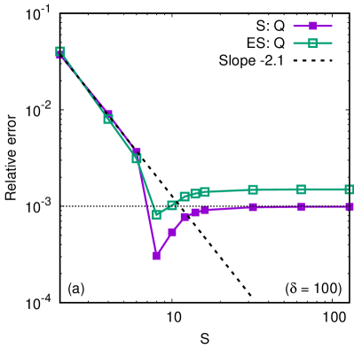
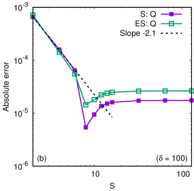
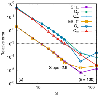
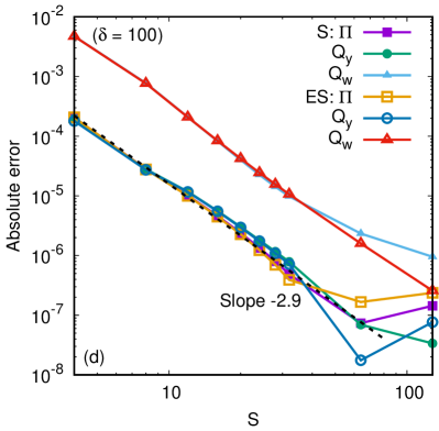
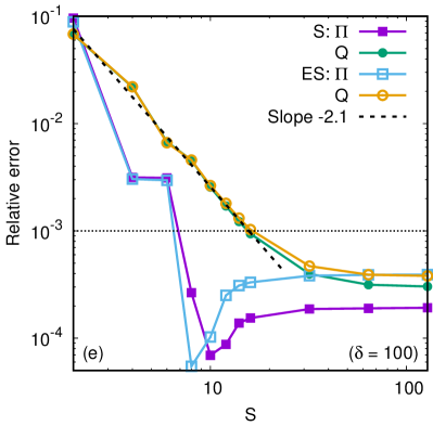
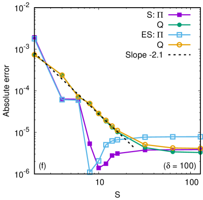
Figure 15: Convergence test for the results obtained using the projection method with respect to the number $S$ of nodes in the half channel. The heat transfer between stationary plates (top line), Couette flow (middle line) and heat transfer between moving plates (bottom line) are considered at $\delta=100$. The results obtained using the S model are shown using filled symbols, while the ES model results are represented using empty symbols. The relative (left) and absolute (right) errors are computed at the level of the various quantities introduced in Sec. 4 by taking the results obtained using the hybrid method with $Q_{x}^{\phi}=Q_{x}^{\chi}=16$ and $S=128$ as a reference. The slope of the dotted line indicates the convergence order.

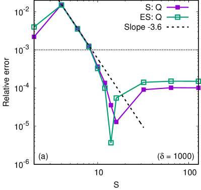
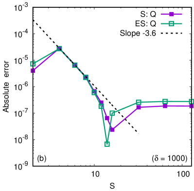
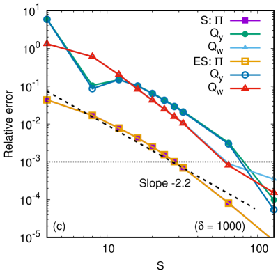
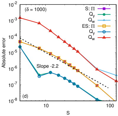
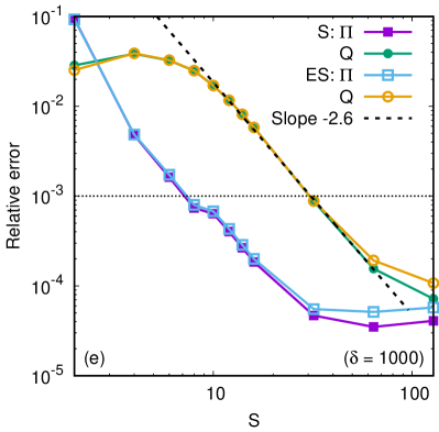
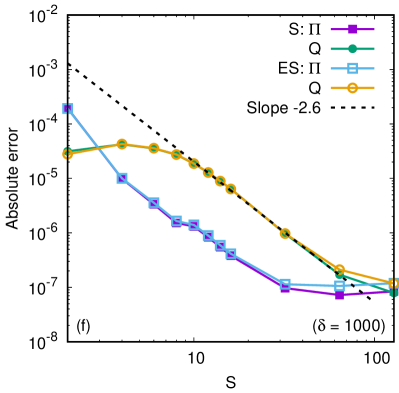
Figure 16: Same as Fig. 15, for $\delta=1000$.

	HT		SH		HT-SH
$\delta$	$T_{\rm S}({\rm s})$	$T_{\rm ES}({\rm s})$	$T_{\rm S}({\rm s})$	$T_{\rm ES}({\rm s})$	$T_{\rm S}({\rm s})$	$T_{\rm ES}({\rm s})$
$1000$	$674$	$320$	$992$	$699$	$2106$	$1368$
$100$	$67$	$32$	$108$	$68$	$197$	$135$

Table 3: Computational times (in seconds) required to reach the steady state using the projection method described in A at $\delta=100$ and $\delta=1000$, in the context of the heat transfer between stationary plates (HT), Couette flow (SH) and heat transfer under shear (HT-SH) problems, considered in Sections 5, 6 and 7.

In order to demonstrate the capabilities of the model introduced in the previous subsections, we performed simulations in the context of the problems introduced in Sections 5, 6 and 7 for $\delta=100$ and $1000$. For definiteness, we considered the ${}^{4}{\rm He}$ gas at $\widetilde{T}_{\rm ref}=300\ {\rm K}$. The simulations were performed using the quadrature orders $Q_{x}^{\phi}=5$ and $Q_{x}^{\chi}=3$ for the half-range Gauss-Hermite quadrature employed on the $p_{x}$ axis. In the case of the heat transfer between stationary plates (discussed in Sec. 5), there are no other non-trivial degrees of freedom and the total number of distinct populations is $2(Q_{x}^{\phi}+Q_{x}^{\chi})=16$. In the Couette flow and heat transfer between moving plates problems, discussed in Sections 6 and 7, the $p_{y}$ axis was discretised using the full-range Gauss-Hermite quadrature of orders $Q_{y}^{\phi}=4$ and $Q_{y}^{\chi}=2$, as discussed in Sec. 3.2. The total number of distinct population in this case is $2(Q_{x}^{\phi}Q_{y}^{\phi}+Q_{x}^{\chi}Q_{y}^{\chi})=52$. In the context of this subsection, we refer to the method employing the models described above as the “projection method.”

In order to validate the results obtained with the projection method, we also performed simulations using the hybrid models introduced in Sec. 3, which differ from the former since the equilibrium distributions are replaced by truncated expansions only with respect to the $p_{y}$ axis. The quadrature orders in the hybrid approach are set to $Q_{x}^{\phi}=Q_{x}^{\chi}=16$, while the quadrature orders $Q_{y}^{\phi}$ and $Q_{y}^{\chi}$ remain unchanged with respect to those employed within the projection method.

Figures 15 and 16 show convergence tests performed at $\delta=100$ and $1000$, respectively, comparing the results obtained using the projection method for various values of $S$ with those obtained using the hybrid method using $Q_{x}=16$ and $S=128$, in the context of the heat transfer between stationary plates (top line), Couette flow (middle line) and heat transfer between moving plates (bottom line) problems. The left columns of Figs. 15 and 16 show the relative errors, while the right columns show the corresponding absolute errors, computed at the level of the $Q$, $\Pi$, $Q_{y}$ and $Q_{w}$ quantities introduced in Sec. 4. The resulting convergence orders take values between $2.1$ and $3.6$, depending on $\delta$ and on the quantity being analysed.

While the relative errors in $Q$ and $\Pi$ quickly approach $0.1\%$ as $S$ is increased, it can be seen from the left columns of Figs. 15 and 16 that achieving the same level of relative error for $Q_{w}$ and $Q_{y}$ in the context of the Couette flow becomes more challenging at large $\delta$. Taking into account that all quantities decrease in absolute value as $\delta^{-1}$ (except $Q_{y}$, which decreases as $\delta^{-2}$), the relative error is correspondingly amplified and thus becomes less relevant. By comparison, the right columns of the same figures show that the absolute errors are several orders of magnitude below the relative errors. It can be seen that reasonable results are obtained using the projection method with $S=32$, which gives absolute errors that are below $10^{-4}$ for al quantities under consideration. The corresponding runtimes for $S=32$ are summarised in Table 3.

References

- [1] C. Cercignani. Rarefied Gas Dynamics: From Basic Concepts to Actual Calculations. Cambridge University Press, Cambridge, 2000.
- [2] Y. Sone. Molecular Gas Dynamics: Theory, Techniques and Applications. Birkhäuser, Boston, 2007.
- [3] S. Takata and H. Funagane. Singular behaviour of a rarefied gas on a planar boundary. J. Fluid Mech., 717:30–47, 2013.
- [4] M. Gad-el-Haq. MEMS Handbook. CRC Press, Boca Raton, 2006.
- [5] G. A. Bird. Molecular Gas Dynamics and the Direct Simulation of Gas Flows. Oxford University Press, Oxford, 1994.
- [6] F. Sharipov and J. L. Strapasson. Benchmark problems for mixtures of rarefied gases. I. Couette flow. Phys. Fluids, 25:027101, 2013.
- [7] F. Sharipov and J. L. Strapasson. Ab initio simulation of rarefied gas flow through a thin orifice. Vacuum, 109:246–252, 2014.
- [8] F. Sharipov and C. F. Dias. Ab initio simulation of planar shock waves. Computers and Fluids, 150:115–122, 2017.
- [9] A. N. Volkov and F. Sharipov. Flow of a monatomic rarefied gas over a circular cylinder: Calculations based on the ab initio potential method. Int. J. Heat Mass Transfer., 114:47–61, 2017.
- [10] L. Zhu, L. Wu, Y. Zhang, and F. Sharipov. Ab initio calculation of rarefied flows of helium-neon mixture: Classical vs quantum scatterings. Int. J. Heat Mass Tran., 145:118765, 2019.
- [11] F. Sharipov. Modeling of transport phenomena in gases based on quantum scattering. Physica A, 508:797–805, 2018.
- [12] F. Sharipov and C. F. Dias. Temperature dependence of shock wave structure in helium and neon. Phys. Fluids, 31:037109, 2019.
- [13] C. Mouhot and L. Pareschi. Fast algorithms for computing the Boltzmann collision operator. Math. Comput., 75:1833–1852, 2006.
- [14] F. Filbet. On deterministic approximation of the Boltzmann equation in a bounded domain. Multiscale Model. Simul., 10:792–817, 2012.
- [15] L. Wu, C. White, T. J. Scanlon, J. M. Reese, and Y. Zhang. Deterministic numerical solutions of the Boltzmann equation using the fast spectral method. J. Comput. Phys., 250:27–52, 2013.
- [16] L. Wu, H. Liu, Y. Zhang, and J. M. Reese Influence of intermolecular potentials on rarefied gas flows: Fast spectral solutions of the Boltzmann equation. Phys. Fluids, 27:082002, 2015.
- [17] I. M. Gamba, J. R. Haack, C. D. Hauck, and J. Hu. A fast spectral method for the Boltzmann collision operator with general collision kernels. SIAM J. Sci. Comput., 39:B658–B674, 2017.
- [18] P. L. Bhatnagar, E. P. Gross, and M. Krook. A model for collision processes in gases. I. Small amplitude processes in charged and neutral one-component systems. Phys. Rev., 94:511–525, 1954.
- [19] L. H. Holway, Jr. New statistical models for kinetic theory: methods of construction. Phys. Fluids, 9:1658–1673, 1966.
- [20] E. M. Shakhov. Generalization of the Krook kinetic relaxation equation. Fluid Dyn., 3:95–96, 1968.
- [21] E. M. Shakhov. Approximate kinetic equations in rarefied gas theory. Fluid Dyn., 3:112–115, 1968.
- [22] F. Sharipov. Application of the Cercignani-Lampis scattering kernel to calculations of rarefied gas flows. I. Plane flow between two parallel plates. Eur. J. Mech. B-Fluid, 21:113–123, 2002.
- [23] F. Sharipov. Application of the Cercignani-Lampis scattering kernel to calculations of rarefied gas flows. II. Slip and jump coefficients. Eur. J. Mech. B-Fluid, 22:133–143, 2003.
- [24] I. A. Graur and A. P. Polikarpov. Comparison of different kinetic models for the heat transfer problem. Heat Mass Transfer, 46:237–244, 2009.
- [25] V. E. Ambru\cbs and V. Sofonea. High-order thermal lattice Boltzmann models derived by means of Gauss quadrature in the spherical coordinate system. Phys. Rev. E, 86:016708, 2012.
- [26] J. P. Meng, Y. H. Zhang, N. G. Hadjiconstantinou, G. A. Radtke, and X. W. Shan. Lattice ellipsoidal statistical BGK model for thermal non-equilibrium flows. J. Fluid. Mech., 718:347–370, 2013.
- [27] V. E. Ambru\cbs and V. Sofonea. Half-range lattice Boltzmann models for the simulation of Couette flow using the Shakhov collision term. Phys. Rev. E, 98:063311, 2018.
- [28] J. E. Broadwell. Study of rarefied shear flow by the discrete velocity method. J. Fluid Mech., 19:401–414, 1964.
- [29] F. Sharipov. Rarefied gas dynamics: Fundamentals for research and practice. Wiley-VCH, Weinheim, 2016.
- [30] M. T. Ho and I. Graur. Heat transfer through rarefied gas confined between two concentric spheres. Int. J. Heat Mass Transfer, 90:58–71, 2015.
- [31] Z. Guo, K. Xu, and R. Wang. Discrete unified gas kinetic scheme for all Knudsen number flows: Low-speed isothermal case. Phys. Rev. E, 88:033305, 9 2013.
- [32] Z. Guo, R. Wang, and K. Xu. Discrete unified gas kinetic scheme for all Knudsen number flows. II. thermal compressible case. Phys. Rev. E, 91:033313, 3 2015.
- [33] L. Zhu, P. Wang, and Z. Guo. Performance evaluation of the general characteristics based off-lattice Boltzmann scheme and DUGKS for low speed continuum flows. J. Comput. Phys., 333:227–246, 2017.
- [34] X. He, X. Shan, and G. D. Doolen. Discrete Boltzmann equation model for nonideal gases. Phys. Rev. E, 57:R13–R16, 1998.
- [35] C. Lin, K. H. Luo, L. Fei, and S. Succi. A multi-component discrete Boltzmann model for nonequilibrium reactive flows. Sci. Rep., 7:14580, 2017.
- [36] Y.-D. Zhang, A.-G. Xu, G.-C. Zhang, Z.-H. Chen, and P. Wang. Discrete ellipsoidal statistical BGK model and Burnett equations. Front. Phys., 13:135101, 2018.
- [37] W. P. Yudistiawan, S. Ansumali, and I. V. Karlin. Hydrodynamics beyond Navier-Stokes: The slip flow model. Phys. Rev. E, 78:016705, 2008.
- [38] W. P. Yudistiawan, S. K. Kwak, D. V. Patil, and S. Ansumali. Higher-order Galilean-invariant lattice Boltzmann model for microflows: Single-component gas. Phys. Rev. E, 82:046701, 2010.
- [39] C. Feuchter and W. Schleifenbaum. High-order lattice Boltzmann models for wall-bounded flows at finite Knudsen numbers. Phys. Rev. E, 94:013304, 2016.
- [40] M. Atif, M. Namburi, and S. Ansumali. Higher-order lattice Boltzmann model for thermohydrodynamics. Phys. Rev. E, 98:053311, 2018.
- [41] C. K. Aidun and J. R. Clausen. Lattice-Boltzmann method for complex flows. Annu. Rev. Fluid Mech., 42:439–472, 2010.
- [42] J. P. Meng and Y. H. Zhang. Gauss-Hermite quadratures and accuracy of lattice Boltzmann models for nonequilibrium gas flows. Phys. Rev. E, 83:036704, 2011.
- [43] Y. Shi, Y. W. Yap, and J. E. Sader. Linearized lattice Boltzmann method for micro- and nanoscale flow and heat transfer. Phys. Rev. E, 92:013307, 2015.
- [44] V. E. Ambru\cbs and V. Sofonea. Lattice Boltzmann models based on half-range Gauss-Hermite quadratures. J. Comput. Phys., 316:760–788, 2016.
- [45] S. Succi. The Lattice Boltzmann Equation for Fluid Dynamics and Beyond. Clarendon Press, Oxford, 2001.
- [46] P. Fede, V. Sofonea, R. Fournier, S. Blanco, O. Simonin, G. Lepoutère, and V. E. Ambru\cbs. Lattice Boltzmann model for predicting the deposition of inertial particles transported by a turbulent flow. Int. J. Multiph. Flow, 76:187–197, 2015.
- [47] T. Krüger, H. Kusumaatmaja, A. Kuzmin, O. Shardt, G. Silva, and E. M. Viggen. Lattice Boltzmann Method: Principles and Practice. Springer, 2017.
- [48] S. Succi. The Lattice Boltzmann Equation: For Complex States of Flowing Matter. Oxford University Press, 2018.
- [49] X. W. Shan, X. F. Yuan, and H. D. Chen. Kinetic theory representation of hydrodynamics: a way beyond the Navier-Stokes equation. J. Fluid. Mech., 550:413–441, 2006.
- [50] F. B. Hildebrand. Introduction to Numerical Analysis. Dover Publications, second edition edition, 1987.
- [51] B. Shizgal. Spectral Methods in Chemistry and Physics: Applications to Kinetic Theory and Quantum Mechanics (Scientific Computation). Springer, 2015.
- [52] F. Sharipov. Rarefied gas flow through a long tube at any temperature ratio. J. Vac. Sci. Technol. A, 14:2627–2635, 1996.
- [53] L. Wu, J. M. Reese, and Y. Zhang. Solving the Boltzmann equation deterministically by the fast spectral method: application to gas microflows. J. Fluid Mech., 746:53–84, 2014.
- [54] F. Sharipov. Rarefied gas flow through a long rectangular channel. J. Vac. Sci. Technol. A, 17:3062–3066, 1999.
- [55] E. P. Gross, E. A. Jackson, and S. Ziering. Boundary value problems in kinetic theory of gases. Ann. Phys., 1:141–167, 1957.
- [56] Y. Sone. Kinetic theory analysis of linearized Rayleigh problem. J. Phys. Soc. Jpn., 19:1463–1473, 1964.
- [57] S. Jiang and L.-S. Luo. Analysis and accurate numerical solutions of the integral equation derived from the linearized BGKW equation for the steady Couette flow. J. Comput. Phys, 316:416–434, 2016.
- [58] E. P. Gross and S. Ziering. Kinetic theory of linear shear flow. Phys. Fluids, 1:215–224, 1958.
- [59] S. Ziering. Shear and heat flow for Maxwellian molecules. Phys. Fluids, 3:503–509, 1960.
- [60] P. L. Bhatnagar and M. P. Srivastava. Heat transfer in plane Couette flow of a rarefied gas using Bhatnagar-Gross-Krook model. Phys. Fluids, 12:938–940, 1969.
- [61] A. Frezzotti, L. Gibelli, and B. Franzelli. A moment method for low speed microflows. Continuum Mech. Thermodyn., 21:495–509, 2009.
- [62] L. Gibelli. Velocity slip coefficients based on the hard-sphere Boltzmann equation. Phys. Fluids, 24:022001, 2012.
- [63] G. P. Ghiroldi and L. Gibelli. A direct method for the Boltzmann equation based on a pseudo-spectral velocity space discretization. J. Comput. Phys., 258:568–584, 2014.
- [64] A. B. Huang and D. P. Giddens. A new table for a modified (half range) Gauss‐Hermite quadrature with an evaluation of the integral . J. Math. Phys., 47:213–218, 1968.
- [65] J. S. Ball. Half-range generalized Hermite polynomials and the related Gaussian quadratures. SIAM J. Numer. Anal., 40:2311–2317, 2003.
- [66] Z.-H. Li and H.-X. Zhang. Numerical investigation from rarefied flow to continuum by solving the Boltzmann model equation. Int. J. Numer. Meth. Fluids, 42:361–382, 2003.
- [67] Z.-H. Li and H.-X. Zhang. Study on gas kinetic unified algorithm for flows from rarefied transition to continuum. J. Comput. Phys, 193:708–738, 2004.
- [68] G. P. Ghiroldi and L. Gibelli. A finite-difference lattice Boltzmann approach for gas microflows. Commun. Comput. Phys., 17:1007–1018, 2015.
- [69] V. E. Ambru\cbs and V. Sofonea. Lattice Boltzmann models based on Gauss quadratures. Int. J. Mod. Phys. C, 25:1441011, 2014.
- [70] V. E. Ambru\cbs and V. Sofonea. Implementation of diffuse-reflection boundary conditions using lattice Boltzmann models based on half-space Gauss-Laguerre quadratures. Phys. Rev. E, 89:041301(R), 4 2014.
- [71] V. E. Ambru\cbs and V. Sofonea. Quadrature-based lattice Boltzmann models for rarefied gas flow. In: F. Toschi and M. Sega, editors, Flowing Matter. Soft and Biological Matter, chapter 9, 271–299. Springer, Cham, 2019.
- [72] D. Valougeorgis and S. Naris. Acceleration schemes of the discrete velocity method: Gaseous flows in rectangular microchannels. SIAM J. Sci. Comput., 25:534–552, 2003.
- [73] L. Wu, J. Zhang, H. Liu, Y. Zhang, and J. M. Reese. A fast iterative scheme for the linearized Boltzmann equation. J. Comput. Phys., 338:431–451, 2017.
- [74] W. Su, P. Wang, H. Liu, and L. Wu. Accurate and efficient computation of the Boltzmann equation for Couette flow: Influence of intermolecular potentials on Knudsen layer function and viscous slip coefficient. J. Comput. Phys., 378:573–590, 2019.
- [75] L. Zhu, X. Pi, W. Su, Z.-H. Li, Y. Zhang, and L. Wu. General Synthetic Iteration Scheme for Non-linear Gas Kinetic Simulation of Multi-scale Rarefied Gas flows. arXiv:2004.10530 [physics.comp-ph].
- [76] Chi-Wang Shu and Stanley Osher. Efficient implementation of essentially non-oscillatory shock-capturing schemes. J. Comput. Phys., 77:439–471, 1988.
- [77] S. Gottlieb and C.-W. Shu. Total variation diminishing Runge-Kutta schemes. Math. Comput., 67:73–85, 1998.
- [78] J. A. Trangenstein. Numerical solution of hyperbolic partial differential equations. Cambridge University Press, New York, 2007.
- [79] V. E. Ambru\cbs and L.-S. Luo. Analysis of Knudsen layer phenomena using half-range quadratures. 2019. In preparation.
- [80] R. Mei and W. Shyy. On the finite difference-based lattice Boltzmann method in curvilinear coordinates. J. Comput. Phys., 143:426–448, 1998.
- [81] Z. Guo and T. S. Zhao. Explicit finite-difference lattice Boltzmann method for curvilinear coordinates. Phys. Rev. E, 67:066709, 2003.
- [82] S. Busuioc and V. E. Ambru\cbs. Lattice Boltzmann models based on the vielbein formalism for the simulation of flows in curvilinear geometries. Phys. Rev. E, 99:033304, 2019.
- [83] V. Sofonea and R. F. Sekerka. Viscosity of finite difference lattice Boltzmann models. J. Comput. Phys., 183:422–434, 2003.
- [84] V. Sofonea, A. Lamura, G. Gonnella, and A. Cristea. Finite-difference lattice Boltzmann model with flux limiters for liquid-vapor systems. Phys. Rev. E, 70:046702, 2004.
- [85] S. Naris, D. Valougeorgis, D. Kalempa, and F. Sharipov. Gaseous mixture flow between two parallel plates in the whole range of the gas rarefaction. Physica A, 336:294–318, 2004.
- [86] C. Tantos and D. Valougeorgis. Conductive heat transfer in rarefied binary gas mixtures confined between parallel plates based on kinetic modeling. Int. J. Heat Mass Tran., 117:846–860, 2018.
- [87] C. Cercignani and M. Lampis. Kinetic model for gas-surface interaction. Transp. Theory Stat. Phys., 1:101–114, 1971.
- [88] V. E. Ambru\cbs, F. Sharipov, and V. Sofonea. Lattice Boltzmann approach to rarefied gas flows using half-range Gauss-Hermite quadratures: Comparison to DSMC results based on ab initio potentials. AIP Conf. Proc., 2132:060012, 2019.
- [89] J. Meng, L. Wu, J. M. Reese, and Y. Zhang. Assessment of the ellipsoidal-statistical Bhatnagar-Gross-Krook model for force-driven Poiseuille flow. J. Comput. Phys., 251:383–395, 2013.
- [90] W. Cencek, M. Przybytek, J. Komasa, J. B. Mehl, B. Jeziorski, and K. Szalewicz. Effects of adiabatic, relativistic and quantum electrodynamics interactions on the pair potential and thermophysical properties of helium. J. Chem. Phys., 136:224303, 2012.
- [91] F. Sharipov and V. J. Benites. Transport coefficients of helium-neon mixtures at low density computed from ab initio potentials. J. Chem. Phys., 147:224302, 2017.
- [92] V. E. Ambru\cbs and V. Sofonea. Application of mixed quadrature lattice Boltzmann models for the simulation of Poiseuille flow at non-negligible values of the Knudsen number. J. Comput. Sci., 17:403–417, 2016.
- [93] S. Ansumali, I. V. Karlin, and H. C. Öttinger. Minimal entropic kinetic models for hydrodynamics. Europhys. Lett., 63:798, 2003.
- [94] A. Bardow, I. V. Karlin, and A. A. Gusev. General characteristic-based algorithm for off-lattice Boltzmann simulations. Europhys. Lett., 75:434, 2006.
- [95] A. Bardow, I. V. Karlin, and A. A. Gusev. Multispeed models in off-lattice Boltzmann simulations. Phys. Rev. E, 77:025701(R), 2008.
- [96] T. Biciu\cbscă, A. Horga, and V. Sofonea. Simulation of liquid-vapour phase separation on GPUs using Lattice Boltzmann models with off-lattice velocity sets. C. R. Mecanique, 343:580–588, 2015.
- [97] V. Sofonea, T. Biciu\cbscă, S. Busuioc, V. E. Ambru\cbs, G. Gonnella, and A. Lamura. Corner-transport-upwind lattice Boltzmann model for bubble cavitation. Phys. Rev. E, 97:023309, 2018.
- [98] L. Pareschi and G. Russo. Implicit-Explicit Runge-Kutta schemes and applications to hyperbolic systems with relaxation. J. Sci. Comput., 25:129–155, 2005.
- [99] Y. Wand, Y. L. He, T. S. Zhao, G. H. Tang, and W. Q. Tao. Implicit-Explicit finite-difference lattice Boltzmann method for compressible flows. Int. J. Mod. Phys. C, 18:1961–1983, 2007.
- [100] S. T. Kis and V. E. Ambru\cbs. Implicit-explicit finite-difference lattice Boltzmann model with varying adiabatic index. AIP Conf. Proc., 2218:050008, 2020.
- [101] Jr. W. Marques, G. M. Kremer, and F. M. Sharipov. Couette flow with slip and jump boundary conditions. Continuum Mech. Thermodyn., 12:379–386, 2000.
- [102] Satish Balay, Shrirang Abhyankar, Mark F. Adams, Jed Brown, Peter Brune, Kris Buschelman, Lisandro Dalcin, Victor Eijkhout, William D. Gropp, Dinesh Kaushik, Matthew G. Knepley, Lois Curfman McInnes, Karl Rupp, Barry F. Smith, Stefano Zampini, and Hong Zhang. PETSc users manual. Technical Report ANL-95/11 - Revision 3.6, Argonne National Laboratory, 2015.
- [103] Satish Balay, William D. Gropp, Lois Curfman McInnes, and Barry F. Smith. Efficient management of parallelism in object oriented numerical software libraries. In E. Arge, A. M. Bruaset, and H. P. Langtangen, editors, Modern Software Tools in Scientific Computing, pages 163–202. Birkhäuser Press, 1997.
- [104] P. K. Kundu, I. M. Cohen, D. R. Dowling, Fluid Mechanics, 6th Ed. (Academic Press, 2016).