Learning A Unified Named Entity Tagger From Multiple Partially Annotated Corpora For Efficient Adaptation

Abstract

Named entity recognition (NER) identifies typed entity mentions in raw text. While the task is well-established, there is no universally used tagset: often, datasets are annotated for use in downstream applications and accordingly only cover a small set of entity types relevant to a particular task. For instance, in the biomedical domain, one corpus might annotate genes, another chemicals, and another diseases—despite the texts in each corpus containing references to all three types of entities. In this paper, we propose a deep structured model to integrate these “partially annotated” datasets to jointly identify all entity types appearing in the training corpora. By leveraging multiple datasets, the model can learn robust input representations; by building a joint structured model, it avoids potential conflicts caused by combining several models’ predictions at test time. Experiments show that the proposed model significantly outperforms strong multi-task learning baselines when training on multiple, partially annotated datasets and testing on datasets that contain tags from more than one of the training corpora.

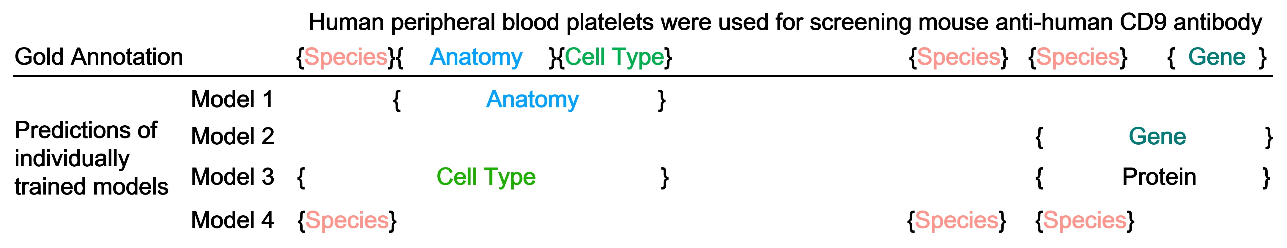
Figure 1: An example sentence from the CellFinder corpus Neves et al. (2012) showing the challenges in combining the output of individual NE taggers. The Gold row is the human annotations in CellFinder. The rows below are predictions made by models trained on datasets that each contain only a subset of the CellFinder types. Note that the individual taggers’ predictions can conflict with each other, making it challenging to combine them. (Note: we renamed CellFinder’s Cell Component to Cell Type to fit it in the space above.)

1 Introduction

Named Entity Recognition (NER), which identifies the boundaries and types of entity mentions from raw text, is a fundamental problem in natural language processing (NLP). It is a basic component for many downstream tasks, such as relation extraction Hasegawa et al. (2004); Mooney and Bunescu (2005), coreference resolution Soon et al. (2001), and knowledge base construction Craven et al. (1998); Craven and Kumlien (1999).

One problem in NER is the diversity of entity types, which vary in scope for different domains and downstream tasks. Traditional NER for the news domain focuses on three coarse-grained entity types: person, location, and organization Tjong Kim Sang and De Meulder (2003). However, as NLP technologies have been applied to a broader set of domains, many other entity types have been targeted. For instance, Ritter et al. (2011) add seven new entity types (e.g., product, tv-show) on top of the previous three when annotating tweets. Other efforts also define different but partially overlapping sets of entity types Walker et al. (2006); Ji et al. (2010); Consortium (2013); Aguilar et al. (2014). These non-unified annotation schemas result in partially annotated datasets: each dataset is only annotated with a subset of possible entity types.

One approach to this problem is to train individual NE taggers for each partially annotated dataset and combine their results using some heuristics. Figure 1 shows an example that demonstrates the possible shortcomings of this approach, using the biomedical domain as a case study. Here, we train four separate models on four partially annotated datasets: AnatEM Pyysalo and Ananiadou (2013) annotated for the anatomy type, BC2GM Smith et al. (2008) for the gene type, JNLPBA Kim et al. (2004) for cell types, and Linnaeus Gerner et al. (2010) for the species type. We can see that the models’ predictions contradict each other when applied to the same test sentence—making it a challenge to accurately combine them.

In this paper, we propose a deep structured model to leverage multiple partially annotated datasets, allowing us to jointly identify the union of all entity types presented in the training data. The model leverages supervision signals across diverse datasets to learn robust input representations, thus improving the performance for each entity type. Moreover, it makes joint predictions to avoid potential conflicts among models built on different entity types, allowing further improvement for cross-type NER.

Experiments on both real-world and synthetic datasets show that our model can efficiently adapt to new corpora that have more types than any individual dataset used for training and that it achieves significantly better results compared to strong multi-task learning baselines.

2 Problem Statement

We formally define the problem by first defining our terminology.

Global Tag Space. Let $C_{i}$ denote a corpus, and $T_{C_{i}}$ denote the set of entity types that are tagged in corpus $C_{i}$. When there are a set of corpora $\mathbb{C}=\{C_{1},C_{2},...,C_{n}\}$, each has its own tag space concerning different entity types, the global tag space is defined as the union of the local tag space. Formally, $T_{\mathbb{C}}=T_{C_{1}}\cup T_{C_{2}}\cup...\cup T_{C_{n}}$.

Partially Annotated Corpus. If $T_{C_{i}}\subsetneqq T_{\mathbb{C}}$, then $C_{i}$ is a partially annotated corpus.

Global Evaluation. When a model is trained on a set of partially annotated corpora $\mathbb{C}$ and predicts tags for the whole global tag space $T_{\mathbb{C}}$, we say it is making global predictions. Accordingly, the evaluation of the models’ performance on $T_{\mathbb{C}}$ is called global evaluation.

Our goal is to train a single unified NE tagger from several partially annotated corpora for efficient adaptation to new corpora that have more types than any individual dataset used during training. Formally, we have a set of corpora $\mathbb{C}=\{C_{1},C_{2},...,C_{n}\}$, and we propose to train a joint model on $\mathbb{C}$ such that it makes predictions for the global tag space $T_{\mathbb{C}}$. One benefit of this joint model is that it can be easily adapted to a new tag space $T_{C_{u}}$ where $T_{C_{u}}\subseteq T_{\mathbb{C}}$, and $T_{C_{u}}\nsubseteq T_{C_{i}},\forall C_{i}\in\mathbb{C}$.

3 Background and Related Work

In this section, we first introduce neural architectures for NER which our work builds upon and then summarize previous work on imperfect annotation problems.

3.1 Neural Architectures for NER

With recent advances using deep neural networks, bi-directional long short-term memory networks with conditional random fields (BiLSTM-CRF) have become standard for NER Lample et al. (2016). A typical architecture consists of a BiLSTM layer to learn feature representations from the input and a CRF layer to model the inter-dependencies between adjacent labels and perform joint inference. Ma and Hovy (2016) introduce additional character-level convolutional neural networks (CNNs) to capture subword unit information. In this paper, we use a BiLSTM-CRF with character-level modeling as our base model. We now briefly review the BiLSTM-CRF model.

BiLSTMs.

Long Short Term Memory networks (LSTMs) Hochreiter and Schmidhuber (1997) are a variation of RNNs that are designed to avoid the vanishing/exploding gradient problem Bengio et al. (1994). Specifically, BiLSTMs take as input a sequence of words $\bm{x}=\{x_{k}|k\in\mathcal{N}\}$ and output a sequence of hidden vectors: $\bm{H}=\{h_{k}|k\in\mathcal{N}\}$ BiLSTMs combine a left-to-right (forward) and a right-to-left (backward) LSTM to capture both left and right context. Formally, they produce a hidden vector $\tilde{\bm{h}}_{i}=[\overrightarrow{\bm{h}_{i}};\overleftarrow{\bm{h}_{i}}]$ for each input, where $\overrightarrow{\bm{h}_{i}}$ and $\overleftarrow{\bm{h}_{i}}$ are produced by the forward and the backward LSTMs respectively; $[;]$ denotes vector concatenation.

Character-level Modeling.

Following Wang et al. (2018), we use a BiLSTM for character-level modeling. We concatenate the hidden vector of the space after a word from the forward LSTM and the hidden vector of the space before a word from the backward LSTM to form a character-level representation of the word: $\bm{h}^{c}_{i}=[\overrightarrow{\bm{h}_{i}^{c}};\overleftarrow{\bm{h}^{c}_{i}}]$. The word-level BiLSTM then takes the concatenation of $\bm{h}^{c}_{i}$ and the word embedding as input $\bm{x}_{i}=[\bm{e}_{i};\bm{h}^{c}_{i}]$ to learn contextualized representations.

Neural-CRFs.

Conditional Random Fields (CRFs) Lafferty et al. (2001) are sequence tagging models that capture the inter-dependencies between the output tags; they have been widely used for NER McCallum and Li (2003); Lu et al. (2015); Peng and Dredze (2015, 2016, 2017). Given a set of training data $\{\bm{x}_{i},\bm{y}_{i}\}^{N}$, a CRF minimizes negative log-likelihood:

$$\min_{\Theta}-\sum_{i}\log P(\bm{y}_{i}\mid\bm{x}_{i};\Theta),$$ (1)

$$P(\bm{y}_{i}\mid\bm{x}_{i};\Theta)=\frac{Gold\,Energy}{Partition}=\frac{St(\bm{y}_{i})}{\sum_{\bm{y}^{\prime}}St(\bm{y}^{\prime})}$$ (2)

where $\bm{y}^{\prime}$ is any possible tag sequence with the same length as $\bm{y}_{i}$, $St(\bm{y}^{\prime})$ is the potential of the tag sequence $\bm{y}^{\prime}$, and $St(\bm{y}_{i})$ is the potential of the gold tag sequence. The numerator $St(\bm{y}_{i})$ is called the gold energy function, and the denominator $\sum_{\bm{y}^{\prime}}St(\bm{y}^{\prime})$ is the partition function. The likelihood function using globally annotated data is illustrated in Figure 2(a). The potential of a tag sequence can be computed as:

$$St(\bm{y})=\prod_{t=1}^{|\bm{y}|}Score(\bm{y}[t],\bm{y}[t-1])$$ (3)

where $\bm{y}[t]$ is the $t$th element in $\bm{y}$ ($\bm{y}[-1]$ is the start of the sequence), and

$$\begin{split}Score(\bm{y}[t],\bm{y}[t-1])=&\exp\left(tr(\bm{y}[t],\bm{y}[t-1])\right)*\\ &\exp\left(em(\bm{y}[t])\right)\end{split}$$ (4)

where $tr(\bm{y}[t],\bm{y}[t-1])$ is the transition score from $\bm{y}[t-1]$ to $\bm{y}[t]$, and $em(\bm{y}[t])$ is the emission score of $\bm{y}[t]$ computed based on the output $\tilde{\bm{h}}_{t}$ of the BiLSTM.

3.2 Learning from Imperfect Annotations

Learning from multiple partially annotated datasets could be more generally thought of as learning from imperfect annotations. In that broad sense, there are several notable areas of prior work. One of the most prominent concerns learning from incomplete annotations (noisy labels), where some occurrences of entities are neglected in the annotation process and falsely labeled as non-entities (negative). A related problem is learning from unlabeled data with distant supervision.

A major challenge of all these settings, including ours, is that a positive instance might be labeled as negative. A well-explored solution to this problem is proposed by Tsuboi et al. (2008), which instead of maximizing the likelihood of the gold tag sequence, we maximize the total likelihood for all possible tag sequences consistent with the gold labels. Tsuboi et al. (2008); Yang and Vozila (2014) applied this idea to the incomplete annotation setting; Shang et al. (2018); Liu et al. (2014) applied it to the unlabeled data with distant supervision setting; and Greenberg et al. (2018) applied it to the partial annotation setting. While this is a general solution, its primary drawback is that it assumes a uniform prior on all labels consistent with the gold labels. This may have the result of overly encouraging the prediction of entities, resulting in low precision.

To tackle the problem of incomplete annotations, Carlson et al. (2009); Yang et al. (2018) explored bootstrap-based semi-supervised learning on unlabeled data, iteratively identifying new entities with the taggers and then re-training the taggers. Bellare and McCallum (2007); Li and Liu (2005); Fernandes and Brefeld (2011) explored an EM algorithm with semi-supervision.

For the partial annotation problem, most previous work has focused on building individual taggers for each dataset and using single-task learning Liu et al. (2018) or multi-task learning Crichton et al. (2017); Wang et al. (2018). In single-task learning, each model is trained separately on each dataset $C_{i}$, and makes local predictions on $T_{C_{i}}$. Based on the neural-CRF architecture, multi-task learning uses a different CRF layer for each dataset $C_{i}$ (each task) to make local predictions on $T_{C_{i}}$, and shares the lower-level representation learning component across all tasks. Both single-task learning and multi-task learning make local predictions and have to apply heuristics to combine the model predictions, resulting in the collision problem demonstrated in Figure 1.

To the best of our knowledge, Greenberg et al. (2018) is the only prior work trying to build a unified model from multiple partially annotated corpora. We will show that their model, which is reminiscent of Tsuboi et al. (2008), is a special case of ours and that our other variations achieve better performance. In addition, they only evaluated the model on the training corpora while we conduct evaluations to test the model’s ability to adapt to new corpora with different tag spaces.

4 Model

As mentioned above, we use a BiLSTM-CRF with character-level modeling as our base model. Our goal is to build a unified model to make global predictions. That is, our model will be jointly trained on multiple partially annotated datasets $\mathbb{C}$ and make predictions on the global tag space $T_{\mathbb{C}}$. Such a unified model will enjoy the benefit of learning robust representations from multiple datasets just like multi-task learning while maintaining a joint probability distribution of the global tag space to avoid possible conflicts from individual models.

4.1 Naive Approach

A simple solution to the problem is to merge all the datasets into one giant corpus. A single model can then be trained on this corpus to make global predictions. However, such a corpus will be missing many correct annotations, since each portion will be annotated with only a subset of the target entity types. Figure 2(b) shows an example: here, a location (Texas) exists but is labeled as a non-entity, because the original dataset from which this sentence is drawn does not annotate locations at all. As a result, this approach suffers from false penalties when applying the original likelihood function (Eq. 2-4) to train the model, meaning that it penalizes predictions that correctly identify entities with types that are not annotated for a particular sentence.

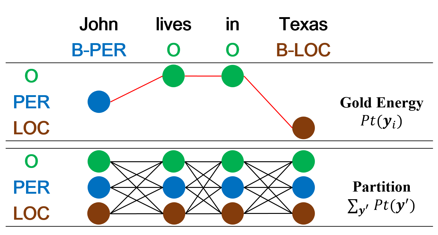
(a) Original likelihood function with global annotation

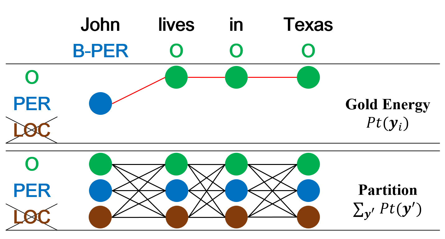
(b) Original likelihood function with partial annotation

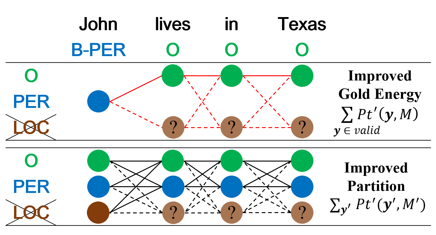
(c) Improved likelihood function with partial annotation

Figure 2: Illustration of original (2(a), 2(b)) and improved (2(c)) likelihood functions. Each figure has two parts upper and lower that illustrate the gold energy (numerator) and the partition (denominator) respectively. Solid lines represent tag sequences that are fully considered in the functions. Dashed lines represent tag sequences that are discounted. The sentences in 2(b) and 2(c) are not annotated with LOC.

4.2 Improving the Gold Energy Function

One way to improve performance is to explicitly acknowledge the incompleteness of the existing “gold” annotations and to give the model credit for predicting any tag sequence that is consistent with the partial annotations. This can be done by modifying the CRF’s gold energy function, illustrated in the upper part of Figure 2(c). Specifically, in this example, John is labeled as PER, so PER is the only possible correct tag at that position. However, lives, in, and Texas are labeled as O (non-entity), which here means only that they may not be PER—but any of them could be LOC, since locations are not annotated for this sentence. Therefore, any sequence that assigns either O or LOC for any of these three positions is consistent with the gold labels. To account for this, we modify the gold energy function to credit all tag sequences that are consistent with the gold annotations, encouraging the model to predict other consistent labels when the gold label is O. Tsuboi et al. (2008) propose a specific solution that applies this idea on incomplete annotations: instead of maximizing the likelihood of the gold tag sequence when optimizing the CRF model, they maximize the total likelihood of all possible tag sequences consistent with the gold labels. This approach is later used by Greenberg et al. (2018) to handle the problem of partial annotation. We will address a potential problem with their method and propose a generalized version in Section 4.4.

4.3 Improving the Partition Function

Modifying the gold energy function will give credit to a system for producing alternative entity labels for words tagged as O in the partially annotated training. A different solution is to simply not penalize predictions of such alternative labels. This can be done by modifying the partition function and keeping the gold energy function unchanged. The lower part of Figure 2(c) gives an illustration. As stated above, LOC is a consistent alternative entity label for lives, in, and Texas. We therefore exclude from our calculations any paths that include LOC at any of those positions. More generally, we exclude all such consistent but alternative tag sequences from the computation of the CRF’s partition function. Section 4.4 gives formal definitions with equations. The improved partition function sets the model free to predict alternative labels without penalty (as long as they are consistent with the known gold annotations), but it does not give them any positive credit for doing so (as in the previous approach). We hypothesize that the improved partition function would work better than the improved gold energy function in our setting because it addresses the false penalties problem more precisely. We will verify this hypothesis in our experiments.

4.4 Discounting Alternative Sequences

There is a potential problem with naively applying the improved gold energy function: when the gold label is O, the model is encouraged to predict other consistent labels as strongly as it is encouraged to predict O. However, many O labels are confident annotations of O. As a result, naively training with the improved gold energy function tends to over-predict entities and not predict Os. To mitigate this problem, we discount the energy of tag sequences that go through alternative labels. This can be achieved by introducing a hyper-parameter $M\text{(mask)}\in[0,1]$ as a discounting factor for the gold energy function. Formally, we modify Eq 3 to:

$$St^{\prime}(\bm{y},M)=$$

$$\prod_{t=1}^{|\bm{y}|}(Score(\bm{y}[t],\bm{y}[t-1])*mask(\bm{y}[t],M)),$$

where

$$mask(\bm{y}[t],M)=\begin{cases}M,&\text{if }\bm{y}[t]\in alternative\\ 1,&\text{Otherwise}\end{cases}.$$

where $alternative$ is the set of alternative labels. We thus have the improved gold energy function:

$$Improved\,Gold\,Energy=\sum_{\bm{y}\in valid}St^{\prime}(\bm{y},M),$$ (5)

where $valid$ is the set of all tag sequences that are consistent with the gold sequence, including the gold sequence itself.

Similarly, for the improved partition function, we can use the same strategy to discount the energy of alternative sequences rather than completely removing them. We thus introduce another $M^{\prime}\in[0,1]$ and the improved partition function becomes:

$$Improved\,Partition=\sum_{\bm{y}^{\prime}}St^{\prime}(\bm{y}^{\prime},M^{\prime}),$$ (6)

4.5 Combining Improved Functions

For generality, we combine the improved gold energy and the improved partition function to make a new likelihood function as our final model:

$$Improved\,LH=\frac{\sum_{\bm{y}\in valid}St^{\prime}(\bm{y},M)}{\sum_{\bm{y}^{\prime}}St^{\prime}(\bm{y}^{\prime},M^{\prime})}$$ (7)

To ensure Equation 7 is a valid likelihood function (the probabilities of all sequences sum to 1), we need a constraint that $M=M^{\prime}$. Note that Equation 7 subsumes all models discussed in this section. Specifically, when $M=0,M^{\prime}=1$, the model is the Naive Model discussed in Section 4.1; when $M=1,M^{\prime}=1$, the model is the same as Greenberg et al. (2018) discussed in Section 4.2; when $M=0,M^{\prime}=0$, the model is the same as proposed in Section 4.3. We have a general perspective of all the models by simply treating $M$ and $M^{\prime}$ as hyper-parameters.

Note that for the Naive Model, since $M!=M$, the Equation 7 is not always a valid likelihood function. This may partially explain why the Naive Model performs so poorly under this setting. We posit that the model will work the best when $M=M^{\prime}$.

5 Experimental Setup

5.1 Datasets

Our goal is to train a unified NER model on multiple partially annotated datasets. This model will make global predictions and can efficiently adapt to new corpora that contain tags from more than one training corpus. To fully test this capability, we would need a single test set annotated with all types of interest. However, the motivation behind this effort is that such a dataset typically does not exist. We therefore take two approaches to approximate such an evaluation.

In the first evaluation setting, we take advantage of the fact that although there may not be a single dataset annotated with all types of named entities of interest, there exist several datasets that cover types from more than one of the training corpora. Specifically, we are able to select test corpora that each cover types of interest from multiple training corpora. Table 1 shows the biomedical corpora we use and their entity types. For example, we use BC5CDR for global evaluation, because its entity types (Chemical and Disease) cover multiple training corpora (BC4CHEM for Chemical and NCBI for Disease).

For Training
Corpus	Entities
BC2GM	GP
BC4CHEM	Chemical
NCBI	Disease
JNLPBA	GP, DNA, Cell-type, Cell-line, RNA
Linnaeus	Species

For Global Evaluations
Corpus	Entities
BC5CDR	Chemical, Disease
BioNLP13CG	GP, Disease, Chemical, others
BioNLP11ID	GP, Chemical, others

Table 1: Details of the biomedical corpora. “others” denotes NE types that do not appear in the training corpora, and thus are not evaluated.

In the second evaluation setting, we create synthetic datasets from the CoNLL 2003 NER dataset to simulate training and global evaluations. Specifically, the CoNLL 2003 dataset is annotated with four entity types: location, person, organization, and miscellaneous entities. We randomly split the training set into four portions, each containing only one entity type (all other types are removed). In this setting, the four portions of the training set are used for training and the original dataset with all entities annotated is used as a global corpus.

More details about all the datasets can be found in Appendix A.1.

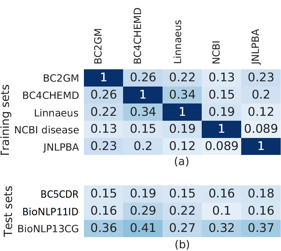
Figure 3: (a) The mention-level overlap among training sets. (b) The mention-level overlap between training datasets and evaluation datasets.

5.1.1 Biomedical Dataset Analysis

The motivation for this work rests on the assumption that even when a dataset is annotated for a certain set of entity types, it likely contains other types of entities that are unlabeled. To verify this assumption, we expand the annotations of each dataset using heuristics and compute the pairwise mention-level overlap between the datasets. Specifically, suppose we are comparing two datasets, A and B. We first construct A’ and B’, where A’ contains all mentions in A but is augmented with new mentions found by taking all strings annotated in B and marking them as named entities in A (regardless of context; there may obviously be some errors). We do the same (in the opposite direction) to construct B’. We then compute the pairwise overlap coefficient between A’ and B’ according to the following criterion:

$$\mathrm{overlap}(A^{\prime},B^{\prime})={\frac{|A^{\prime}\cap B^{\prime}|}{\min(|A^{\prime}|,|B^{\prime}|)}}.$$

Figure 3 shows the heat maps. For the training group, BC2GM, BC4CHEMD, and Linnaeus are considerably overlapped, although they are annotated with different entity types (GP, Chemical, and Species). This confirms our assumption that although the datasets are annotated for a subset of entity types, they contain other types that are unlabeled.

Corpus	Trained on Other Biomedical Datasets									Traind on CoNLL
	BC5CDR			BioNLP13CG			BioNLP11ID			CoNLL 2003
	F	P	R	F	P	R	F	P	R	F	P	R
MTM-Vote	63.6	64.4	62.8	61.0	56.7	65.9	50.4	44.8	57.5	83.9	88.4	79.8
Unified-01	42.7	93.7	27.6	37.5	72.5	25.3	23.6	50.8	15.4	01.6	97.8	00.8
Unified-11	70.2	73.8	67.0	67.7	64.0	71.9	53.2	47.1	61.1	80.1	84.6	76.1
Unified-00	73.8	84.1	65.7	69.7	68.1	71.5	52.7	49.4	56.5	84.8	90.0	80.2

Table 2: Results for task adaptation in the no-supervision setting. The best f1 score in each column that is significantly better than the second best is bold-faced, while those are better but not significantly are underlined. All the significance tests are conducted using mention-level McNemar’s Chi-square test, with p-value $=$ 0.01.

5.2 Hyper-parameters.

We borrow most of the best hyper-parameters reported by Wang et al. (2018). The hidden sizes of the BiLSTMs are tuned, and the best value we found is 100 for the character-level BiLSTM, and 300 for the word-level BiLSTM. We also tuned both discounting factors $M$ and $M^{\prime}$ in the range of [0,0.2,0.4,0.6,0.8,1.0]. It turns out that $M=0,M^{\prime}=0$ (using improved partition function) and $M=1,M^{\prime}=1$ (using improved gold energy function) make two local optimums. Therefore we report the performance of three special cases of our proposed framework, with $M,M^{\prime}=[0,0]$, $[1,1]$, and $[0,1]$ (the naive model), respectively.

5.3 Compared Models.

We compare different variations of our unified model and other models in different settings. We first train models on all training corpora, and then perform evaluations under two scenarios: (1) no-supervision: directly evaluating the trained models on each global corpora; (2) limited-supervision: fine-tuning the models on a small subset of the training portion of each global corpus before the evaluations.

Under both scenarios, we report performance of four different models:

• MTM/MTM-vote: Train a multi-task model (MTM) on training corpora, using a separate CRF for each corpus. (This is the current state-of-the-art structure Wang et al. (2018) when evaluated on the training corpora.)

  • Under the no-supervision setting, we heuristically combine all existing CRF’s predictions to make global predictions. Specifically, we apply two heuristics to resolve conflicts while preserving entity chunk-level consistency. First, where predictions from more than one model overlap, we expand each prediction’s boundary to the outermost position. Second, we always favor the predictions of named entities over the predictions of non-entity.

  • Under the limited-supervision setting, for each global corpus, we add a new CRF and train it along with the LSTMs.

• Unified-01: Use the naive training approach described in 4.1; this corresponds to our unified model with settings $M=0,M^{\prime}=1$.

• Unified-11: Use the improved gold energy function described in 4.2; this corresponds to our unified model with settings $M=1,M^{\prime}=1$ and is equivalent to the model proposed by Greenberg et al. (2018).

• Unified-00: Use the improved partition function proposed in 4.3; this corresponds to our unified model with settings $M=0,M^{\prime}=0$.

Among the compared models, Unified-01 (the naive model) and MTM/MTM-Vote are either simple or commonly used methods and thus are treated as baselines. Unified-00 is a novel approach. Although Greenberg et al. (2018) used the approach of Unified-11, they only evaluated the model on training corpora/tasks while we apply it for task adaptation. Moreover, it is a special case of our proposed framework, thus we argue that people can simply tune $M$ and $M^{\prime}$ to get good performance for adaptations to new tasks.

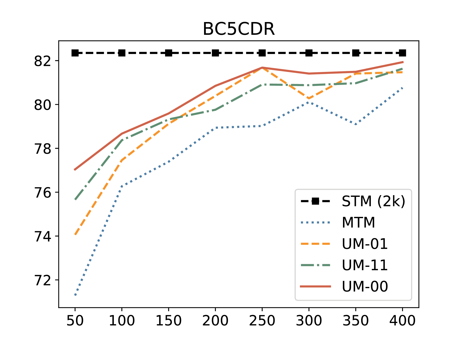
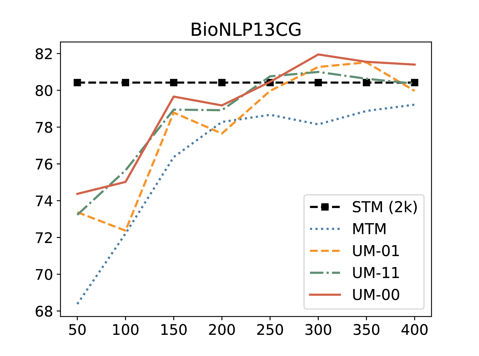
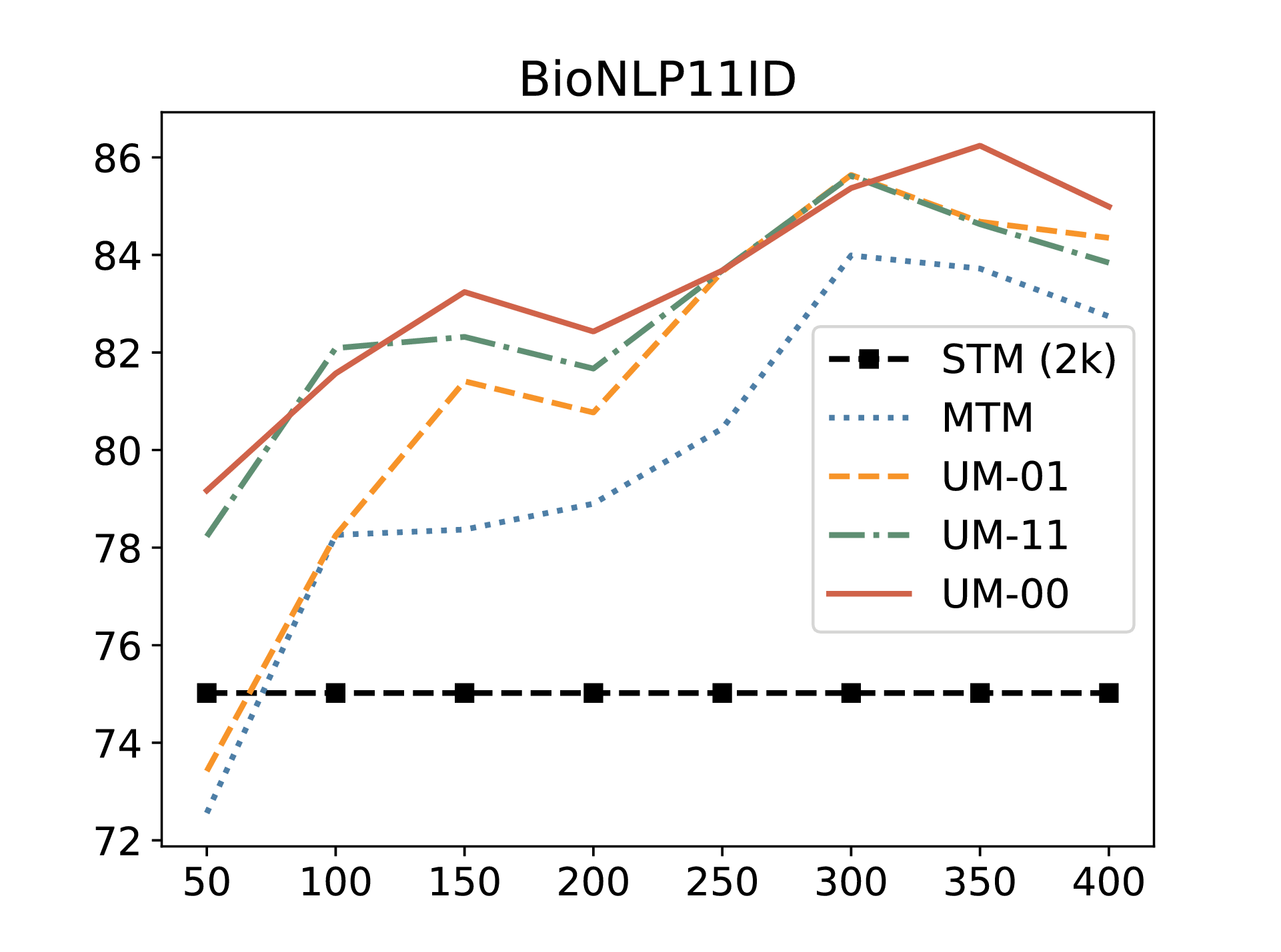
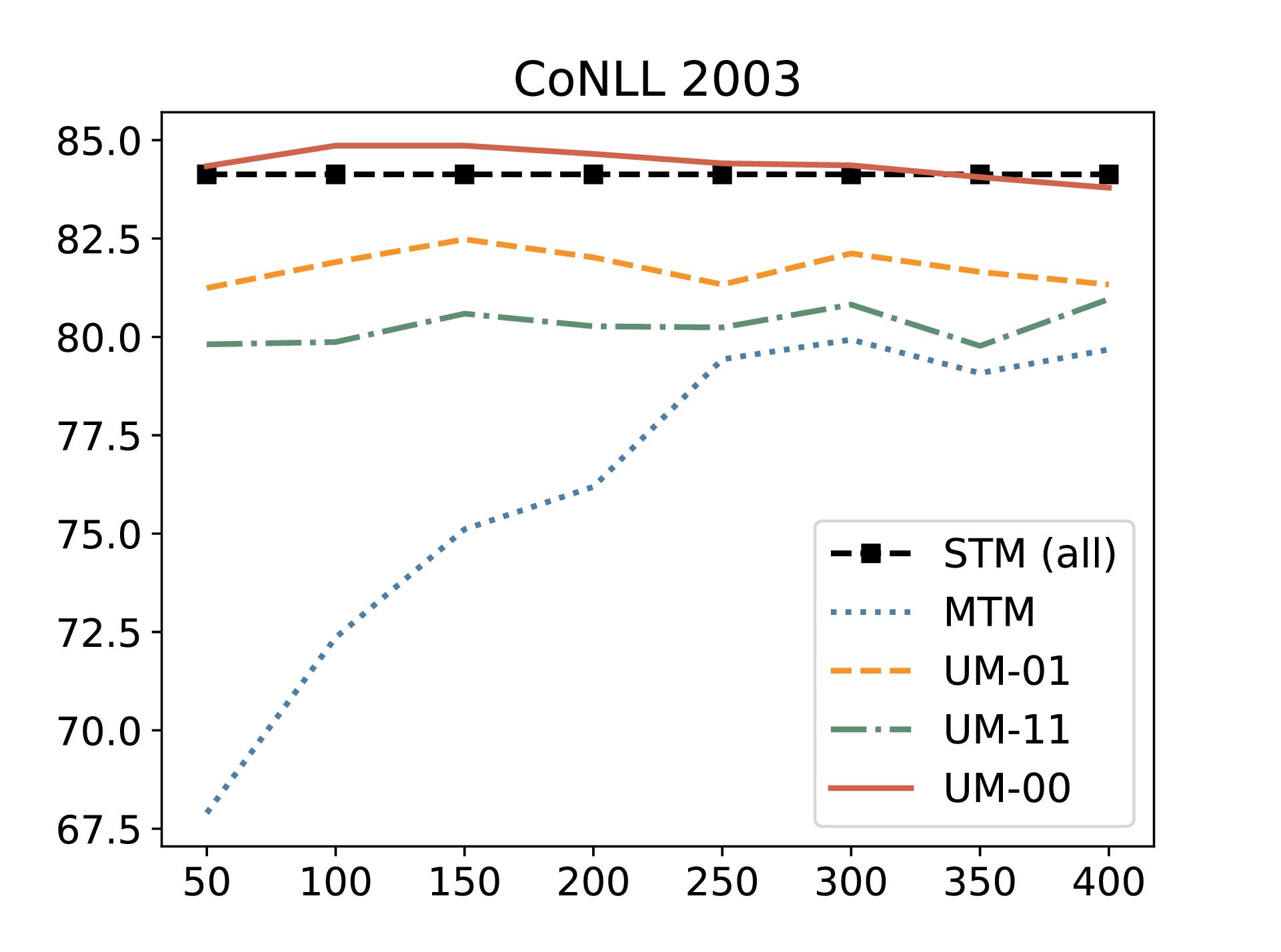
Figure 4: Plot of f1 scores for task adaptation in the limited-supervision setting. X-axis represents the number of sentences used for fine-tuning. STM(2k) is a STM trained on 2k sentences sampled from the global corpus, and STM(all) is trained on the entire training set of the corpus.

6 Results

As mentioned above, we compare the results of four different approaches in no-supervision and limited-supervision settings, both with real-world biomedical data and synthetic news data.

As a sanity check, we also evaluate the models on the test sets of the training corpora. The results can be found in Appendix A.2. It is shown that our MTM performs comparably with state-of-the-art systems evaluated on the training corpora, and thus is a strong baseline.

6.1 No-Supervision Setting

Table 2 demonstrates the results for task adaptation in the no-supervision setting. We report precision and recall in addition to f1 scores to better show the differences between the models.

Comparing on f1 scores, Unified-00 (our new model) significantly outperforms all other models on three out of four datasets, demonstrating its effectiveness. Unified-11 also achieves good results, with higher recall but lower precision than Unified-00. This aligns well with our hypothesis that it encourages predictions of entities. Conversely, Unified-01 (the naive approach) achieves the highest precision but lowest recall, which is reasonable considering the problem of false penalties that discourages the model from predicting entities. We also found that the model achieves better performance when $M=M^{\prime}$, which supports our hypothesis in 4.5 that the model works better with a valid likelihood function.

6.2 Limited-Supervision Setting

To further demonstrate the models’ ability to adapt to new datasets with a small amount of supervision, we sample a small subset of the training portion of each global evaluation corpus to fine-tune the trained models. We show the performance of the models fine-tuned with different amounts of sampled data. For each global corpus, we show a single-task model (STM) trained on it with a reasonable amount of data (two thousand sentences for the biomedical corpora). In the CoNLL 2003 setting, we train the STM on the entire training data for a fair comparison, because all other models are first trained on the four training portions, which essentially look through the entire training set (just partially annotated). The results of the STMs are used as benchmarks. Experimental results are presented in Figure 4.

Firstly, with much less training data, all the models achieve comparable or noticeably better performance than the STMs trained from scratch, demonstrating that training on the partially annotated corpora does help to boost performance on global evaluation corpora. Additionally, MTMs are worse than all the unified models, because they only share the LSTM layers, but lose all the knowledge in the CRFs when adapted to new corpora. The unified models have the advantage that they can reuse the robust CRFs learned from a large amount of data. This is more obvious in the CoNLL 2003 evaluation setting, where the unified models that reuse the pre-trained CRFs achieve good performance trained with only 50 sentences, but the MTM, which does not reuse the CRFs, needs a larger amount of training data to catch up.

In general, Unified-00, our novel approach proposed here, still performs the best on every dataset. We note that although Unified-01 has an extremely low recall on the CoNLL 2003 dataset in the no-supervision setting, it works surprisingly well in the limited-supervision setting. On the other hand, Unified-00 and Unified-11 generally perform better than Unified-01 on real-world biomedical datasets, especially when fine-tuned on less data. Again, since all the unified models are special cases of our proposed framework, we argue that, for adapting to new datasets, people can simply tune the discounting factors $M$ and $M^{\prime}$ to get good results.

7 Conclusion and Future Work

In this paper, we propose a unified model that learns from multiple partially annotated datasets to make joint predictions on the union of entity types appearing in any training dataset. The model integrates learning signals from different datasets and avoids potential conflicts that would result from combining independent predictions from multiple models. Experiments show that the proposed unified model can efficiently adapt to new corpora that have more entity types than any of the training corpora, and performs better than the baseline approaches.

In future work, we plan to explore other algorithms (e.g. imitation learning) that allow the model the explore the unknown space during training, using delayed rewards to decide whether the model should trust its exploration. Analysis of the global evaluation results suggests that the unified model is under-predicting, meaning there is still room for improvement specifically on recall. We plan to explore further changes to the current objectives to encourage more entity predictions.

Finally, the approach proposed in this paper also does not handle entity types of varying granularities or tagsets with mismatched guidelines (e.g. one dataset annotates only for-profit companies as ORG and one annotates all formalized groups). Effectively modeling these complications is an interesting area for future work.

Appendix A Appendix

A.1 Datasets

Corpus	Named Entities	Sents	Tokens	Mentions
BC2GM	Gene/Protein	20,131	569,912	24,585
BC4CHEM	Chemical	87,685	2,544,305	84,312
NCBI	Disease	7,287	184,167	6,883
JNLPBA	Gene/Protein, DNA, Cell-type, Cell-line, RNA	24,806	595,994	59,965
Linnaeus	Species	23,155	539,428	4,265

Table 3: Statistics for the Training Corpora

Corpus	Named Entities	Sents	Tokens	Mentions
BC5CDR	Chemical, Disease	13,938	360,373	28,789
BioNLP13CG	Gene/Protein, Disease, Chemical, Others	1,906	52,771	6881
BioNLP11ID	Gene/Protein, Chemical, Others	5178	166416	11084

Table 4: Statistics for global evaluation corpora. “Others” denote the NEs which do not appeared in training data, thus are not evaluated.

Below we introduce the datasets in the biomedicine domain and the news domain.

A.1.1 Biomedicine domain: Local training group

The training group consists of five datasets: BC2GM, BC4CHEM, NCBI-disease, JNLPBA, and Linnaeus. The first two datasets are from different BioCreative shared tasks Smith et al. (2008); Krallinger et al. (2015); Wei et al. (2015). NCBI-disease is created by Doğan et al. (2014) for disease name recognition and normalization. JNLPBA comes from the 2004 shared task from joint workshop on natural language processing in biomedicine and its applications Kim et al. (2004), and Linnaeus is a species corpus composed by Gerner et al. (2010). More information about the datasets can be found in Table 3.

Below are detailed descriptions of the datasets:

BC2GM is a gene/protein corpus. The annotation is Gene. It’s provided by the BioCreative II Shared Task for gene mention recognition.

BC4CHEM is a chemical corpus. The annotation is Chemical. It’s provided by the BioCreative IV Shared Task for chemical mention recognition.

NCBI-disease is a disease corpus. The annotation is Disease. It was introduced for disease name recognition and normalization.

JNLPBA consists of DNA, RNA, Gene/Protein, Cell line, Cell Type. The annotation is same as the NE names, except the Gene/Protein is annotated with Protein. It was provided by 2004 JNLPBA Shared Task for biomedical entity recognition.

Linnaeus is a species corpus. The annotation is Species. The original project was created for entity mention recognition.

	Articles	Sentences	Tokens
Training set	946	14,987	203.621
Development set	216	3,466	51,362
Test set	231	3,684	46,435

Table 5: Statistics for the CoNLL 2003 NER dataset

Corpus	BC2GM	BC4CHM	NCBI	JNLPBA	Linnaeus
STM	79.9	88.6	84.1	72.7	87.3
MTM Crichton et al. (2017)	73.2	83.0	80.4	70.1	84.0
MTM Wang et al. (2018)	80.7	89.4	86.1	73.5	-
MTM (ours)	80.3	89.2	85.8	73.5	88.5
Unified-01	70.9	83.5	79.8	80.9	79.9
Unified-11	74.2	84.1	80.5	80.9	80.7
Unified-00	79.1	87.3	84.0	83.8	83.9

Table 6: Local evaluation (f1 scores). The best results that are significantly better than the second best are bold-faced, while those are best but not significantly better than the second best are underlined. All the significance tests are conducted using mention-level McNemar’s Chi-square test, with p-value $=$ 0.01.

A.1.2 Biomedicine domain: Global evaluation group

We reemphasize here that the purpose of the global evaluation is to test the model’s ability to making global predictions and efficiently adapt to global corpora. While no corpus is globally annotated, we identify several existing corpora to approximate the global evaluation. Each test corpus is annotated with a superset of several training corpora to test the model’s generalizability outside of the local tag spaces.

The global evaluation group contains three datasets: BC5CDR, BioNLP13CG, and BioNLP11ID. Each is annotated with multiple entity types. BC5CDR comes from the BioCreative shared tasks Smith et al. (2008); Krallinger et al. (2015); Wei et al. (2015). BioNLP13CG and BioNLP11ID come from the BioNLP shared task Kim et al. (2013). More information about the global evaluation datasets can be found in Table 4.

Below are detailed descriptions of the datasets:

BC5CDR is a chemical and disease corpus. The annotation is Chemical and Disease. It’s provided by BioCreative V Shared Task for chemical and disease mention recognition.

BioNLP13CG consists of Gene/Protein and Related Product, Cancel, Chemical, Anatomy and Organism and others. BioNLP11ID consists of Gene/Protein, Chemical, and Organism. The annotation is same as the NE types but has a finer ontology scope.

There are inconsistencies between the entity type names in different datasets, mainly due to different granularities. To remove this unnecessary noise, we manually merged some entity types. For example, we unify Gene and Protein into Gene/Protein as they are commonly used interchangeably; we merge “Simple Chemical” to “Chemical” and leave the problem of entity type granularity for future work. The information in Table 3 and 4 reflects the merged types.

A.1.3 News domain: CoNLL 2003 NER dataset

We use the CoNLL 2003 NER dataset (Sang and De Meulder (2003)) to evaluate the models in news domain. More information about the dataset can be found in Table 5. We use synthetic data from the dataset to simulate local training and global evaluation. Specifically, the CoNLL 2003 NER dataset is annotated with four entity types: location, person, organization, and miscellaneous entities. We randomly split the training set into four portions, each contains only one entity type respectively, with other types changed to ”O”. The models are trained on the four training portions and we test on the original test set with all entity types annotated.

A.1.4 Data split

For the news domain, we use the default train, dev, test portion of the CoNLL 2003 NER dataset. For the biomedicine domain, we follow the data split in Crichton et al. (2017) for both the training and the evaluation groups. All datasets are divided into three portions: train, dev, and test. We train the model on the training set of the training group and tune the hyper-parameters on the corresponding development set. Global evaluations are performed on the test set of the evaluation group.

A.2 Local Evaluation

For a sanity check, we evaluate the models on the training corpora and compare the results with state-of-the-art systems. In this setting, all the models are trained on the training set of the training corpora (without fine-tuning on global evaluation corpora) and evaluated on their test set. The results are shown in Table 6. STM is the single-task models we implemented, following the settings in Wang et al. (2018). The SOTA is achieved by Wang et al. (2018) with multi-task model, which is shown in the table as MTM Wang et al. (2018). They trained their model on BC2GC, BC4CHM, NCBI, JNLPBA, and BC5CDR. MTM (ours) is the multi-task model we trained on our five training corpora and used as a baseline in the global evaluations. It has the same architecture as Wang et al. (2018).

As we can see, MTM Wang et al. (2018) achieves the best results on 3 out of 4 datasets. And our MTM achieves very similar results, showing it is a strong model on training corpora. Our proposed models do not perform very well when evaluated on the training corpora. But in the global evaluation setting, they perform much better compared to our strong MTM. This demonstrates the superiority of our proposed models on task adaptation.

References

- Aguilar et al. (2014) Jacqueline Aguilar, Charley Beller, Paul McNamee, Ben V. Durme, Stephanie Strassel, Zhiyi Song, and Joe Ellis. 2014. A comparison of the events and relations across ACE, ERE, TAC-KBP, and FrameNet annotation standards. In ACL Workshop: EVENTS.
- Bellare and McCallum (2007) Kedar Bellare and Andrew McCallum. 2007. Learning extractors from unlabeled text using relevant databases. In Sixth international workshop on information integration on the web.
- Bengio et al. (1994) Yoshua Bengio, Patrice Simard, and Paolo Frasconi. 1994. Learning long-term dependencies with gradient descent is difficult. IEEE Transactions on Neural Networks.
- Carlson et al. (2009) Andrew Carlson, Scott Gaffney, and Flavian Vasile. 2009. Learning a named entity tagger from gazetteers with the partial perceptron. In AAAI Spring Symposium: Learning by Reading and Learning to Read.
- Consortium (2013) Linguistic Data Consortium. 2013. DEFT ERE annotation guidelines: Relations v1.1. Linguistic Data Consortium, Philadelphia.
- Craven and Kumlien (1999) Mark Craven and Johan Kumlien. 1999. Constructing biological knowledge bases by extracting information from text sources. In ISMB.
- Craven et al. (1998) Mark Craven, Andrew McCallum, Dan PiPasquo, Tom Mitchell, and Dayne Freitag. 1998. Learning to extract symbolic knowledge from the world wide web. Technical report, Carnegie-mellon univ pittsburgh pa school of computer Science.
- Crichton et al. (2017) Gamal Crichton, Sampo Pyysalo, Billy Chiu, and Anna Korhonen. 2017. A neural network multi-task learning approach to biomedical named entity recognition. BMC bioinformatics.
- Doğan et al. (2014) Rezarta Islamaj Doğan, Robert Leaman, and Zhiyong Lu. 2014. Ncbi disease corpus: a resource for disease name recognition and concept normalization. Journal of biomedical informatics.
- Fernandes and Brefeld (2011) Eraldo R Fernandes and Ulf Brefeld. 2011. Learning from partially annotated sequences. In Joint European Conference on Machine Learning and Knowledge Discovery in Databases, pages 407–422. Springer.
- Gerner et al. (2010) Martin Gerner, Goran Nenadic, and Casey M Bergman. 2010. Linnaeus: a species name identification system for biomedical literature. BMC bioinformatics.
- Greenberg et al. (2018) Nathan Greenberg, Trapit Bansal, Patrick Verga, and Andrew McCallum. 2018. Marginal likelihood training of bilstm-crf for biomedical named entity recognition from disjoint label sets. In Proceedings of the 2018 Conference on Empirical Methods in Natural Language Processing, pages 2824–2829.
- Hasegawa et al. (2004) Takaaki Hasegawa, Satoshi Seki, and Ralph Grishman. 2004. Discovering relations among named entities from large corpora. In ACL.
- Hochreiter and Schmidhuber (1997) Sepp Hochreiter and Jürgen Schmidhuber. 1997. Long short-term memory. Neural computation.
- Ji et al. (2010) Heng Ji, Ralph Grishman, Hoa Trang Dang, Kira Griffitt, and Joe Ellis. 2010. Overview of the tac 2010 knowledge base population track. In TAC.
- Kim et al. (2004) Jin-Dong Kim, Tomoko Ohta, Yoshimasa Tsuruoka, Yuka Tateisi, and Nigel Collier. 2004. Introduction to the bio-entity recognition task at jnlpba. In JNLPBA. ACL.
- Kim et al. (2013) Jin-Dong Kim, Yue Wang, and Yamamoto Yasunori. 2013. The genia event extraction shared task, 2013 edition-overview. In BioNLP Shared Task 2013 Workshop.
- Krallinger et al. (2015) Martin Krallinger, Florian Leitner, Obdulia Rabal, Miguel Vazquez, Julen Oyarzabal, and Alfonso Valencia. 2015. Chemdner: The drugs and chemical names extraction challenge. Journal of Cheminfo.
- Lafferty et al. (2001) John Lafferty, Andrew McCallum, and Fernando CN Pereira. 2001. Conditional random fields: Probabilistic models for segmenting and labeling sequence data. In ICML.
- Lample et al. (2016) Guillaume Lample, Miguel Ballesteros, Sandeep Subramanian, Kazuya Kawakami, and Chris Dyer. 2016. Neural architectures for named entity recognition. In NAACL.
- Li and Liu (2005) Xiao-Li Li and Bing Liu. 2005. Learning from positive and unlabeled examples with different data distributions. In ECML.
- Liu et al. (2018) L. Liu, J. Shang, F. Xu, X. Ren, H. Gui, J. Peng, and J. Han. 2018. Empower Sequence Labeling with Task-Aware Neural Language Model. In AAAI.
- Liu et al. (2014) Yijia Liu, Yue Zhang, Wanxiang Che, Ting Liu, and Fan Wu. 2014. Domain adaptation for crf-based chinese word segmentation using free annotations. In Proceedings of the 2014 Conference on Empirical Methods in Natural Language Processing (EMNLP), pages 864–874. Association for Computational Linguistics.
- Lu et al. (2015) Yanan Lu, Donghong Ji, Xiaoyuan Yao, Xiaomei Wei, and Xiaohui Liang. 2015. Chemdner system with mixed conditional random fields and multi-scale word clustering. Journal of cheminformatics.
- Ma and Hovy (2016) Xuezhe Ma and Eduard Hovy. 2016. End-to-end sequence labeling via bi-directional lstm-cnns-crf. In ACL.
- McCallum and Li (2003) Andrew McCallum and Wei Li. 2003. Early results for named entity recognition with conditional random fields, feature induction and web-enhanced lexicons. In NAACL.
- Mooney and Bunescu (2005) Raymond J Mooney and Razvan C Bunescu. 2005. Subsequence kernels for relation extraction. In NIPS.
- Neves et al. (2012) Mariana Neves, Alexander Damas, Andreas Kurtz, and Ulf Leser. 2012. Annotating and evaluating text for stem cell research. In BioTxtM workshop at LREC on Building and Evaluation Resources.
- Peng and Dredze (2015) Nanyun Peng and Mark Dredze. 2015. Named entity recognition for chinese social media with jointly trained embeddings. In Proceedings of the 2015 Conference on Empirical Methods in Natural Language Processing (EMNLP), Lisboa, Portugal.
- Peng and Dredze (2016) Nanyun Peng and Mark Dredze. 2016. Improving named entity recognition for chinese social media via learning segmentation representations. In ACL.
- Peng and Dredze (2017) Nanyun Peng and Mark Dredze. 2017. Multi-task domain adaptation for sequence tagging. In Proceddings of the ACL Workshop on Representation Learning for NLP.
- Pyysalo and Ananiadou (2013) Sampo Pyysalo and Sophia Ananiadou. 2013. Anatomical entity mention recognition at literature scale. Bioinformatics.
- Ritter et al. (2011) Alan Ritter, Sam Clark, Oren Etzioni, et al. 2011. Named entity recognition in tweets: an experimental study. In EMNLP.
- Sang and De Meulder (2003) Erik F Sang and Fien De Meulder. 2003. Introduction to the conll-2003 shared task: Language-independent named entity recognition. arXiv preprint cs/0306050.
- Shang et al. (2018) Jingbo Shang, Liyuan Liu, Xiang Ren, Xiaotao Gu, Teng Ren, and Jiawei Han. 2018. Learning named entity tagger using domain-specific dictionary. arXiv preprint arXiv:1809.03599.
- Smith et al. (2008) Larry Smith, Lorraine K Tanabe, Rie Johnson nee Ando, Cheng-Ju Kuo, I-Fang Chung, Chun-Nan Hsu, Yu-Shi Lin, Roman Klinger, Christoph M Friedrich, Kuzman Ganchev, et al. 2008. Overview of biocreative ii gene mention recognition. Genome biology.
- Soon et al. (2001) Wee Meng Soon, Hwee Tou Ng, and Daniel Chung Yong Lim. 2001. A machine learning approach to coreference resolution of noun phrases. Computational linguistics.
- Tjong Kim Sang and De Meulder (2003) Erik F Tjong Kim Sang and Fien De Meulder. 2003. Introduction to the conll-2003 shared task: Language-independent named entity recognition. In CoNLL at HLT-NAACL.
- Tsuboi et al. (2008) Yuta Tsuboi, Hisashi Kashima, Shinsuke Mori, Hiroki Oda, and Yuji Matsumoto. 2008. Training conditional random fields using incomplete annotations. In Proceedings of the 22nd International Conference on Computational Linguistics (Coling 2008), pages 897–904. Coling 2008 Organizing Committee.
- Walker et al. (2006) Christopher Walker, Stephanie Strassel, Julie Medero, and Kazuaki Maeda. 2006. Ace 2005 multilingual training corpus. LDC.
- Wang et al. (2018) Xuan Wang, Yu Zhang, Xiang Ren, Yuhao Zhang, Marinka Zitnik, Jingbo Shang, Curtis Langlotz, and Jiawei Han. 2018. Cross-type biomedical named entity recognition with deep multi-task learning. CoRR.
- Wei et al. (2015) Chih-Hsuan Wei, Yifan Peng, Robert Leaman, Allan Peter Davis, Carolyn J Mattingly, Jiao Li, Thomas C Wiegers, and Zhiyong Lu. 2015. Overview of the biocreative v chemical disease relation (cdr) task. In BC V Workshop.
- Yang and Vozila (2014) Fan Yang and Paul Vozila. 2014. Semi-supervised chinese word segmentation using partial-label learning with conditional random fields. In EMNLP.
- Yang et al. (2018) Yaosheng Yang, Wenliang Chen, Zhenghua Li, Zhengqiu He, and Min Zhang. 2018. Distantly supervised ner with partial annotation learning and reinforcement learning. In Proceedings of the 27th International Conference on Computational Linguistics, pages 2159–2169.