Efficient Pilot Allocation for URLLC Traffic
in 5G Industrial IoT Networks

Abstract

In this paper we address the problem of resource allocation for alarm traffic in industrial Internet of Things networks using massive MIMO. We formulate the general problem of how to allocate pilot signals to alarm traffic such that delivery is guaranteed, while also minimising the number of pilots reserved for alarms, thus maximising the channel resources available for other traffic, such as industrial control traffic. We present an algorithm that fulfils these requirements, and evaluate its performance both analytically and through a simulation study. For realistic alarm traffic characteristics, on average our algorithm can deliver alarms within two time slots (of duration equal to the 5G transmission time interval) using fewer than 1.5 pilots per slot, and even in the worst case it uses around 3.5 pilots in any given slot, with delivery guaranteed in an average of approximately four slots.

I Introduction

Ultra-reliable and Low Latency Communication (URLLC) is one of the target use cases for 5G [1]. However, the performance requirements for this type of traffic are not yet met for challenging use cases such as the industrial Internet of Things (IoT). Moreover, little work has been done on the medium access control (MAC) layer of massive multiple-input multiple-out (MIMO) [2], a key technology for 5G, and mechanisms for URLLC traffic are lacking.

In this paper, we present a MAC scheme for alarm traffic in industrial control networks based on massive MIMO. In massive MIMO, pilots — known signals needed to obtain channel state information (CSI) for each user [2] — are a limited resource. We formulate the general problem of allocation of pilot signals to alarm sources, which trigger alarms when unusual events occur, for example machine failures or control values detected outside of a specified safe parameter range. We present an algorithm for efficient pilot allocation that guarantees alarm delivery. We performed a simulation study which shows good performance of our algorithm, with varying numbers of alarms and alarm trigger probabilities. In the average case, for an alarm trigger probability of $1$% per alarm and slot, less than 1.5 pilots per time slot needed to be reserved for alarm traffic, and alarms were delivered within two slots. In the worst case, alarms are delivered within an average of just over $4$ slots, with at most $3.5$ pilots needed per slot. The length of a time slot in our scheme is equal to the transmission time interval, which in 5G can be as short as 125 $\mu$s [3].

With the rise of Industry 4.0 comes a greater need for flexibility in manufacturing and other industrial processes [4, 5]. Key features of Industry 4.0 include optimisation and customisation of production, automation and adaption, and automatic data exchange and communication, while real-time capability, decentralisation, and modularity are some of the important operating principles [5]. These trends will be facilitated by the transition to wireless communications for industrial control processes, allowing for cheaper and more scalable communications, with reduced cabling costs and the ability to easily reconfigure the factory floor. However, as yet, the development and deployment of wireless protocols suitable for real-time communication in this context is limited, since existing protocols are not able to meet the stringent requirements of industrial control traffic in terms of latency and allowable packet loss rates [6, 7].

Massive MIMO is a promising technology in this domain. Diversity gain can greatly increase the reliability of communications for industrial systems [8]; for example, with no diversity gain, a $90$ dB margin is needed in the fading gain in order to reach a channel outage probability suitable for factory or process automation, while with a diversity order of 15, this is reduced to $9$ dB. In massive MIMO, the use of up to hundreds of antennas inherently provides a high degree of spatial diversity, equal to the number of antennas when using maximum ratio combining, or the number of antennas minus the number of concurrent users for zero forcing [2]. Moreover, an effect known as channel hardening [9, 10] makes massive MIMO channels behave more like wired channels, smoothing out channel variations and providing predictable performance. This effect is facilitated by low correlation between the channels of different users. The otherwise challenging radio environment of a factory [8] is thus turned into a strength, as its metallic fixtures and moving machine tools and robots provide a rich multipath channel propagation environment that aids the differentiation of user signals in massive MIMO systems.

In order to take advantage of the benefits promised by massive MIMO for industrial communications, suitable MAC protocols are needed. However, thus far, work on massive MIMO MAC for the IoT is limited, especially when it comes to URLLC. A few recent works consider random access and/or grant-free protocols for massive MIMO in IoT scenarios [11, 12, 13]. In particular, [14] argues for the advantages of massive MIMO over other technologies in the presence of massively many devices, each only transmitting intermittently. Scheduled access for periodic IoT traffic has also been considered in [15]. However, none of these works cater to the particular needs of industrial control traffic, in terms of packet loss and latency guarantees, which we address in this paper.

The rest of this paper is organised as follows. In Section II, we formulate the pilot allocation problem and define our traffic model and performance requirements. Section III then presents our pilot allocation algorithm based on a new concept that we call collision trees. Section IV details our simulation-based performance study and results, and finally Section V concludes this paper.

II Pilot Allocation for Alarm Traffic

The problem we will address is pilot allocation for alarm traffic in a 5G industrial Internet of Things scenario. Typically, in such a use case a dedicated network (or network slice) would be used, and so we do not consider traffic for other applications. In this scenario, a massive MIMO base station provides communications for both continuous control traffic and sporadic, but critical, alarm traffic. In order to communicate, both these traffic classes must be allocated pilot signals, in such a way as to guarantee the delivery of alarms, while also maintaining high performance for the control traffic.

II-A Massive MIMO Transmission

Here we will provide a brief overview of transmission in massive MIMO systems; a more comprehensive treatment can be found in [2]. Transmission in time division duplex-based massive MIMO occurs in coherence blocks, consisting of a time interval and frequency band across which the channel is constant, to within a small margin of error. Each coherence block contains a number of channel resource elements, which can each be used for downlink or uplink data, or (uplink) pilot signals. Pilot signals are used to measure channel state information for each user, and must be orthogonal. The CSI is then fed into the preprocessing matrix used to direct each data stream to its respective recipient on the downlink. or differentiate each incoming data stream on the uplink.

If two users transmit the same pilot signal in the same coherence block, the CSI for these users will be inaccurate and data to or from them will be encoded or decoded incorrectly. This phenomenon is known as pilot contamination, and effectively results in a collision between the user transmissions in the same way as interference in single-antenna wireless systems does. Collisions can be avoided by allocating each user a unique, orthogonal pilot, but for sporadic alarm traffic, this would result in a very inefficient use of resources, since most of the time these pilots will go unused.

One key difference between collisions due to pilot contamination and collisions in single-antenna systems is that with the former, the base station is able to communicate to all users involved in a collision via a multicast transmission using their combined CSI; effectively, the contaminated pilot provides CSI for all the involved users as a group. If the users in the group have very different received power, some of them may fail to receive such a transmission, however, in our scenario this is unlikely, since we have small, indoor cells and so no user will be very far from the base station. Multicast transmissions to a specific group of users involved in a collision give us new possibilities to handle collisions, for example by allocating dedicated resources (pilots) for collision resolution. In our proposed algorithm in Section III, we will make use of this capability.

II-B Traffic Classes and Requirements

Efficient pilot allocation depends on the traffic to be served, so as to strike the right balance between wastage of resources due to collisions and that due to unused pilots. In our scenario, the traffic consists of two classes: control traffic and alarm traffic. Control traffic encompasses the transmissions between machines on the factory floor and their controllers. This traffic is regular, in some cases even deterministic, and has stringent latency requirements in order to arrive within a specified control loop period. In this work, however, alarm traffic will be the main focus, while control traffic will be regarded as base load traffic, for which we will evaluate the performance impact of serving the alarm traffic. Alarms are infrequent and unpredictable, but nonetheless must be delivered reliably, making resource allocation for alarm traffic challenging. Our goal is thus to provide delivery guarantees for alarm traffic, while minimising the pilot resources required to do so.

There are two key performance requirements for industrial automation traffic, latency and packet loss probability, and their values depend on the specific industrial automation domain. The domains we will focus on are process automation, with an update frequency of 10 to 1000 ms, and factory automation, with an update frequency of 500 $\mu$s to 100 ms [7]. These two domains are of interest in this work because their update frequencies are sufficiently fast to require pilot allocation strategies that cater specifically to them, while also slow enough to be feasible to realise using the 5G transmission time interval, which ranges from 125 $\mu$s to 1 ms [3].

The packet loss rate required for our targeted domains is $1\times 10^{-9}$ [7]. This extremely low loss rate includes all potential causes of packet loss, so we will aim for 100% delivery guarantees in our pilot allocation strategy; that is, no packet should be lost due to a failure in resource allocation (after collision resolution). The packet loss rate and latency requirements should thus be considered jointly, as they are inherently tied together by the pilot allocation scheme. Packet loss can still occur for other reasons, such as noise, but this is beyond the scope of the current work.

II-C Alarm Traffic Model

The performance of any given pilot allocation strategy depends on the characteristics of the alarm traffic. We will adopt the following alarm traffic model. We define a window consisting of $T$ time slots. Each slot represents one coherence interval, in which there may be multiple coherence blocks at different frequencies. Within each slot, there are $P$ pilots available in total, and each pilot can be assigned to one or more users for that slot. If two or more users are assigned the same pilot in a given slot, a collision can occur if both of them transmit during the slot. A pilot can also be unused (wasted) if its assigned user(s) do not transmit in the slot.

We have a set $\mathcal{A}$ of alarm sources, each of which represents one type of alarm that can arise during the window. The window should be limited in time, as defined above, for two reasons. First, the set of alarms that may occur can change over time, for example when the factory floor is reconfigured. Second, the time scale at which alarms need to be served may be very different to that at which they are reset. For example, an alarm may be triggered upon the malfunction of a given machine, necessitating that the machine be shut down quickly. However, the time to repair the machine may be much longer, and while the machine is nonoperational, it is no longer possible for that alarm to be triggered again. The window should therefore be an interval in time in which the set of possible alarms is constant.

Each alarm $a\in\mathcal{A}$ has a probability $p(a)$ to be triggered during each slot, but once triggered, an alarm cannot be triggered again within the window. While in reality, alarm trigger probabilities could be correlated, we begin by assuming independent alarms to simplify the analysis, and will consider correlated alarms in future work. Each triggered alarm also has a deadline: a number of slots within which it must be successfully received by the base station. If a given alarm is not successful on its first transmission attempt, for example if there was a collision, it will attempt retransmission up until its deadline according to the pilot allocation scheme. We assume that all alarm messages are short enough to be transmitted within a single slot.

II-D Pilot Allocation Problem

Our problem is then to define a pilot allocation scheme that guarantees delivery of all alarms within their deadlines. A naive strategy could be to simply assign one pilot to each alarm, in every slot. This would certainly guarantee alarm delivery, but would be very inefficient since the probability of any alarm being triggered at all is very low, let alone in a given slot. Moreover, if there are many possible alarms, then there may not be enough pilots in each slot to uniquely assign one to each alarm source. Our goal will therefore be to minimise the number of pilots that need to be assigned to alarms, while still guaranteeing delivery.

Formally, we can define a pilot allocation scheme as a finite sequence of pilots defined for each alarm source. A given alarm source, when its alarm is triggered, begins by transmitting the alarm message in the next slot using the first pilot in its pilot sequence. If there is a collision, it attempts retransmission in the following slot, using the second pilot in its sequence. The alarm source will know that there is a collision because it will fail to receive an acknowledgement from the base station during the downlink phase of the coherence block in which it transmits. Upon further collisions the alarm source proceeds along the sequence, one slot at a time, until it reaches the end: its final retransmission attempt. A pilot sequence may also contain blank pilots, indicating that the alarm source remains silent in the corresponding slot instead of attempting retransmission.

When a collision occurs, the base station can optionally transmit a pilot offset to all alarm sources involved in the collision, using a multicast transmission as described in Section II-A. In this case, the alarm sources add the pilot offset to the next value in their pilot sequences. For example, if alarm $a\in\mathcal{A}$ has pilot $1$ as its next allocated pilot, and alarm $b\in\mathcal{A}$ has pilot $2$ as its next pilot, then if the base station transmits a pilot offset of $10$, alarm $a$ will transmit using pilot $11$ in the next slot, and $b$ will transmit using pilot $12$. The pilot offset thus allows for dynamic pilot allocation by the base station, while still having fixed, pre-determined sequences for each alarm source. As we will see in Section III, this can simplify collision resolution, since each collision can be resolved in its own pilot range in parallel with any new alarm transmissions.

A sufficient condition to guarantee alarm delivery within the deadline is that each pilot sequence should be no longer than the number of slots from an alarm triggering until its deadline, and that the last pilot in each alarm’s sequence should be unique across the set of alarms. If an alarm source has a unique pilot allocated to it in a given slot, then it will be able to transmit its alarm message without any risk of a collision, thus guaranteeing delivery in that slot. Since there is no reason to continue retransmission once collision-free transmission is guaranteed, we specify that the unique pilot condition should be met for the last pilot in each sequence. Then, if the length of the sequence is no more than the number of slots until the deadline, the alarm will be sent without collision in the worst case during the last slot before the deadline.

III Pilot Allocation Using Collision Trees

In this section we will present an efficient pilot allocation algorithm that can guarantee alarm delivery. Our algorithm is based on a concept we call collision trees, a method for assigning pilot sequences to alarms such that alarms with lower trigger probabilities have longer sequences and share pilots with other alarms more often. Shared pilots entail a risk of collision, if at least two of the alarms sharing the pilot are triggered at the same time, and therefore it is beneficial for lower probability alarms to share pilots more than higher probability alarms. The authors’ Python implementation of the collision tree algorithm [16] is available for download and use under the GNU General Public License.

III-A Algorithm Description

We begin by allocating a single, common pilot for all alarms in all slots. The common pilot is used for the initial alarm transmissions of alarm sources without requiring a prior grant for channel access. In the best case, all alarms triggered in the window will arrive in different slots, and no further pilots will need to be allocated for them. as they will each transmit without collision on the common pilot.

In the event of a collision, however, we resolve the collision in its own, isolated pilot range, facilitated by the base station transmitting a pilot offset to all involved alarm sources. This allows us to consider only the alarms involved in the collision, and ignore any further alarms that arrive during collision resolution, as these will be sent using the common pilot, and then, if necessary, undergo collision resolution in a separate pilot range not affecting the original collision resolution process. This somewhat reduces the efficiency of collision resolution, however it greatly simplifies the design of the pilot allocation scheme and allows us to more easily guarantee alarm delivery. An example of pilot allocation with collision resolution is shown in Figure 1.

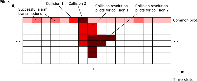
Figure 1: Example of pilot allocation for alarm transmission and collision resolution. After collision 1, four pilots are allocated in the following slot for collision resolution. This does not resolve all alarms in the collision, so a further two pilots are allocated in the next slot, after which the collision is resolved. Similarly, Collision 2 requires first four pilots, then two, then finally one in the third slot following the initial transmission.

Once a collision has occurred, the involved alarm sources attempt retransmission according to their predefined pilot sequences (see Section II-D). To design these sequences, we will use collision trees, inspired by the trees used to create Huffman codes [17]. A collision tree $\mathcal{T}=(\mathcal{V},\mathcal{E})$ is constructed as follows. We begin with the set of alarms $\mathcal{A}$, together with their trigger probabilities $p(a)$, $a\in\mathcal{A}$. Each alarm will become a leaf in the collision tree. We then combine the two alarms with the lowest probabilities, making them children of a parent node that also has a probability associated with it, namely the probability of at least one of its children (alarms) being triggered.

We then repeat the procedure, combining the two nodes with the lowest probabilities that do not yet have parent nodes, by making them children of a newly created parent node. The probability for the new node is given by the probability of at least one of the alarms in its child subtree being triggered. This process continues to iterate until finally we are left with a single node, which will become the root node of the tree, and whose probability is equal to the probability of any alarm being triggered in a given slot.

For a given node $v\in\mathcal{V}$ in the tree, the probability that at least one of the alarms in its subtree is triggered is given by

$$\pi(v)=1-\prod_{l\in\mathcal{L}(v)}\left(1-\pi(l)\right),$$ (1)

where $\mathcal{L}(v)$ is the set of leaf nodes descended from $v$, and where $\pi(l)$, for $l\in\mathcal{V}$ a leaf node of the tree, is equal to the probability of the associated alarm being triggered. That is, $\pi(l)=p(a(l))$, where $a(l)\in\mathcal{A}$ is the alarm associated with leaf node $l\in\mathcal{V}$.

Once the tree has been constructed, we need to assign pilots to each node in the tree. Each level of the tree represents one time slot in the collision resolution process, and so nodes in the tree must be assigned pilots unique within their level. This is feasible so long as the number of nodes in any level does not exceed the total number of pilots available in each time slot. To assign pilots, we simply label the nodes in each level with pilot numbers, starting from $1$ and increasing up to the number of nodes in the level. The root of the tree is assigned the common pilot for initial alarm transmissions. To determine the pilot sequence for a given alarm, we can then read, in order, the pilots assigned to each node in the path from the root to the leaf node corresponding to the alarm.

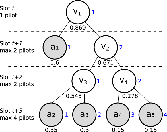
Figure 2: An example collision tree with five alarm sources. Leaf nodes representing alarms are shown in grey. Each node’s probability is shown below it, and the pilot assigned to each node is shown in blue to its right.

An example of a collision tree is shown in Figure 2, for five alarms $a_{1}\dots a_{5}$, with trigger probabilities $p(a_{1})=0.6$, $p(a_{2})=0.35$, $p(a_{3})=0.3$, $p(a_{4})=0.15$, and $p(a_{5})=0.15$. First, $a_{4}$ and $a_{5}$ are combined, since they have the lowest trigger probabilities, and placed as children of a new node $v_{4}$. The probability for $v_{4}$ is given by $\pi(v_{4})=1-(1-0.15)(1-0.15)=0.278$. The next two orphan nodes (nodes without a parent) with the lowest probabilities are then $a_{2}$ and $a_{3}$, which are placed as the children of a new node $v_{3}$, with probability $1-(1-0.3)(1-0.35)=0.545$. Now the two orphan nodes with the lowest probabilities are $v_{3}$ and $v_{4}$, so they are placed as the children of a new node $v_{2}$, with probability $1-(1-0.35)(1-0.3)(1-0.15)(1-0.15)=0.671$. Finally, we only have two orphan nodes remaining, so they are placed as the children of the new root node $v_{1}$, with probability $0.869$, which is the probability of at least one of the alarms triggering. The resulting collision tree has four levels, corresponding to a maximum of four slots needed to resolve all alarms. The maximum number of pilots that would need to be reserved in any slot is four in slot $t+3$, where $t$ is the slot in which the alarms were first transmitted.

III-B Performance Analysis

There are two key performance metrics that are of interest in assessing the quality of a given pilot allocation scheme. The first is the delivery time for the alarms, and the second is the expected number of pilots reserved for alarms, as these then cannot be used for control traffic. The delivery time can be considered both for each individual alarm, and for the entire set of alarms, by taking aggregate measures across the set. The maximum delivery time for any given alarm is given simply by the length of its pilot sequence. For collision tree-based allocation, this is equivalently the length of the path from the leaf node associated with the alarm to the root of the tree. We can express this as $\hat{D}(a)=|\mathcal{R}(l(a))|$, where $\hat{D}(a)$ is the maximum delivery time for alarm $a\in\mathcal{A}$ in time slots, $l(a)\in\mathcal{V}$ is the leaf node in the tree associated with alarm $a$, and $\mathcal{R}(v)$, $v\in\mathcal{V}$, is the path from a node $v$ to the root of the tree, consisting of the parent node of $v$, followed by the parent node of $v$’s parent, and so on up to the root node. The maximum delivery time can be used to determine whether or not alarm $a$ can be guaranteed delivery within its deadline; if $\hat{D}(a)$ is less than or equal to the number of time slots until $a$’s deadline, then delivery within the deadline is ensured.

By default, our collision tree algorithm guarantees delivery of all alarms, but not necessarily within their deadlines. However, by checking the maximum delivery time of each alarm against its deadline, the tree can easily be modified to ensure all alarms meet their deadlines, albeit with some loss of performance. This can be done by moving an alarm node $l(a)$ up the tree along $\mathcal{R}(l(a))$ until $\hat{D}(a)$ is within the deadline. First $l(a)$ is moved up one level to become a sibling of its parent, with its grandparent node as its new parent. If the deadline is still not met, this procedure is repeated so that $l(a)$ next becomes a sibling of its grandparent, then its great-grandparent, and so on as needed.

In addition to the maximum delivery time, the expected delivery time for each alarm is also important. Even though the deadline represents the absolute latest time an alarm can be delivered, not all delivery times within the deadline are necessarily equal: it may be beneficial to deliver the alarm sooner rather than later. Our collision tree algorithm seeks to minimise the probability that an alarm will use its entire pilot sequence in order to be delivered, and so the expected delivery time will be significantly shorter than the maximum. Note that while delivery time is analogous to codeword length in Huffman codes, its analysis is more complicated because alarms do not always use their full pilot sequence, that is, the expected delivery time for each alarm is in general not equal to its maximum delivery time. Since Huffman codes are optimal in terms of encoded message length [17], our collision trees will also be optimal in terms of maximum delivery times of alarms, but not necessarily in terms of expected delivery time: more analysis is needed to prove or disprove this result, and will be the subject of our future work.

The expected delivery time for an alarm $a\in\mathcal{A}$ depends on the collision probabilities at each node $r\in\mathcal{R}(l(a))$ — the probability of a collision occurring on the pilot assigned to node $r$ during its slot. This probability is given by

$$c(v)=1-\smashoperator[]{\sum_{l\in\mathcal{L}(v)}^{}}\pi(l)\,\,\smashoperator[]{\prod_{m\in\mathcal{L}(v)\setminus\{l\}}^{}}\left(1-\pi(m)\right)-\smashoperator[]{\prod_{l\in\mathcal{L}(v)}^{}}\left(1-\pi(l)\right),$$ (2)

that is, the complement of the probability that either none of the alarms sharing the pilot assigned to $v$ were triggered, or only one of them was: as soon as two or more alarms transmit, a collision will occur.

However, when determining the expected delivery time of a given alarm $a$, that specific alarm must have been triggered, and so we need to find the conditional collision probability given that $a$ was triggered. In this case, it is sufficient for any one of the other alarms also covered by $v$ to be triggered, and so the conditional probability of a collision at $v$ given $a$ was triggered is

$$c(v,a)=1-\prod_{m\in\mathcal{L}(v)\setminus\{l(a)\}}\left(1-\pi(m)\right).$$ (3)

The expected delivery time for alarm $a$ is then given by

$$E\left[D(a)\right]=1+\sum_{r\in\mathcal{R}(l(a))\setminus\{v_{0}\}}c(r,a).$$ (4)

where $D(a)$ is the random variable representing the delivery time of alarm $a$, and $v_{0}$ is the root node of the tree. The minimum delivery time is always one slot, representing the case when the alarm is delivered straight away without collision. In the event of a collision, an additional slot is then added for each node along the path $\mathcal{R}(l(a)$ at which there is a collision. Note that a collision at node $v\in\mathcal{V}$ also implies a collision at all nodes along $\mathcal{R}(v)$, and the collision probability at any leaf node is $0$. Finally, in order to obtain an aggregate performance metric across all alarms, we can take the average delivery time across the alarms as

$$D=\frac{1}{|\mathcal{A}|}\sum_{a\in\mathcal{A}}E\left[D(a)\right].$$ (5)

Our second performance consideration is the effect of our pilot allocation scheme on the control traffic, in terms of the total expected number of pilots reserved for alarm traffic per slot, including pilots allocated for collision resolution. However, calculating the expected number of reserved pilots with our alarm traffic model is not straightforward, since once an alarm is triggered, it can no longer be triggered again. It is thus removed from the set of possible alarms, and consequently, the probability of a collision will be lower in subsequent slots, meaning that the expected number of reserved pilots for each slot will reduce monotonically as we move through the time window and alarms are triggered. To calculate the expectation over all slots, we would therefore need to consider all possible combinations of which alarms could trigger in the same slots, and in which order, which is not feasible to do in practice.

We will therefore take as a performance measure the a priori expected number of pilots reserved per slot, that is, the expected number of pilots needed for alarms per slot assuming all alarms can be triggered. This will give an upper bound on the true expectation where alarms can only be triggered once. The a priori expected number of pilots reserved for alarm traffic is given by

$$\hat{E}[P]=1+\sum_{v\in\mathcal{V}\setminus\{v_{0}\}}c(R(v)),$$ (6)

where $\hat{E}$ denotes the a priori expectation as defined above, $P$ is the random variable representing the number of pilots reserved for alarm traffic per slot, and $R(v)$, $v\in\mathcal{V}$, is the parent node of $v$. One pilot is needed for each node whose parent node has a collision, with an additional pilot for the root node (the common pilot reserved in all blocks for alarms).

The two performance metrics discussed here do not take into account the effect of alarms being removed from the set of possible alarms after they have been triggered, and so will overestimate the real performance. However, they provide an indication of the worst case performance, when no alarms have yet been triggered, and so assist with dimensioning the network. Further, these metrics provide a means to compare different collision trees, produced either by the algorithm given in Section III or others. For example, these metrics could be used to optimise the collision tree, which we intend to explore in our future work.

IV Simulation Study

In order to empirically test the performance of the collision tree algorithm, we implemented a simulator in Python for alarm pilot allocation, along with numerical functions for the performance metrics detailed in Section III-B. The full code is available online [16].

IV-A Simulation

The simulation proceeds as follows. First, a set of alarms $\mathcal{A}$ is generated, each $a\in\mathcal{A}$ with a per time slot trigger probability $p(a)$ between $0$ and $p$, where $p$ is a simulation parameter. We tested the following values of $p$: $0.001$, $0.005$, $0.01$, $0.05$, $0.1$, and $0.5$. While some of these trigger probabilities are unrealistically high for practical scenarios, they are useful to find the limits of the system’s capabilities. The number of alarms in $\mathcal{A}$, that is $|\mathcal{A}|$, was also varied, from $10$ to $100$ in steps of $10$. Note that this is the total number of possible alarms that can arrive, but the actual triggering of these alarms depends on the trigger probabilities and not all will necessarily be triggered during any given simulation.

For each configuration of these two parameters, $20$ problem instances (instances of $\mathcal{A}$ along with $p(a)\in[0,p]$ for each $a\in\mathcal{A}$) were generated. For each such instance, a collision tree was built from the trigger probabilities $p(a)$ using the algorithm described in Section III-A. From the collision tree, we calculated the analytical performance metrics, specifically, the average alarm delivery time (Equation (5)) and the a priori expected number of pilots used per slot (Equation (6)). Finally, the actual simulation was then run $50$ times for each instance, with a window size of $50$ slots.

During the simulation, in each slot, a random number is drawn between $0$ and $1$ for each alarm that has not yet been triggered. If this number is lower than the alarm’s trigger probability $p(a)$, the alarm is triggered in that slot. If more than one alarm is triggered, a collision occurs and is resolved using the collision tree in subsequent slots. Once the window has ended, no more alarms are triggered, but the simulation continues until all remaining collisions are resolved.

IV-B Results

A selection of simulation results are shown in Figures 3 and 4. Full results can be obtained by downloading and running the simulation code from [16]. We show here the results for $p=0.01$, which gives relatively high but nonetheless realistic trigger probabilities. For some simulations, no alarms are triggered. In these cases, both the average and maximum delivery times were set to $1.0$, as were the average and maximum pilots per slot, since an alarm always needs at least one pilot in one slot to be delivered and this thus gives a minimum value. All results are shown with $95\%$ confidence intervals,

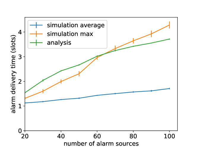
Figure 3: Delivery times for alarms with trigger probability upper bound $p=0.01$, average across all simulation runs and instances (Simulation average), maximum for each simulation run, averaged across all runs and instances (Simulation max), and analytical average delivery time $D$ (Analysis, Equation (5)).

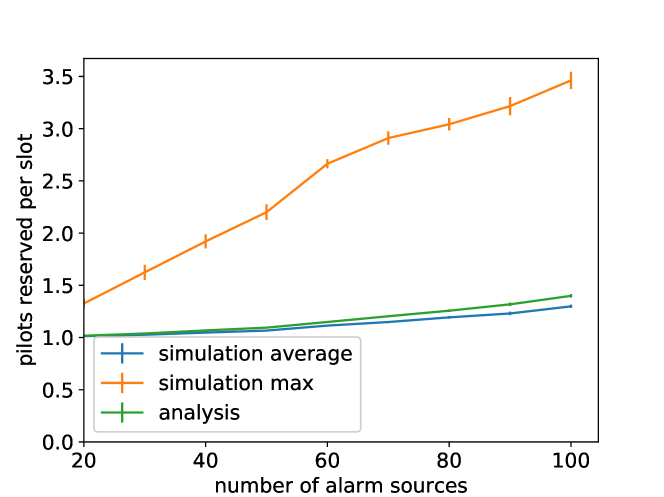
Figure 4: Pilots reserved for alarms per slot with trigger probability upper bound $p=0.01$, average across all simulation runs and instances (Simulation average), maximum for each simulation run, averaged across all runs and instances (Simulation max), and analytical average delivery time $\hat{E}[P]$ (Analysis, Equation (6)).

The maximum delivery time for a given alarm can be theoretically as high as $|\mathcal{A}|$ slots in the worst case, when the collision tree is unbalanced such that there is one leaf for each level in the tree. However, as the delivery time results (Figure 3) show, in practice the delivery times are much shorter using our collision tree algorithm, on average less than 2 slots and with a maximum of around $4$ slots for $p=0.01$. The analytical average delivery time tracked the maximum, giving an indication of the worst case performance, and it provides an upper bound for the actual average, since it does not take into account alarms being removed after they are triggered. Delivery times increased with $p$, however even for the highest value tested, $p=0.5$, and with $100$ alarms, the maximum delivery time was less than $8$ slots and the average around $4$ slots, showing that our algorithm effectively controls the delivery time even in challenging cases.

The collision tree algorithm also showed good performance with regards to the number of pilots reserved for alarms per slot (Figure 4). Here, the analytical metric $\hat{E}[P]$ followed the simulation average for low to medium values of $p$, although at higher values the analysis diverges from the simulation average. The maximum number of pilots reserved for alarms was approximately $3.5$ pilots with $100$ alarms and a maximum trigger probability of $0.01$. This shows that the disruption to control traffic is limited, even in cases where many alarms are triggered at once. Moreover, the average number of pilots reserved per slot was very low, less than $1.5$. The collision tree algorithm is thus able to guarantee alarm delivery while making very efficient use of pilot resources for realistic alarm traffic. As $p$ increases, both the average and maximum number of pilots used also increase, with a maximum number of pilots of $17.5$ for $p=0.1$ and $56$ for $p=0.5$. This gives an indication of the maximum traffic that can be accommodated by a single base station using our approach.

V Conclusion

In this paper we have studied a new problem in URLLC traffic in 5G networks, that of massive MIMO pilot allocation for alarm traffic in industrial Internet of Things scenarios, in particular factory and process automation. We have presented a grant-free random access scheme for alarm traffic, together with an algorithm for pilot collision resolution that can guarantee alarm delivery while making efficient use of pilot resources. In our future work we plan to further investigate the performance when alarm deadlines are shorter than their initial assigned pilot sequence length, necessitating moving some alarms further up the collision tree. We also aim to find optimal collision trees and compare them with those generated using our algorithm, as well as compare the performance of collision trees with other contention resolution methods. Other possible directions for future work include modelling and simulation of control traffic, as well as studying different traffic distributions for alarms and correlation between alarm sources.

References

- [1] M. Shafi, A. F. Molisch, P. J. Smith, T. Haustein, P. Zhu, P. De Silva, F. Tufvesson, A. Benjebbour, and G. Wunder, “5G: A tutorial overview of standards, trials, challenges, deployment, and practice,” IEEE Journal on Selected Areas in Communications, vol. 35, no. 6, pp. 1201–1221, 2017.
- [2] T. L. Marzetta, E. G. Larsson, H. Yang, and H. Q. Ngo, Fundamentals of Massive MIMO. Cambridge University Press, 2016.
- [3] J. Sachs, G. Wikstrom, T. Dudda, R. Baldemair, and K. Kittichokechai, “5G radio network design for ultra-reliable low-latency communication,” IEEE Network, vol. 32, no. 2, pp. 24–31, 2018.
- [4] S. Vaidya, P. Ambad, and S. Bhosle, “Industry 4.0 — a glimpse,” Procedia Manufacturing, vol. 20, no. 1, pp. 233–238, 2018.
- [5] Y. Lu, “Industry 4.0: A survey on technologies, applications and open research issues,” Journal of Industrial Information Integration, vol. 6, pp. 1–10, 2017.
- [6] M. Wollschlaeger, T. Sauter, and J. Jasperneite, “The future of industrial communication: Automation networks in the era of the internet of things and industry 4.0,” IEEE Industrial Electronics Magazine, vol. 11, no. 1, pp. 17–27, 2017.
- [7] M. Gidlund, T. Lennvall, and J. Åkerberg, “Will 5G become yet another wireless technology for industrial automation?” in 2017 IEEE International Conference on Industrial Technology (ICIT). IEEE, 2017, pp. 1319–1324.
- [8] B. Holfeld, D. Wieruch, T. Wirth, L. Thiele, S. A. Ashraf, J. Huschke, I. Aktas, and J. Ansari, “Wireless communication for factory automation: An opportunity for LTE and 5G systems,” IEEE Communications Magazine, vol. 54, no. 6, pp. 36–43, 2016.
- [9] E. G. Larsson, O. Edfors, F. Tufvesson, and T. L. Marzetta, “Massive MIMO for next generation wireless systems,” IEEE communications magazine, vol. 52, no. 2, pp. 186–195, 2014.
- [10] S. Gunnarsson, J. Flordelis, L. V. der Perre, and F. Tufvesson, “Channel hardening in massive MIMO — a measurement based analysis,” in Proc. IEEE International Workshop on Signal Processing Advances in Wireless Communications (SPAWC), June 2018, pp. 1–5.
- [11] E. Björnson, E. De Carvalho, E. G. Larsson, and P. Popovski, “Random access protocol for massive MIMO: Strongest-user collision resolution (SUCR),” in 2016 IEEE International Conference on Communications (ICC). IEEE, 2016, pp. 1–6.
- [12] J. H. Sørensen, E. De Carvalho, and P. Popovski, “Massive MIMO for crowd scenarios: A solution based on random access,” in Globecom Workshops (GC Wkshps), 2014. IEEE, 2014, pp. 352–357.
- [13] E. De Carvalho, E. Björnson, E. G. Larsson, and P. Popovski, “Random access for massive MIMO systems with intra-cell pilot contamination,” in 2016 IEEE International Conference on Acoustics, Speech and Signal Processing (ICASSP). IEEE, 2016, pp. 3361–3365.
- [14] L. Liu, E. G. Larsson, W. Yu, P. Popovski, C. Stefanovic, and E. De Carvalho, “Sparse signal processing for grant-free massive connectivity: A future paradigm for random access protocols in the internet of things,” IEEE Signal Processing Magazine, vol. 35, no. 5, pp. 88–99, 2018.
- [15] E. Fitzgerald, M. Pióro, and F. Tufvesson, “Massive MIMO optimization with compatible sets,” IEEE Transactions on Wireless Communications, vol. 18, no. 5, pp. 2794–2812, 2019.
- [16] E. Fitzgerald, “Collision tree simulator,” https://bitbucket.org/emmafitzgerald/collision-tree-simulator.
- [17] D. A. Huffman, “A method for the construction of minimum-redundancy codes,” Proceedings of the IRE, vol. 40, no. 9, pp. 1098–1101, 1952.