A Generative Model for Molecular Distance Geometry

Abstract

Great computational effort is invested in generating equilibrium states for molecular systems using, for example, Markov chain Monte Carlo. We present a probabilistic model that generates statistically independent samples for molecules from their graph representations. Our model learns a low-dimensional manifold that preserves the geometry of local atomic neighborhoods through a principled learning representation that is based on Euclidean distance geometry. In a new benchmark for molecular conformation generation, we show experimentally that our generative model achieves state-of-the-art accuracy. Finally, we show how to use our model as a proposal distribution in an importance sampling scheme to compute molecular properties.

1 Introduction

Over the last few years, many highly-effective deep learning methods generating small molecules with desired properties (e.g., novel drugs) have emerged (Gómez-Bombarelli et al., 2018; Segler et al., 2018; Dai et al., 2018; Jin et al., 2018; Bradshaw et al., 2019a; Liu et al., 2018; You et al., 2018; Bradshaw et al., 2019b). These methods operate using graph representations of molecules in which nodes and edges represent atoms and bonds, respectively. A representation that is closer to the physical system is one in which a molecule is described by its geometry or conformation. A conformation $\mathbf{x}$ of a molecule is defined by a set of atoms $\{(\epsilon_{i},\mathbf{r}_{i})\}_{i=1}^{N_{v}}$, where $N_{v}$ is the number of atoms in the molecule, $\epsilon_{i}\in\{\text{H},\text{C},\text{O},...\}$ is the chemical element of the atom $i$, and $\mathbf{r}_{i}\in\mathbb{R}^{3}$ is its position in Cartesian coordinates. Importantly, the relative positions of the atoms are restricted by the bonds in the molecule and the angles between them. Due to thermal fluctuations resulting in stretching of and rotations around bonds, there exist infinitely many conformations of a molecule. A molecule’s graph representation and a set of its conformations are shown in Fig. 1. Under a wide range of conditions, the probability $p(\mathbf{x})$ of a conformation $\mathbf{x}$, is governed by the Boltzmann distribution and is proportional to $\exp\{-E(\mathbf{x})/k_{B}T\}$, where $E(\mathbf{x})$ is the conformation’s energy, $k_{B}$ is the Boltzmann constant, and $T$ is the temperature.

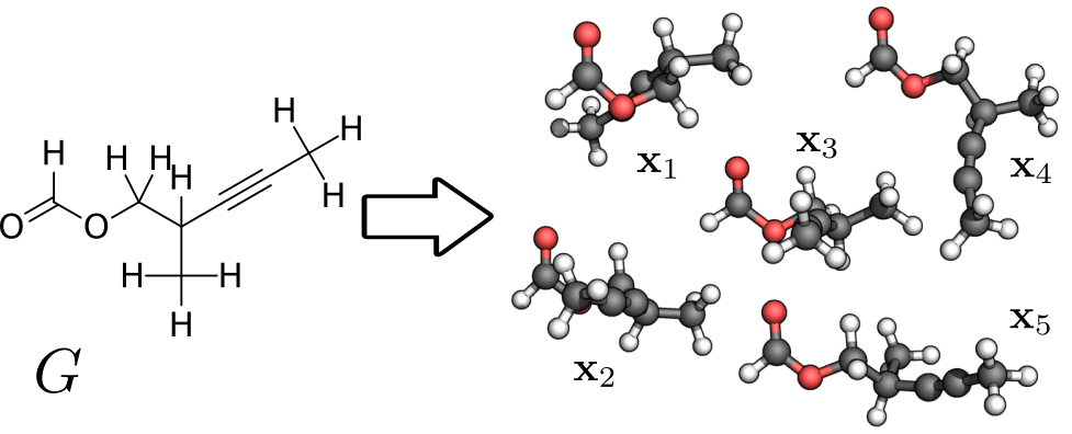
Figure 1: Standard graph representation $G$ of a molecule (left) with a set of possible conformations $\{\mathbf{x}_{i}\}$ (right). It is the goal of this work to generate such conformations from the graph representation of a molecule. Conformations feature the same atom types and bonds but the atoms are arranged differently in space. These differences arise from rotations around and stretching of bonds in the molecule. Hydrogen (H), carbon (C), and oxygen (O) atoms are colored white, gray, and red, respectively.

To compute a molecular property for a molecule, one must sample from $p(\mathbf{x})$. The main approach is to start with one conformation and make small changes to it over time, e.g., by using Markov chain Monte Carlo (MCMC) or molecular dynamics (MD). These methods can be used to accurately sample equilibrium states of molecules, but they become computationally expensive for larger ones (Shim & MacKerell, 2011; Ballard et al., 2015; De Vivo et al., 2016). Other heuristic approaches exist in which distances between atoms are set to fixed idealized values (Havel, 2002; Blaney & Dixon, 2007). Several methods based on statistical learning have also recently been developed to tackle the issue of conformation generation. However, they are mainly geared towards studying proteins and their folding dynamics (AlQuraishi, 2019). Some of these models are not targeting a distribution over conformations but the most stable folded configuration, e.g. AlphaFold (Senior et al., 2020), while others are not transferable between different molecules (Lemke & Peter, 2019; Noé et al., 2019).

This work includes the following key contributions:

• We introduce a novel probabilistic model for learning conformational distributions of molecules with graph neural networks.

• We create a new, challenging benchmark for conformation generation, which is made publicly available. To the best of our knowledge, this is the first benchmark of this kind.

• By combining a conditional variational autoencoder (CVAE) with an Euclidean distance geometry (EDG) algorithm we present a state-of-the-art approach for generating one-shot samples of molecular conformations for unseen molecules that is independent of their size and shape.

• We develop a rigorous experimental approach for evaluating and comparing the accuracy of conformation generation methods based on the mean maximum deviation distance metric.

• We show how this generative model can be used as a proposal distribution in an importance sampling (IS) scheme to estimate molecular properties.

2 Method

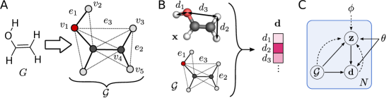
Figure 2: A) The structural formula of a molecule $G$ is converted to an extended molecular graph $\mathcal{G}$ consisting of nodes representing atoms (circles, e.g., $v_{1}$) and edges representing molecular bonds (solid lines, e.g., $e_{1}\in E_{\text{bond}}$) and auxiliary edges (dotted lines, e.g., $e_{2}\in E_{\text{angle}}$ and $e_{3}\in E_{\text{dihedral}}$). B) The distances $\mathbf{d}$ are extracted from a conformation $\mathbf{x}$ based on the edges $E$. C) Graphical model of the variational autoencoder: generative model $p_{\theta}(\mathbf{d}|\mathbf{z},\mathcal{G})p_{\theta}(\mathbf{z}|\mathcal{G})$ (solid lines) and variational approximation $q_{\phi}(\mathbf{z}|\mathbf{d},\mathcal{G})$ (dashed lines).

Our goal is to build a statistical model that generates molecular conformations in a one-shot fashion from a molecule’s graph representation. First, we describe how a molecule’s conformation can be represented by a set of pairwise distances between atoms and why this presentation is advantageous over one in Cartesian coordinates (Section 2.1). Second, we present a generative model in Section 2.2 that will generate sets of atomic distances for a given molecular graph. Third, we explain in Section 2.3 how a set of predicted distances can be transformed into a molecular conformation and why this transformation is necessary. Finally, we detail in Section 2.4 how our generative model can be used as a proposal distribution in an IS scheme to estimate molecular properties.

2.1 Extended Molecular Graphs and Distance Geometry

In this study, a molecule is represented by an undirected graph which is defined as a tuple $G=(V,E)$. $V=\{v_{i}\}_{i=1}^{N_{v}}$ is the set of nodes representing atoms, where each $v_{i}\in\mathbb{R}^{F_{v}}$ holds atomic attributes (e.g., the element type $\epsilon_{i}$). $E=\{(e_{k},r_{k},s_{k})\}_{k=1}^{N_{e}}$ is the set of edges, where each $e_{k}\in\mathbb{R}^{F_{e}}$ holds an edge’s attributes (e.g., the bond type), and $r_{k}$ and $s_{k}$ are the nodes an edge is connecting. Here, $E$ represents the molecular bonds in the molecule.

We assume that, given a molecular graph $G$, one can represent one of its conformations $\mathbf{x}$ by a set of atomic distances $\mathbf{d}=\{d_{k}\}_{k=1}^{N_{e}}$, where $d_{k}=|\mathbf{r}_{r_{k}}-\mathbf{r}_{s_{k}}|$ is the Euclidean distance between the positions of the atoms $r_{k}$ and $s_{k}$ in this conformation. As the set of edges between the bonded atoms ($E_{\text{bond}}$) alone would not suffice to describe a conformation, we expand the traditional graph representation of a molecule by adding auxiliary edges to obtain an extended graph $\mathcal{G}$. Auxiliary edges between atoms that are second neighbors in the original graph $G$ fix angles between atoms, and those between third neighbors fix dihedral angles (denoted $E_{\text{angle}}$ and $E_{\text{dihedral}}$, respectively). In this work, $E_{\text{angle}}$ are added between nodes in $\mathcal{G}$ which are second neighbors in $G$. After all $E_{\text{angle}}$ have been added, additional edges are added to $\mathcal{G}$ from a node $v$ to a randomly chosen third neighbor of $v$ in $G$ if $v$ has less then three neighbors in $\mathcal{G}$. Therefore, a graph $G$ can give rise to multiple different extend graphs $\mathcal{G}$. In Fig. 2, the process of extending the molecular graph and the extraction of $\mathbf{d}$ from $\mathbf{x}$ and $\mathcal{G}$ are illustrated.

A key advantage of a representation in terms of distances is its invariance to rotation and translation; by contrast, Cartesian coordinates depend on the (arbitrary) choice of origin, for example. In addition, it reflects pair-wise physical interactions and their generally local nature. Auxiliary edges can be placed between higher-order neighbors depending on how far the physical interactions dominating the potential energy of the system reach.

We have a set of $N_{G}$ pairs, $\{G_{i},x_{i}\}_{i=1}^{N_{G}}$, consisting of a molecular graph and a conformation. With the protocol described above, we convert each pair into a pair of an extended molecular graph together with a set of distances $\mathbf{d}$ to obtain $\{\mathcal{G}_{i},\mathbf{d}_{i}\}_{i=1}^{N_{G}}$. With this data, we will train a generative model which we detail in the following section.

2.2 Generative Model

We employ a CVAE (Kingma & Welling, 2014; Pagnoni et al., 2018) to model the distribution over distances $\mathbf{d}$ given a molecular graph $\mathcal{G}$. A CVAE first encodes $\mathcal{G}$ together with $\mathbf{d}$ into a latent space $\mathbf{z}\in\mathbb{R}^{kN_{v}}$, where $k\in\mathbb{N}^{+}$, with an encoder $q_{\phi}(\mathbf{z}|\mathbf{d},\mathcal{G})$. Subsequently, the decoder $p_{\theta}(\mathbf{d}|\mathbf{z},\mathcal{G})$ decodes $\mathbf{z}$ back into a set of distances. A graphical model is shown in Fig. 2, C.

A conformation has, in general, $3N_{v}-6$ spatial degrees of freedom (dofs): one dof per spacial dimension per atom minus three translational and three rotational dofs. Therefore, the latent space should be proportional to the number of atoms in the molecule. In addition, the latent space should be smaller than $3N_{v}$ as it is the role of the encoder to project the conformation into a lower-dimensional space. As a result, we set $k=1$.

Here, $q_{\phi}(\mathbf{z}|\mathbf{d},\mathcal{G})$ and $p_{\theta}(\mathbf{d}|\mathbf{z},\mathcal{G})$ are Gaussian distributions, the mean and variance of which are modeled by two artificial neural networks. At the center of this model are message-passing neural networks (MPNNs) (Gilmer et al., 2017). In short, an MPNN is a convolutional neural network that allows end-to-end learning of prediction pipelines whose inputs are graphs of arbitrary size and shape. In a convolution, neighboring nodes exchange so-called messages between neighbors to update their attributes. Edges update their attributes with the features of the nodes they are connecting. The MPNN is a well-studied technique that achieves state-of-the-art performance in representation learning for molecules (Kipf & Welling, 2017; Duvenaud et al., 2015; Kearnes et al., 2016; Schütt et al., 2017b; Gilmer et al., 2017; Kusner et al., 2017; Bradshaw et al., 2019a).

In the following, we describe the details of the mode which is illustrated in Fig. 3. In the encoder $q_{\phi}(\mathbf{z}|\mathbf{d},\mathcal{G})$, each $d_{k}$ is concatenated with the respective edge feature $e_{k}$ to give $e_{k}^{\prime}\in\mathbb{R}^{F_{e}+1}$. Then, each $v_{i}$ and each $e^{\prime}_{k}$ are passed to $F_{\text{enc},v}$ and $F_{\text{enc},e}$ (two multilayer perceptrons, MLPs), respectively, to give $\mathcal{G}_{\text{enc}}^{(0)}$, where $\mathcal{G}_{\text{enc}}^{(t)}=(\{v_{i,\text{enc}}^{(t)}\}_{i=1}^{N_{v}},\{(e_{k,\text{enc}}^{(t)},r_{k},s_{k})\}_{k=1}^{N_{e}})$, $v_{i,\text{enc}}^{(t)}\in\mathbb{R}^{L_{\text{v}}}$, and $e_{k,\text{enc}}^{(t)}\in\mathbb{R}^{L_{\text{e}}}$. Then, $T$ MPNNs of depth 1, $\{\text{MP}^{(t)}_{\text{enc}}\}_{t=1}^{T}$, are consecutively applied to obtain $\mathcal{G}_{\text{enc}}^{(T)}$. Finally, the read-out function $R_{\text{enc}}$ (an MLP) takes each $v_{\text{i, enc}}^{(T)}$ to predict the mean $\mu_{z_{i}}\in\mathbb{R}$ and the variance $\sigma^{2}_{z_{i}}\in\mathbb{R}$ of the Gaussian distribution for $z_{i}$. The so-called reparametrization trick is employed to draw a sample for $z_{i}$. In summary,

$$v_{i,\text{enc}}^{(0)}=F_{\text{enc},v}(v_{i}),\quad e_{k,\text{enc}}^{(0)}=F_{\text{enc},e}(e^{\prime}_{i}),$$ (1)

$$\mathcal{G}_{\text{enc}}^{(t+1)}=\text{MP}^{(t)}_{\text{enc}}(\mathcal{G}_{\text{enc}}^{(t)}),$$ (2)

$$\mu_{z_{i}},\sigma^{2}_{z_{i}}=R_{\text{enc}}(v_{i,\text{enc}}^{(T)}).$$ (3)

In the decoder $p_{\theta}(\mathbf{d}|\mathbf{z},\mathcal{G})$, each $z_{i}$ is concatenated with the respective node feature $v_{i}$ to give $v_{i}^{\prime}\in\mathbb{R}^{F_{v}+1}$. Each $v^{\prime}_{i}$ and each $e_{k}$ are passed to $F_{\text{dec},v}$ and $F_{\text{dec},e}$ (two MLPs), respectively, to give $\mathcal{G}_{\text{dec}}^{(0)}$, where $\mathcal{G}_{\text{dec}}^{(t)}=(\{v_{i,\text{dec}}^{(t)}\}_{i=1}^{N_{v}},\{(e_{k,\text{dec}}^{(t)},r_{k},s_{k})\}_{k=1}^{N_{e}})$, $v_{i,\text{dec}}^{(t)}\in\mathbb{R}^{L_{\text{v}}}$, and $e_{k,\text{dec}}^{(t)}\in\mathbb{R}^{L_{\text{e}}}$. Then, $T$ MPNNs of depth 1, $\{\text{MP}^{(t)}_{\text{dec}}\}_{t=1}^{T}$, are consecutively applied to obtain $\mathcal{G}_{\text{dec}}^{(T)}$. Finally, the read-out function $R_{\text{dec}}$ (an MLP) takes each $e_{\text{k, dec}}^{(T)}$ to predict the mean $\mu_{d_{k}}\in\mathbb{R}$ and the variance $\sigma^{2}_{d_{k}}\in\mathbb{R}$ of the Gaussian distribution for $d_{k}$. In summary,

$$v_{i,\text{dec}}^{(0)}=F_{\text{dec},v}(v^{\prime}_{i}),\quad e_{k,\text{dec}}^{(0)}=F_{\text{dec},e}(e_{i}),\\$$ (4)

$$\mathcal{G}_{\text{dec}}^{(t+1)}=\text{MP}^{(t)}_{\text{dec}}(\mathcal{G}_{\text{dec}}^{(t)}),$$ (5)

$$\mu_{d_{k}},\sigma^{2}_{d_{k}}=R_{\text{dec}}(e_{k,\text{dec}}^{(T)}).$$ (6)

The sets of parameters in the encoder and decoder, $\phi$ and $\theta$ (i.e., parameters in $F_{\text{enc},v}$, $F_{\text{enc},e}$, $\{\text{MP}^{(t)}_{\text{enc}}\}_{t=1}^{T}$, $R_{\text{enc}}$, $F_{\text{dec},v}$, $F_{\text{dec},e}$, $\{\text{MP}^{(t)}_{\text{dec}}\}_{t=1}^{T}$, $R_{\text{dec}}$), respectively, are optimized by maximizing the evidence lower bound (ELBO):

$$\begin{split}L=\mathbb{E}_{\mathbf{z}\sim q_{\phi}(\mathbf{z}|\mathbf{d},\mathcal{G})}[\log p_{\theta}(\mathbf{d}|\mathbf{z},\mathcal{G})]\\ -D_{\text{KL}}[q_{\phi}(\mathbf{z}|\mathbf{d},\mathcal{G})||p_{\theta}(\mathbf{z}|\mathcal{G})],\end{split}$$ (7)

where the prior $p_{\theta}(\mathbf{z}|\mathcal{G})$ consists of factorized standard Gaussians. The optimal values for the hyperparameters for the network dimensions, number of message passes, batch size, and learning rate of the Adam optimizer (Kingma & Ba, 2014) were manually tuned by maximizing the validation performance (ELBO) and are reported in the Appendix.

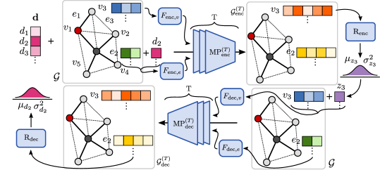
Figure 3: The molecular graph $\mathcal{G}$ together with the distances $\mathbf{d}$ are passed through the model consisting of an encoder $q_{\phi}(\mathbf{z}|\mathbf{d},\mathcal{G})$ and a decoder $p_{\theta}(\mathbf{d}|\mathbf{z},\mathcal{G})$. See Section 2.2 for details.

2.3 Conformation Generation through Euclidean Distance Geometry

To compute molecular properties, quantum-chemical methods need to be employed which require the input, i.e., the molecule, to be in Cartesian coordinates. Therefore, we use an EDG algorithm to translate the set of distances $\{d_{k}\}_{k=1}^{N_{e}}$ to a set of atomic coordinates $\{\mathbf{r}_{i}\}_{i=1}^{N_{v}}$.

EDG is the mathematical basis for a geometric theory of molecular conformation. In the field of machine learning, Weinberger & Saul (2006) used it for learning image manifolds, Tenenbaum et al. (2000) for image understanding and handwriting recognition, Jain & Saul (2004) for speech and music, and Demaine et al. (2009) for music and musical rhythms. An EDG description of a molecular system consists of a list of lower and upper bounds on the distances between pairs of atoms $\{(d_{k,\text{min}},d_{k,\text{max}})\}_{k=1}^{N_{e}}$. Here, $p_{\theta}(\mathbf{d}|\mathbf{z},\mathcal{G})$ is used to model these bounds, namely, we set the bounds to $\{(\mu_{d_{k}}-\sigma_{d_{k}},\mu_{d_{k}}+\sigma_{d_{k}})\}$, where $\mu_{d_{k}}$ and $\sigma_{d_{k}}$ are the mean and standard deviation for each distance $d_{k}$ given by the CVAE. Then, an EDG algorithm determines a set of Cartesian coordinates $\{\mathbf{r}_{i}\}_{i=1}^{N_{v}}$ so that these bounds are fulfilled (see the Appendix for details). Together with the corresponding chemical elements $\{\epsilon_{i}\}_{i=1}^{N_{v}}$, we obtain a conformation $\mathbf{x}$.

2.4 Calculation of Molecular Properties

We can get an MC estimate of the expectation $\mathbb{E}[\mathcal{O}]$ of a property $\mathcal{O}$ (e.g., the dipole moment) for a molecule represented by $G$ by generating an extended graph $\mathcal{G}$, drawing conformational samples $\mathbf{x}_{i}\sim p(\mathbf{x}|\mathcal{G})$, and computing $\mathcal{O}(\mathbf{x}_{i})\in\mathbb{R}$ with a quantum-chemical method (e.g., density functional theory). Since we cannot draw samples from $p(\mathbf{x}|\mathcal{G})$ directly, we employ an IS integration scheme (Bishop, 2009) with our CVAE as the proposal distribution. We assume that we can readily evaluate the unnormalized probability of a conformation $\tilde{p}(\mathbf{x}|\mathcal{G})=\exp\{-E(\mathbf{x})/k_{B}T\}$, where $\mathbf{x}$ must be a conformation of the molecule and the energy $E(\mathbf{x})$ is determined with a quantum-chemical method. Since the EDG algorithm is mapping the distribution $p_{\theta}(\mathbf{d}|\mathbf{z},\mathcal{G})$ to a point mass in $\mathbb{R}^{3N_{v}}$, the MC estimate for the resulting distribution $p_{\text{prop}}(\mathbf{x}|\mathcal{G})$ is approximated by a mixture of delta functions, each of which is centered at the $\mathbf{x}_{i}$ resulting from mapping $p_{\theta}(\mathbf{d}|\mathbf{z}_{i},\mathcal{G})$ to $\mathbb{R}^{3N_{v}}$, where $\mathbf{z}_{i}\sim p_{\theta}(\mathbf{z}|\mathcal{G})$, that is, $p_{\text{prop}}(\mathbf{x}|\mathcal{G})\approx\frac{1}{N}\sum_{i=1}^{N}\delta(\mathbf{x}-\mathbf{x}_{i})$. The IS estimator for the expectation of $\mathcal{O}$ w. r. t. $\tilde{p}(\mathbf{x}|\mathcal{G})$ then reads

$$\mathbb{\hat{E}}_{\mathcal{G}}[\mathcal{O}]\stackrel{{\scriptstyle\text{MC}}}{{\approx}}\frac{1}{N}\sum_{i=1}^{N}\mathcal{O}(\mathbf{x}_{i})\stackrel{{\scriptstyle\text{IS}}}{{=}}\frac{1}{N}\sum_{i=1}^{N}\mathcal{O}(\mathbf{x}^{\prime}_{i})\frac{\tilde{p}(\mathbf{x}^{\prime}_{i}|\mathcal{G})}{p_{\text{prop}}(\mathbf{x}^{\prime}_{i}|\mathcal{G})},$$ (8)

where $\mathbf{x}_{i}\sim\tilde{p}(\mathbf{x}_{i}|\mathcal{G})$ and $\mathbf{x}^{\prime}_{i}\sim p_{\text{prop}}(\mathbf{x}^{\prime}_{i}|\mathcal{G})$, so that the expectation of $\mathcal{O}$ w. r. t. the normalized version of $\tilde{p}(\mathbf{x})$ is then

$$\mathbb{E}_{\mathcal{G}}[\mathcal{O}]=\frac{\mathbb{\hat{E}}_{\mathcal{G}}[\mathcal{O}]}{\mathbb{\hat{E}}_{\mathcal{G}}[1]}\approx\frac{1}{Z}\sum_{i=1}^{N}\mathcal{O}(\mathbf{x}_{i})\tilde{p}(\mathbf{x}^{\prime}_{i}|\mathcal{G}),$$ (9)

where $\mathbb{\hat{E}}_{\mathcal{G}}[1]$ is the expectation of an operator that returns $1$ for every conformation $\mathbf{x}$, $Z\approx\sum_{i=1}^{N}\tilde{p}(\mathbf{x}^{\prime}_{i}\mid\mathcal{G})$, and $N$ is the number of samples. When dividing two delta functions we have assumed that they take some arbitrarily large finite value.

3 Related Works

The standard approach for generating molecular conformations is to start with one, and make small changes to it over time, e.g., by using MCMC or MD. These methods are considered the gold standard for sampling equilibrium states, but they are computationally expensive, especially if the molecule is large and the Hamiltonian is based on quantum-mechanical principles (Shim & MacKerell, 2011; Ballard et al., 2015; De Vivo et al., 2016).

A much faster but more approximate approach for conformation generation is EDG (Havel, 2002; Blaney & Dixon, 2007; Lagorce et al., 2009; Riniker & Landrum, 2015). Lower and upper distance bounds for pairs of atoms in a molecule are fixed values based on ideal bond lengths, bond angles, and torsional angles. These values are often extracted from crystal structure databases (Allen, 2002). These methods aim to produce a low-energy conformation, not to generate unbiased samples from the underlying distribution at a certain temperature.

There exist several machine learning approaches as well, however, they are mostly tailored towards studying protein dynamics. For example, Noé et al. (2019) trained Boltzmann generators on the energy function of proteins to provide unbiased, one-shot samples from their equilibrium states. This is achieved by training an invertible neural network to learn a coordinate transformation from a system’s configurations to a latent space representation. Further, Lemke & Peter (2019) proposed a dimensionality reduction algorithm that is based on a neural network autoencoder in combination with a nonlinear distance metric to generate samples for protein structures. Both models learn protein-specific coordinate transformations that cannot be transferred to other molecules.

AlQuraishi (2019) introduced an end-to-end differentiable recurrent geometric network for protein structure learning based on amino acid sequences. Also, Ingraham et al. (2019) proposed a neural energy simulator model for protein structure that makes use of protein sequence information. Recently, Senior et al. (2020) significantly advanced the field of protein-structure prediction with a new model called AlphaFold. In contrast to amino acid sequences, molecular graphs are, in general, not linear but highly branched and often contain cycles. This makes these approaches unsuitable for general molecules.

Finally, Mansimov et al. (2019) presented a conditional deep generative graph neural network to generate molecular conformations given a molecular graph. Their goal is to predict the most likely conformation and not a distribution over conformations. Instead of encoding molecular environments in atomic distances, they work directly in Cartesian coordinates. As a result, the generated conformations showed significant structural differences compared to the ground-truth and required refinement through a force field, which is often employed in MD simulations.

We argue that our model has several advantages over the approaches reviewed above:

• It is a fast alternative to resource-intensive approaches based on MCMC or MD.

• Our principled representation based on pair-wise distances does not restrict our approach to any particular molecular structure.

• Our model is, in principle, transferable to unseen molecules.

4 The Conf17 Benchmark

The Conf17 benchmark is the first benchmark for molecular conformation sampling. It is based on the ISO17 dataset (Schütt et al., 2017a) which consists of conformations of various molecules with the atomic composition C₇H₁₀O₂ drawn from the QM9 dataset (Ramakrishnan et al., 2014). These conformations were generated by ab initio molecular dynamics simulations at 500 Kelvin. From the ISO17 dataset, 430692 valid molecular graph-conformation pairs could be extracted and 197 unique molecular graphs could be identified. We split the dataset into training and test sets such that no molecular graph in the training set can be found in the test or vice versa. Training and test splits consist of 176 and 30 unique molecular graphs, respectively (see Appendix A for details).

In Fig. 4, A, the structural formulae of a random selection of molecules from this benchmark are shown. Most molecules feature highly-strained, complex 3D structures such as rings which are typical of drug-like molecules. It is thus the structural complexity of the molecules, not their number of degrees of freedom, that makes this benchmark challenging. In Fig. 4, B–D, the frequency of distances (in Å) in the conformations are shown for each edge type. It can be seen that the marginal distributions of the edge distances are multimodal and highly context-dependent.

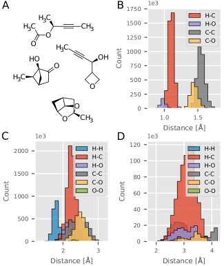
Figure 4: Overview of the Conf17 benchmark. A: Structural formulae of a random selection of molecules. B–D: Distribution of distances (in Å) grouped by edge (B: $E_{\text{bond}}$, C: $E_{\text{angle}}$, and D: $E_{\text{dihedral}}$) and vertex type (chemical element).

5 Experiments

We assess the performance of our method, named Graph Distance Geometry (GraphDG), by comparing it with two state-of-the-art methods for molecular conformation generation: RDKit (Riniker & Landrum, 2015), a classical EDG approach, and DL4Chem (Mansimov et al., 2019), a machine learning approach. We trained GraphDG and DL4Chem on three different training and test splits of the Conf17 benchmark using Adam (Kingma & Ba, 2014). We generated $100$ conformations with each method for molecular graphs in a test set.

5.1 Distributions Over Distances

We assessed the accuracy of the distance distributions of RDKit, DL4Chem, and GraphDG by calculating the maximum mean discrepancy (MMD) (Gretton et al., 2012) to the ground-truth distribution. In particular, we compute the MMD using a Gaussian kernel, where we set the standard deviation to be the median distance between distances $\mathbf{d}$ in the aggregate sample. For this, we determined the distances in the conformations from the ground-truth and those generated by RDKit, DL4Chem, and GraphDG. For each train-test split and each $G$ in a test set, we compute the MMD of the joint distribution of distances between C and O atoms $p(\{d_{k}\}|G)$ (H atoms are usually ignored), the MMDs of pair-wise distances $p(d_{i},d_{j}|G)$, and the MMDs between the marginals of individual distances $p(d_{i}|G)$. We aggregate the results of three train-test splits, and, finally, compute the median MMDs and average rankings. The results are summarized in Table 1. It can be seen that the samples from GraphDG are significantly closer to the ground-truth distribution than the other methods. RDKit is slightly worse than GraphDG while DL4Chem seems to struggle with the complexity of the molecules and the small number of graphs in the training set.

Table 1: Assessment of the accuracy of the distributions over conformations generated by three models compared to the ground-truth. We compare the distributions with respect to the marginals $p(d_{k}|G)$, $p(d_{k},d_{l}|G)$, and the distribution over all edges between C and O atoms $p(\{d_{k}\}|G)$. Two different metrics are used: median MMD between ground-truth conformations and generated ones, and mean ranking (1 to 3) based on the MMD. Reported are the results for molecular graphs in a test set from three train-test splits. Standard deviations are given in brackets.

	Median MMD			Mean Ranking
	RDKit	DL4Chem	GraphDG	RDKit	DL4Chem	GraphDG
$p(d_{k}|G)$	$0.37\;(0.23)$	$1.11\;(0.25)$	$\mathbf{0.13}\;(0.13)$	$1.98\;(0.44)$	$2.90\;(0.35)$	$\textbf{1.12}\;(0.33)$
$p(d_{k},d_{l}|G)$	$0.47\;(0.18)$	$1.12\;(0.15)$	$\mathbf{0.14}\;(0.11)$	$1.95\;(0.29)$	$2.98\;(0.13)$	$\textbf{1.07}\;(0.26)$
$p(\{d_{k}\}|G)$	$0.57\;(0.11)$	$1.03\;(0.13)$	$\mathbf{0.19}\;(0.08)$	$2.00\;(0.00)$	$3.00\;(0.00)$	$\textbf{1.00}\;(0.00)$

In Fig. 5, we showcase the accuracy of our model by plotting the marginal distributions $p(d_{i}|G)$ for distances between C and O atoms, given a molecular graph from a test set. It can be seen that RDKit consistently underestimates the marginal variances. This is because this method aims to predict the most stable conformation, i.e., the distribution’s mode. In contrast, DL4Chem often fails to predict the correct mean. For this molecule, GraphDG is the most accurate, predicting the right mean and variance in most cases. Additional figures can be found in the Appendix, where we also show plots for the marginal distributions $p(d_{i},d_{j}|G)$.

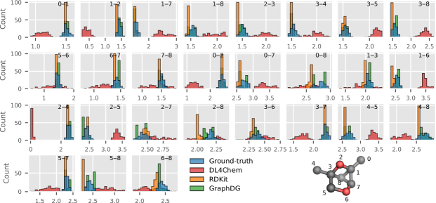
Figure 5: Marginal distributions $p(d_{k}|G)$ of ground-truth and predicted distances (in Å) between C and O atoms given a molecular graph from a test set. The atoms connected by each edge $d_{k}$ are indicated in each subplot ($s_{k}$–$r_{k}$). In the 3D structure of the molecule, carbon and oxygen atoms are colored gray and red, respectively. H atoms are omitted for clarity.

5.2 Generation of Conformations

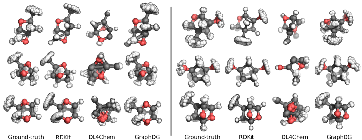
Figure 6: Overlay of 50 conformations from the ground-truth and three models based on six random molecular graphs from the test set. C, O, and H atoms are colored gray, red, and white, respectively.

We passed the distances from our generative model to an EDG algorithm to obtain conformations. For 99.9% of the sets of distances, all triangle inequalities held. For 83% of the molecular graphs, the algorithm succeeded which is 7 pp higher than the success rate we observed for RDKit. For each molecular graph in a test set, we generated 50 conformations with each method. This took DL4Chem, RDKit, and GraphDG on average around hundreds of milliseconds per molecule. In contrast, a single conformation in the ISO17 dataset takes around a minute to compute.

To assess the approximations made in the IS scheme, we studied the overlap between $p(\mathbf{d}|z,\mathcal{G})$ for a given $\mathcal{G}$ and different samples of $z$. We found experimentally that for 50 samples the overlap between the distributions is small. This finding can be explained by the high dimensionality of $\mathbf{d}$ which is on average $\approx 60$.

In Fig. 6, an overlay of these conformations of six molecules generated by the different methods is shown. It can be seen that RDKit’s conformations show too little variance, while DL4Chem’s structures are mostly invalid, which is due in part to its failure to predict the correct interatomic angles. Our method slightly overestimates the structural variance (see, for example, Fig. 6, top row, second column), but produces conformations that are the closest to the ground-truth.

5.3 Calculation of Molecular Properties

We estimate expected molecular properties for molecular graphs from the test set with $N=50$ conformational samples each. Due to their poor quality, we could not compute properties $\mathcal{O}(\mathbf{x})$, including the energy $E(\mathbf{x})$, for conformations generated with DL4Chem, and thus, this method is excluded from this analysis. In Table 2, it can be seen that RDKit and GraphDG perform similarly well (computational details can be found in the Appendix). However, both methods are still highly inaccurate for $E_{\text{elec}}$ (in practice, an accuracy of less than 5 kJ/mol is required). Close inspection of the conformations shows that, even though GraphDG predicts the most accurate distances overall, the variances of certain strongly constrained distances (e.g., triple bonds) are overestimated so that the energies of the conformations increase drastically.

Table 2: Median difference in average properties between ground-truth and RDKit and GraphDG: total electronic energy $E_{\text{elec}}$ (in kJ/mol), the energy of the HOMO and the LUMO $\epsilon_{\text{HOMO}}$ and $\epsilon_{\text{LUMO}}$, respectively (in eV), and the dipole moment $\mu$ (in debye). Reported are the results for molecular graphs from the test set, averaged over three train-test splits. Standard errors are given in brackets.

	RDKit	GraphDG
$E_{\text{elec}}$	$42.7\;(4.3)$	$58.0\;(21.0)$
$\epsilon_{\text{HOMO}}$	$0.08\;(0.04)$	$0.10\;(0.05)$
$\epsilon_{\text{LUMO}}$	$0.15\;(0.03)$	$0.09\;(0.05)$
$\mu$	$0.29\;(0.05)$	$0.33\;(0.09)$

6 Limitations

The first limitation of this work is that the CVAE can sample invalid sets of distances for which there exists no 3D structure. Second, the Conf17 benchmark covers only a small portion of chemical space. Finally, a large set of auxiliary edges would be required to capture long-range correlations (e.g., in proteins). Future work will address these points.

7 Conclusions

We presented GraphDG, a transferable, generative model that allows sampling from a distribution over molecular conformations. We developed a principled learning representation of conformations that is based on distances between atoms. Then, we proposed a challenging benchmark for comparing molecular conformation generators. With this benchmark, we show experimentally that conformations generated by GraphDG are closer to the ground-truth than those generated by other methods. Finally, we employ our model as a proposal distribution in an IS integration scheme to estimate molecular properties. While orbital energies and the dipole moments were predicted well, a larger and more diverse dataset will be necessary for meaningful estimates of electronic energies. Further, methods have to be devised to estimate how many conformations need to be generated to ensure all important conformations have been sampled. Finally, our model could be trained on conformational distributions at different temperatures in a transfer learning-type setting.

Appendix A Conf17 Benchmark

A.1 Data Generation

The ISO17 dataset (Schütt et al., 2017a) was processed in the following way. First, conformations in which could not be parsed by the tool XYZ2Mol (Jensen, 2019) were discarded. Second, the molecular graphs were augmented by adding auxiliary edges for reasons described in the main text. This can lead to an over-specification of the system’s geometry, however, this did not pose a problem in our experiments.

A.2 Input Features

Below we list the node and edge features in the Conf17 benchmark.

Table 3: Node features.

Feature	Data Type	Dimension
atomic number	one-hot (H, He, … F)	9
chiral tag	one-hot (R, S, and None)	3

Table 4: Edge features.

Feature	Data Type	Dimension
kind	one-hot ($E_{\text{bond}}$, $E_{\text{angle}}$, or $E_{\text{dihedral}}$)	3
stereo chemistry	one-hot (E, Z, Any, None)	4
type	one-hot (single, double, triple, aromatic or None)	5
is aromatic	binary	1
is conjugated	binary	1
is in ring of size	one-hot (3, 4, …, 9) or None	7

Appendix B Model Architecture

The source code of the model (including pre-processing scripts) is available online https://github.com/gncs/graphdg. In Table 5, the model architecture are summarized. After each hidden layer, a ReLU non-linearity is used. In Table 6, all hyperparameters are listed.

Table 5: Model architecture for generative model.

Network	Output Layers
$F_{\text{enc},v}$	$50,50,10$
$F_{\text{enc},e}$	$50,50,10$
$\text{MP}^{(t)}_{\text{enc}}$	$50,50,10$
$\text{MP}^{(t)}_{\text{dec}}$	$50,50,10$
$R_{\text{dec},v}$	$50,50,1$
$R_{\text{dec},e}$	$50,50,1$

Table 6: Hyperparameters used throughout this work.

Hyperparameter	Value
Minibatch size	32
Learning rate	0.001
Number of convolutions $T$	3

Appendix C Computational Details

C.1 Quantum-Chemical Calculations

All quantum-chemical calculations were carried out with the PySCF program package (version 1.5) (Sun et al., 2018) employing the exchange-correlation density functional PBE (Perdew et al., 1996), and the def2-SVP (Weigend & Ahlrichs, 2005; Weigend, 2006) basis set.

Conformations generated by DL4Chem did not succeed as some atoms were too close to each other. Self-consistent field algorithms in quantum-chemical software such as PySCF do not converge for such molecular structures.

With quantum-chemical methods, we calculate several properties that concern the states of the electrons in the conformation. These are the total electronic energy $E_{\text{elec}}$, the energy of the electron in the highest occupied molecular orbital (HOMO in eV) $\epsilon_{\text{HOMO}}$, the energy of the lowest unoccupied molecular orbital (LUMO in eV) $\epsilon_{\text{LUMO}}$, and the norm of the dipole moment $\mu$ (in debye).

C.2 Euclidean Distance Geometry

We refer the reader to Havel (2002) for theory on EDG, algorithms, and chemical applications. In summary, the EDG procedure consists of the following three steps:

1. Bound smoothing: extrapolating a complete set of lower and upper limits on all the distances from the sparse set of lower and upper bounds.

2. Embedding: choosing a random distance matrix from within these limits, and computing coordinates that are a certain best-fit to the distances.

3. Optimization: optimizing these coordinates versus an error function which measures the total violation of the distance (and chirality) constraints.

We use the EDG implementation found in RDKit (Riniker & Landrum, 2015) with default settings.

Appendix D Generation of Conformations

Fig. 7 shows an overlay of 50 conformations from the ground-truth, RDKit, DL4Chem, and GraphDG based on two random molecular graphs from a test set.

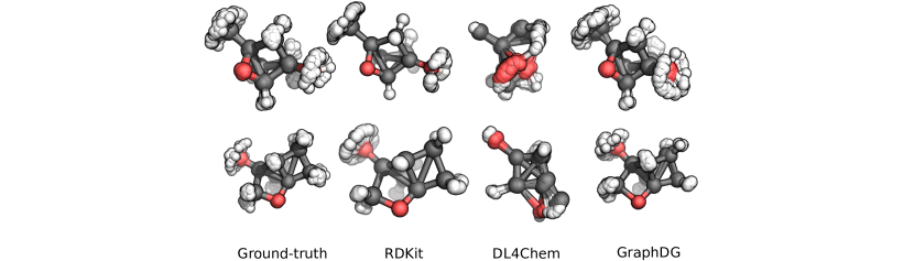
Figure 7: Overlay of 50 conformations from the ground-truth, RDKit, DL4Chem, and GraphDG based on two random molecular graphs from a test set. C, O, and H atoms are colored gray, red, and white, respectively.

Appendix E Distributions over Distances

We show the marginal distributions $p(d_{k}|G)$ and $p(d_{i},d_{j}|G)$ of ground-truth and predicted distances (in Å) for additional molecules from a test set.

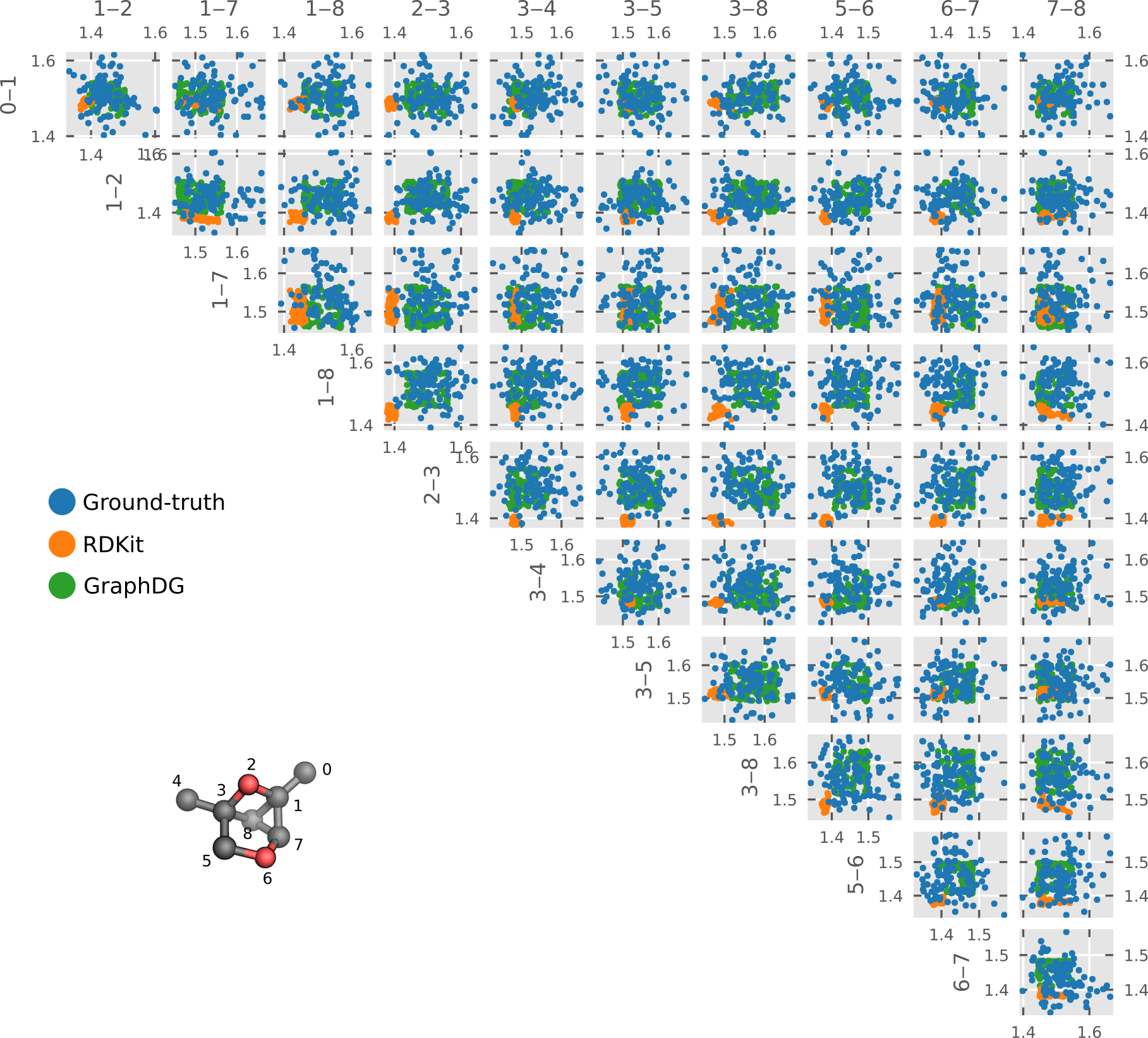
Figure 8: Marginal distributions $p(d_{i},d_{j}|G)$ of ground-truth and predicted distances for a molecular graph from a test set (in Å). Here, $d_{i}$ and $d_{j}$ are restricted to edges representing bonds between C and O atoms. In the 3D structure of the molecule, carbon and oxygen atoms are colored gray and red, respectively. H atoms are omitted for clarity.

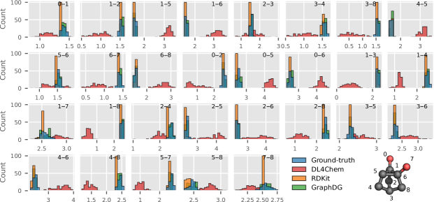
Figure 9: See caption of Fig. 5

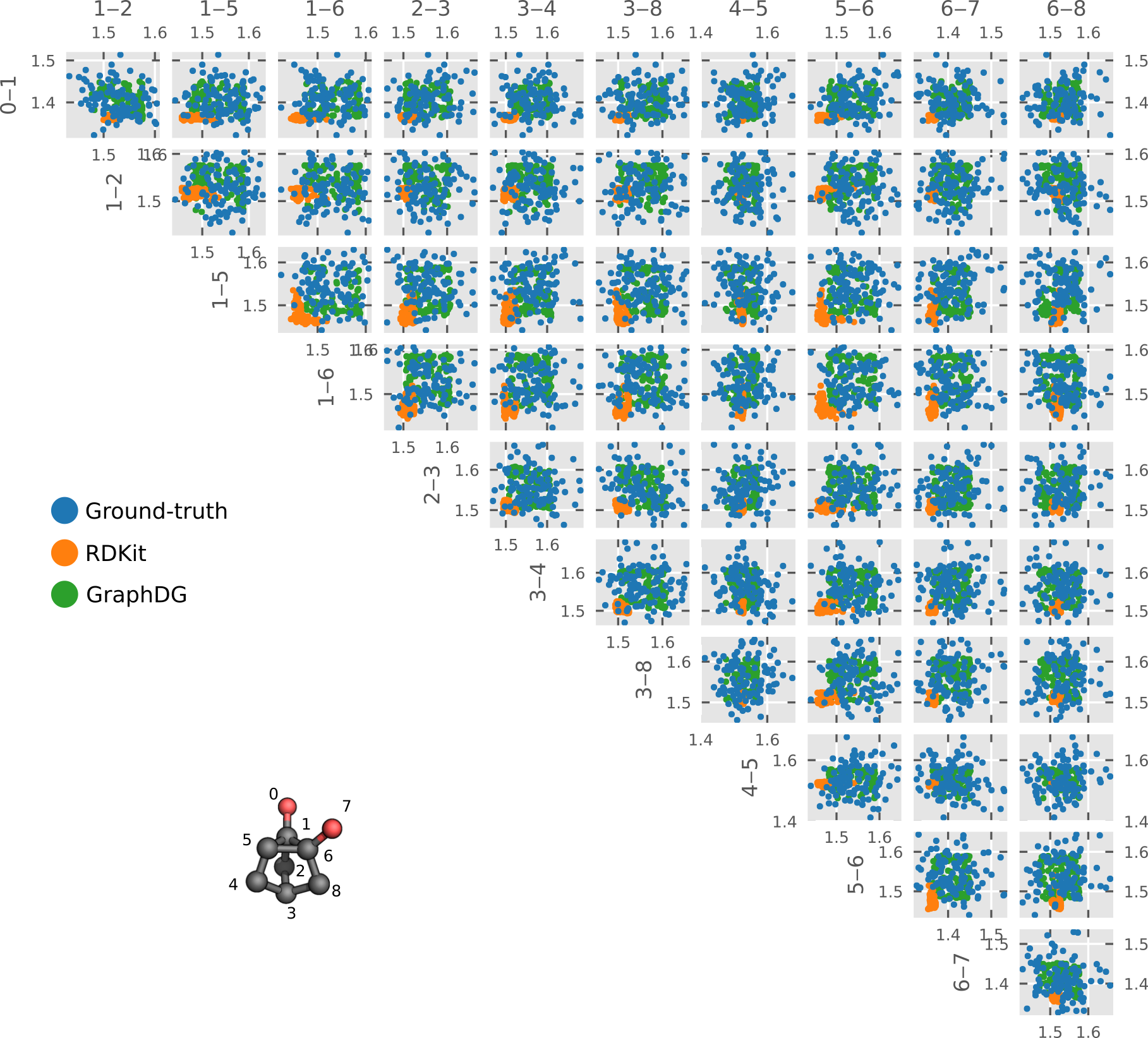
Figure 10: See caption of Fig. 8

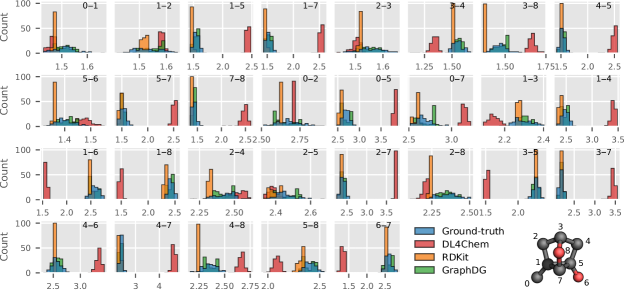
Figure 11: See caption of Fig. 5

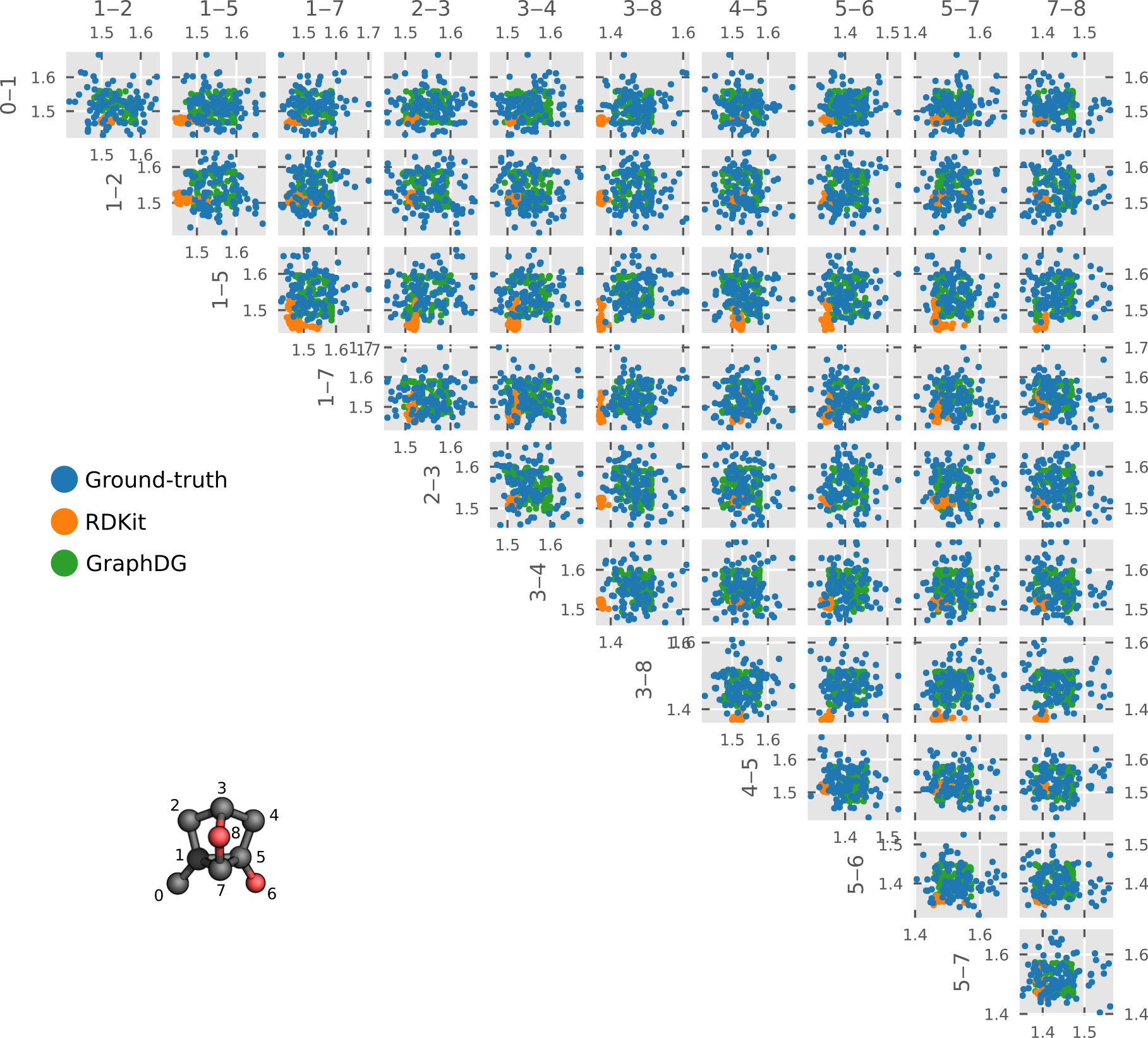
Figure 12: See caption of Fig. 8

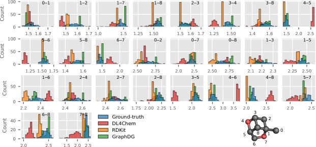
Figure 13: See caption of Fig. 5

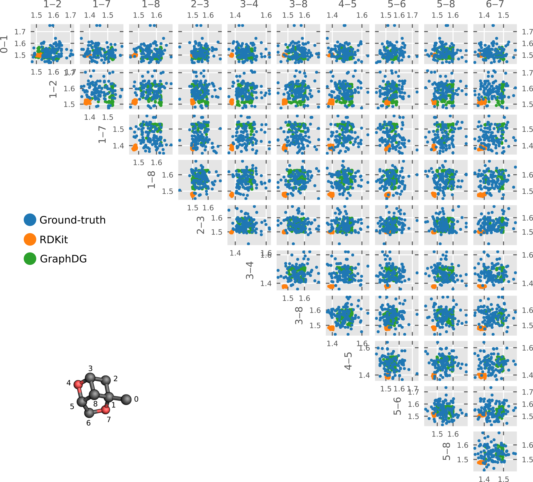
Figure 14: See caption of Fig. 8

References

- Allen (2002) Allen, F. H. The Cambridge Structural Database: A quarter of a million crystal structures and rising. Acta Crystallogr., Sect. B: Struct. Sci, 58(3):380–388, 2002. doi: 10.1107/S0108768102003890.
- AlQuraishi (2019) AlQuraishi, M. End-to-End Differentiable Learning of Protein Structure. Cell Systems, 8(4):292–301.e3, 2019. doi: 10.1016/j.cels.2019.03.006.
- Ballard et al. (2015) Ballard, A. J., Martiniani, S., Stevenson, J. D., Somani, S., and Wales, D. J. Exploiting the potential energy landscape to sample free energy. WIREs Comput. Mol. Sci., 5(3):273–289, 2015. doi: 10.1002/wcms.1217.
- Bishop (2009) Bishop, C. M. Pattern Recognition and Machine Learning. Information Science and Statistics. Springer, New York, 8 edition, 2009. ISBN 978-0-387-31073-2.
- Blaney & Dixon (2007) Blaney, J. M. and Dixon, J. S. Distance Geometry in Molecular Modeling. In Reviews in Computational Chemistry, pp. 299–335. John Wiley & Sons, Ltd, 2007. ISBN 978-0-470-12582-3. doi: 10.1002/9780470125823.ch6.
- Bradshaw et al. (2019a) Bradshaw, J., Kusner, M. J., Paige, B., Segler, M. H. S., and Hernández-Lobato, J. M. A generative model for electron paths. In International Conference on Learning Representations, 2019a.
- Bradshaw et al. (2019b) Bradshaw, J., Paige, B., Kusner, M. J., Segler, M. H. S., and Hernández-Lobato, J. M. A Model to Search for Synthesizable Molecules. arXiv:1906.05221, 2019b.
- Dai et al. (2018) Dai, H., Tian, Y., Dai, B., Skiena, S., and Song, L. Syntax-directed variational autoencoder for structured data. In International Conference on Learning Representations, 2018.
- De Vivo et al. (2016) De Vivo, M., Masetti, M., Bottegoni, G., and Cavalli, A. Role of Molecular Dynamics and Related Methods in Drug Discovery. J. Med. Chem., 59(9):4035–4061, 2016. doi: 10.1021/acs.jmedchem.5b01684.
- Demaine et al. (2009) Demaine, E. D., Gomez-Martin, F., Meijer, H., Rappaport, D., Taslakian, P., Toussaint, G. T., Winograd, T., and Wood, D. R. The distance geometry of music. Computational Geometry, 42(5):429–454, 2009. doi: 10.1016/j.comgeo.2008.04.005.
- Duvenaud et al. (2015) Duvenaud, D. K., Maclaurin, D., Iparraguirre, J., Bombarell, R., Hirzel, T., Aspuru-Guzik, A., and Adams, R. P. Convolutional Networks on Graphs for Learning Molecular Fingerprints. In Cortes, C., Lawrence, N. D., Lee, D. D., Sugiyama, M., and Garnett, R. (eds.), Advances in Neural Information Processing Systems 28, pp. 2224–2232. Curran Associates, Inc., 2015.
- Gilmer et al. (2017) Gilmer, J., Schoenholz, S. S., Riley, P. F., Vinyals, O., and Dahl, G. E. Neural message passing for quantum chemistry. In Proceedings of the 34th International Conference on Machine Learning - Volume 70, ICML’17, pp. 1263–1272, 2017.
- Gómez-Bombarelli et al. (2018) Gómez-Bombarelli, R., Wei, J. N., Duvenaud, D., Hernández-Lobato, J. M., Sánchez-Lengeling, B., Sheberla, D., Aguilera-Iparraguirre, J., Hirzel, T. D., Adams, R. P., and Aspuru-Guzik, A. Automatic Chemical Design Using a Data-Driven Continuous Representation of Molecules. ACS Cent. Sci., 4(2):268–276, 2018. doi: 10.1021/acscentsci.7b00572.
- Gretton et al. (2012) Gretton, A., Borgwardt, K. M., Rasch, M. J., Schölkopf, B., and Smola, A. A Kernel Two-Sample Test. J. Mach. Learn. Res., 13:723–773, 2012.
- Havel (2002) Havel, T. F. Distance Geometry: Theory, Algorithms, and Chemical Applications. In Encyclopedia of Computational Chemistry. American Cancer Society, 2002. ISBN 978-0-470-84501-1. doi: 10.1002/0470845015.cda018.
- Ingraham et al. (2019) Ingraham, J., Riesselman, A., Sander, C., and Marks, D. Learning Protein Structure with a Differentiable Simulator. In International Conference on Learning Representations, 2019.
- Jain & Saul (2004) Jain, V. and Saul, L. K. Exploratory analysis and visualization of speech and music by locally linear embedding. In 2004 IEEE International Conference on Acoustics, Speech, and Signal Processing, volume 3, pp. iii–984, 2004. doi: 10.1109/ICASSP.2004.1326712.
- Jensen (2019) Jensen, J. XYZ2Mol. https://github.com/jensengroup/xyz2mol, 2019.
- Jin et al. (2018) Jin, W., Barzilay, R., and Jaakkola, T. Junction tree variational autoencoder for molecular graph generation. In Dy, J. and Krause, A. (eds.), Proceedings of the 35th International Conference on Machine Learning, volume 80 of Proceedings of Machine Learning Research, pp. 2323–2332, Stockholm, Sweden, 2018. PMLR.
- Kanal et al. (2018) Kanal, I. Y., Keith, J. A., and Hutchison, G. R. A sobering assessment of small-molecule force field methods for low energy conformer predictions. Int. J. Quantum Chem., 118(5):e25512, 2018. doi: 10.1002/qua.25512.
- Kearnes et al. (2016) Kearnes, S., McCloskey, K., Berndl, M., Pande, V., and Riley, P. Molecular graph convolutions: Moving beyond fingerprints. J. Comput.-Aided Mol. Des., 30(8):595–608, 2016. doi: 10.1007/s10822-016-9938-8.
- Kingma & Ba (2014) Kingma, D. P. and Ba, J. Adam: A Method for Stochastic Optimization. arXiv:1412.6980, 2014.
- Kingma & Welling (2014) Kingma, D. P. and Welling, M. Auto-Encoding Variational Bayes. In International Conference on Learning Representations, 2014.
- Kipf & Welling (2017) Kipf, T. N. and Welling, M. Semi-Supervised Classification with Graph Convolutional Networks. International Conference on Learning Representations, 2017.
- Kusner et al. (2017) Kusner, M. J., Paige, B., and Hernández-Lobato, J. M. Grammar Variational Autoencoder. In Precup, D. and Teh, Y. W. (eds.), Proceedings of the 34th International Conference on Machine Learning, volume 70 of Proceedings of Machine Learning Research, pp. 1945–1954, International Convention Centre, Sydney, Australia, 2017. PMLR.
- Lagorce et al. (2009) Lagorce, D., Pencheva, T., Villoutreix, B. O., and Miteva, M. A. DG-AMMOS: A New tool to generate 3D conformation of small molecules using Distance Geometry and Automated Molecular Mechanics Optimization for in silico Screening. BMC Chem. Biol., 9:6, 2009. doi: 10.1186/1472-6769-9-6.
- Lemke & Peter (2019) Lemke, T. and Peter, C. EncoderMap: Dimensionality Reduction and Generation of Molecule Conformations. J. Chem. Theory Comput., 2019. doi: 10.1021/acs.jctc.8b00975.
- Liu et al. (2018) Liu, Q., Allamanis, M., Brockschmidt, M., and Gaunt, A. Constrained Graph Variational Autoencoders for Molecule Design. In Bengio, S., Wallach, H., Larochelle, H., Grauman, K., Cesa-Bianchi, N., and Garnett, R. (eds.), Advances in Neural Information Processing Systems 31, pp. 7795–7804. Curran Associates, Inc., 2018.
- Mansimov et al. (2019) Mansimov, E., Mahmood, O., Kang, S., and Cho, K. Molecular Geometry Prediction using a Deep Generative Graph Neural Network. Sci. Rep., 9(1):1–13, 2019. doi: 10.1038/s41598-019-56773-5.
- Noé et al. (2019) Noé, F., Olsson, S., Köhler, J., and Wu, H. Boltzmann generators: Sampling equilibrium states of many-body systems with deep learning. Science, 365(6457):eaaw1147, 2019. doi: 10.1126/science.aaw1147.
- Pagnoni et al. (2018) Pagnoni, A., Liu, K., and Li, S. Conditional Variational Autoencoder for Neural Machine Translation. arXiv:1812.04405, 2018.
- Perdew et al. (1996) Perdew, J. P., Ernzerhof, M., and Burke, K. Rationale for mixing exact exchange with density functional approximations. J. Chem. Phys., 105(22):9982–9985, 1996. doi: 10.1063/1.472933.
- Ramakrishnan et al. (2014) Ramakrishnan, R., Dral, P. O., Rupp, M., and von Lilienfeld, O. A. Quantum chemistry structures and properties of 134 kilo molecules. Sci. Data, 1:140022, 2014. doi: 10.1038/sdata.2014.22.
- Riniker & Landrum (2015) Riniker, S. and Landrum, G. A. Better Informed Distance Geometry: Using What We Know To Improve Conformation Generation. J. Chem. Inf. Model., 55(12):2562–2574, 2015. doi: 10.1021/acs.jcim.5b00654.
- Schütt et al. (2017a) Schütt, K., Kindermans, P.-J., Sauceda Felix, H. E., Chmiela, S., Tkatchenko, A., and Müller, K.-R. SchNet: A continuous-filter convolutional neural network for modeling quantum interactions. In Guyon, I., Luxburg, U. V., Bengio, S., Wallach, H., Fergus, R., Vishwanathan, S., and Garnett, R. (eds.), Advances in Neural Information Processing Systems 30, pp. 991–1001. Curran Associates, Inc., 2017a.
- Schütt et al. (2017b) Schütt, K. T., Arbabzadah, F., Chmiela, S., Müller, K. R., and Tkatchenko, A. Quantum-chemical insights from deep tensor neural networks. Nat. Commun., 8:13890, 2017b. doi: 10.1038/ncomms13890.
- Segler et al. (2018) Segler, M. H. S., Kogej, T., Tyrchan, C., and Waller, M. P. Generating Focused Molecule Libraries for Drug Discovery with Recurrent Neural Networks. ACS Cent. Sci., 4(1):120–131, 2018. doi: 10.1021/acscentsci.7b00512.
- Senior et al. (2020) Senior, A. W., Evans, R., Jumper, J., Kirkpatrick, J., Sifre, L., Green, T., Qin, C., Žídek, A., Nelson, A. W. R., Bridgland, A., Penedones, H., Petersen, S., Simonyan, K., Crossan, S., Kohli, P., Jones, D. T., Silver, D., Kavukcuoglu, K., and Hassabis, D. Improved protein structure prediction using potentials from deep learning. Nature, pp. 1–5, 2020. doi: 10.1038/s41586-019-1923-7.
- Shim & MacKerell (2011) Shim, J. and MacKerell, Jr., A. D. Computational ligand-based rational design: Role of conformational sampling and force fields in model development. Med. Chem. Commun., 2(5):356–370, 2011. doi: 10.1039/C1MD00044F.
- Sun et al. (2018) Sun, Q., Berkelbach, T. C., Blunt, N. S., Booth, G. H., Guo, S., Li, Z., Liu, J., McClain, J. D., Sayfutyarova, E. R., Sharma, S., Wouters, S., and Chan, G. K.-L. PySCF: The Python-based simulations of chemistry framework. WIREs Comput. Mol. Sci., 8(1), 2018. doi: 10.1002/wcms.1340.
- Tenenbaum et al. (2000) Tenenbaum, J. B., de Silva, V., and Langford, J. C. A Global Geometric Framework for Nonlinear Dimensionality Reduction. Science, 290(5500):2319–2323, 2000. doi: 10.1126/science.290.5500.2319.
- Weigend (2006) Weigend, F. Accurate Coulomb-fitting basis sets for H to Rn. Phys. Chem. Chem. Phys., 8(9):1057–1065, 2006. doi: 10.1039/B515623H.
- Weigend & Ahlrichs (2005) Weigend, F. and Ahlrichs, R. Balanced basis sets of split valence, triple zeta valence and quadruple zeta valence quality for H to Rn: Design and assessment of accuracy. Phys. Chem. Chem. Phys., 7(18):3297–3305, 2005. doi: 10.1039/B508541A.
- Weinberger & Saul (2006) Weinberger, K. Q. and Saul, L. K. Unsupervised Learning of Image Manifolds by Semidefinite Programming. Int. J. Comput. Vision, 70(1):77–90, 2006. doi: 10.1007/s11263-005-4939-z.
- You et al. (2018) You, J., Liu, B., Ying, Z., Pande, V., and Leskovec, J. Graph Convolutional Policy Network for Goal-Directed Molecular Graph Generation. In Bengio, S., Wallach, H., Larochelle, H., Grauman, K., Cesa-Bianchi, N., and Garnett, R. (eds.), Advances in Neural Information Processing Systems 31, pp. 6410–6421. Curran Associates, Inc., 2018.