Online Non-Monotone DR-Submodular Maximization

Abstract

In this paper, we study fundamental problems of maximizing DR-submodular continuous functions that have real-world applications in the domain of machine learning, economics, operations research and communication systems. It captures a subclass of non-convex optimization that provides both theoretical and practical guarantees. Here, we focus on minimizing regret for online arriving non-monotone DR-submodular functions over different types of convex sets: hypercube, down-closed and general convex sets.

First, we present an online algorithm that achieves a $1/e$-approximation ratio with the regret of $O(T^{2/3})$ for maximizing DR-submodular functions over any down-closed convex set. Note that, the approximation ratio of $1/e$ matches the best-known guarantee for the offline version of the problem. Moreover, when the convex set is the hypercube, we propose a tight 1/2-approximation algorithm with regret bound of $O(\sqrt{T})$. Next, we give an online algorithm that achieves an approximation guarantee (depending on the search space) for the problem of maximizing non-monotone continuous DR-submodular functions over a general convex set (not necessarily down-closed). To best of our knowledge, no prior algorithm with approximation guarantee was known for non-monotone DR-submodular maximization in the online setting. Finally we run experiments to verify the performance of our algorithms on problems arising in machine learning domain with the real-world datasets.

1 Introduction

Continuous DR-submodular optimization is a subclass of non-convex optimization that is an upcoming frontier in machine learning. Roughly speaking, a differentiable non-negative bounded function $F\mathrel{\mathop{\mathchar 58\relax}}[0,1]^{n}\rightarrow[0,1]$ is DR-submodular if $\nabla F(\bm{x})\geq\nabla F(\bm{y})$ for all $\bm{x},\bm{y}\in[0,1]^{n}$ where $x_{i}\leq y_{i}$ for every $1\leq i\leq n$. (Note that, w.l.o.g. after normalization, assume that $F$ has values in $[0,1]$.) Intuitively, continuous DR-submodular functions represent the diminishing returns property or the economy of scale in continuous domains. DR-submodularity has been of great interest [3, 1, 10, 21, 29, 33]. Many problems arising in machine learning and statistics, such as Non-definite Quadratic Programming [23], Determinantal Point Processes [25], log-submodular models [12], to name a few, have been modelled using the notion of continuous DR-submodular functions.

In the past decade, online computational framework has been quite successful for tackling a wide variety of challenging problems and capturing many real-world problems with uncertainty. In this computational framework, we focus on the model of online learning. In online learning, at any time step, given a history of actions and a set of associated reward functions, online algorithm first chooses an action from a set of feasible actions; then, an adversary subsequently selects a reward function. The objective is to perform as good as the best fixed action in hindsight. This setting have been extensively explored in the literature, especially in context of convex functions [22].

In fact, several algorithms with theoretical approximation guarantees are known for maximizing (offline and online) DR-submodular functions. However, these guarantees hold under the assumptions that are based on the monotonicity of functions coupled with the structure of convex sets such as unconstrained hypercube and down-closed. Though, a majority of real-world problems can be formulated as non-monotone DR-submodular functions over convex sets that might not be necessarily down-closed. For example, the problems of Determinantal Point Processes, log-submodular models, etc can be viewed as non-monotone DR-submodular maximization problems. Besides, general convex sets include conic convex sets, up-closed convex sets, mixture of covering and packing linear constraints, etc. which appear in many applications. Among others, conic convex sets play a crucial role in convex optimization. Conic programming [4] — an important subfield of convex optimization — consists of optimizing an objective function over a conic convex set. Conic programming reduces to linear programming and semi-definite programming when the objective function is linear and the convex cones are the positive orthant $\mathbb{R}^{n}_{+}$ and positive semidefinite matrices $\mathbb{S}^{n}_{+}$, respectively. Optimizing non-monotone DR-submodular functions over a (bounded) conic convex set (not necessarily downward-closed) is an interesting and important problem both in theory and in practice. To best of our knowledge, no prior work has been done on maximizing DR-submodular functions over conic sets in online setting. The limit of current theory [3, 1, 10, 21, 29, 36] motivates us to develop online algorithms for non-monotone functions.

In this work, we explore the online problem of maximizing non-monotone DR-submodular functions over a hypercube, down-closed and over a general convex sets. Formally, we consider the following setting for DR-submodular maximization: given a convex domain $\mathcal{K}\subseteq[0,1]^{n}$ in advance, at each time step $t=1,2,\ldots,T$, the online algorithm first selects a vector $\bm{x}^{t}\in\mathcal{K}$. Subsequently, the adversary reveals a non-monotone continuous DR-submodular function $F^{t}$ and the algorithm receives a reward of $F^{t}(\bm{x}^{t})$. The objective is also to maximize the total reward. We say that an algorithm achieves a $(r,R(T))$-regret if

$$\sum_{t=1}^{T}F^{t}(\bm{x}^{t}) \geq r\cdot\max_{\bm{x}\in\cal K}\sum_{t=1}^{T}F^{t}(\bm{x})-R(T)$$

In other words, $r$ is the approximation ratio that measures the quality of the online algorithm compared to the best fixed solution in hindsight and $R(T)$ represents the regret in the classic terms. Equivalently, we say that the algorithm has $r$-regret at most $R(T)$. Our goal is to design online algorithms with $(r,R(T))$-regret where $0<r\leq 1$ is as large as possible, and $R(T)$ is sub-linear in $T$, i.e., $R(T)=o(T)$.

1.1 Our contributions and techniques

In this paper, we provide algorithms with performance guarantees for the problem over the hypercube $[0,1]^{n}$, over down-closed and general convex sets. Our contributions and techniques are summarized as follows (also see Table 1, the entries in the red correspond to our contribution).

		Monotone	Non-monotone
Offline	hypercube		$\frac{1}{2}$-approx [3, 29]
	down-closed	$\left(1-\frac{1}{e}\right)$-approx [2]	$\left(\frac{1}{e}\right)$-approx [1]
	general	$\left(1-\frac{1}{e}\right)$-approx [28]	$\left(\frac{1-\min_{\bm{x}\in\mathcal{K}}\|\bm{x}\|_{\infty}}{3\sqrt{3}}\right)$-approx [14]
Online	hypercube		$\left(1/2,O\bigl{(}\sqrt{T}\bigr{)}\right)$
	down-closed		$\left(\frac{1}{e},O\bigl{(}T^{2/3}\bigr{)}\right)$
	general	$\left(1-\frac{1}{e},O\bigl{(}\sqrt{T}\bigr{)}\right)$ [10]	$\left(\frac{1-\min_{\bm{x}\in\mathcal{K}}\|\bm{x}\|_{\infty}}{3\sqrt{3}},O\bigl{(}\frac{T}{\ln T}\bigr{)}\right)$

Table 1: Summary of results on DR-submodular maximization. The entries represent the best-known $(r,R(T))$-regret; our results are shown in red. The guarantees in blank cells can be deduced from a more general one.

1.1.1 Maximizing online non-monotone DR-submodular functions over down-closed convex sets

We present an online algorithm that achieves $\bigl{(}1/e,O(T^{2/3})\bigr{)}$-regret in expectation where $T$ is number of time steps. Our algorithm is inspired by the Meta-Frank-Wolfe algorithm introduced by Chen et al. [10] for monotone DR-submodular maximization. Their meta Frank-Wolfe algorithm combines the framework of meta-actions proposed in [34] with a variant of the Frank-Wolfe proposed in [2] for maximizing monotone DR-submodular functions. Informally, at every time $t$, our algorithm starts from the origin $\bm{0}$ ($\bm{0}\in\mathcal{K}$ since $\mathcal{K}$ is down-closed) and executes $L$ steps of the Frank-Wolfe algorithm where every update vector at iteration $1\leq\ell\leq L$ is constructed by combining the output of an optimization oracle $\mathcal{E}_{\ell}$ and the current vector so that we can exploit the concavity property in positive directions of DR-submodular functions. The solution $\bm{x}^{t}$ is produced at the end of the $L$-th step. Subsequently, after observing the function $F^{t}$, the algorithm subtly defines a vector $\bm{d}^{t}_{\ell}$ and feedbacks $\langle\cdot,\bm{d}^{t}_{\ell}\rangle$ as the reward function at time $t$ to the oracle $\mathcal{E}_{\ell}$ for $1\leq\ell\leq L$. The most important distinguishing point of our algorithm compared to that in [10] relies on the oracles. In their algorithm, they used linear oracles which are appropriate for maximizing monotone DR-submodular functions. However, it is not clear whether linear or even convex oracles are strong enough to achieve a constant approximation for non-monotone functions.

While aiming for a $1/e$-approximation — the best known approximation in the offline setting — we consider the following online non-convex problem, referred throughout this paper as online vee learning problem. At each time $t$, the online algorithm knows $\bm{c}^{t}\in\mathcal{K}$ in advance and selects a vector $\bm{x}^{t}\in\mathcal{K}$. Subsequently, the adversary reveals a vector $\bm{a}^{t}\in\mathbb{R}^{n}$ and the algorithm receives a reward $\langle\bm{a}^{t},\bm{c}^{t}\vee\bm{x}^{t}\rangle$. Given two vectors $\bm{x}$ and $\bm{y}$, the vector $\bm{x}\vee\bm{y}$ has the $i^{th}$ coordinate $(x\vee y)_{i}=\max\{x(i),y(i)\}$. The goal is to maximize the total reward over a time horizon $T$.

In order to bypass the non-convexity of the online vee learning problem, we propose the following methodology. Unlike dimension reduction techniques that aim at reducing the dimension of the search space, we lift the search space and the functions to a higher dimension so as to benefit from their properties in this new space. Concretely, at a high level, given a convex set $\mathcal{K}$, we define a “sufficiently dense” lattice $\mathcal{L}$ in $[0,1]^{n}$ such that every point in $\mathcal{K}$ can be approximated by a point in the lattice. The term “sufficiently dense” corresponds to the fact that the values of any Lipschitz function can be approximated by the function values at lattice points. As the next step, we lift all lattice points in $\mathcal{K}$ to a high dimension space so that they form a subset of vertices (corners points) $\widetilde{\mathcal{K}}$ of the unit hypercube in the newly defined space. Interestingly, the reward function $\langle\bm{a}^{t},\bm{c}^{t}\vee\bm{x}^{t}\rangle$ can be transformed to a linear function in the new space. Hence, our algorithm for the online vee problem consists of updating at every time step a solution in the high-dimension space using a linear oracle and projecting the solution back to the original space.

Once the solution is projected back to original space, we construct appropriate update vectors for the original DR-submodular maximization and feedback rewards for the online vee oracle. Exploiting the underlying properties of DR-submodularity, we show that our algorithm achieves the regret bound of $(1/e,O(T^{2/3}))$.

1.1.2 Maximizing online non-monotone DR-submodular functions over the hypercube

Next, we consider a particular down-closed convex set, the hypercube $[0,1]^{n}$, that has been widely studied in the context of submodular maximization. In offline setting, several algorithms with tight approximation guarantee of $1/2$ are known [3, 29]; however it is not clear how to extend those algorithms to the online setting. Besides, in the context of discrete setting, Roughgarden and Wang [30] recently gave 1/2-approximation algorithm for the problem of maximizing online (discrete) submodular functions. In the light of this, an intriguing open question is that if one can achieve $1/2$-approximation for DR-submodular maximization in the continuous setting. Note that several properties used for achieving $1/2$-approximation solutions in the discrete setting or in the offline continuous setting do not necessarily hold in the online settings.

Building upon our salient ideas from previous algorithm, we present an online algorithm that achieves $1/2$-approximation for DR-submodular maxmization over the hypercube. Essentially, we reduce the DR-submodular maximization over $[0,1]^{n}$ to the problem of maximizing discrete submodular functions over vertices of the hypercube in a higher dimensional space. We do it also by lifting points of a lattice in $[0,1]^{n}$ to vertices in $\{0,1\}^{n\times\log T}$ and prove that this operation transforms DR-submodular functions to submodular set-functions. Applying algorithm of [30] and performing an independent rounding, we provide an algorithm with the tight approximation ratio of $1/2$ while maintaining the $1/2$-regret bound of $O(\sqrt{T})$.

1.1.3 Maximizing online non-monotone DR-submodular functions over general convex sets

For general convex sets, we prove that the Meta-Frank-Wolfe algorithm with adapted step-sizes guarantees $\left(\frac{1-\min_{\bm{x}\in\mathcal{K}}\|\bm{x}\|_{\infty}}{3\sqrt{3}},O\bigl{(}\frac{T}{\ln T}\bigr{)}\right)$-regret in expectation. Notably, if the domain $\cal K$ contains $\bm{0}$ (as in the case where $\cal K$ is the intersection of a cone and the hypercube $[0,1]^{n}$) then the algorithm guarantees in expectation a $\bigl{(}\frac{1}{3\sqrt{3}},O\bigl{(}\frac{T}{\log T}\bigr{)}\bigr{)}$-regret. To the best of our knowledge, this is the first constant-approximation algorithm for the problem of online non-monotone DR-submodular maximization over a non-trivial convex set that goes beyond down-closed sets. Remark that the quality of the solution, specifically the approximation ratio, depends on the initial solution $\bm{x}_{0}$. This confirms an observation in various contexts that initialization plays an important role in non-convex optimization.

1.2 Related Work

In this section, we give a summary on best-known results on DR-submodular maximization. The domain has been investigated more extensively in recent years due to its numerous applications in the field of statistics and machine learning, for example active learning [18], viral makerting [24], network monitoring [19], document summarization [26], crowd teaching [31], feature selection [16], deep neural networks [15], diversity models [13] and recommender systems [20].

Offline setting.

Bian et al. [2] considered the problem of maximizing monotone DR-functions subject to a down-closed convex set and showed that the greedy method proposed by [7], a variant of well-known Frank-Wolfe algorithm in convex optimization, guarantees a $(1-1/e)$-approximation. However, it has been observed by [21] that the greedy method is not robust in stochastic settings (where only unbiased estimates of gradients are available). Subsequently, Hassani et al. [28] proposed a $(1-1/e)$-approximation algorithm for maximizing monotone DR-submodular functions over general convex sets in stochastic settings by a new variance reduction technique.

The problem of maximizing non-monotone DR-submodular functions is much harder. Bian et al. [3] and Niazadeh et al. [29] have independently presented algorithms with the same approximation guarantee of $(1/2)$ for the problem of non-monotone DR-submodular maximization over the hypercube ($\mathcal{K}=[0,1]^{n}$). These algorithms are inspired by the bi-greedy algorithms in [6, 5]. Bian et al. [1] made a further step by providing a $(1/e)$-approximation algorithm where the convex sets are down-closed. Mokhtari et al. [28] also presented an algorithm that achieve $(1/e)$ for non-monotone continuous DR-submodular function over a down-closed convex domain that uses only stochastic gradient estimates. Remark that when aiming for approximation algorithms (in polynomial time), the restriction to down-closed polytopes is unavoidable. Specifically, Vondrak [35] proved that any algorithm for the problem over a non-down-closed set that guarantees a constant approximation must require in general exponentially many value queries to the function. Recently, Durr et al. [14] presented an algorithm that achieves $\bigl{(}(1-\min_{\bm{x}\in\mathcal{K}}\|\bm{x}\|_{\infty})/3\sqrt{3}\bigr{)}$-approximation for non-monotone DR-submodular function over general convex sets that are not necessarily down-closed.

Online setting.

The results for online DR-submodular maximization are known only for monotone functions. Chen et al. [10] considered the online problem of maximizing monotone DR-submodular functions over general convex sets and provided an algorithm that achieves a $\bigl{(}1-1/e,O(\sqrt{T})\bigr{)}$-regret. Subsequently, Zhang et al. [36] presented an algorithm that reduces the number of per-function gradient evaluations from $T^{3/2}$ in [10] to $1$ and achieves the same approximation ratio of $(1-1/e)$. Leveraging the idea of one gradient per iteration, they presented a bandit algorithm for maximizing monotone DR-submodular function over a general convex set that achieves in expectation $(1-1/e)$ approximation ratio with regret $O(T^{8/9})$. Note that in the discrete setting, [30] studied the non-monotone (discrete) submodular maximization over the hypercube and gave an algorithm which guarantees the tight $(1/2)$-approximation and $O(\sqrt{T})$ regret.

2 Preliminaries and Notations

Throughout the paper, we use bold face letters, e.g., $\bm{x},\bm{y}$ to represent vectors. For every $S\subseteq\{1,2,\ldots,n\}$, vector $\bm{1}_{S}$ is the $n$-dim vector whose $i^{th}$ coordinate equals to 1 if $i\in S$ and $0$ otherwise. Given two $n$-dimensional vectors $\bm{x},\bm{y}$, we say that $\bm{x}\leq\bm{y}$ iff $x_{i}\leq y_{i}$ for all $1\leq i\leq n$. Additionally, we denote by $\bm{x}\vee\bm{y}$, their coordinate-wise maximum vector such that $(x\vee y)_{i}=\max\{x_{i},y_{i}\}$. Moreover, the symbol $\circ$ represents the element-wise multiplication that is, given two vectors $\bm{x},\bm{y}$, vector $\bm{x}\circ\bm{y}$ is the such that the $i$-th coordinate $(\bm{x}\circ\bm{y})_{i}=x_{i}y_{i}$. The scalar product $\langle\bm{x},\bm{y}\rangle=\sum_{i}x_{i}y_{i}$ and the norm $\|\bm{x}\|=\langle\bm{x},\bm{x}\rangle^{1/2}$. In the paper, we assume that $\mathcal{K}\subseteq[0,1]^{n}$. We say that $\mathcal{K}$ is the hypercube if $\mathcal{K}=[0,1]^{n}$; $\mathcal{K}$ is down-closed if for every $\bm{z}\in\mathcal{K}$ and $\bm{y}\leq\bm{z}$ then $\bm{y}\in\mathcal{K}$; and $\mathcal{K}$ is general if $\mathcal{K}$ is a convex subset of $[0,1]^{n}$ without any special property.

Definition 1.

A function $F\mathrel{\mathop{\mathchar 58\relax}}[0,1]^{n}\rightarrow\mathbb{R}^{+}\cup\{0\}$ is diminishing-return (DR) submodular if for all vector $\bm{x}\geq\bm{y}\in[0,1]^{n}$, any basis vector $\bm{e}_{i}=(0,\ldots,0,1,0,\ldots,0)$ and any constant $\alpha>0$ such that $\bm{x}+\alpha\bm{e}_{i}\in[0,1]^{n}$, $\bm{y}+\alpha\bm{e}_{i}\in[0,1]^{n}$, it holds that

$$F(\bm{x}+\alpha\bm{e}_{i})-F(\bm{x})\leq F(\bm{y}+\alpha\bm{e}_{i})-F(\bm{y}).$$ (1)

Note that if function $F$ is differentiable then the diminishing-return (DR) property (1) is equivalent to

$$\nabla F(\bm{x})\leq\nabla F(\bm{y})\qquad\forall\bm{x}\geq\bm{y}\in[0,1]^{n}.$$ (2)

Moreover, if $F$ is twice-differentiable then the DR property is equivalent to all of the entries of its Hessian being non-positive, i.e., $\frac{\partial^{2}F}{\partial x_{i}\partial x_{j}}\leq 0$ for all $1\leq i,j\leq n$.

Besides, a differentiable function $F\mathrel{\mathop{\mathchar 58\relax}}\mathcal{K}\subseteq[0,1]^{n}\rightarrow\mathbb{R}^{+}\cup\{0\}$ is said to be $\beta$-smooth if for any $\bm{x},\bm{y}\in\mathcal{K}$, the following holds,

$$F(\bm{y})\leq F(\bm{x})+\langle\nabla F(\bm{x}),\bm{y}-\bm{x}\rangle+\frac{\beta}{2}\|\bm{y}-\bm{x}\|^{2}$$ (3)

or equivalently, the gradient is $\beta$-Lipschitz, i.e.,

$$\mathinner{\!\left\lVert\nabla F(\bm{x})-\nabla F(\bm{y})\right\rVert}\leq\beta\mathinner{\!\left\lVert\bm{x}-\bm{y}\right\rVert}.$$ (4)

Properties of DR-submodularity

In the following, we present a property of DR-submodular functions that are are crucial in our analyses. The most important property is the concavity in positive directions, i.e., for every $\bm{x},\bm{y}\in\mathcal{K}$ and $\bm{x}\geq\bm{y}$, it holds that

$$F(\bm{x})\leq F(\bm{y})+\langle\nabla F(\bm{y}),\bm{x}-\bm{y}\rangle.$$

Addionally, the following lemmas are useful in our analysis.

Lemma 1 ([21]).

For every $\bm{x},\bm{y}\in\mathcal{K}$ and any DR-submodular function $F$, it holds that

$$\langle\nabla F(\bm{x}),\bm{y}-\bm{x}\rangle\geq F(\bm{x}\vee\bm{y})+F(\bm{x}\wedge\bm{y})-2F(\bm{x})$$

Lemma 2 ([17, 8, 1]).

For every $\bm{x},\bm{y}\in\mathcal{K}$ and for any DR-submodular function $F\mathrel{\mathop{\mathchar 58\relax}}[0,1]^{n}\rightarrow\mathbb{R}^{+}\cup\{0\}$, it holds that $F(\bm{x}\vee\bm{y})\geq\bigl{(}1-\|\bm{x}\|_{\infty}\bigr{)}F(\bm{y})$.

Variance Reduction Technique.

Our algorithm and its analysis relies on a recent variance reduction technique proposed by [28]. This theorem has also been used in the context of online monotone submodular maximization [9, 36].

Lemma 3 ([28], Lemma 2).

Let $\{\bm{a}^{t}\}_{t=0}^{T}$ be a sequence of points in $\mathbb{R}^{n}$. such that $\mathinner{\!\left\lVert\bm{a}^{t}-\bm{a}^{t-1}\right\rVert}\leq C/(t+s)$ for all $1\leq t\leq T$ with fixed constants $C\geq 0$ and $s\geq 3$. Let $\{\tilde{\bm{a}}\}_{t=1}^{T}$ be a sequence of random variables such that $\mathbb{E}[\tilde{\bm{a}}|\mathcal{H}^{t-1}]=\bm{a}^{t}$ and $\mathbb{E}\left[\mathinner{\!\left\lVert\tilde{\bm{a}}^{t}-\bm{a}^{t}\right\rVert}^{2}|\mathcal{H}^{t-1}\right]\leq\sigma^{2}$ for every $t\geq 0$, where $\mathcal{H}^{t-1}$ is the history up to $t-1$. Let $\{\bm{d}^{t}\}_{t=0}^{T}$ be a sequence of random variables where $\bm{d}^{0}$ is fixed and subsequent $\bm{d}^{t}$ are obtained by the recurrence

$$\bm{d}^{t}=(1-\rho^{t})\bm{d}^{t-1}+\rho^{t}\tilde{\bm{a}}^{t}$$

with $\rho^{t}=\frac{2}{(t+s)^{2/3}}$. Then we have

$$\mathbb{E}\left[\mathinner{\!\left\lVert\bm{a}^{t}-\bm{d}^{t}\right\rVert}^{2}\right]\leq\frac{Q}{(t+s+1)^{2/3}},$$

where $Q=\max\{\mathinner{\!\left\lVert\bm{a}^{0}-\bm{d}^{0}\right\rVert}^{2}(s+1)^{2/3},4\sigma^{2}+3C^{2}/2\}$.

3 Online DR-Submodular Maximization over Down-Closed Convex Sets

3.1 Online Vee Learning

In this section, we give an algorithm for an online problem that will be the main building block in the design of algorithms for online DR-submodular maximization over down-closed convex sets. In the online vee learning problem, given a down-closed convex set $\mathcal{K}$, at every time $t$, the online algorithm receives $\bm{c}^{t}\in{\cal K}$ at the beginning of the step and needs to choose a vector $\bm{x}^{t}\in\mathcal{K}$. Subsequently, the adversary reveals a vector $\bm{a}^{t}\in\mathbb{R}^{n}$ and the algorithm receives a reward $\langle\bm{a}^{t},\bm{c}^{t}\vee\bm{x}^{t}\rangle$. The goal is to maximize the total reward $\sum_{t=1}^{T}\langle\bm{a}^{t},\bm{c}^{t}\vee\bm{x}^{t}\rangle$ over a time horizon $T$.

The main issue in the online vee problem is that the reward functions are non-concave. In order to overcome this obstacle, we consider a novel approach that consists of discretizing and lifting the corresponding functons to a higher dimensional space.

Discretization and lifting.

Let $\mathcal{L}$ be a lattice such that $\mathcal{L}=\{0,\frac{1}{M},\frac{2}{M},\ldots,\frac{\ell}{M},\ldots,1\}^{n}$ where $0\leq\ell\leq M$ for some parameter $M$ (to be defined later). Note that each $x_{i}=\frac{\ell}{M}$ for $1\leq\ell\leq M$ can be uniquely represented by a vector $\bm{y}_{i}\in\{0,1\}^{M}$ such that $y_{i1}=\ldots=y_{i\ell}=1$ and $y_{i,\ell+1}=\ldots=y_{i,M}=0$. Based on this observation, we lift the discrete set $\mathcal{K}\cap\mathcal{L}$ to the $(n\times M)$-dim space. Specifically, define a lifting map $m\mathrel{\mathop{\mathchar 58\relax}}\mathcal{K}\cap\mathcal{L}\rightarrow\{0,1\}^{n\times M}$ such that each point $(x_{1},\ldots,x_{n})\in\mathcal{K}\cap\mathcal{L}$ is mapped to an unique point $(y_{10},\ldots,y_{1M},\ldots,y_{n0},\ldots,y_{nM})\in\{0,1\}^{n\times M}$ where $y_{i1}=\ldots=y_{i\ell}=1$ and $y_{i,\ell+1}=\ldots=y_{i,M}=0$ iff $x_{i}=\frac{\ell}{M}$ for $1\leq\ell\leq M$. Define $\widetilde{\mathcal{K}}$ be the set $\{\bm{1}_{X}\in\{0,1\}^{n\times M}\mathrel{\mathop{\mathchar 58\relax}}\bm{1}_{X}=m(\bm{x})\text{ for some }\bm{x}\in\mathcal{K}\cap\mathcal{L}\}$. Observe that $\widetilde{\mathcal{K}}$ is a subset of discrete points in $\{0,1\}^{n\times M}$. Let $\mathcal{C}\mathrel{\mathop{\mathchar 58\relax}}=\texttt{conv}(\widetilde{\mathcal{K}})$ be the convex hull of $\widetilde{\mathcal{K}}$.

Algorithm description.

In our algorithm, at every time $t$, we will output $\bm{x}^{t}\in\mathcal{L}\cap\mathcal{K}$. In fact, we will reduce the online vee problem to a online linear optimization problem in the $(n\times M)$-dim space. Given $\bm{c}^{t}\in{\cal K}$, we round every coordinate $c^{t}_{i}$ for $1\leq i\leq n$ to the largest multiple of $\frac{1}{M}$ which is smaller than $c^{t}_{i}$. In other words, the rounded vector $\overline{\bm{c}}^{t}$ has the $i^{th}$-coordinate $\bar{c}^{t}_{i}=\frac{\ell}{M}$ where $\frac{\ell}{M}\leq c^{t}_{i}<\frac{\ell+1}{M}$. Vector $\overline{\bm{c}}^{t}\in\mathcal{L}$ and also $\overline{\bm{c}}^{t}\in\mathcal{K}$ (since $\overline{\bm{c}}^{t}\leq\bm{c}^{t}$ and $\mathcal{K}$ is down-closed). Denote $\bm{1}_{C^{t}}=m(\overline{\bm{c}}^{t})$. Besides, for each vector $\bm{a}^{t}\in\mathbb{R}^{n}$, define its correspondence $\widetilde{\bm{a}}^{t}\in\mathbb{R}^{n\times M}$ such that $\widetilde{a}^{t}_{i,j}=\frac{1}{M}a^{t}_{i}$ for all $1\leq i\leq n$ and $1\leq j\leq M$. Observe that $\langle\bm{a}^{t},\overline{\bm{c}}^{t}\rangle=\langle\widetilde{\bm{a}}^{t},\bm{1}_{C^{t}}\rangle$ (where the second scalar product is taken in the space of dimension $n\times M$).

Input: A convex set $\mathcal{K}$, a time horizon $T$.

1:  Let $\mathcal{L}$ be a lattice in $[0,1]^{n}$ and denote the polytope $\mathcal{C}\mathrel{\mathop{\mathchar 58\relax}}=\texttt{conv}(\widetilde{\mathcal{K}})$.

2:  Initialize arbitrarily $\bm{x}^{1}\in\mathcal{K}\cap\mathcal{L}$ and $\bm{y}^{1}=\bm{1}_{X^{1}}=m(\bm{x}^{1})\in\widetilde{\mathcal{K}}$.

3:  for $t=1$ to $T$ do

4:     Observe $\bm{c}^{t}$, compute $\bm{1}_{C^{t}}=m(\overline{\bm{c}}^{t})$.

5:     Play $\bm{x}^{t}$.

6:     Observe $\bm{a}^{t}$ (so compute $\widetilde{\bm{a}}^{t}$) and receive the reward $\langle\bm{a}^{t},\bm{x}^{t}\rangle$.

7:     Set $\bm{y}^{t+1}\leftarrow\texttt{update}_{\mathcal{C}}(\bm{y}^{t};\widetilde{\bm{a}}^{t^{\prime}}\circ(\bm{1}-\bm{1}_{C^{t^{\prime}}})\mathrel{\mathop{\mathchar 58\relax}}t^{\prime}\leq t)$ where $\circ$ denotes the element-wise multiplication.

8:     Round: $\bm{1}_{X^{t+1}}\leftarrow\texttt{round}(\bm{y}^{t+1})$.

9:     Compute $\bm{x}^{t+1}=m^{-1}(\bm{1}_{X^{t+1}})$.

10:  end for

Algorithm 1 Online algorithm for vee learning

The formal description is given in Algorithm 1. In the algorithm, we use a procedure update. This procedure takes arguments as the polytope $\mathcal{C}$, the current vector $\bm{y}^{t}$, the gradients of previous time steps $\widetilde{\bm{a}}^{t}\circ(\bm{1}-\bm{1}_{C^{t}})$ and outputs the next vector $\bm{y}^{t+1}$. One can use different update strategies, in particular the gradient descent or the follow-the-perturbed-leader algorithm (if aiming for a projection-free algorithm).

$$\bm{y}^{t+1} \leftarrow\texttt{Proj}_{\mathcal{C}}\left(\bm{y}^{t}-\eta\cdot\widetilde{\bm{a}}^{t}\circ(\bm{1}-\bm{1}_{C^{t}})\right)$$ (Gradient Descent)

$$\bm{y}^{t+1} \leftarrow\arg\min_{\mathcal{C}}\biggl{\{}\eta\sum_{t^{\prime}=1}^{t}\langle\widetilde{\bm{a}}^{t^{\prime}}\circ(\bm{1}-\bm{1}_{C^{t^{\prime}}}),\bm{y}\rangle+\bm{n}^{T}\cdot\bm{y}\biggr{\}}$$ (Follow-the-perturbed-leader)

Besides, in the algorithm, we use additionally a procedure round in order to transform a solution $\bm{y}^{t}$ in the polytope $\mathcal{C}$ of dimension $n\times M$ to an integer point in $\widetilde{\mathcal{K}}$. Specifically, given $\bm{y}^{t}\in\texttt{conv}(\widetilde{\mathcal{K}})$, we round $\bm{y}^{t}$ to $\bm{1}_{X^{t}}\in\widetilde{\mathcal{K}}$ using an efficient algorithm given in [27] for the approximate Carathéodory’s theorem w.r.t the $\ell_{2}$-norm. Specifically, given $\bm{y}^{t}\in\mathcal{C}$ and an arbitrary $\epsilon>0$, the algorithm in [27] returns a set of $k=O(1/\epsilon^{2})$ integer points $\bm{1}_{X^{t}_{1}},\ldots,\bm{1}_{X^{t}_{k}}\in\widetilde{\mathcal{K}}$ such that $\|\bm{y}^{t}-\frac{1}{k}\sum_{j=1}^{k}\bm{1}_{X^{t}_{j}}\|\leq\epsilon$. Hence, given $\bm{1}_{X^{t}_{1}},\ldots,\bm{1}_{X^{t}_{k}}$ which have been computed, the procedure round simply consists of rounding $\bm{y}^{t}$ to $\bm{1}_{X^{t}_{j}}$ with probability $1/k$. Finally, the solution $\bm{x}^{t}$ in the original space is computed as $m^{-1}(\bm{1}_{X^{t+1}})$.

Lemma 4.

Assume that $\|\bm{a}^{t}\|\leq G$ for all $1\leq t\leq T$ and the update scheme is chosen either as the gradient ascent update or other procedure with regret of $O(\sqrt{T})$. Then, using the lattice $\mathcal{L}$ with parameter $M=(T/n)^{1/4}$ and $\epsilon=1/\sqrt{T}$ (in the round procedure), Algorithm 1 achieves a regret bound of $O\bigl{(}G(nT)^{3/4}\bigr{)}$.

Proof.

Observe that $\bm{y}^{t}$ be the solution of the online linear optimization problem in dimension $(nM)$ at time $t$ where the reward function at time $t$ is $\langle\widetilde{\bm{a}}^{t}\circ(\bm{1}-\bm{1}_{C^{t}}),\cdot\rangle$. Moreover, recall that $\bm{x}^{t}\in\mathcal{L}\cap\mathcal{K}$ for every time $t$. First, by the construction, we have:

$$m(\overline{\bm{c}}^{t}\vee\bm{x}^{t}) =m(\overline{\bm{c}}^{t})\vee m(\bm{x}^{t})=\bm{1}_{C^{t}}\vee\bm{1}_{X^{t}},$$

$$\langle\bm{a}^{t},\overline{\bm{c}}^{t}\vee\bm{x}^{t}\rangle =\langle\widetilde{\bm{a}}^{t},\bm{1}_{C^{t}}\vee\bm{1}_{X^{t}}\rangle.$$

Therefore,

$$\sum_{t=1}^{T}\mathbb{E}\bigl{[}\langle\bm{a}^{t},\overline{\bm{c}}^{t}\vee\bm{x}^{t}\rangle\bigr{]}=\sum_{t=1}^{T}\mathbb{E}\bigl{[}\langle\widetilde{\bm{a}}^{t},\bm{1}_{C^{t}}\vee\bm{1}_{X^{t}}\rangle\bigr{]}$$

Besides, for every vector $\bm{1}_{C}$ and vector $\bm{z}\in[0,1]^{n\times M}$, the following identity always holds: $\bm{1}_{C}\vee\bm{z}=\bm{z}+\bm{1}_{C}\circ(\bm{1}-\bm{z})$. Therefore, for every vector $\bm{z}\in[0,1]^{n\times M}$,

$$\langle\widetilde{\bm{a}}^{t},\bm{1}_{C^{t}}\vee\bm{y}\rangle =\langle\widetilde{\bm{a}}^{t},\bm{z}+\bm{1}_{C^{t}}\circ(\bm{1}-\bm{z})\rangle=\langle\widetilde{\bm{a}}^{t},\bm{z}\circ(\bm{1}-\bm{1}_{C^{t}})\rangle+\langle\widetilde{\bm{a}}^{t},\bm{1}_{C^{t}}\rangle$$

$$=\langle\widetilde{\bm{a}}^{t}\circ(\bm{1}-\bm{1}_{C^{t}}),\bm{z}\rangle+\langle\widetilde{\bm{a}}^{t},\bm{1}_{C^{t}}\rangle$$ (5)

where note that the last term $\langle\widetilde{\bm{a}}^{t},\bm{1}_{C^{t}}\rangle$ is independent of the decision at time $t$.

By linearity of expectation, we have

$$\sum_{t=1}^{T}\mathbb{E} \bigl{[}\langle\bm{a}^{t},\overline{\bm{c}}^{t}\vee\bm{x}^{t}\rangle\bigr{]}=\sum_{t=1}^{T}\mathbb{E}\bigl{[}\langle\widetilde{\bm{a}}^{t}\circ(\bm{1}-\bm{1}_{C^{t}}),\bm{1}_{X^{t}}\rangle+\langle\widetilde{\bm{a}}^{t},\bm{1}_{C^{t}}\rangle\bigr{]}$$

$$=\sum_{t=1}^{T}\langle\widetilde{\bm{a}}^{t}\circ(\bm{1}-\bm{1}_{C^{t}}),\bm{y}^{t}\rangle+\sum_{t=1}^{T}\langle\widetilde{\bm{a}}^{t}\circ(\bm{1}-\bm{1}_{C^{t}}),\mathbb{E}[\bm{1}_{X^{t}}]-\bm{y}^{t}\rangle+\sum_{t=1}^{T}\langle\widetilde{\bm{a}}^{t},\bm{1}_{C^{t}}\rangle$$

$$\geq\sum_{t=1}^{T}\langle\widetilde{\bm{a}}^{t}\circ(\bm{1}-\bm{1}_{C^{t}}),\bm{y}^{t}\rangle+\sum_{t=1}^{T}\langle\widetilde{\bm{a}}^{t},\bm{1}_{C^{t}}\rangle-\sum_{t=1}^{T}\|\widetilde{\bm{a}}^{t}\circ(\bm{1}-\bm{1}_{C^{t}})\|\cdot\|\mathbb{E}[\bm{1}_{X^{t}}]-\bm{y}^{t}\|$$

$$\geq\sum_{t=1}^{T}\langle\widetilde{\bm{a}}^{t}\circ(\bm{1}-\bm{1}_{C^{t}}),\bm{y}^{t}\rangle+\sum_{t=1}^{T}\langle\widetilde{\bm{a}}^{t},\bm{1}_{C^{t}}\rangle-TG\epsilon.$$ (6)

The first inequality follows Cauchy-Schwarz inequality. The last inequality is due to the property of round and $\|\widetilde{\bm{a}}^{t}\circ(\bm{1}-\bm{1}_{C^{t}})\|\leq G$ since $\|\bm{a}^{t}\|\leq G$ and the construction of $\widetilde{\bm{a}}^{t}$.

Let $\bm{x}^{*}$ be the optimal solution in hindsight for the online vee learning problem. Let $\overline{\bm{x}}^{*}$ be the rounded solution of $\bm{x}^{*}$ onto the lattice $\mathcal{L}$. Denote $\bm{1}_{X^{*}}=m(\overline{\bm{x}}^{*})$. By (3.1) and (3.1) and the choice of $\epsilon=O(1/\sqrt{T})$, we have

$$\sum_{t=1}^{T}\mathbb{E}\bigl{[}\langle\bm{a}^{t},\overline{\bm{c}}^{t}\vee\bm{x}^{t}\rangle\bigr{]}-\sum_{t=1}^{T}\langle\bm{a}^{t},\overline{\bm{c}}^{t}\vee\overline{\bm{x}}^{*}\rangle\geq\sum_{t=1}^{T}\mathbb{E}\bigl{[}\langle\widetilde{\bm{a}}^{t}\circ(\bm{1}-\bm{1}_{C^{t}}),\bm{y}^{t}-\bm{1}_{X^{*}}\rangle\bigr{]}\geq-O(nMG\sqrt{T})$$

where the last inequality is due to the regret bound of the gradient descent or the follow-the-perturbed-leader algorithms (in dimesion $nM$). As $\|\bm{a}^{t}\|\leq G$, function $\langle\bm{a}^{t},\cdot\rangle$ is $G$-Lipschitz. Hence,

$$\sum_{t=1}^{T} \mathbb{E}\bigl{[}\langle\bm{a}^{t},\bm{c}^{t}\vee\bm{x}^{t}\rangle\bigr{]}-\sum_{t=1}^{T}\langle\bm{a}^{t},\bm{c}^{t}\vee\bm{x}^{*}\rangle$$

$$=\sum_{t=1}^{T}\mathbb{E}\bigl{[}\langle\bm{a}^{t},\bm{c}^{t}\vee\bm{x}^{t}\rangle\bigr{]}-\sum_{t=1}^{T}\langle\bm{a}^{t},\overline{\bm{c}}^{t}\vee\bm{x}^{t}\rangle+\sum_{t=1}^{T}\mathbb{E}\bigl{[}\langle\bm{a}^{t},\overline{\bm{c}}^{t}\vee\bm{x}^{t}\rangle\bigr{]}-\sum_{t=1}^{T}\langle\bm{a}^{t},\overline{\bm{c}}^{t}\vee\overline{\bm{x}}^{*}\rangle$$

$$\qquad+\sum_{t=1}^{T}\mathbb{E}\bigl{[}\langle\bm{a}^{t},\overline{\bm{c}}^{t}\vee\overline{\bm{x}}^{*}\rangle\bigr{]}-\sum_{t=1}^{T}\langle\bm{a}^{t},\bm{c}^{t}\vee\overline{\bm{x}}^{*}\rangle+\sum_{t=1}^{T}\mathbb{E}\bigl{[}\langle\bm{a}^{t},\bm{c}^{t}\vee\overline{\bm{x}}^{*}\rangle\bigr{]}-\sum_{t=1}^{T}\langle\bm{a}^{t},\bm{c}^{t}\vee\bm{x}^{*}\rangle$$

$$\geq-O(nMG\sqrt{T})-O(TG\frac{\sqrt{n}}{M}).$$

where $\|\bm{c}^{t}\vee\bm{x}^{t}-\overline{\bm{c}}^{t}\vee\bm{x}^{t}\|\leq\|\bm{c}^{t}-\overline{\bm{c}}^{t}\|\leq\sqrt{n}/M$ and similarly $\|\overline{\bm{c}}^{t}\vee\overline{\bm{x}}^{*}-\bm{c}^{t}\vee\overline{\bm{x}}^{*}\|$ and $\|\bm{c}^{t}\vee\overline{\bm{x}}^{*}-\overline{\bm{c}}^{t}\vee\bm{x}^{*}\|$ are bounded by $\sqrt{n}/M$. Choosing $M=(T/n)^{1/4}$, one gets the regret bound of $O\bigl{(}G(nT)^{3/4}\bigr{)}$. ∎

3.2 Algorithm for online non-monotone DR-submodular maximization

In this section, we will provide an algorithm for the problem of online non-monotone DR-submodular maximization. The algorithm maintains $L$ online vee learning oracles $\mathcal{E}_{1},\ldots,\mathcal{E}_{L}$. At each time step $t$, the algorithm starts from $\bm{0}$ (origin) and executes $L$ steps of the Frank-Wolfe algorithm where the update vector $\bm{v}^{t}_{\ell}$ is constructed by combining the output $\bm{u}^{t}_{\ell}$ of the online vee optimization oracle ${\cal E}_{\ell}$ with the current vector $\bm{x}^{t}_{\ell}$. In particular, $\bm{v}^{t}_{\ell}$ is set to be $\bm{x}^{t}_{\ell}\vee\bm{u}^{t}_{\ell}-\bm{x}^{t}_{\ell}$. Then, the solution $\bm{x}^{t}$ is produced at the end of the $L$-th step. Subsequently, after observing the DR-submodular function $F^{t}$, the algorithm defines a vector $\bm{d}^{t}_{\ell}$ and feedbacks $\langle\bm{d}^{t}_{\ell},\bm{x}^{t}_{\ell}\vee\bm{u}^{t}_{\ell}\rangle$ as the reward function at time $t$ to the oracle $\mathcal{E}_{\ell}$ for $1\leq\ell\leq L$. The pseudocode in presented in Algorithm 2.

Input: A convex set $\mathcal{K}$, a time horizon $T$, online vee optimization oracles $\mathcal{E}_{1},\ldots,\mathcal{E}_{L}$, step sizes $\rho_{\ell}\in(0,1)$, and $\eta_{\ell}=1/L$ for all $\ell\in[L]$

1:  Initialize vee optimizing oracle ${\cal E}_{\ell}$ for all $\ell\in\{1,\ldots L\}$.

2:  Initialize $\bm{x}^{t}_{1}\leftarrow\bm{0}$ and $\bm{d}^{t}_{0}\leftarrow\bm{0}$ for every $1\leq t\leq T$.

3:  for $t=1$ to $T$ do

4:     Compute $\bm{u}^{t}_{\ell}\leftarrow$ output of oracle $\mathcal{E}_{\ell}$ in round $t$ for all $\ell\in\{1,\ldots,L\}$.

5:     for $1\leq\ell\leq L$ do

6:        Set $\bm{v}^{t}_{\ell}\leftarrow\bm{x}^{t}_{\ell}\vee\bm{u}^{t}_{\ell}-\bm{x}^{t}_{\ell}$

7:        Set $\bm{x}^{t}_{\ell+1}\leftarrow\bm{x}^{t}_{\ell}+\eta_{\ell}\bm{v}^{t}_{\ell}$.

8:     end for

9:     Set $\bm{x}^{t}\leftarrow\bm{x}^{t}_{L+1}$.

10:     Play $\bm{x}^{t}$, observe the function $F^{t}$ and get the reward of $F^{t}(\bm{x}^{t})$.

11:     Compute a gradient estimate $\bm{g}^{t}_{\ell}$ such that $\mathbb{E}\big{[}\bm{g}^{t}_{\ell}|\bm{x}^{t}_{\ell}\big{]}=\nabla F^{t}\bm{(x}^{t}_{\ell})$ for all $\ell\in\{1,2,\ldots,L\}$.

12:     Compute $\bm{d}^{t}_{\ell}=(1-\rho_{\ell})\bm{d}^{t}_{\ell-1}+\rho_{\ell}\bm{g}^{t}_{\ell}$, for every $\ell\in\{1,\ldots,L\}$

13:     Feedback $\langle\bm{d}^{t}_{\ell},\bm{x}^{t}_{\ell}\vee\bm{u}^{t}_{\ell}\rangle$ to oracle $\mathcal{E}_{\ell}$ for all $\ell\in\{1,2,\ldots,L\}$,

14:  end for

Algorithm 2 Online algorithm for down-closed convex sets

We first prove a technical lemma.

Lemma 5.

Let $\bm{x}^{t}_{\ell}$ be the vectors constructed in Algorithm 2. Then, it holds that $1-\|\bm{x}^{t}_{\ell+1}\|_{\infty}\geq\prod_{\ell^{\prime}=1}^{\ell}(1-\eta_{\ell^{\prime}})$ for every $t\in\{1,2,\ldots,T\}$ and for every $\ell\in\{1,2,\ldots,L\}$.

Proof.

We show that inequality holds for every $t$. Fix an arbitrary $t\in\{1,2,\ldots,T\}$. For the ease of exposition, we drop the index $t$ in the following proof. Let $(x_{\ell})_{i}$, $(u_{\ell})_{i}$ and $(v_{\ell})_{i}$ be the $i^{\text{th}}$ coordinates of vectors $\bm{x}_{\ell}$, $\bm{u}_{\ell}$ and $\bm{v}_{\ell}$ for $1\leq i\leq n$ and for $1\leq\ell\leq L$, respectively. We first obtain the following recursion on fixed $(x_{\ell})_{i}$.

$$1-(x_{\ell+1})_{i} =1-\left((x_{\ell})_{i}+\eta_{\ell}(v_{\ell})_{i}\right)\geq 1-\left((x_{\ell})_{i}+\eta_{\ell}(1-(x_{\ell})_{i})\right)=(1-\eta_{\ell})(1-(x_{\ell})_{i})$$

where the inequality holds since $0\leq(x_{\ell}\vee u_{\ell})_{i}\leq 1$. Since $(x_{1})_{i}=0$, we have $1-(x^{t}_{\ell+1})_{i}\geq\prod_{\ell^{\prime}=1}^{\ell}(1-\eta_{\ell^{\prime}})$. The lemma holds since the inequality holds for every $1\leq i\leq n$. ∎

We are now ready to prove the main theorem of the section.

Theorem 1.

Let ${\cal K}\subseteq[0,1]^{n}$ be a down-closed convex set with diameter $D$. Assume that functions $F^{t}$’s are $G$-Lipschitz, $\beta$-smooth and $\mathbb{E}\left[\mathinner{\!\left\lVert\tilde{\bm{g}}^{t}_{\ell}-\nabla F^{t}(\bm{x}^{t}_{\ell})\right\rVert}^{2}\right]\leq\sigma^{2}$ for every $t$ and $\ell$. Then, the step-sizes $\eta_{\ell}=1/L$ and $\rho_{\ell}=2/(\ell+3)^{2/3}$ for all $1\leq\ell\leq L$ , Algorithm 2 achieves the following guarantee:

$$\sum\limits_{t=1}^{T}\mathbb{E}\big{[}F^{t}(\bm{x}^{t})\big{]}\geq\left(\frac{1}{e}-O\left(\frac{1}{L}\right)\right)\sum\limits_{t=1}^{T}F^{t}(\bm{x}^{*})-O(n^{3/4}GT^{3/4})-O\left(\frac{(\beta D+G+\sigma)DT}{L^{1/3}}\right).$$

Choosing $L=T^{3/4}$ and note that $D\leq\sqrt{n}$, we get

$$\sum\limits_{t=1}^{T}\mathbb{E}\big{[}F^{t}(\bm{x}^{t})\big{]}\geq\left(\frac{1}{e}-O\left(\frac{1}{T^{3/4}}\right)\right)\max_{\bm{x}\in\mathcal{K}}\sum_{t=1}^{T}F^{t}(\bm{x})-O\bigl{(}(G+\sigma)n^{5/4}T^{3/4}\bigr{)}.$$ (7)

Proof.

Let $\bm{x}^{*}$ be an optimal solution in hindsight, i.e., $\bm{x}^{*}\in\arg\max_{\bm{x}\in\mathcal{K}}\sum_{t=1}^{T}F^{t}(\bm{x})$. Fix a time step $t\in\{1,2,\ldots,T\}$. For every $2\leq\ell\leq L+1$, we have following:

$$F^{t}(\bm{x}^{t}_{\ell}) -F^{t}(\bm{x}^{t}_{\ell-1})\geq\langle\nabla F^{t}(\bm{x}^{t}_{\ell}),(\bm{x}^{t}_{\ell}-\bm{x}^{t}_{\ell-1})\rangle-(\beta/2)\|\bm{x}^{t}_{\ell}-\bm{x}^{t}_{\ell-1}\|^{2} \beta$$ (using -smoothness)

$$=\eta_{\ell-1}\langle\nabla F^{t}(\bm{x}^{t}_{\ell}),\bm{v}^{t}_{\ell-1}\rangle-\frac{\beta\eta^{2}_{\ell-1}}{2}\|\bm{v}^{t}_{\ell-1}\|^{2}$$ (using the update step in the algorithm)

$$=\eta_{\ell-1}\langle\nabla F^{t}(\bm{x}^{t}_{\ell-1}),\bm{v}^{t}_{\ell-1}\rangle+\eta_{\ell-1}\langle\nabla F^{t}(\bm{x}^{t}_{\ell})-\nabla F^{t}(\bm{x}^{t}_{\ell-1}),\bm{v}^{t}_{\ell-1}\rangle-\frac{\beta\eta^{2}_{\ell-1}}{2}\|\bm{v}^{t}_{\ell-1}\|^{2}$$

$$\geq\eta_{\ell-1}\langle\nabla F^{t}(\bm{x}^{t}_{\ell-1}),\bm{v}^{t}_{\ell-1}\rangle-\eta_{\ell-1}{\|\nabla F^{t}(\bm{x}^{t}_{\ell})-\nabla F(\bm{x}^{t}_{\ell-1})\|}\cdot{\|\bm{v}^{t}_{\ell-1}\|}-\frac{\beta\eta^{2}_{\ell-1}}{2}\|\bm{v}^{t}_{\ell-1}\|^{2}$$ (Cauchy-Schwarz)

$$\geq\eta_{\ell-1}\langle\nabla F^{t}(\bm{x}^{t}_{\ell-1}),\bm{v}^{t}_{\ell-1}\rangle-\eta_{\ell-1}\beta{\|\bm{x}^{t}_{\ell}-\bm{x}^{t}_{\ell-1}\|}\cdot{\|\bm{v}^{t}_{\ell-1}\|}-\frac{\beta\eta^{2}_{\ell-1}}{2}\|\bm{v}^{t}_{\ell-1}\|^{2} \beta$$ (using -smoothness)

$$\geq\eta_{\ell-1}\langle\nabla F^{t}(\bm{x}^{t}_{\ell-1}),\bm{v}^{t}_{\ell-1}\rangle-2\beta\eta^{2}_{\ell-1}\|{\bm{v}^{t}_{\ell-1}}\|^{2}$$

$$\geq\eta_{\ell-1}\langle\nabla F^{t}(\bm{x}^{t}_{\ell-1}),\bm{v}^{t}_{\ell-1}\rangle-2\beta\eta^{2}_{\ell-1}D^{2} {\cal K}$$ (diametre of is bounded)

$$=\eta_{\ell-1}\langle\nabla F^{t}(\bm{x}^{t}_{\ell-1}),\bm{x}^{t}_{\ell-1}\vee\bm{x}^{*}-\bm{x}^{t}_{\ell-1}\rangle+\eta_{\ell-1}\langle\nabla F^{t}(\bm{x}^{t}_{\ell-1}),\bm{v}^{t}_{\ell-1}-(\bm{x}^{t}_{\ell-1}\vee\bm{x}^{*}-\bm{x}^{t}_{\ell-1})\rangle$$

$$\qquad-2\beta\eta^{2}_{\ell-1}D^{2}$$

$$=\eta_{\ell-1}\langle\nabla F^{t}(\bm{x}^{t}_{\ell-1}),\bm{x}^{t}_{\ell-1}\vee\bm{x}^{*}-\bm{x}^{t}_{\ell-1}\rangle+\eta_{\ell-1}\langle\bm{d}^{t}_{\ell-1},\bm{v}^{t}_{\ell-1}-(\bm{x}^{t}_{\ell-1}\vee\bm{x}^{*}-\bm{x}^{t}_{\ell-1})\rangle$$

$$\qquad+\eta_{\ell-1}\langle\nabla F^{t}(\bm{x}^{t}_{\ell-1})-\bm{d}^{t}_{\ell-1},\bm{v}^{t}_{\ell-1}-(\bm{x}^{t}_{\ell-1}\vee\bm{x}^{*}-\bm{x}^{t}_{\ell-1})\rangle-2\beta\eta^{2}_{\ell-1}D^{2}$$

$$\geq\eta_{\ell-1}(F^{t}(\bm{x}^{t}_{\ell-1}\vee\bm{x}^{*})-F^{t}(\bm{x}^{t}_{\ell-1}))+\eta_{\ell-1}\langle\bm{d}^{t}_{\ell-1},\bm{v}^{t}_{\ell-1}-(\bm{x}^{t}_{\ell-1}\vee\bm{x}^{*}-\bm{x}^{t}_{\ell-1})\rangle$$

$$\qquad+\eta_{\ell-1}\langle\nabla F^{t}(\bm{x}^{t}_{\ell-1})-\bm{d}^{t}_{\ell-1},\bm{v}^{t}_{\ell-1}-(\bm{x}^{t}_{\ell-1}\vee\bm{x}^{*}-\bm{x}^{t}_{\ell-1})\rangle-2\beta\eta^{2}_{\ell-1}D^{2}$$ (using concavity in positive direction)

$$\geq\eta_{\ell-1}(F^{t}(\bm{x}^{t}_{\ell-1}\vee\bm{x}^{*})-F^{t}(\bm{x}^{t}_{\ell-1}))+\eta_{\ell-1}\langle\bm{d}^{t}_{\ell-1},\bm{x}^{t}_{\ell-1}\vee\bm{u}^{t}_{\ell-1}-\bm{x}^{t}_{\ell-1}\vee\bm{x}^{*}\rangle$$

$$\qquad+\eta_{\ell-1}\langle\nabla F^{t}(\bm{x}^{t}_{\ell-1})-\bm{d}^{t}_{\ell-1},\bm{x}^{t}_{\ell-1}\vee\bm{u}^{t}_{\ell-1}-\bm{x}^{t}_{\ell-1}\vee\bm{x}^{*}\rangle-2\beta\eta^{2}_{\ell-1}D^{2} \bm{v}^{t}_{\ell-1}$$ (using the definition of )

$$\geq\eta_{\ell-1}\left(\bigl{(}1-\|\bm{x}^{t}_{\ell-1}\|_{\infty}\bigr{)}F^{t}(\bm{x}^{*})-F^{t}(\bm{x}^{t}_{\ell-1})\right)+\eta_{\ell-1}\langle\bm{d}^{t}_{\ell-1},\bm{x}^{t}_{\ell-1}\vee\bm{u}^{t}_{\ell-1}-\bm{x}^{t}_{\ell-1}\vee\bm{x}^{*}\rangle$$

$$\qquad+\eta_{\ell-1}\langle\nabla F^{t}(\bm{x}^{t}_{\ell-1})-\bm{d}^{t}_{\ell-1},\bm{x}^{t}_{\ell-1}\vee\bm{u}^{t}_{\ell-1}-\bm{x}^{t}_{\ell-1}\vee\bm{x}^{*}\rangle-2\beta\eta^{2}_{\ell-1}D^{2}$$ (using Lemma 2)

$$\geq\eta_{\ell-1}\prod\limits_{\ell^{\prime}=1}^{\ell-2}(1-\eta_{\ell^{\prime}})\cdot F^{t}(\bm{x}^{*})-\eta_{\ell-1}F^{t}(\bm{x}^{t}_{\ell-1})+\eta_{\ell-1}\langle\bm{d}^{t}_{\ell-1},\bm{x}^{t}_{\ell-1}\vee\bm{u}^{t}_{\ell-1}-\bm{x}^{t}_{\ell-1}\vee\bm{x}^{*}\rangle$$

$$\qquad+\eta_{\ell-1}\langle\nabla F^{t}(\bm{x}^{t}_{\ell-1})-\bm{d}^{t}_{\ell-1},\bm{x}^{t}_{\ell-1}\vee\bm{u}^{t}_{\ell-1}-\bm{x}^{t}_{\ell-1}\vee\bm{x}^{*}\rangle-2\beta\eta^{2}_{\ell-1}D^{2}$$ (using Lemma 5)

$$\geq\eta_{\ell-1}\prod\limits_{\ell^{\prime}=1}^{\ell-2}(1-\eta_{\ell^{\prime}})\cdot F^{t}(\bm{x}^{*})-\eta_{\ell-1}F^{t}(\bm{x}^{t}_{\ell-1})+\eta_{\ell-1}\langle\bm{d}^{t}_{\ell-1},\bm{x}^{t}_{\ell-1}\vee\bm{u}^{t}_{\ell-1}-\bm{x}^{t}_{\ell-1}\vee\bm{x}^{*}\rangle$$

$$\qquad-\frac{\eta_{\ell-1}}{2}\left(\frac{1}{\gamma_{\ell-1}}\|\nabla F^{t}(\bm{x}^{t}_{\ell-1})-\bm{d}^{t}_{\ell-1}\|^{2}+\gamma_{\ell-1}\|\bm{x}^{t}_{\ell-1}\vee\bm{u}^{t}_{\ell-1}-\bm{x}^{t}_{\ell-1}\vee\bm{x}^{*}\|^{2}\right)$$

$$\qquad-2\beta\eta^{2}_{\ell-1}D^{2} \gamma_{\ell-1}$$ (Young’s Inequality, parameter will be defined later)

$$\geq\eta_{\ell-1}\prod\limits_{\ell^{\prime}=1}^{\ell-2}(1-\eta_{\ell^{\prime}})\cdot F^{t}(\bm{x}^{*})-\eta_{\ell-1}F^{t}(\bm{x}^{t}_{\ell-1})+\eta_{\ell-1}\langle\bm{d}^{t}_{\ell-1},\bm{x}^{t}_{\ell-1}\vee\bm{u}^{t}_{\ell-1}-\bm{x}^{t}_{\ell-1}\vee\bm{x}^{*}\rangle$$

$$\qquad-\frac{\eta_{\ell-1}}{2}\left(\frac{1}{\gamma_{\ell-1}}\|\nabla F^{t}(\bm{x}^{t}_{\ell-1})-\bm{d}^{t}_{\ell-1}\|^{2}+\gamma_{\ell-1}D^{2}\right)-2\beta\eta^{2}_{\ell-1}D^{2}. \|\bm{x}^{t}_{\ell-1}\vee\bm{u}^{t}_{\ell-1}-\bm{x}^{t}_{\ell-1}\vee\bm{x}^{*}\|\leq\|\bm{u}^{t}_{\ell-1}-\bm{x}^{*}\|\leq D$$ (since .)

From the above we have

$$F^{t}(\bm{x}^{t}_{\ell}) \geq(1-\eta_{\ell-1})F^{t}(\bm{x}^{t}_{\ell-1})+\eta_{\ell-1}\prod\limits_{\ell^{\prime}=1}^{\ell-2}(1-\eta_{\ell^{\prime}})\cdot F^{t}(\bm{x}^{*})+\eta_{\ell-1}\langle\bm{d}^{t}_{\ell-1},\bm{x}^{t}_{\ell-1}\vee\bm{u}^{t}_{\ell-1}-\bm{x}^{t}_{\ell-1}\vee\bm{x}^{*}\rangle$$

$$\qquad-\frac{\eta_{\ell-1}}{2}\left(\frac{1}{\gamma_{\ell-1}}\|\nabla F^{t}(\bm{x}^{t}_{\ell-1})-\bm{d}^{t}_{\ell-1}\|^{2}+\gamma_{\ell-1}D^{2}\right)-2\beta\eta^{2}_{\ell-1}D^{2}$$

$$=\left(1-\frac{1}{L}\right)F^{t}(\bm{x}^{t}_{\ell-1})+\frac{1}{L}\left(1-\frac{1}{L}\right)^{\ell-2}F^{t}(\bm{x}^{*})+\frac{1}{L}\langle\bm{d}^{t}_{\ell-1},\bm{x}^{t}_{\ell-1}\vee\bm{u}^{t}_{\ell-1}-\bm{x}^{t}_{\ell-1}\vee\bm{x}^{*}\rangle$$

$$\qquad-\frac{1}{2L}\left(\frac{1}{\gamma_{\ell-1}}\|\nabla F^{t}(\bm{x}^{t}_{\ell-1})-\bm{d}^{t}_{\ell-1}\|^{2}+\gamma_{\ell-1}D^{2}\right)-\frac{2\beta D^{2}}{L^{2}} \eta_{\ell}=1/L$$ (replacing )

Applying recursively on $\ell$, we get:

$$F^{t}(\bm{x}^{t}_{\ell}) \geq\frac{\ell-1}{L}\left(1-\frac{1}{L}\right)^{\ell-2}F^{t}(\bm{x}^{*})+\frac{1}{L}\sum\limits_{\ell^{\prime}=1}^{\ell-1}\left(\left(1-\frac{1}{L}\right)^{\ell-1-\ell^{\prime}}\langle\bm{d}^{t}_{\ell^{\prime}},\bm{x}^{t}_{\ell^{\prime}}\vee\bm{u}^{t}_{\ell^{\prime}}-\bm{x}^{t}_{\ell^{\prime}}\vee\bm{x}^{*}\rangle\right)$$

$$\qquad-\frac{1}{2L}\sum\limits_{\ell^{\prime}=1}^{\ell-1}\left(\left(1-\frac{1}{L}\right)^{\ell-1-\ell^{\prime}}\left(\frac{1}{\gamma_{\ell^{\prime}}}\|\nabla F^{t}(\bm{x}^{t}_{\ell^{\prime}})-\bm{d}^{t}_{\ell^{\prime}}\|^{2}+\gamma_{\ell^{\prime}}D^{2}\right)\right)-\frac{2\beta D^{2}}{L}$$ (8)

Summing above inequality (with $\ell=L+1$) over all $t\in[T]$ and using online vee maximization oracle with regret ${\cal R}^{T}$, we obtain

$$\sum_{t=1}^{T}F^{t}(\bm{x}^{t}_{L+1})$$

$$\geq\left(1-\frac{1}{L}\right)^{L-1}\sum_{t=1}^{T}F^{t}(\bm{x}^{*})+\frac{1}{L}\sum\limits_{t=1}^{T}\sum\limits_{\ell^{\prime}=1}^{L}\left(\left(1-\frac{1}{L}\right)^{L-\ell^{\prime}}\langle\bm{d}^{t}_{\ell^{\prime}},\bm{x}^{t}_{\ell^{\prime}}\vee\bm{u}^{t}_{\ell^{\prime}}-\bm{x}^{t}_{\ell^{\prime}}\vee\bm{x}^{*}\rangle\right)$$

$$\qquad\qquad-\frac{1}{2L}\sum\limits_{t=1}^{T}\sum\limits_{\ell^{\prime}=1}^{L}\left(\left(1-\frac{1}{L}\right)^{L-\ell^{\prime}}\left(\frac{1}{\gamma_{\ell^{\prime}}}\|\nabla F^{t}(\bm{x}^{t}_{\ell^{\prime}})-\bm{d}^{t}_{\ell^{\prime}}\|^{2}+\gamma_{\ell^{\prime}}D^{2}\right)\right)-\frac{2\beta TD^{2}}{L}$$

$$\geq\left(1-\frac{1}{L}\right)^{L-1}\sum_{t=1}^{T}F^{t}(\bm{x}^{*})+\frac{1}{L}\sum\limits_{\ell^{\prime}=1}^{L}\left(1-\frac{1}{L}\right)^{L-\ell^{\prime}}\cdot\left(\sum\limits_{t=1}^{T}\langle\bm{d}^{t}_{\ell^{\prime}},\bm{x}^{t}_{\ell^{\prime}}\vee\bm{u}^{t}_{\ell^{\prime}}-\bm{x}^{t}_{\ell^{\prime}}\vee\bm{x}^{*}\rangle\right)$$

$$\qquad-\frac{1}{2L}\sum\limits_{t=1}^{T}\sum\limits_{\ell^{\prime}=1}^{L}\left(\frac{1}{\gamma_{\ell^{\prime}}}\|\nabla F^{t}(\bm{x}^{t}_{\ell^{\prime}})-\bm{d}^{t}_{\ell^{\prime}}\|^{2}+\gamma_{\ell^{\prime}}D^{2}\right)-\frac{2\beta TD^{2}}{L} 1-1/L<1$$ (since )

$$\geq\left(1-\frac{1}{L}\right)^{L-1}\sum_{t=1}^{T}F^{t}(\bm{x}^{*})-\frac{1}{L}\sum\limits_{\ell^{\prime}=1}^{L}\left(1-\frac{1}{L}\right)^{L-\ell^{\prime}}{\cal R}^{T}-\frac{2\beta TD^{2}}{L}$$

$$\qquad-\frac{1}{2L}\sum\limits_{t=1}^{T}\sum\limits_{\ell^{\prime}=1}^{L}\left(\frac{1}{\gamma_{\ell^{\prime}}}\|\nabla F^{t}(\bm{x}^{t}_{\ell^{\prime}})-\bm{d}^{t}_{\ell^{\prime}}\|^{2}+\gamma_{\ell^{\prime}}D^{2}\right) {\cal R}^{T}$$ ( is the regret of a single oracle)

$$\geq\left(\frac{1}{e}-O\left(\frac{1}{L}\right)\right)\sum_{t=1}^{T}F^{t}(\bm{x}^{*})-{\cal R}^{T}-\frac{2\beta TD^{2}}{L}-\frac{1}{2L}\sum\limits_{t=1}^{T}\sum\limits_{\ell^{\prime}=1}^{L}\left(\frac{1}{\gamma_{\ell^{\prime}}}\|\nabla F^{t}(\bm{x}^{t}_{\ell^{\prime}})-\bm{d}^{t}_{\ell^{\prime}}\|^{2}+\gamma_{\ell^{\prime}}D^{2}\right)$$ (9)

Claim 1.

Choosing $\gamma_{\ell}=\frac{Q^{1/2}}{D(\ell+3)^{1/3}}$ for $1\leq\ell\leq L$ where $Q=\{\max_{1\leq t\leq T}\|\nabla F^{t}(\bm{0})\|^{2}4^{2/3},4\sigma^{2}+3(\beta D)^{2}/2\}$, it holds that

$$\sum\limits_{t=1}^{T}\sum\limits_{\ell=1}^{L}\left(\frac{1}{\gamma_{\ell}}\mathbb{E}\big{[}\|\nabla F^{t}(\bm{x}^{t}_{\ell})-\bm{d}^{t}_{\ell}\|^{2}\big{]}+\gamma_{\ell}D^{2}\right)=O\left((\beta D+G+\sigma)DTL^{2/3}\right)$$

Proof of claim. Fix a time step $t$. We apply Lemma 3 to the left hand side of the claim inequality where, for $1\leq\ell\leq L$, $\bm{a}_{\ell}$ denotes the gradients $\nabla F^{t}(\bm{x}^{t}_{\ell})$, $\tilde{\bm{a}}_{\ell}$ denote the stochastic gradient estimate $\bm{g}^{t}_{\ell}$. Additionally, $\rho_{\ell}=\frac{2}{(\ell+3)^{2/3}}$ for $1\leq\ell\leq L$. Hence we get:

$$\mathbb{E}\big{[}\|\nabla F^{t}(\bm{x}^{t}_{\ell})-\bm{d}^{t}_{\ell}\|^{2}\big{]}\leq\frac{Q}{(\ell+4)^{2/3}}.$$ (10)

With the choice $\gamma_{\ell}=\frac{Q^{1/2}}{D(\ell+4)^{1/3}}$, we obtain:

$$\sum\limits_{\ell=1}^{L} \left(\frac{1}{\gamma_{\ell}}\mathbb{E}\big{[}\|\nabla F^{t}(\bm{x}^{t}_{\ell})-\bm{d}^{t}_{\ell}\|^{2}\big{]}+\gamma_{\ell}D^{2}\right)\leq 2DQ^{1/2}\sum\limits_{\ell=1}^{L}\frac{1}{(\ell+4)^{1/3}}$$

$$\leq 2DQ^{1/2}\int\limits_{\ell=1}^{L}\frac{1}{\ell^{1/3}}d\ell{~{}~{}~{}}\leq 3DQ^{1/2}L^{2/3}=O\left((\beta D+G+\sigma)DL^{2/3}\right)$$

The claim follows by summing the inequality above over all $1\leq t\leq T$. ∎

Combining Claim 1 and Inequality (9) we get:

$$\sum\limits_{t=1}^{T}\mathbb{E}\big{[}F^{t}(\bm{x}^{t}_{L+1})\big{]}\geq\left(\frac{1}{e}-O\left(\frac{1}{L}\right)\right)\sum\limits_{t=1}^{T}F^{t}(\bm{x}^{*})-{\cal R}^{T}-\frac{2\beta TD^{2}}{L}-O\left(\frac{(\beta D+G+\sigma)DT}{2L^{1/3}}\right).$$

By Lemma 4, the regret of the online vee oracle ${\cal R}^{T}=O(G(nT)^{3/4})$. Thus, the theorem follows. ∎

Remark 1.

• If a function $F^{t}$ is not smooth then one can consider $\hat{F}^{t}_{\delta}$ defined as $\hat{F}^{t}_{\delta}(\bm{x})\mathrel{\mathop{\mathchar 58\relax}}=\mathbb{E}_{\bm{r}\sim\mathbb{B}}[F^{t}(\bm{x}+\delta\bm{r})]$ where $\mathbb{B}$ is the $n$-dim unit ball and $\bm{r}\sim\mathbb{B}$ denotes an uniformaly random variable taken over $\mathbb{B}$. It is known that $\hat{F}^{t}_{\delta}$ is $nG/\delta$-smooth and $|\hat{F}^{t}_{\delta}(\bm{x})-F^{t}_{\delta}(\bm{x})|\leq\delta G$ (for example, see [22, Lemma 2.6]). By considering $\hat{F}^{t}_{\delta}$ (instead of $F^{t}$) with $\delta=1/\sqrt{T}$ and choosing $L=T^{9/4}$, one can achieve the same guarantee (7) stated in Theorem 1.

• In Algorithm 2, we assume the knowledge of the time horizon $T$. That can be avoided by the standard doubling trick (shown in the appendix) where Algorithm 2 is invoked repeatedly with a doubling time horizon.

4 Online DR-Submodular Maximization over Hypercube $[0,1]^{n}$

4.1 Reduction to maximizing online discrete submodular functions

Building upon the salient ideas of the discretization and lifting the problem into a higher dimension space in Section 3.1, we will transform DR-submodular functions to discrete submodular functions in higher space and use an online algorithm in [30] to produce solutions in higher space. Subsequently, we project the latter to the original space and prove that, by this unusual continuous-to-discrete approach (in contrast to usual discrete-to-continuous relaxations), one can achieve a similar regret guarantee as the one proved in [30] for online discrete submodular maximization. Note that, the following discretization is different to that for online vee learning.

Discretization and Lifting.

Let $F\mathrel{\mathop{\mathchar 58\relax}}[0,1]^{n}\rightarrow[0,1]$ be a non-negative DR-submodular function. Let $\mathcal{L}$ be a lattice $\mathcal{L}=\{0,2^{-M},2\cdot 2^{-M},\ldots,\ell\cdot 2^{-M},\ldots,1\}^{n}$ where $0\leq\ell\leq 2^{M}$ for some parameter $M$. Note that each $x_{i}\in\{0,2^{-M},2\cdot 2^{-M},\ldots,\ell\cdot 2^{-M},\ldots,1\}$ can be uniquely decomposed as $x_{i}=\sum_{j=0}^{M}2^{-j}y_{ij}$ where $y_{ij}\in\{0,1\}$. We lift the set $[0,1]^{n}\cap\mathcal{L}$ to the $(n\times(M+1))$-dim space. Specifically, define a lifting map $m^{\prime}\mathrel{\mathop{\mathchar 58\relax}}[0,1]^{n}\cap\mathcal{L}\rightarrow\{0,1\}^{n\times(M+1)}$ such that each point $(x_{1},\ldots,x_{n})\in\mathcal{K}\cap\mathcal{L}$ is mapped to the unique point $(y_{10},\ldots,y_{1M},\ldots,y_{n0},\ldots,y_{nM})\in\{0,1\}^{n\times(M+1)}$ where $x_{i}=\sum_{j=0}^{M}2^{-j}y_{ij}$. Define function $\tilde{f}\mathrel{\mathop{\mathchar 58\relax}}\{0,1\}^{n\times(M+1)}\rightarrow[0,1]$ such that $\tilde{f}(\bm{1}_{S})\mathrel{\mathop{\mathchar 58\relax}}=F({m^{\prime}}^{-1}(\bm{1}_{S}))$; in other words, $\tilde{f}(\bm{1}_{S})=F(\bm{x})$ where $\bm{x}\in[0,1]^{n}\cap\mathcal{L}$ and $\bm{1}_{S}=m^{\prime}(\bm{x})$.

Lemma 6.

If $F$ is DR-submodular then $\tilde{f}$ is a submodular function.

Proof.

We will prove that for any vectors $\bm{1}_{S}$ and $\bm{1}_{T}$ such that $S\subset T$ and every element $k$,

$$\tilde{f}(\bm{1}_{T\cup k})-\tilde{f}(\bm{1}_{T}) \leq\tilde{f}(\bm{1}_{S\cup k})-\tilde{f}(\bm{1}_{S})$$

$$\Leftrightarrow F({m^{\prime}}^{-1}(\bm{1}_{T\cup k}))-F({m^{\prime}}^{-1}(\bm{1}_{T})) \leq F({m^{\prime}}^{-1}(\bm{1}_{S\cup k}))-F({m^{\prime}}^{-1}(\bm{1}_{S})).$$ (11)

The inequality is trivial if $k\in S\subset T$. Assume that $k\notin S\subset T$. By the definition of the map ${m^{\prime}}$, as $k\notin S\subset T$, ${m^{\prime}}^{-1}(\bm{1}_{S\cup k})={m^{\prime}}^{-1}(\bm{1}_{S})+{m^{\prime}}^{-1}(\bm{1}_{k})$, ${m^{\prime}}^{-1}(\bm{1}_{T\cup k})={m^{\prime}}^{-1}(\bm{1}_{T})+{m^{\prime}}^{-1}(\bm{1}_{k})$, and ${m^{\prime}}^{-1}(\bm{1}_{S\cup k})\leq{m^{\prime}}^{-1}(\bm{1}_{T\cup k})$. Hence, the inequality (4.1) holds by the DR-submodularity of $F$. Therefore, $\tilde{f}$ is a submodular function. ∎

4.2 Algorithm

Fix a lattice $\mathcal{L}=\{0,2^{-M},2\cdot 2^{-M},\ldots,\ell\cdot 2^{-M},\ldots,1\}^{n}$ where $0\leq\ell\leq 2^{M}$ for some parameter $M$ (to be defined later). Let RW be the online $(1/2,O(\sqrt{T}))$-regret randomized algorithm [30] for online discrete submodular functions on $\{0,1\}^{n\times(M+1)}$. Initially, set $\bm{x}^{1}\in[0,1]^{n}$ arbitrarily. At every time $t\geq 1$,

1. Play $\bm{x}^{t}$.

2. Observe function $F^{t}\mathrel{\mathop{\mathchar 58\relax}}[0,1]^{n}\rightarrow[0,1]$. Let $\tilde{f}^{t}\mathrel{\mathop{\mathchar 58\relax}}\{0,1\}^{n\times(M+1)}\rightarrow[0,1]$ be the corresponding submodular function by the construction above. Let $\bm{1}_{S^{t+1}}\in\{0,1\}^{n\times(M+1)}$ be the random solution returned by the algorithm $\texttt{RW}(\tilde{f}^{1},\ldots,\tilde{f}^{t})$. Set $\bm{x}^{t+1}={m^{\prime}}^{-1}(\bm{1}_{S^{t+1}})$.

Theorem 2.

Assume that functions $F^{t}$’s are $G$-Lipschitz. Then, by choosing $M=\log T$, the above algorithm achieves

$$\sum_{t=1}^{T}F^{t}(\bm{x}^{t})\geq\frac{1}{2}\max_{\bm{x}\in[0,1]^{n}}\sum_{t=1}^{T}F^{t}(\bm{x})-O(nG\sqrt{T}\log T).$$

Proof.

Let $\bm{x}^{*}$ be the optimal solution in hindsight, i.e., $\bm{x}^{*}\in\arg\min_{\bm{x}\in[0,1]^{n}}\sum_{t=1}^{T}F^{t}(\bm{x})$. Let $\overline{\bm{x}}^{*}$ be rounded solution of $\bm{x}^{*}$ onto the lattice $\mathcal{L}$, i.e., $\overline{x}^{*}_{i}$ is the largest multiple of $1/2^{M}$ which is smaller than $x^{*}_{i}$ for every $1\leq i\leq n$. Note that $\|\bm{x}^{*}-\overline{\bm{x}}^{*}\|\leq\frac{\sqrt{n}}{2^{M}}$. Denote $\bm{1}_{S^{*}}=m(\overline{\bm{x}}^{*})$. Algorithm RW [30, Corollary 3.2] guarantees that:

$$\sum_{t=1}^{T}\tilde{f}^{t}(\bm{1}_{S^{t}})\geq\frac{1}{2}\sum_{t=1}^{T}\tilde{f}^{t}(\bm{1}_{S^{*}})-O(nM\sqrt{T}).$$

By the construction of functions $\tilde{f}^{t}$’s and the Lipschitz property of $F^{t}$’s, we get

$$\sum_{t=1}^{T}F^{t}(\bm{x}^{t}) =\sum_{t=1}^{T}\tilde{f}^{t}(\bm{1}_{S^{t}})\geq\frac{1}{2}\sum_{t=1}^{T}\tilde{f}^{t}(\bm{1}_{S^{*}})-O(nM\sqrt{T})$$

$$=\frac{1}{2}\sum_{t=1}^{T}F^{t}(\overline{\bm{x}}^{*})-O(nM\sqrt{T})\geq\frac{1}{2}\sum_{t=1}^{T}F^{t}(\bm{x}^{*})-O\biggl{(}\frac{\sqrt{n}G}{2^{M}}T\biggr{)}-O(nM\sqrt{T}).$$

Choose $M=\log T$, the theorem follows. ∎

5 Maximizing Non-Monotone DR-Submodular Functions over General Convex Sets

In this section, we consider the problem of maximizing non-monotone continuous DR-submodular functions over general convex sets. We show that beyond down-closed convex sets, the Meta-Frank-Wolfe algorithm, studied by [10] for monotone DR-submodular functions, with appropriately chosen step sizes provides indeed meaningful guarantees for the problem of online non-monotone DR-submodular maximization over general convex sets. Note that no algorithm with performance guarantee was known in the online setting.

Online linear optimization oracles.

In our algorithms, we use multiple online linear optimization oracles to estimate the gradient of online arriving functions. This idea was originally developed for maximizing monotone DR-submodular functions [9]. Before presenting algorithms, we recall the online linear optimization problems and corresponding oracles. In the online linear optimization problem, at every time $1\leq t\leq T$, the oracle selects $\bm{u}^{t}\in\mathcal{K}$. Subsequently, the adversary reveals a vector $\bm{d}^{t}$ and feedbacks the function $\langle\cdot,\bm{d}^{t}\rangle$ (and a reward $\langle\bm{u}^{t},\bm{d}^{t}\rangle$) to the oracle. The objective is to minimize the regret. There exists several oracles that guarantee sublinear regret, for example the gradient descent algorithm has the regret of $O(n\sqrt{T})$ (see for example [22]).

Algorithm description.

At a high level, at every time $t$, our algorithm produces a solution $\bm{x}^{t}$ by running $L$ steps of the Frank-Wolfe algorithm that uses the outputs of $L$ linear optimization oracles as update vectors. After the algorithm plays $\bm{x}^{t}$, it observes stochastic gradient estimates at $L$ points in the convex domain. Subsequently, these estimates are averaged with the estimates from the previous round and are fed to the reward functions of $L$ online linear oracles. The pseudocode is presented in the Algorithm 3.

Input: A convex set $\mathcal{K}$, a time horizon $T$, online linear optimization oracles $\mathcal{E}_{1},\ldots,\mathcal{E}_{L}$, step sizes $\rho_{\ell}\in(0,1)$, and $\eta_{\ell}\in(0,1)$

1:  Initialize online linear optimization oracle ${\cal E}_{\ell}$ for all $\ell\in\{1,\ldots L\}$.

2:  Initialize $\bm{x}^{t}_{1}\leftarrow\bm{x}_{0}$ for some $\bm{x}_{0}\in\mathcal{K}$ and $\bm{d}^{t}_{0}\leftarrow 0$ for every $1\leq t\leq T$. Let $\bm{x}_{0}\leftarrow\arg\min_{\bm{x}\in\mathcal{K}}\|\bm{x}\|_{\infty}$.

3:  for $t=1$ to $T$ do

4:     Set $\bm{v}^{t}_{\ell}\leftarrow$ output of oracle $\mathcal{E}_{\ell}$ in round $t-1$ for all $\ell\in\{1,\ldots,L\}$.

5:     Set $\bm{x}^{t}_{\ell+1}\leftarrow(1-\eta_{\ell})\bm{x}^{t}_{\ell}+\eta_{\ell}\bm{v}^{t}_{\ell}$.

6:     Play $\bm{x}^{t}=\bm{x}^{t}_{L+1}$.

7:     Observe $\bm{g}^{t}_{\ell}$ such that $\mathbb{E}\left[\bm{g}^{t}_{\ell}|\bm{x}^{t}_{\ell}\right]=\nabla F^{t}(\bm{x}^{t}_{\ell})$.

8:     Set $\bm{d}^{t}_{\ell}\leftarrow(1-\rho_{\ell})\cdot\bm{d}^{t}_{\ell-1}+\rho_{\ell}\cdot\bm{g}^{t}_{\ell}$ for $\ell=\{1,\ldots,L\}$.

9:     Feedback the reward $\langle\bm{v}^{t}_{\ell},\bm{d}^{t}_{\ell}\rangle$ to $\mathcal{E}_{\ell}$ for $\ell=\{1,\ldots,L\}$.

10:  end for

Algorithm 3 Meta-Frank-Wolfe for general convex domains

We prove first a technical lemma which is in the same line of Lemma 5.

Lemma 7.

Let $(x^{t}_{\ell})_{i}$ be the $i^{\text{th}}$ coordinate of vector $\bm{x}^{t}_{\ell}$ in Algorithm 3. Setting $\kappa=\left(\frac{\ln 3}{2}\right)$ and $\eta_{\ell}=\left(\frac{\kappa}{\ell H_{L}}\right),\forall\ell\in\{1,2,\ldots,L\}$ where $H_{L}$ is the $L^{th}$ Harmonic number, the following invariant holds true for every $t\in\{1,\ldots,T\}$ and for every coordinate $i\in\{1,\ldots,n\}$

$$1-(x^{t}_{L+1})_{i}\geq e^{-\kappa(1+O(1/\ln^{2}L))}\cdot(1-(x^{t}_{1})_{i})$$

Proof.

Fix an arbitrary time step $t\in\{1,\cdots,T\}$. For the ease of exposition, we drop the index $t$ in the following proof. Using the update step 5 from Algorithm 3, for every $1\leq\ell\leq L$ and for every coordinate $1\leq i\leq n$, we have

$$1-(x_{\ell+1})_{i} =1-(1-\eta_{\ell})(x_{\ell})_{i}-\eta_{\ell}(v_{\ell})_{i}\geq 1-(1-\eta_{\ell})(x_{\ell})_{i}-\eta_{\ell}=(1-\eta_{\ell})(1-(x_{\ell})_{i})$$

$$\geq e^{-\eta_{\ell}-\eta_{\ell}^{2}}\cdot(1-(x_{\ell})_{i})$$

where we use inequalities $(v_{\ell})_{i}\leq 1$ and $1-u\geq e^{-u-u^{2}}$ for $0\leq u<1/2$; and $\eta_{\ell}=\frac{\kappa}{\ell H_{L}}$. Therefore, we get

$$1-(x_{L+1})_{i} \geq e^{-\sum_{\ell^{\prime}=1}^{L}\eta_{\ell^{\prime}}-\sum_{\ell^{\prime}=1}^{L}\eta_{\ell^{\prime}}^{2}}\cdot(1-(x_{1})_{i})\geq e^{-\kappa(1+O(1/\ln^{2}L))}\cdot(1-(x_{1})_{i})$$

where the last inequality is due to the fact that $\sum_{\ell^{\prime}=1}^{L}\eta_{\ell^{\prime}}=\kappa$ and $\sum_{\ell^{\prime}=1}^{L}\eta_{\ell^{\prime}}^{2}=\sum_{\ell^{\prime}=1}^{\ell}\frac{\kappa^{2}}{{\ell^{\prime}}^{2}H_{L}^{2}}=O(1/\ln^{2}L)$. ∎

Theorem 3.

Let $\mathcal{K}\subseteq[0,1]^{n}$ be a convex set with the diameter $D$. Assume that for every $1\leq t\leq T$,

1. $F^{t}$ is $\beta$-smooth DR-submodular function and the norm of the gradient $\nabla F^{t}$ is bounded by $G$, i.e., $\mathinner{\!\left\lVert\nabla F(\bm{x})\right\rVert}\leq G,\forall\bm{x}\in{\cal K}$,

2. the variance of the unbiased stochastic gradients is bounded by $\sigma^{2}$, i.e., $\mathbb{E}\left[\mathinner{\!\left\lVert\bm{g}^{t}_{\ell}-\nabla F^{t}(\bm{x}^{t}_{\ell})\right\rVert}^{2}\right]\leq\sigma^{2}$ for every $1\leq\ell\leq L$; and

3. the online linear optimization oracles used in Algorithm 3 have regret at most $\mathcal{R}^{\mathcal{E}}_{T}$.

Then for every $1\leq\ell\leq L$ setting $\kappa=\frac{\ln 3}{2}$, $\rho_{\ell}=\frac{2}{{(\ell+3)}^{2/3}}$ and $\eta_{\ell}=\frac{\kappa}{\ell H_{L}}$ where $H_{L}$ is the $L^{th}$ harmonic number, the following inequality holds true for Algorithm 3:

$$\sum\limits_{t=1}^{T}\mathbb{E}\left[F^{t}(\bm{x}^{t})\right]\geq \left(\frac{1}{3\sqrt{3}}\right)(1-\|\bm{x}_{0}\|_{\infty})\max_{\bm{x}^{*}\in{\cal K}}\sum\limits_{t=1}^{T}F^{t}(\bm{x}^{*})-O\biggl{(}\frac{(\beta D+G+\sigma)DT}{\ln L}\biggr{)}-O(\mathcal{R}^{\mathcal{E}}_{T}).$$

In particular, if $\bm{0}\in\mathcal{K}$ (for e.g. conic convex sets) then choosing $\bm{x}_{0}=\bm{0}$, $L=O(T)$ and online linear algorithm with guarantee regret guarantee $R^{\mathcal{E}}_{T}=O(\sqrt{T})$ (for eg., Online Gradient Descent), Algorithm 3 achieves

$$\sum\nolimits_{t=1}^{T}\mathbb{E}\left[F^{t}(\bm{x}^{t})\right]\geq \frac{1}{3\sqrt{3}}\max_{\bm{x}^{*}\in{\cal K}}\sum\nolimits_{t=1}^{T}F^{t}(\bm{x}^{*})-O\biggl{(}\frac{(\beta D+G+\sigma)DT}{\ln T}\biggr{)}-O(\sqrt{T}).$$

Proof.

Let $\bm{x}^{*}\in\mathcal{K}$ be a solution that maximizes $\sum\limits_{t=1}^{T}F^{t}(\bm{x})$. Let

$$r=e^{-\kappa(1+O(1/\ln^{2}L))}\cdot(1-\max_{i}(x^{t}_{1})_{i})=e^{-\kappa(1+O(1/\ln^{2}L))}\cdot(1-\max_{i}(x_{0})_{i}).$$

Note that from Lemma 7, we have that $(1-\|\bm{x}^{t}_{\ell}\|_{\infty})\geq r$ for every $1\leq t\leq T$ and every $1\leq\ell\leq L+1$.

We prove the following claim which is crucial in our analysis.

Claim 2.

For every $1\leq t\leq T$, it holds that

$$2F^{t} (\bm{x}^{t}_{L+1})-rF^{t}(\bm{x}^{*})$$

$$\geq\biggl{(}\prod\limits_{\ell=1}^{L}(1-2\eta_{\ell})\biggr{)}\left(2F^{t}(\bm{x}^{t}_{1})-rF^{t}(\bm{x}^{*})\right)-\sum\limits_{\ell=1}^{L}\eta_{\ell}\biggl{(}\frac{1}{\gamma_{\ell}}\mathinner{\!\left\lVert\nabla F^{t}\bigl{(}\bm{x}^{t}_{\ell}\bigr{)}-\bm{d}^{t}_{\ell}\right\rVert}^{2}+\gamma_{\ell}D^{2}\biggr{)}$$

$$+\sum\limits_{\ell=1}^{L}2\eta_{\ell}\biggl{(}\prod\limits_{\ell^{\prime}=\ell+1}^{L}(1-2\eta_{\ell^{\prime}})\biggr{)}\langle\bm{d}^{t}_{\ell},(\bm{x}^{*}-\bm{v}^{t}_{\ell})\rangle-3\beta D^{2}\sum\limits_{\ell=1}^{L}\eta_{\ell}^{2}$$

where $D$ is the diameter of $\mathcal{K}$ and $\gamma_{\ell}$ is any constant greater than $0$.

Proof of claim. Fix a time step $t\in\{1,\cdots,T\}$. For the ease of exposition, we drop the time index $t$ in equations. For every $1\leq\ell\leq L$, we have

$$2F(\bm{x}_{\ell+1})-rF(\bm{x}^{*})$$

$$=2F\bigl{(}(1-\eta_{\ell})\bm{x}_{\ell}+\eta_{\ell}\bm{v}_{\ell}\bigr{)}-rF(\bm{x}^{*})$$ (the step 5 of Algorithm 3)

$$\geq 2\left(F(\bm{x}_{\ell})-\eta_{\ell}\bigl{\langle}\nabla F\bigl{(}(1-\eta_{\ell})\bm{x}_{\ell}+\eta_{\ell}\bm{v}_{\ell}\bigr{)},\bm{x}_{\ell}-\bm{v}_{\ell}\bigr{\rangle}-\frac{\beta}{2}(\eta_{\ell})^{2}\|\bm{x}_{\ell}-\bm{v}_{\ell}\|^{2}\right)-rF(\bm{x}^{*}) \beta$$ (using -smoothness)

$$=2F(\bm{x}_{\ell})-2\eta_{\ell}\langle\nabla F\bigl{(}(1-\eta_{\ell})\bm{x}_{\ell}+\eta_{\ell}\bm{v}_{\ell}\bigr{)},\bm{x}_{\ell}-\bm{v}_{\ell}\rangle-\beta(\eta_{\ell})^{2}\|\bm{x}_{\ell}-\bm{v}_{\ell}\|^{2}-rF\bigl{(}\bm{x}^{*}\bigr{)}$$

$$=\left(2F(\bm{x}_{\ell})-rF(\bm{x}^{*})\right)-2\eta_{\ell}\bigl{\langle}\nabla F\bigl{(}(1-\eta_{\ell})\bm{x}_{\ell}+\eta_{\ell}\bm{v}_{\ell}\bigr{)}-\nabla F(\bm{x}_{\ell}),\bm{x}_{\ell}-\bm{v}_{\ell}\bigr{\rangle}$$

$$\qquad\qquad-2\eta_{\ell}\bigl{\langle}\nabla F(\bm{x}_{\ell}),\bm{x}_{\ell}-\bm{v}_{\ell}\bigr{\rangle}-\beta(\eta_{\ell})^{2}\|\bm{x}_{\ell}-\bm{v}_{\ell}\|^{2}$$

$$\geq\left(2F(\bm{x}_{\ell})-rF(\bm{x}^{*})\right)-2\eta_{\ell}\mathinner{\!\left\lVert\nabla F\bigl{(}(1-\eta_{\ell})\bm{x}_{\ell}+\eta_{\ell}\bm{v}_{\ell}\bigr{)}-\nabla F(\bm{x}_{\ell})\right\rVert}\mathinner{\!\left\lVert\bm{x}_{\ell}-\bm{v}_{\ell}\right\rVert}$$

$$\qquad\qquad-2\eta_{\ell}\bigl{\langle}\nabla F(\bm{x}_{\ell}),\bm{x}_{\ell}-\bm{v}_{\ell}\bigr{\rangle}-\beta(\eta_{\ell})^{2}\|\bm{x}_{\ell}-\bm{v}_{\ell}\|^{2}$$ (Applying Cauchy-Schwarz)

$$\geq\left(2F(\bm{x}_{\ell})-rF(\bm{x}^{*})\right)-2\eta_{\ell}\beta\mathinner{\!\left\lVert(1-\eta_{\ell})\bm{x}_{\ell}+\eta_{\ell}\bm{v}_{\ell})-\bm{x}_{\ell}\right\rVert}\mathinner{\!\left\lVert(\bm{x}_{\ell}-\bm{v}_{\ell})\right\rVert}$$

$$\qquad\qquad-2\eta_{\ell}\bigl{\langle}\nabla F(\bm{x}_{\ell}),(\bm{x}_{\ell}-\bm{v}_{\ell})\bigr{\rangle}-\beta(\eta_{\ell})^{2}\|\bm{x}_{\ell}-\bm{v}_{\ell}\|^{2} \beta$$ (-smoothness as gradient Lipschitz)

$$\geq\left(2F(\bm{x}_{\ell})-rF(\bm{x}^{*})\right)-2\eta_{\ell}\bigl{\langle}\nabla F(\bm{x}_{\ell}),(\bm{x}_{\ell}-\bm{v}_{\ell})\bigr{\rangle}-3\beta(\eta_{\ell})^{2}\|\bm{x}_{\ell}-\bm{v}_{\ell}\|^{2}$$

$$=\left(2F(\bm{x}_{\ell})-rF(\bm{x}^{*})\right)+2\eta_{\ell}\bigl{\langle}\nabla F(\bm{x}_{\ell}),(\bm{v}_{\ell}-\bm{x}_{\ell})\bigr{\rangle}-3\beta(\eta_{\ell})^{2}\mathinner{\!\left\lVert\bm{x}_{\ell}-\bm{v}_{\ell}\right\rVert}^{2}$$

$$=\left(2F(\bm{x}_{\ell})-rF(\bm{x}^{*})\right)+2\eta_{\ell}\bigl{\langle}\nabla F(\bm{x}_{\ell}),(\bm{x}^{*}-\bm{x}_{\ell})\bigr{\rangle}+2\eta_{\ell}\langle\nabla F(\bm{x}_{\ell}),(\bm{v}_{\ell}-\bm{x}^{*})\rangle-3\beta(\eta_{\ell})^{2}\mathinner{\!\left\lVert\bm{v}_{\ell}-\bm{x}_{\ell}\right\rVert}^{2}$$

$$=\left(2F(\bm{x}_{\ell})-rF(\bm{x}^{*})\right)+2\eta_{\ell}\bigl{\langle}\nabla F(\bm{x}_{\ell}),(\bm{x}^{*}-\bm{x}_{\ell})\bigr{\rangle}-2\eta_{\ell}\bigl{\langle}\nabla F(\bm{x}_{\ell})-\bm{d}_{\ell},(\bm{x}^{*}-\bm{v}_{\ell})\bigr{\rangle}$$

$$\qquad\qquad-2\eta_{\ell}\langle\bm{d}_{\ell},(\bm{x}^{*}-\bm{v}_{\ell})\rangle-3\beta(\eta_{\ell})^{2}\mathinner{\!\left\lVert\bm{v}_{\ell}-\bm{x}_{\ell}\right\rVert}^{2}$$

$$\geq\left(2F(\bm{x}_{\ell})-rF(\bm{x}^{*})\right)+2\eta_{\ell}\left(F(\bm{x}^{*}\vee\bm{x}_{\ell})-2F(\bm{x}_{\ell})\right)-2\eta_{\ell}\bigl{\langle}\nabla F(\bm{x}_{\ell})-\bm{d}_{\ell},(\bm{x}^{*}-\bm{v}_{\ell})\bigr{\rangle}$$

$$\qquad\qquad-2\eta_{\ell}\bigl{\langle}\bm{d}_{\ell},(\bm{x}^{*}-\bm{v}_{\ell})\bigr{\rangle}-3\beta(\eta_{\ell})^{2}\mathinner{\!\left\lVert\bm{v}_{\ell}-\bm{x}_{\ell}\right\rVert}^{2}$$ (Lemma 1)

$$\geq\left(2F(\bm{x}_{\ell})-rF(\bm{x}^{*})\right)+2\eta_{\ell}\left((1-\|\bm{x}_{\ell}\|_{\infty})F(\bm{x}^{*})-2F(\bm{x}_{\ell})\right)-2\eta_{\ell}\bigl{\langle}\nabla F(\bm{x}_{\ell})-\bm{d}_{\ell},(\bm{x}^{*}-\bm{v}_{\ell})\bigr{\rangle}$$

$$\qquad\qquad-2\eta_{\ell}\bigl{\langle}\bm{d}_{\ell},(\bm{x}^{*}-\bm{v}_{\ell})\bigr{\rangle}-3\beta(\eta_{\ell})^{2}\mathinner{\!\left\lVert\bm{v}_{\ell}-\bm{x}_{\ell}\right\rVert}^{2}$$ (Lemma 2)

$$\geq\left(2F(\bm{x}_{\ell})-rF(\bm{x}^{*})\right)+2\eta_{\ell}\left(rF(\bm{x}^{*})-2F(\bm{x}_{\ell})\right)-2\eta_{\ell}\bigl{\langle}\nabla F(\bm{x}_{\ell})-\bm{d}_{\ell},(\bm{x}^{*}-\bm{v}_{\ell})\bigr{\rangle}$$

$$\qquad\qquad-2\eta_{\ell}\bigl{\langle}\bm{d}_{\ell},(\bm{x}^{*}-\bm{v}_{\ell})\bigr{\rangle}-3\beta(\eta_{\ell})^{2}\mathinner{\!\left\lVert\bm{v}_{\ell}-\bm{x}_{\ell}\right\rVert}^{2}$$ (Lemma 7)

$$=(1-2\eta_{\ell})\left(2F(\bm{x}_{\ell})-rF(\bm{x}^{*})\right)-2\eta_{\ell}\bigl{\langle}\nabla F\bigl{(}\bm{x}_{\ell}\bigr{)}-\bm{d}_{\ell},(\bm{x}^{*}-\bm{v}_{\ell})\bigr{\rangle}$$

$$\qquad\qquad-2\eta_{\ell}\bigl{\langle}\bm{d}_{\ell},(\bm{x}^{*}-\bm{v}_{\ell})\bigr{\rangle}-3\beta(\eta_{\ell})^{2}\mathinner{\!\left\lVert\bm{v}_{\ell}-\bm{x}_{\ell}\right\rVert}^{2}$$

$$\geq(1-2\eta_{\ell})\left(2F(\bm{x}_{\ell})-rF(\bm{x}^{*})\right)-\eta_{\ell}\left(\frac{1}{\gamma_{\ell}}\mathinner{\!\left\lVert\nabla F\bigl{(}\bm{x}_{\ell}\bigr{)}-\bm{d}_{\ell}\right\rVert}^{2}+\gamma_{\ell}\mathinner{\!\left\lVert\bm{v}_{\ell}-\bm{x}^{*}\right\rVert}^{2}\right)$$

$$\qquad\qquad-2\eta_{\ell}\langle\bm{d}_{\ell},(\bm{x}^{*}-\bm{v}_{\ell})\rangle-3\beta(\eta_{\ell})^{2}\mathinner{\!\left\lVert\bm{v}_{\ell}-\bm{x}_{\ell}\right\rVert}^{2}$$ (using Young’s Inequality)

where in the last inequality, $\eta_{\ell}$’s are parameters to be defined later (specifically in Claim 4). Applying the above inequality for $1\leq\ell\leq L$ and note that the diameter of $\mathcal{K}$ is bounded by $D$, we get

$$2F(\bm{x}_{L+1})-rF(\bm{x}^{*}) \geq\prod\limits_{\ell=1}^{L}(1-2\eta_{\ell})\left(2F(\bm{x}_{1})-rF(\bm{x}^{*})\right)$$

$$\qquad\qquad-\sum\limits_{\ell=1}^{L}\biggl{(}\prod\limits_{\ell^{\prime}=\ell+1}^{L}(1-2\eta_{\ell^{\prime}})\biggr{)}\eta_{\ell}\left(\frac{1}{\gamma_{\ell}}\mathinner{\!\left\lVert\nabla F(\bm{x}_{\ell})-\bm{d}_{\ell}\right\rVert}^{2}+\gamma_{\ell}D^{2}\right)$$

$$\qquad\qquad-\sum\limits_{\ell=1}^{L}2\eta_{\ell}\biggl{(}\prod\limits_{\ell^{\prime}=\ell+1}^{L}(1-2\eta_{\ell^{\prime}})\biggr{)}\langle\bm{d}_{\ell},(\bm{x}^{*}-\bm{v}_{\ell})\rangle-3\beta D^{2}\sum\limits_{\ell=1}^{L}\eta^{2}_{\ell}$$

$$\geq\prod\limits_{\ell=1}^{L}(1-2\eta_{\ell})\left(2F(\bm{x}_{1})-rF(\bm{x}^{*})\right)$$

$$\qquad\qquad-\sum\limits_{\ell=1}^{L}\eta_{\ell}\left(\frac{1}{\gamma_{\ell}}\mathinner{\!\left\lVert\nabla F(\bm{x}_{\ell})-\bm{d}_{\ell}\right\rVert}^{2}+\gamma_{\ell}D^{2}\right)$$

$$\qquad\qquad-\sum\limits_{\ell=1}^{L}2\eta_{\ell}\biggl{(}\prod\limits_{\ell^{\prime}=\ell+1}^{L}(1-2\eta_{\ell^{\prime}})\biggr{)}\langle\bm{d}_{\ell},(\bm{x}^{*}-\bm{v}_{\ell})\rangle-3\beta D^{2}\sum\limits_{\ell=1}^{L}\eta^{2}_{\ell}$$

where the second inequality holds since $\biggl{(}\prod\limits_{\ell^{\prime}=\ell+1}^{L}(1-2\eta_{\ell^{\prime}})\biggr{)}\leq 1$. Hence, the claim follows ∎

Summing the inequality in Claim 2 over all $t=\{1,2,\ldots,T\}$, we get

$$\sum\limits_{t=1}^{T}\left(2F^{t}(\bm{x}^{t}_{L+1})-rF^{t}(\bm{x}^{*})\right)$$

$$\qquad\geq\sum\limits_{t=1}^{T}\prod\limits_{\ell=1}^{L}(1-2\eta_{\ell})\left(2F^{t}(\bm{x}^{t}_{1})-rF^{t}(\bm{x}^{*})\right)-\sum\limits_{t=1}^{T}\sum\limits_{\ell=1}^{L}\eta_{\ell}\left(\frac{1}{\gamma_{\ell}}\mathinner{\!\left\lVert\nabla F^{t}(\bm{x}^{t}_{\ell})-\bm{d}^{t}_{\ell}\right\rVert}^{2}+\gamma_{\ell}D^{2}\right)$$

$$\qquad\qquad-\sum\limits_{\ell=1}^{L}2\eta_{\ell}\biggl{(}\prod\limits_{\ell^{\prime}=\ell+1}^{L}(1-2\eta_{\ell^{\prime}})\biggr{)}\sum\limits_{t=1}^{T}\langle\bm{d}^{t}_{\ell},(\bm{x}^{*}-\bm{v}^{t}_{\ell})\rangle-3\beta D^{2}T\sum\limits_{\ell=1}^{L}\eta^{2}_{\ell}$$ (12)

Next, we bound the terms on the right hand side of Inequation (5) separately by the following claims.

Claim 3.

It holds that

$$\sum\limits_{t=1}^{T}\prod\limits_{\ell=1}^{L}(1-2\eta_{\ell})\left(2F^{t}(\bm{x}^{t}_{1})-rF^{t}(\bm{x}^{*})\right)\geq\sum\limits_{t=1}^{T}e^{-2\kappa(1+O(1/\ln^{2}L))}\left(2F^{t}(\bm{x}^{t}_{1})-rF^{t}(\bm{x}^{*})\right).$$

Proof of claim. Using the inequality $1-u\geq e^{-(u+u^{2})}$, we have that

$$\sum\limits_{t=1}^{T}\prod\limits_{\ell=1}^{L}(1-2\eta_{\ell})\left(2F^{t}(\bm{x}^{t}_{1})-rF^{t}(\bm{x}^{*})\right)\geq\sum\limits_{t=1}^{T}e^{-2\sum\limits_{\ell=1}^{L}\eta_{\ell}-4\sum\limits_{\ell=1}^{L}\eta^{2}_{\ell}}\left(2F^{t}(\bm{x}^{t}_{1})-rF^{t}(\bm{x}^{*})\right)$$

$$\qquad\qquad\geq\sum\limits_{t=1}^{T}e^{-2\kappa(1+O(1/\ln^{2}L))}\left(2F^{t}(\bm{x}^{t}_{1})-rF^{t}(\bm{x}^{*})\right)$$

where the last inequality is due to the facts that $\sum_{\ell=1}^{L}\eta_{\ell}=\sum_{\ell=1}^{L}\frac{\kappa}{\ell H_{L}}=\kappa$ and $\sum_{\ell=1}^{L}\eta_{\ell}^{2}=\sum_{\ell=1}^{L}\frac{\kappa^{2}}{\ell^{2}H_{L}^{2}}=O(1/\ln^{2}L)$ for a constant $\kappa$. ∎

Claim 4.

Choose $\gamma_{\ell}=\frac{Q^{1/2}}{D(\ell+3)^{1/3}}$ where $Q=\max\{\max_{1\leq t\leq T}\mathinner{\!\left\lVert\nabla F^{t}(\bm{x}_{0})\right\rVert}^{2}4^{2/3},4\sigma^{2}+(3/2)\beta^{2}D^{2}\}=O(G^{2}+\sigma^{2}+\beta^{2}D^{2})$ for $1\leq\ell\leq L-1$, it holds that

$$\sum\limits_{t=1}^{T}\sum\limits_{\ell=1}^{L}\eta_{\ell}\left(\frac{1}{\gamma_{\ell}}\mathbb{E}\left[\mathinner{\!\left\lVert\nabla F^{t}(\bm{x}^{t}_{\ell})-\bm{d}^{t}_{\ell}\right\rVert}^{2}\right]+\gamma_{\ell}D^{2}\right)\leq\frac{3TDQ^{1/2}}{H_{L}}.$$

Proof of claim. Fix a time step $t$. We apply Lemma 3 to left hand side of the inequality where, for $1\leq\ell\leq L$, $\bm{a}_{\ell}$ denotes the gradients $\nabla F(\bm{x}^{t}_{\ell})$, $\tilde{\bm{a}_{\ell}}$ denote the stochastic gradient estimate $\bm{g}^{t}_{\ell}$, and $\bm{d}_{\ell}$ denotes the vector $\bm{d}^{t}_{\ell}$ in the algorithm. Additionally, $\rho_{\ell}=\left(\frac{2}{{(\ell+3)}^{2/3}}\right)$ for $1\leq\ell\leq L$.

We verify the conditions of Lemma 3. By the algorithm,

$$\mathinner{\!\left\lVert\nabla F(\bm{x}^{t}_{\ell})-\nabla F(\bm{x}^{t}_{\ell-1})\right\rVert} =\mathinner{\!\left\lVert\nabla F\bigl{(}(1-\eta_{\ell})\bm{x}^{t}_{\ell}+\eta_{\ell}\bm{v}^{t}_{\ell}\bigr{)}-\nabla F(\bm{x}^{t}_{\ell-1})\right\rVert}$$

$$\leq\beta\eta_{\ell}\|\bm{v}^{t}_{\ell}-\bm{x}^{t}_{\ell}\|\leq\beta D\left(\frac{\kappa}{\ell H_{L}}\right)\leq\beta D\left(\frac{\kappa}{\ell+3}\right).$$

Moreover, by the theorem assumption, $\mathbb{E}\left[\mathinner{\!\left\lVert\bm{g}^{t}_{\ell}-\nabla F(\bm{x}^{t}_{\ell})\right\rVert}^{2}\right]\leq\sigma^{2}$. Hence, applying Lemma 3, we get

$$\mathbb{E}\left[\mathinner{\!\left\lVert\nabla F^{t}(\bm{x}^{t}_{\ell})-\bm{d}^{t}_{\ell}\right\rVert}^{2}\right]\leq\frac{Q}{{(\ell+4)}^{2/3}}.$$ (13)

Summing Equation (13) for $1\leq t\leq T$ and $1\leq\ell\leq L$ and for $\gamma_{\ell}=\frac{Q^{1/2}}{D(\ell+3)^{1/3}}$ and $\eta_{\ell}=\frac{\kappa}{\ell H_{L}}$, we obtain

$$\sum\limits_{t=1}^{T}\sum\limits_{\ell=1}^{L}\eta_{\ell} \left(\frac{1}{\gamma_{\ell}}\mathbb{E}\left[\mathinner{\!\left\lVert\nabla F^{t}(\bm{x}^{t}_{\ell})-\bm{d}^{t}_{\ell}\right\rVert}^{2}\right]+\gamma_{\ell}D^{2}\right)\leq\frac{TDQ^{1/2}}{H_{L}}\cdot\sum\limits_{\ell=1}^{L}\frac{1}{{\ell(\ell+4)}^{1/3}}$$

$$\leq\frac{TDQ^{1/2}}{H_{L}}\cdot\int\limits_{1}^{L+1}\frac{1}{{\ell}^{4/3}}d\ell\leq\frac{TDQ^{1/2}}{H_{L}}\left(3-\frac{3}{(L+1)^{1/3}}\right)=O\biggl{(}\frac{(\beta D+G+\sigma)DT}{\log L}\biggr{)}$$

∎

Claim 5.

It holds that

$$\sum\limits_{\ell=1}^{L}2\eta_{\ell}\biggl{(}\prod\limits_{\ell^{\prime}=\ell+1}^{L}(1-2\eta_{\ell^{\prime}})\biggr{)}\sum\limits_{t=1}^{T}\langle\bm{d}^{t}_{\ell},(\bm{x}^{*}-\bm{v}^{t}_{\ell})\rangle\leq 2\kappa\mathcal{R}^{\mathcal{E}}_{T}.$$

Proof of claim. The claim follows from the definition of the regret for the online linear optimization oracles that is, $\sum\limits_{t=1}^{T}\langle\bm{d}^{t}_{\ell},(\bm{x}^{*}-\bm{v}^{t}_{\ell})\rangle\leq\mathcal{R}^{\mathcal{E}}_{T}$, and $\sum\limits_{\ell=1}^{L}\eta_{\ell}\leq\kappa$ and $\prod\limits_{\ell^{\prime}=\ell}^{L}(1-2\eta_{\ell^{\prime}})\leq 1$. ∎

Taking the expectation on Inequality (5) and using Claims 3, 4, 5 , we have

$$\sum\limits_{t=1}^{T}\left(2\mathbb{E}\left[F^{t}(\bm{x}^{t}_{L+1})\right]-rF^{t}(\bm{x}^{*})\right) \geq\sum\limits_{t=1}^{T}e^{-2\kappa(1+O(1/\ln^{2}L))}\left(2F^{t}(\bm{x}^{t}_{1})-rF^{t}(\bm{x}^{*})\right)$$

$$\qquad\qquad-O\biggl{(}\frac{(\beta D+G+\sigma)DT}{\ln L}\biggr{)}-2\kappa\mathcal{R}^{\mathcal{E}}_{T}-3\beta D^{2}T\sum\limits_{\ell=1}^{L-1}\eta^{2}_{\ell}$$

Rearranging terms and note that $\sum_{\ell=1}^{L-1}\eta_{\ell}^{2}=O(1/\ln^{2}L)$ and $F^{t}(\bm{x}^{t}_{1})\geq 0$, we get

$$\sum\limits_{t=1}^{T}\mathbb{E}\left[F^{t}(\bm{x}^{t}_{L+1})\right]\geq \frac{r(1-e^{-2\kappa(1+O(1/\ln^{2}L)})}{2}\sum\limits_{t=1}^{T}F^{t}(\bm{x}^{*})$$

$$\qquad\qquad-O\biggl{(}\frac{(\beta D+G+\sigma)DT}{\ln L}\biggr{)}-2\kappa\mathcal{R}^{\mathcal{E}}_{T}-O(\beta D^{2}T/\ln^{2}L)$$

For $L$ sufficiently large (so $O(1/\ln^{2}L)$ becomes negligible compared to a constant), the factor

$$r(1-e^{-2\kappa(1+O(1/\ln^{2}L)})=e^{-\kappa(1+O(1/\ln^{2}L)}(1-e^{-2\kappa(1+O(1/\ln^{2}L)}))(1-\|\bm{x}_{0}\|_{\infty})$$

attains the maximum value of $\frac{1}{3\sqrt{3}}(1-\|\bm{x}_{0}\|_{\infty})$ at $\kappa=\frac{\ln 3}{2}$. Hence, we deduce that

$$\sum\limits_{t=1}^{T}\mathbb{E}\left[F^{t}(\bm{x}^{t}_{L+1})\right]\geq \left(\frac{1}{3\sqrt{3}}\right)(1-\|\bm{x}_{0}\|_{\infty})\sum\limits_{t=1}^{T}F^{t}(\bm{x}^{*})-O\biggl{(}\frac{(\beta D+G+\sigma)DT}{\ln L}\biggr{)}-O(\mathcal{R}^{\mathcal{E}}_{T}).$$

The theorem follows. ∎

Remark 2.

• The regret guarantee, in particular the approximation ratio, depends on the initial solution $\bm{x}_{0}$. This confirms the observation that initialization plays an important role in non-convex optimization. For particular case where $\mathcal{K}$ is the intersection of a cone and the hypercube $[0,1]^{n}$ (so $\bm{0}\in\mathcal{K}$), Algorithm 3 provides vanishing $\left(\frac{1}{3\sqrt{3}}\right)$-regret. Note that this is the first constant approximation for non-monotone DR-submodular maximization over a non-trivial convex domain beyond the class of down-closed convex domains.

• Assume that $\bm{0}\in\mathcal{K}$ and $F^{t}$’s are identical, i.e., $F^{t}=F\forall t$ , the algorithm guarantees a convergence rate of $O\left(1/\log T\right)$. It means that to be $\epsilon$-close to a solution which is $\frac{1}{3\sqrt{3}}$-approximation to the optimal solution of $F$, the algorithm requires $T=O(2^{1/\epsilon})$ iterations. Note that the exponential complexity is unavoidable as any contant approximation algorithm for the multilinear extension of a submodular function (so DR-submodular) over a general convex set requires necessarily an exponential number of value queries [35].

• The assumptions on the smoothness of functions $F^{t}$’s and the knowledge of $T$ in Algorithm 3 can be removed by the argument as Remark 1.

6 Experiments

In this section, we validate our online algorithms for non-monotone DR submodular optimization on a set of real-world dataset. We show the performance of our algorithms for maximizing non-montone DR-submodular function over a down-closed polytope and over a general convex polytope. All experiments are performed in MATLAB using CPLEX optimization tool on MAC OS version 10.15.

In the revenue maximization problem, the goal of a company is to offer for free or advertise a product to users so that the revenue increases through their “word-of-mouth” effect on others. Here, we are given an undirected social network graph $G=(V,W)$, where $w_{ij}\in W$ represents the weight of the edge between vertex $i$ and vertex $j$. If the company invests $x_{i}$ unit of cost on an user $i\in V$ then user $i$ becomes an advocate of the product with probability $1-(1-p)^{x_{i}}$ where $p\in(0,1)$ is a parameter. Intuitively, this signifies that for investing a unit cost to $i$, we have an extra chance that the user $i$ becomes an advocate with probability $p$ [32].

Let $S\subset V$ be a random set of users who advocate for the product. Then the revenue with respect to $S$ is defined as $\sum_{i\in S}\sum_{j\in V\setminus S}w_{ij}$. Let $F\mathrel{\mathop{\mathchar 58\relax}}[0,1]^{|E|}\rightarrow\mathbb{R}$ be the expected revenue obtained in this model, that is

$$F(\bm{x}) =\mathbb{E}_{S}\bigg{[}\sum_{i\in S}\sum_{j\in V\setminus S}w_{ij}\bigg{]}=\sum\limits_{i}\sum\limits_{j\mathrel{\mathop{\mathchar 58\relax}}i\not=j}w_{ij}(1-(1-p)^{x_{i}})(1-p)^{x_{j}}$$

It has been shown that $F$ is a non-monotone DR-submodular function [32].

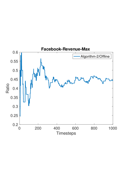
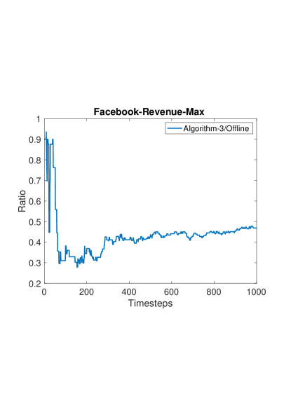
(a) (b)

Figure 1: Performance ratio for online revenue maximization over (a) a down-closed polytope; and (b) a general polytope.

In our setting, we consider the online variant of the revenue maximization on a social network where at time $t$ the weight of an edge is given $w^{t}_{ij}\in\{0,1\}$. The experiments are performed on the Facebook dataset that contains $20$K users (vertices) and $1$M relationships (edges). We choose the number of time steps to be $T=1000$. At each time $t\in{1,\ldots,T}$, we randomly uniformly select $2000$ vertices $V^{t}\subset V$, independently of $V^{1},\ldots,V^{t-1}$, and construct a batch $B_{t}$ with edge-weights $w^{t}_{ij}=1$ if and only if $i,j\in V^{t}$ and edge $(i,j)$ exists in the Facebook dataset. In case if $i$ or $j$ do not belong to $V^{t}$, $w^{t}_{ij}=0$. We set $p=0.0001$. In the first experiment, we impose a maximum investment constraint on the problem such that $\sum_{i\in V}x_{i}\leq 1$. This, in addition to $x_{i}\geq 0,\forall i\in V$ constitutes a down-closed feasible convex set. For the general convex set, we impose an additional minimum investment constraint on the problem such that $\sum_{i\in V}x_{i}\geq 0.1$.

For comparison purposes, we chose (offline) Frank-Wolfe algorithm as the benchmark. This algorithm is shown to be competitive both in theory and in practice for maximizing (offline) non-monotone DR-submodular functions over down-closed convex sets [1] and over general convex sets [14]. In Figure 1 we show the ratio of between the objective value achieved by the online algorithm and that of the benchmark over the down-closed convex set (Figure 1(a)) and the general convex set (Figure 1(b)). These experiments conform with the theoretical guarantees.

7 Conclusion

In this paper, we considered the regret minimization problems while maximization online arriving non-monotone DR-submodular functions over convex sets. We presented online algorithms that achieve a $1/e$-approximation and $1/2$-approximation ratios with the regret of $O(T^{2/3})$ and $O(\sqrt{T})$ for maximizing DR-submodular functions over any down-closed convex set and over the hypercube, respectively. Both of these algorithms are built upon on our novel idea of lifting and solving the optimization problem (the inherent oracles) in higher dimension. Moreover, we presented an online algorithm that achieves an approximation guarantee (depending on the search space) for the problem of maximizing non-monotone continuous DR-submodular functions over a general convex set (not necessarily down-closed). Finally, we run experiments to verify the performance of our algorithms on a social revenue maximization problem on a Facebook user-relationship dataset. Interesting direction for future work is to consider the non-monotone DR-submodular maximization in the bandit setting by combining our approach with algorithms for monotone DR-submodular functions in [36].

Appendix A Removing Knowledge of $T$

In this section, we show how to remove the assumption on the knowledge of $T$ for Algorithm 3. The procedure for Algorithms 2 is similar. In particular, we use the standard doubling trick (for example [11]) where Algorithm 3 is invoked repeatedly with a doubling time horizon.

Input: A convex set $\mathcal{K}$ and Algorithm 3

1:  for $m=0,1,2,\ldots$ do

2:     $L\mathrel{\mathop{\mathchar 58\relax}}=2^{m+1}$

3:     Run Algorithm 3 with horizon $2^{m}$, from the $(2^{m}+1)$-th iteration to the $2^{m+1}$-th iteration.

4:     Let $\bm{x}^{t}$ for $2^{m}+1\leq t\leq 2^{m+1}$ be the solution fo Algorithm 3.

5:  end for

Algorithm 4 Meta-Frank-Wolfe with Doubling Trick

Theorem 4.

Given Theorem 3, the following inequality holds true for Algorithm 4:

$$\sum\limits_{t=1}^{T}\mathbb{E}\left[F^{t}(\bm{x}^{t})\right]\geq \left(\frac{1}{3\sqrt{3}}\right)(1-\|\bm{x}_{0}\|_{\infty})\max_{\bm{x}^{*}\in{\cal K}}\sum\limits_{t=1}^{T}F^{t}(\bm{x}^{*})-O\biggl{(}\frac{(\beta D+G+\sigma)DT}{\ln T}\biggr{)}$$

Proof.

From Theorem 3, for each $m$, it follows that

$$\sum\limits_{t=2^{m}+1}^{2^{m+1}}\mathbb{E}\left[F^{t}(\bm{x}^{t})\right]\geq \left(\frac{1}{3\sqrt{3}}\right)(1-\|\bm{x}_{0}\|_{\infty})\max_{\bm{x}^{*}\in{\cal K}}\sum\limits_{t=2^{m}+1}^{2^{m+1}}F^{t}(\bm{x}^{*})-O\biggl{(}\frac{(\beta D+G+\sigma)D2^{m+1}}{(m+1)\ln 2}\biggr{)}.$$

Summing this quantity of $m=0,1,2,\ldots,\lceil\log_{2}(T+1)\rceil-1$, we have that

$$\sum\limits_{t=1}^{T} \mathbb{E}\left[F^{t}(\bm{x}^{t})\right]$$

$$\geq\left(\frac{1}{3\sqrt{3}}\right)(1-\|\bm{x}_{0}\|_{\infty})\max_{\bm{x}^{*}\in{\cal K}}\sum\limits_{t=1}^{T}F^{t}(\bm{x}^{*})-\sum_{m=0}^{\lceil\log_{2}(T+1)\rceil-1}O\biggl{(}\frac{(\beta D+G+\sigma)D2^{m+1}}{(m+1)\ln 2}\biggr{)}$$

$$\geq\left(\frac{1}{3\sqrt{3}}\right)(1-\|\bm{x}_{0}\|_{\infty})\max_{\bm{x}^{*}\in{\cal K}}\sum\limits_{t=1}^{T}F^{t}(\bm{x}^{*})-\sum_{m=0}^{\lceil\log_{2}(T+1)\rceil-1}O\biggl{(}\frac{(\beta D+G+\sigma)D2^{m+1}}{\ln 2}\biggr{)}$$

$$\geq\left(\frac{1}{3\sqrt{3}}\right)(1-\|\bm{x}_{0}\|_{\infty})\max_{\bm{x}^{*}\in{\cal K}}\sum\limits_{t=1}^{T}F^{t}(\bm{x}^{*})-O\biggl{(}\frac{(\beta D+G+\sigma)D}{\ln 2}\biggr{)}\sum_{m=1}^{\lceil\log_{2}(T+1)\rceil}\left(\frac{2^{m}}{m}\right)$$

$$\geq\left(\frac{1}{3\sqrt{3}}\right)(1-\|\bm{x}_{0}\|_{\infty})\max_{\bm{x}^{*}\in{\cal K}}\sum\limits_{t=1}^{T}F^{t}(\bm{x}^{*})-O\biggl{(}\frac{(\beta D+G+\sigma)D}{\ln 2}\biggr{)}\frac{2.2^{\lceil\log_{2}(T+1)\rceil}}{\lceil\log_{2}(T+1)\rceil}$$

$$\geq\left(\frac{1}{3\sqrt{3}}\right)(1-\|\bm{x}_{0}\|_{\infty})\max_{\bm{x}^{*}\in{\cal K}}\sum\limits_{t=1}^{T}F^{t}(\bm{x}^{*})-O\biggl{(}\frac{(\beta D+G+\sigma)DT}{\ln T}\biggr{)}.$$

∎

References

• [1] Andrew An Bian, Kfir Levy, Andreas Krause, and Joachim M. Buhmann. Non-monotone continuous DR-submodular maximization: Structure and algorithms. In Neural Information Processing Systems (NIPS), 2017.
• [2] Andrew An Bian, Baharan Mirzasoleiman, Joachim Buhmann, and Andreas Krause. Guaranteed non-convex optimization: Submodular maximization over continuous domains. In Artificial Intelligence and Statistics, pages 111–120, 2017.
• [3] Yatao Bian, Joachim Buhmann, and Andreas Krause. Optimal continuous DR-submodular maximization and applications to provable mean field inference. In Proceedings of the 36th International Conference on Machine Learning, pages 644–653, 2019.
• [4] Stephen Boyd and Lieven Vandenberghe. Convex optimization. Cambridge university press, 2004.
• [5] Niv Buchbinder and Moran Feldman. Deterministic algorithms for submodular maximization problems. ACM Transactions on Algorithms (TALG), 14(3):32, 2018.
• [6] Niv Buchbinder, Moran Feldman, Joseph Seffi, and Roy Schwartz. A tight linear time (1/2)-approximation for unconstrained submodular maximization. SIAM Journal on Computing, 44(5):1384–1402, 2015.
• [7] Gruia Calinescu, Chandra Chekuri, Martin Pál, and Jan Vondrák. Maximizing a monotone submodular function subject to a matroid constraint. SIAM Journal on Computing, 40(6):1740–1766, 2011.
• [8] Chandra Chekuri, TS Jayram, and Jan Vondrák. On multiplicative weight updates for concave and submodular function maximization. In Proc. Conference on Innovations in Theoretical Computer Science, pages 201–210, 2015.
• [9] Lin Chen, Christopher Harshaw, Hamed Hassani, and Amin Karbasi. Projection-free online optimization with stochastic gradient: From convexity to submodularity. In Proceedings of the 35th International Conference on Machine Learning, pages 814–823, 2018.
• [10] Lin Chen, Hamed Hassani, and Amin Karbasi. Online continuous submodular maximization. In Proc. 21st International Conference on Artificial Intelligence and Statistics (AISTAT), 2018.
• [11] Lin Chen, Mingrui Zhang, and Amin Karbasi. Projection-free bandit convex optimization. In Proc. 22nd Conference on Artificial Intelligence and Statistics, pages 2047–2056, 2019.
• [12] Josip Djolonga and Andreas Krause. From map to marginals: Variational inference in bayesian submodular models. In Advances in Neural Information Processing Systems, pages 244–252, 2014.
• [13] Josip Djolonga, Sebastian Tschiatschek, and Andreas Krause. Variational inference in mixed probabilistic submodular models. In Advances in Neural Information Processing Systems, pages 1759–1767, 2016.
• [14] Christoph Dürr, Nguyen Kim Thang, Abhinav Srivastav, and Léo Tible. Non-monotone dr-submodular maximization: Approximation and regret guarantees. In Proc. 29th International Joint Conference on Artificial Intelligence (IJCAI), 2020.
• [15] Ethan Elenberg, Alexandros G Dimakis, Moran Feldman, and Amin Karbasi. Streaming weak submodularity: Interpreting neural networks on the fly. In Advances in Neural Information Processing Systems, pages 4044–4054, 2017.
• [16] Ethan R Elenberg, Rajiv Khanna, Alexandros G Dimakis, Sahand Negahban, et al. Restricted strong convexity implies weak submodularity. The Annals of Statistics, 46(6B):3539–3568, 2018.
• [17] Moran Feldman, Joseph Naor, and Roy Schwartz. A unified continuous greedy algorithm for submodular maximization. In Proc. 52nd Symposium on Foundations of Computer Science (FOCS), pages 570–579, 2011.
• [18] Daniel Golovin and Andreas Krause. Adaptive submodularity: Theory and applications in active learning and stochastic optimization. Journal of Artificial Intelligence Research, 42:427–486, 2011.
• [19] Manuel Gomez Rodriguez, Jure Leskovec, and Andreas Krause. Inferring networks of diffusion and influence. In Proc. 16th ACM SIGKDD international conference on Knowledge discovery and data mining, pages 1019–1028, 2010.
• [20] Andrew Guillory and Jeff A Bilmes. Simultaneous learning and covering with adversarial noise. In ICML, volume 11, pages 369–376, 2011.
• [21] Hamed Hassani, Mahdi Soltanolkotabi, and Amin Karbasi. Gradient methods for submodular maximization. In Advances in Neural Information Processing Systems, pages 5841–5851, 2017.
• [22] Elad Hazan. Introduction to online convex optimization. Foundations and Trends® in Optimization, 2(3-4):157–325, 2016.
• [23] Shinji Ito and Ryohei Fujimaki. Large-scale price optimization via network flow. In Advances in Neural Information Processing Systems, pages 3855–3863, 2016.
• [24] David Kempe, Jon Kleinberg, and Éva Tardos. Maximizing the spread of influence through a social network. In Proc. 9th ACM SIGKDD international conference on Knowledge discovery and data mining, pages 137–146, 2003.
• [25] Alex Kulesza, Ben Taskar, et al. Determinantal point processes for machine learning. Foundations and Trends® in Machine Learning, 5(2–3):123–286, 2012.
• [26] Hui Lin and Jeff Bilmes. A class of submodular functions for document summarization. In Proc. 49th Meeting of the Association for Computational Linguistics: Human Language Technologies-Volume 1, pages 510–520, 2011.
• [27] Vahab Mirrokni, Renato Paes Leme, Adrian Vladu, and Sam Chiu-wai Wong. Tight bounds for approximate carathéodory and beyond. In Proc. 34th International Conference on Machine Learning, pages 2440–2448, 2017.
• [28] Aryan Mokhtari, Hamed Hassani, and Amin Karbasi. Conditional gradient method for stochastic submodular maximization: Closing the gap. In Procs of the International Conference on Artificial Intelligence and Statistics, volume 84, pages 1886–1895, 2018.
• [29] Rad Niazadeh, Tim Roughgarden, and Joshua R Wang. Optimal algorithms for continuous non-monotone submodular and dr-submodular maximization. In Neural Information Processing Systems (NIPS), 2018.
• [30] Tim Roughgarden and Joshua R Wang. An optimal learning algorithm for online unconstrained submodular maximization. In Conference On Learning Theory, pages 1307–1325, 2018.
• [31] Adish Singla, Ilija Bogunovic, Gábor Bartók, Amin Karbasi, and Andreas Krause. Near-optimally teaching the crowd to classify. In ICML, pages 154–162, 2014.
• [32] Tasuku Soma and Yuichi Yoshida. Non-monotone dr-submodular function maximization. In Proceedings of the Thirty-First AAAI Conference on Artificial Intelligence, 2017.
• [33] Matthew Staib and Stefanie Jegelka. Robust budget allocation via continuous submodular functions. In International Conference on Machine Learning, pages 3230–3240, 2017.
• [34] Matthew Streeter and Daniel Golovin. An online algorithm for maximizing submodular functions. In Advances in Neural Information Processing Systems, pages 1577–1584, 2009.
• [35] Jan Vondrák. Symmetry and approximability of submodular maximization problems. SIAM Journal on Computing, 42(1):265–304, 2013.
• [36] Mingrui Zhang, Lin Chen, Hamed Hassani, and Amin Karbasi. Online continuous submodular maximization: From full-information to bandit feedback. In Advances in Neural Information Processing Systems, pages 9206–9217, 2019.