A coherent router for quantum networks

Abstract

Scalable quantum information processing will require quantum networks of qubits with the ability to coherently transfer quantum states between the desired sender and receiver nodes. Here we propose a scheme to implement a quantum router that can direct quantum states from an input qubit to a preselected output qubit. The path taken by the transferred quantum state is controlled by the state of one or more ancilla qubits. This enables both directed transport between a sender and a number of receiver nodes, and generation of distributed entanglement in the network. We demonstrate the general idea using a two-output setup and discuss how the quantum routing may be expanded to several outputs. We also present a possible realization of our ideas with superconducting circuits.

Introduction

The transfer of quantum information between different quantum processing units will be an integral part of possible future quantum technology. While photons will play the decisive role for long-range transfer Cirac et al. (1997); Ursin et al. (2007); Kimble (2008), the short-range transport of quantum states is more likely to be accomplished via stationary information channels such as chains and networks of coupled qubits Kielpinski et al. (2002); Bose (2007); Kay (2010). Since the seminal work of Bose Bose (2003), many studies have explored how to accomplish high-fidelity transfer of quantum states through a spin or qubit network Nikolopoulos et al. (2004); Subrahmanyam (2004); Christandl et al. (2004); Albanese et al. (2004); Wójcik et al. (2005); Campos Venuti et al. (2007); Di Franco et al. (2008a, b); Wu et al. (2009); Yao et al. (2011); Kay (2011); Apollaro et al. (2012); Petrosyan et al. (2010); Georgios M. Nikolopoulos .

State transfer protocols in such networks typically rely on tuning nearest-neighbor couplings and local fields, either statically or dynamically, in order to maximize the fidelity of moving a quantum state across the network in minimum time. Controlling the individual qubit energies is usually done with the external classical fields, while couplings between the qubits are tuned via judicious engineering of the inter-qubit interactions Benjamin and Bose (2003); Banchi et al. (2011).

Since a larger quantum processing unit is likely to consists of several smaller devices or subprocessors, it is crucial to have a quantum routing system for selective high-fidelity state transfer and entanglement sharing between a sender and a distinct receiver in a network. This issue has previously been considered in several different contexts, including coupled harmonic systems Plenio et al. (2004), external flux threading Bose et al. (2005), local field adjustments in spin systems Wójcik et al. (2007); Facer et al. (2008); Nikolopoulos (2008); Chudzicki and Strauch (2010); Pemberton-Ross et al. (2010); Yung (2011), using local periodic field modulation Zueco et al. (2009) to manipulate tunneling rates Grossmann et al. (1991); Grifoni and Hänggi (1998); Della Valle et al. (2007); Creffield (2007), and using optimal control techniques at local sites Pemberton-Ross et al. (2010). The common theme of all of these previous proposals is that they require a considerable amount of careful external control in order to perform the routing of quantum states and entanglement.

In the present work we propose to tune the coupling between the input and the desired output qubits using ancilla qubits. The internal state of the ancilla qubit controls the the direction of the quantum state transfer, serving thus as a quantum router.

The great advantage of our scheme is that the ancilla qubits may be in superposition or entangled states, allowing the router to sent the quantum states into a superposition of different directions. Hence, the process of routing is done in a completely quantum mechanical manner. In combination with, e.g., a set of controllable swapping gates Marchukov et al. (2016); Rasmussen et al. (2019), quantum routers may be a starting point for constructing physical quantum processing devices analogously to classical circuit designs.

We first discuss the simplest realization of the router, with just two output qubits. We then describe a router for more than two output qubits. Finally, we propose a concrete realization of a quantum router using superconducting circuits You and Nori (2005); Devoret and Schoelkopf (2013). The qubit model used here is general and our routing scheme can also be implemented in numerous other platforms.

Router with two outputs

To illustrate the dynamics of the router, we start by considering the router with two output qubits. The most elementary quantum router consists of four qubits: The input qubit, the two output qubits and an ancilla qubit that controls the direction of the state transfer from the input to the desired output. We initialize the two output qubits in their ground state $\ket{0}$, while the input and control qubits are initialized in states $\ket{\psi_{I}}$ and $\ket{\psi_{C}}$ respectively. We write the initial state of the combined system as $\ket{i}=\ket{\psi_{I}{}}\ket{00}\ket{\psi_{C}}$. The router is then constructed in such a way that if the control qubit is in state $\ket{\psi_{C}}=\ket{0}$ the input state is moved to the first output qubit, and if the control is in state $\ket{\psi_{C}}=\ket{1}$ the input state is moved to the second output qubit.

$$\begin{split}\ket{\psi_{I}{}}\ket{00}\ket{0}&\rightarrow\ket{0}\ket{\psi_{I}{}0}\ket{0},\\ \ket{\psi_{I}{}}\ket{00}\ket{1}&\rightarrow\ket{0}\ket{0\psi_{I}{}}\ket{1}.\end{split}$$ (1)

In general, if the control qubit is in a superposition state $\ket{\psi_{C}}=\alpha\ket{0}+\beta\ket{1}$, where $\left|\alpha\right|^{2}+\left|\beta\right|^{2}=1$, we have

$$\ket{\psi_{I}{}}\ket{00}\ket{\psi_{C}}\rightarrow\alpha\ket{0}\ket{\psi_{I}{}0}\ket{0}+\beta\ket{0}\ket{0\psi_{I}{}}\ket{1}.$$ (2)

This creates entanglement between the control qubit and the output qubits. Entanglement is a crucial resource in many quantum algorithms and we will show below how the router can be modified such that different types of entanglement are achieved.

Figure 1(a) illustrates the system. The Hamiltonian of the quantum router can be written as

$$\begin{split}\hat{H}{}=&-\frac{\Delta_{1}}{2}\sigma^{z}_{1}-\frac{\Delta_{2}}{2}\sigma^{z}_{2}+J^{z}\left(\sigma^{z}_{1}+\sigma^{z}_{2}\right)\sigma_{C}^{z}\\ &+\frac{J^{x}}{2}\left[\sigma^{x}_{I}\left(\sigma^{x}_{1}+\sigma^{x}_{2}\right)+\sigma^{y}_{I}\left(\sigma^{y}_{1}+\sigma^{y}_{2}\right)\right],\end{split}$$ (3)

where $\sigma^{x}=\ket{0}\bra{1}+\ket{1}\bra{0}$, $\sigma^{y}=-i\ket{0}\bra{1}+i\ket{1}\bra{0}$ and $\sigma^{z}=\ket{0}\bra{0}-\ket{1}\bra{1}$ are the Pauli spin operators in the computational basis $\{\ket{0},\ket{1}\}$ of the qubits. The subscript $I{}$ indicates the input qubit, while subscripts $1$ and $2$ indicate the output qubits, and $C$ the control qubit. The $\ket{0}$-$\ket{1}$ transition frequencies of the output qubits (relative to that of the input qubit) are $\Delta_{1,2}$, and the transverse and longitudinal coupling strengths are denoted as $J^{x}$ and $J^{z}$ respectively. The first interaction term with strength $J^{z}$ enables the control qubit to shift the frequencies of the two output qubits. The second interaction term has strength $J^{x}$ and transversely couples the input qubit to the output qubits. This allows the input qubit to swap an excitation with an output qubit, if their frequencies are resonant. We require the energy shift due to the interaction with the control qubit to be much larger than the transverse coupling $J^{z}\gg J^{x}$.

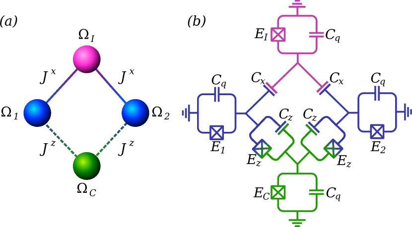
Figure 1: (a) Schematic illustration of the router system with two output qubits. The solid lines represent transverse $XX$-type couplings and the dashed lines represent longitudinal $ZZ$-type couplings. The purple sphere represents the input qubit, the blue spheres represent the output qubits, and the green sphere is the ancilla qubit. Depending on the state of the ancilla qubit, the state of the input qubit is sent to either first or second output qubit, or their superposition. (b) Possible circuit implementation. The superconducting circuit consists of four transmon qubits connected in a square. Two parallel lines indicates capacitors, while the crossed boxes indicate Josephson junctions. The different parts of the system are colored according to their role, as per (a).

We assume that the transition frequencies of the output qubits can be independently tuned. Depending on the state of the control qubit, the router should send the state of the input qubit to one of the output qubits. To realize this behavior, we set the detunings as

$$\Delta_{1}=-\Delta_{2}=2J^{z}.$$ (4)

The diagonal part of the Hamiltonian in Eq. 3 then becomes

$$\begin{split}\hat{H}_{\text{diag}}=\begin{cases}0\sigma^{z}_{1}+2J^{z}\sigma^{z}_{2}&\text{for }\langle\sigma^{z}_{C}\rangle=1\\ -2J^{z}\sigma^{z}_{1}+0\sigma^{z}_{2}&\text{for }\langle\sigma^{z}_{C}\rangle=-1.\end{cases}\end{split}$$ (5)

When the control qubit is in the state $\ket{0}$, corresponding to $\langle\sigma^{z}_{C}\rangle=1$, the input and the first output qubit are resonant while the second output qubit is detuned. If the detuning is significantly larger than the transverse coupling strength, i.e. $|4J^{z}/J^{x}|\gg 1$, transfer from the input qubit to second output qubit will be suppressed, while excitations can hop resonantly from the input to the first output qubit. If, on the other hand, the control qubit is in the orthogonal $\ket{1}$ state, the excitation can hop from the input to the second output qubit, while transfer to the first output qubit is suppressed.

More formally, we may write the Hamiltonian in a frame rotating with its diagonal part as

$$\frac{\hat{H}_{\text{rot}}}{J^{x}} =\sigma^{-}_{I}\sigma^{+}_{1}e^{2iJ^{z}\left(\sigma^{z}_{C}-1\right)t}+\sigma^{-}_{I}\sigma^{+}_{2}e^{2iJ^{z}\left(\sigma^{z}_{C}+1\right)t}+\text{h.c.}$$

$$\approx\sigma^{-}_{I}\sigma^{+}_{1}\ket{0_{C}}\bra{0_{C}}+\sigma^{-}_{I}\sigma^{+}_{2}\ket{1_{C}}\bra{1_{C}}+\text{h.c.},$$ (6)

where we have used the rotating wave approximation in conjunction with the assumption $|4J^{z}/J^{x}|\gg 1$ in order to obtain the final expression. At time $T=\pi/(2J^{x})$ the transfer is complete and the transformation is described by the unitary operator

$$\hat{U}_{T}=\exp\Big{\{} -i\frac{\pi}{2}\big{(}\sigma^{-}_{I}\sigma^{+}_{1}\ket{0_{C}}\bra{0_{C}}$$ (7)

$$+\sigma^{-}_{I}\sigma^{+}_{2}\ket{1_{C}}\bra{1_{C}}+\text{h.c.}\big{)}\Big{\}}.$$

Note that this unitary transformation is indeed capable of creating entanglement when the control qubit is in a superposition state, as in Eq. 2.

To characterize the performance of the quantum router, we calculate the average process fidelity, defined as Nielsen and Chuang (2010); Nielsen (2002); Horodecki et al. (1999); Schumacher (1996)

$$\bar{F}=\int d\psi\bra{\psi}\hat{U}_{T}^{\dagger}\mathcal{E}(\psi)\hat{U}_{T}\ket{\psi},$$ (8)

where the integration is performed over the subspace of all possible initial states and $\mathcal{E}$ is the quantum map realized by our system. We initialize the two output qubits in state $\ket{0}$ so the subspace of initial states is spanned by $\left\{\ket{0}\ket{00}\ket{0},\allowbreak\ket{1}\ket{00}\ket{0},\allowbreak\ket{0}\ket{00}\ket{1},\allowbreak\ket{1}\ket{00}\ket{1}\right\}$. The average fidelity is then calculated with the QuTiP Python toolbox Johansson et al. (2012) using the procedure described in Pedersen et al. (2007). In all calculations, we have $J^{z}/(2\pi)=10\text{MHz}$ and the relaxation and decoherence times are $T_{1}=T_{2}=30\mu$s Wendin (2017). In Fig. 2 we show the average process fidelity at the transfer time $T=\pi/(2J^{x})$. When $|J^{x}|=|J^{z}|$ the most detrimental source of error is transfer to the wrong output qubit, since the detuning induced by the control qubit is not large enough to completely suppress the hopping interaction connecting the input and closed output qubits. In this regime, the error due to decoherence is comparatively small, which is due to the fact that the transfer times are shorter for larger $J^{x}$. For larger values of $|J^{z}/J^{x}|$, transfer to the closed output qubit is stronger suppressed, and the average process fidelity approaches unity, if we neglect decoherence. But since the transfer time also increases, decoherence becomes the dominant source of error. With our choice of parameters, the maximum fidelity is $\bar{F}_{max}=0.9907$ at $|J^{z}/J^{x}|=4.192$.

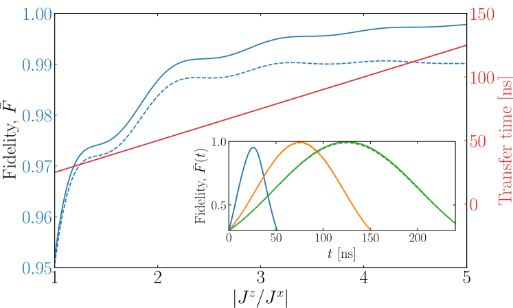
Figure 2: Average fidelity of the two-output router as a function of the coupling ratio. The blue solid line shows the average fidelity at time $t=\pi/(2J^{x})$. The dashed lines are the average fidelity with relaxation and coherence time of $T_{1}=T_{2}=30\mu$s. The red line is the corresponding transfer time. In all calculations we have used $J^{z}/(2\pi)=10$MHz. Insert: Time dependence of the state transfer of the two-output router for $J^{z}/J^{x}=1$ (blue), $J^{z}/J^{x}=3$ (yellow) and $J^{z}/J^{x}=5$ (green).

Concatenated routers

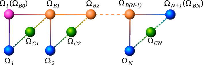
Figure 3: (a) Schematic illustration of a concatenated router with N+1 output ports. The purple sphere is the input qubit, the blue spheres are the output qubits, the green spheres are the control qubits, and the orange spheres are bus qubits, i.e., qubits which act both as input and output qubits.

The number of output ports of the router can be scaled in several ways (see Supplementary material sup ). Here we describe a scheme in which $N$ routers are concatenated as shown on Fig. 3 where one output of each router serves as the input qubit for the next one. We refer to these qubits as the bus qubits.

The concatenated router operates in (time) steps. Step 0: Initialize the input qubit in a given state $\ket{\psi}$. Step 1: The state will either move down to the first output or right to the first bus qubit, depending on the state of the first control qubit. After the state have been transferred, i.e., at $t=T$, the input qubit is closed by detuning it from the bus qubit. Step 2: The state moves either down to the second output qubit or continues right to the second bus qubit, depending on the state of the second control qubit. Step 3: Detune the second bus qubit from the first bus qubit at time $t=2T$. The procedure proceeds as above until the state moves down into one of the $N$ output qubits or it arrives at the last output qubit $N+1$.

This process can be expressed through a Hamiltonian with time-dependent detunings. The static part of the Hamiltonian is

$$\hat{H}{}= J^{z}\sum_{i=1}^{N}\left[\sigma_{i}^{z}(\sigma_{C_{i}}^{z}+1)+\sigma_{B_{i}}(\sigma_{C_{i}}^{z}-1)\right]$$ (9)

$$+\frac{J^{x}}{2}\sum_{i=1}^{N}\left[\sigma_{B_{i-1}}^{x}(\sigma_{i}^{x}+\sigma_{B_{i}}^{x})+\sigma_{B_{i-1}}^{y}(\sigma_{i}^{y}+\sigma_{B_{i}}^{y})\right],$$

where we denote the bus’ qubits $\sigma_{B}^{x,y,z}$, and the zero’th bus qubit is the input qubit, while the $N$’th bus qubit is the final output qubit. The time-dependent part of the Hamiltonian is

$$\hat{H}{}(t)= \Delta\sum_{i=1}^{N}\left[\sigma_{B_{i-1}}^{z}+\sigma_{B_{i}}^{z}+\sum_{j=1}^{i}\sigma_{j}^{z}\right]$$ (10)

$$\qquad\times\left[\theta(t-(i-1)T)-\theta(t+iT)\right],$$

where $\Delta$ is the detuning, and $\theta(t)$ is the Heaviside step function. For the process to function properly, we must ensure that $|\Delta|\gg|J^{x}|$ and $|2J^{z}\pm\Delta|\gg|J^{x}|$. Thus, an excitation starting in the input qubit will move down the chain of bus qubits in discrete time-steps until it encounters a control qubit in state $\ket{0}$ and moves to the associated output qubit, where it will remain for the rest of the process.

Implementation using superconducting circuits

Table 1: Physical parameters used for our example implementation of the quantum router.

$\frac{C_{q}}{\text{fF}}$	$\frac{C_{z}}{\text{fF}}$	$\frac{C_{x}}{\text{fF}}$	$\frac{E_{I}}{2\pi\text{GHz}}$	$\frac{E_{1}}{2\pi\text{GHz}}$	$\frac{E_{2}}{2\pi\text{GHz}}$	$\frac{E_{C}}{2\pi\text{GHz}}$	$\frac{E_{z}}{2\pi\text{GHz}}$
80.0	13.7	0.082	19.52	19.22	19.52	38.74	3.46

Superconducting circuits present a promising platform to implement the quantum router. Specifically, we propose an implementation using transmon qubit architecture as shown in Fig. 1(b). The circuit consists of four transmon qubits, each of which can be made flux-tunable by substituting the Josephson Junction with a SQUID. The two output qubits (blue) are coupled to the control qubit (green) each through a Josephson junction and a capacitor in parallel. The nonlinearity of this Josephson Junction provides the main mechanism behind the $ZZ$-type coupling between outputs and control. A tunable version of this coupler has been investigated experimentally, and it has been shown that the transversal coupling could be made negligible compared to the longitudinal coupling Kounalakis et al. (2018). In our scheme, the transverse coupling between the output qubits and control is much smaller than their relative detuning such that there will be no exchange of excitations between them.

By using second order perturbation theory, we derive an effective Hamiltonian for the circuit (see supplementary material sup )

$$\begin{split}\hat{H}_{\textbf{eff}}^{\textbf{circ}}=&-\frac{\Delta_{1}}{2}\sigma^{z}_{1}-\frac{\Delta_{2}}{2}\sigma^{z}_{2}+J^{z}\left(\sigma^{z}_{1}+\sigma^{z}_{2}\right)\sigma_{C}^{z}\\ &+\frac{J^{x}}{2}\left[\sigma^{x}_{I}\left(\sigma^{x}_{1}+\sigma^{x}_{2}\right)+\sigma^{y}_{I}\left(\sigma^{y}_{1}+\sigma^{y}_{2}\right)\right]\\ &+\left(\frac{J^{x}_{12}}{2}+\frac{J^{xz}_{12}}{2}\sigma^{z}_{C}\right)\left(\sigma^{x}_{1}\sigma^{x}_{2}+\sigma^{y}_{1}\sigma^{y}_{2}\right),\end{split}$$ (11)

where the three last terms arise from the second order interactions between outputs and control. A numerical modeling of the full circuit Hamiltonian with the parameters shown in Table 1 gives us a longitudinal coupling of $J^{z}=-9.95\cdot(2\pi\text{MHz})$ and a transversal input/output coupling of $J^{x}=2.78(2\pi\text{MHz})$ with appropriate detunings of the outputs, as explained in the introduction. The three remaining couplings are all much smaller than $J^{x}$ and can thus be neglected for our purposes.

Conclusion

We have presented a simple implementation of a quantum router with quantum control, and analyzed it analytically and numerically. By utilizing a relatively strong interaction with a control qubit, state transfer to the undesired output qubit can be suppressed, and we achieve selective transfer fidelity above 0.99, even when including the effects of dephasing and relaxation. We have also presented a scalable scheme that can extend the router to an arbitrary number of outputs. Finally, we have presented a possible realization of the router using a superconducting circuit. Our simple routing scheme is capable of distributing entanglement between distant qubits which is highly useful for short-range (on-chip) quantum communications.