Sum Rule of Quantum Uncertainties: Coupled Harmonic Oscillator System with Time-Dependent Parameters
Abstract
Uncertainties and are analytically derived in an -coupled harmonic oscillator system when spring and coupling constants are arbitrarily time-dependent and each oscillator is in an arbitrary excited state. When , those uncertainties are shown as just arithmetic average of uncertainties of two single harmonic oscillators. We call this property as “sum rule of quantum uncertainty”. However, this arithmetic average property is not generally maintained when , but it is recovered in -coupled oscillator systems if and only if quantum numbers are equal. The generalization of our results to a more general quantum system is briefly discussed.
I Introduction
Uncertaintyuncertainty ; kennard1927 ; robertson1929 ; Busch2007 and entanglementschrodinger-35 ; text ; horodecki09 are two major cornerstones of quantum mechanics. These characteristics cause quantum mechanics to differ from classical mechanics. Quantum uncertainty provides a limit on the precision of measurement for incompatible observables. The most typical expression of uncertainty relation is , where is the standard deviation. Recently, researchers have analyzed different expressions of uncertainty relations, such as entropic uncertainty relationsWehner2010 ; Coles2017 from the context of quantum information and generalized uncertainty principleGUP from the context of Planck scale physics. Even though entanglement has been studied since the discovery of quantum mechanicsschrodinger-35 , it has been extensively explored for the last few decades with the development of quantum technology. Entanglement is used as a physical resource in various quantum information processing, such as quantum teleportationteleportation ; Luo2019 , superdense codingsuperdense , quantum cloningclon , quantum cryptographycryptography ; cryptography2 , quantum metrologymetro17 , and quantum computerqcreview ; computer . Furthermore, with many researchers trying to realize such quantum information processing in the laboratory for the last few decades, quantum cryptography and quantum computer seems to approaching the commercial levelwhite ; ibm .
Although these two phenomena seem to be distinct properties of quantum mechanics, there is some connection, albeit unclear, between them because of the fact that both are strongly dependent on the interaction between subsystems. For example, the uncertainty of a given system was computed in Ref.han97 ; han99 to discuss on the effect of the Feynman’s rest of universefeyman72 . The ignoring of the effect of the rest of the universe was shown to increase uncertainty and entropy in the target system (system in which we are interested). In other words, if the target system is one of subsystems of a whole system and it interacts with other subsystems, its uncertainty and entanglement monotonically increase with increasing interaction strength. More specifically, let us consider two coupled harmonic oscillator system, with the following Hamiltonian:
| (1) |
If we assume that the two oscillators, say and , were in each ground state, the uncertainty and entanglement of formation (EoF)benn96 are both given bypark18
| (2) |
where and . This shows that both and increase with increasing the coupling constant . Thus, in this case, uncertainty and entanglement are implicitly related to each other via . Duan et al.criterion used quantum uncertainty to provide a sufficient criterion for entanglement in continuous variable systems. Mandilara and Cerfcerf12 showed that the uncertainty relation for all eigenstates in the single harmonic oscillator system is saturated with respect to Gaussianity.
So far, EoF cannot be exactly computed in the coupled harmonic oscillator system except in the ground state because of the non-Gaussian nature of exciting states111The Rényi- entropies of few non-Gaussian states have been derived in Ilki-18 .. As EoF and uncertainty exhibit similar behavior, as shown in Eq. (2), the uncertainty may be used as a measure of entanglement after appropriate rescaling if EoF cannot be computed exactly. Therefore, in order to understand the entanglement more profoundly in the continuous variable system, it is important to examine the uncertainty of the arbitrary excited states in the coupled harmonic oscillator system.
In there any other similarity between EoF and uncertainty? EoF is believed to have the additivity propertyopen05 , even though the property has still not been solved completely. For mixed states, EoF is generally defined by a convex-roof methodbenn96 ; uhlmann99-1 as follows:
| (3) |
where the minimum is taken over all possible ensembles of pure states with . Let be two bipartite density matrices, and . If we regard as a bipartite state, where and belong to each party, Eq. (3) guarantees . The additivity conjecture of EoF is that the equality always holds; this has been demonstrated through various examples in additivity . In this paper, we show that uncertainty in the coupled harmonic oscillator system also has a particular additive property, which we call the sum rule. We present this sum rule in the coupled harmonic oscillator system when the parameters are arbitrarily time-dependent.
The paper is organized as follows. In Sec. II we derive and of arbitrary excited states by making use of explicit Wigner distribution in the single harmonic oscillator system when the frequency is arbitrary time-dependent. It is shown that the time-dependence of frequency as well as energy level increase the uncertainty . In Sec. III we examine the uncertainties in the two-coupled harmonic oscillator system when the parameters are arbitrarily time-dependent. In this section we derive the uncertainties and of the first or second oscillator when two oscillators are at the arbitrary excited states. It is shown that and are just the arithmetic average of uncertainties of two single oscillators. We call this additive property as ”sum rule of quantum uncertainties”. As a by-product, the purity function of the reduced state is explicitly computed in this section by making use of the reduced Wigner distribution function. In Sec. IV we examine the uncertainties in the -coupled harmonic oscillator system when the parameters are arbitrarily time-dependent. It is shown that the arithmetic average property of uncertainties arising at is not generally maintained when . However, this additive property is recovered when quantum numbers are equal. In Sec. V conclusion and further discussion are briefly given.
II Uncertainty for arbitrary excited state of single harmonic oscillator with arbitrary time-dependent frequency
We start with a simple single harmonic oscillator Hamiltonian with arbitrary time-dependent frequency: . This simple model is important for studying the squeezed states, which appear in various branches of physics, such as quantum opticswalls-83 ; loudon-87 ; wu-87 ; schnabel-17 and cosmologygrishchuk-90 ; grishchuk-93 ; einhorn-03 ; kiefer-07 . The time-dependent Schrödinger equation (TDSE) of this system was examined in detail in lewis68 ; rhode89 ; lohe09 ; pires-19 . The linearly independent solutions are expressed in the following formlewis68 ; lohe09 :
| (4) |
where and
| (5) |
In Eq. (4) is the -order Hermite polynomial and satisfies the nonlinear Ermakov equation,
| (6) |
with and . As shown in Eq. (4), plays the role of scaling the frequency. Solutions of the Ermakov equation were discussed in lohe09 ; pinney50 ; gritsev-10 ; campo-16 . If is time independent, is simply one. If is instantly changed as follows:
| (9) |
then becomes
| (10) |
Of course, for a more general case of , the nonlinear Ermakov equation should be solved numerically or approximately.
The -dimensional Wigner distribution functionfeyman72 ; noz91 is defined in terms of the phase space variables in the following form:
| (11) |
where , , and is a wave function of a given system. The Wigner distribution function is used to compute the expectation values. For example, the expectation value of can be computed by
| (12) |
Moreover, the Wigner distribution function has information on the substate of density matrix . If , the purity function of can be computed as
| (13) |
where .
To explicitly compute the Wigner distribution function of , we set and of Eq. (4) in Eq. (11). The integral in Eq. (11) can be computed by usingintegral
| (14) | |||
| (19) | |||
Then, the Wigner distribution function for can be written as follows:
| (20) | |||
| (23) | |||
where is a confluent hypergeometric function. It is straightforward to show that , which guarantees is the normalized pure state. By using the Wigner distribution function, it is straightforward to show that for non-negative integer , and
| (24) | |||
where and are gamma and hypergeometric functions. Thus, the uncertainties for and are
| (25) |
which yield an uncertainty relation
| (26) |
Thus, the time-dependence of as well as energy level increase the uncertainty .
III Uncertainty for arbitrary excited state of two-coupled harmonic oscillator system with arbitrary time-dependent parameters
Now, let us consider the Hamiltonian (1) again when and are arbitrarily time dependent. It is not difficult to show that the Hamiltonian is diagonalized by introducing normal coordinates and , and their conjugate momenta and with normal mode frequencies and , respectively. If two oscillators are in the and states, we will show in the following that the uncertainties for and () are just the arithmetic mean of two single oscillators; that is,
| (27) | |||
where (), and satisfy their own nonlinear Ermakov equations, with and . We will call this arithmetic average additivity as “sum rule of quantum uncertainty”.
To prove Eq. (27), we start with solutions of TDSE for in terms of , which is
| (28) | |||
where , , and . Now, let us compute the Wigner distribution functions of the system by setting in Eq. (11). If we change Eq. (28) into the original phase space variables and , and insert them into Eq. (11), the computation of the Wigner distribution function is highly complicated. However, this difficulty can be avoided. Since are orthogonal normal modes, they preserve the inner product and -dimensional volume elements. Thus, the Wigner distribution function for is simply reduced to
| (29) |
where is a Wigner distribution function of a single harmonic oscillator given in Eq. (20).
At this stage we want to digress little bit. Sometimes, we need to derive the lower-dimensional reduced Wigner distribution function to explore the properties of the reduced quantum state. Although we can compute the -dimensional Wigner distribution function quickly by using the normal mode, the derivation of the reduced -dimensional Wigner distribution function is very complicated problem. For example, let us consider ; here, the difficulty arises because is not invariant measure in the normal modes. Thus, we should compute the reduced Wigner distribution function by using the original coordinates and conjugate momenta. After long and tedious calculation, it is possible to show that
| (34) | |||
where
| (35) | |||
Thus, the reduced Wigner distribution function for is easily computed by
| (36) |
The purity function of the -oscillator is defined as , where is an effective state of the -oscillator derived by taking a partial trace to over -oscillator. Then, can be computed from as follows:
| (37) |
where . From Eq. (34) one can show directly by making use of simple binomial formula. Furthermore, it is possible to show that
| (42) | |||
| (47) | |||
where
| (48) | |||
If we define the ratios
| (49) |
they are summarized at Table I. We expect that and decrease with increasing because more excited states seem to be more mixed.
| too long |
Table I: The ratios and for
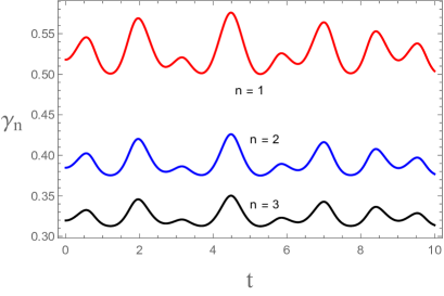
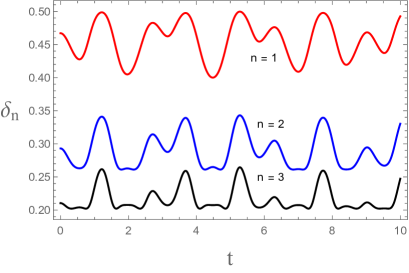
The time dependence of and is plotted in Fig. 1(a) and Fig. 1(b) when and . As expected, the figures exhibit that the effective states for the -oscillator is more and more mixed with increasing . Remarkably, this figure shows that the reduced state of is more mixed than that of .
IV Uncertainty for arbitrary excited state of -coupled harmonic oscillator system with arbitrary time-dependent parameters
To check whether the property of arithmetic average for uncertainties is maintained in a multi-coupled harmonic oscillator system or not, we first consider a three-coupled harmonic oscillator system with the following Hamiltonian:
| (50) |
The normal mode coordinates of is , , and with normal mode frequencies and . If three oscillators are in the , , and states, the -dimensional Wigner distribution function can be computed as follows:
| (51) |
where represent the conjugate momenta of and is the Wigner distribution function of the single harmonic oscillator given in Eq. (20). Of course, and are solutions for Ermakov equations for and , and and . Thus, Eq. (25) and Wigner distribution function (51) imply
| (52) | |||
Then, it is straightforward to show
| (53) | |||
Thus, the property of the arithmetic average in uncertainties is not maintained when . However, this property is recovered when .
Finally, let us consider the -coupled harmonic oscillator system with the following Hamiltonian:
| (54) |
This system is diagonalized by introducing the normal mode coordinates and with normal mode frequencies and . If oscillators are in the states, the -dimensional Wigner distribution function can be written as follows:
| (55) |
where represent the conjugate momenta of and is the Wigner distribution function of the single harmonic oscillator given in Eq. (20). Then, it is straightforward to show that
| (56) | |||
Eq. (56) can be shown to reproduces Eq. (27) and Eq. (53) when and if the quantum numbers , , and are replaced by , , and , respectively. If , one can show that and are independent of and they are just arithmetic average of uncertainties for each oscillator.
V Conclusions
In this paper we computed the uncertainties of and analytically in an -coupled harmonic oscillator system. When , these uncertainties are just the arithmetic average of uncertainties of two single harmonic oscillators. We call this property as “sum rule of quantum uncertainty”. However, this additive property is not generally maintained when but is recovered in an -coupled oscillator system only when quantum numbers are equal.
Our calculation can be generalized to a more general case. For example, let us consider the following Hamiltonian
| (57) | |||
In this case, the normal mode coordinates become
| (58) | |||
with and
| (59) |
Moreover, the normal mode frequencies are given by and . If the three oscillators are in the , , and exciting states, our procedure yields
| (60) | |||
where , , and . Of course are the scaling factors of . Similarly, the uncertainties can be computed explicitly by following the same procedure.
We do not know whether or not the sum rule of quantum uncertainty arising at is realized in other continuous variable systems such as -potential system. Also, we do not clearly understand whether or not the sum rule of uncertainty may have some implication on the additivity of entanglement. We hope to explore these issues in the future.
Quantum information processing with continuous variables has attracted considerable attention from both theoretical and experimental aspectsbraunstein-2005 ; adesso-2014 . Quantum uncertainties are closely connected to the inseparability criterion of a continuous-variable quantum systemcriterion ; simon-2000 . Furthermore, the distillation protocols to a maximally entangled state have already been suggested in Duan et al.duan-99-p and Giedke et al.giedke-2000 . We hope that our results on the explicit expressions of uncertainties may give valuable insight into the problem of continuous-variable quantum information processing.
References
- (1) W. Heisenberg, Über den anschaulichen Inhalt der quantentheoretischen Kinematik und Mechanik, Z. Phys. 43 (1927) 172.
- (2) E. H. Kennard, Zur Quantenmechanik einfacher Bewegungstypen, Z. Phys. 44 (1927) 326.
- (3) H. P. Robertson, The Uncertainty Principle, Phys. Rev. 34 (1929) 163.
- (4) P. Busch, T. Heinonen, and P. Lahti, Heisenberg’s uncertainty principle, Phys. Rep. 452, 155 (2007).
- (5) E. Schrödinger, Die gegenwärtige Situation in der Quantenmechanik, Naturwissenschaften, 23 (1935) 807.
- (6) M. A. Nielsen and I. L. Chuang, Quantum Computation and Quantum Information (Cambridge University Press, Cambridge, England, 2000).
- (7) R. Horodecki, P. Horodecki, M. Horodecki, and K. Horodecki, Quantum Entanglement, Rev. Mod. Phys. 81 (2009) 865 [quant-ph/0702225] and references therein.
- (8) S. Wehner and A. Winter, Entropic uncertainty relations–a survey, New J. Phys. 12, 025009 (2010).
- (9) P. J. Coles, M. Berta, M. Tomamichel, and S. Wehner, Entropic uncertainty relations and their applications, Rev. Mod. Phys. 89, 015002 (2017).
- (10) A. N. Tawfik and A. M. Diab, Review on Generalized Uncertainty Principle, Rept. Prog. Phys.78 (2015) 126001 [arXiv:1509.02436 (physics.gen-ph)] and references therein.
- (11) C. H. Bennett, G. Brassard, C. Crepeau, R. Jozsa, A. Peres and W. K. Wootters, Teleporting an Unknown Quantum State via Dual Classical and Einstein-Podolsky-Rosen Channles, Phys.Rev. Lett. 70 (1993) 1895.
- (12) Y. H. Luo et al., Quantum Teleportation in High Dimensions, Phys. Rev. Lett. 123 (2019) 070505 [arXiv:1906.09697 (quant-ph)].
- (13) C. H. Bennett and S. J. Wiesner, Communication via one- and two-particle operators on Einstein-Podolsky-Rosen states, Phys. Rev. Lett. 69 (1992) 2881.
- (14) V. Scarani, S. Lblisdir, N. Gisin and A. Acin, Quantum cloning, Rev. Mod. Phys. 77 (2005) 1225 [quant-ph/0511088] and references therein.
- (15) A. K. Ekert , Quantum Cryptography Based on Bell’s Theorem, Phys. Rev. Lett. 67 (1991) 661.
- (16) C. Kollmitzer and M. Pivk, Applied Quantum Cryptography (Springer, Heidelberg, Germany, 2010).
- (17) K. Wang, X. Wang, X. Zhan, Z. Bian, J. Li, B. C. Sanders, and P. Xue, Entanglement-enhanced quantum metrology in a noisy environment, Phys. Rev. A97 (2018) 042112 [arXiv:1707.08790 (quant-ph)].
- (18) T. D. Ladd, F. Jelezko, R. Laflamme, Y. Nakamura, C. Monroe, and J. L. O’Brien, Quantum Computers, Nature, 464 (2010) 45 [arXiv:1009.2267 (quant-ph)].
- (19) G. Vidal, Efficient classical simulation of slightly entangled quantum computations, Phys. Rev. Lett. 91 (2003) 147902 [quant-ph/0301063].
- (20) S. Ghernaouti-Helie, I. Tashi, T. Laenger, and C. Monyk, SECOQC Business White Paper, arXiv:0904.4073 (quant-ph).
- (21) see https://www.technologyreview.com/s/609451/ibm-raises-the-bar-with-a-50-qubit-quantum-computer/.
- (22) D. Han, Y. S. Kim, and M. E. Noz, Coupled Harmonic Oscillators and Feynman’s Rest of the Universe, cond-mat/9705029.
- (23) D. Han, Y. S. Kim, and M. E. Noz, Illustrative Example of Feynman’s Rest of the Universe, Am. J. Phys. 67 (1999) 61.
- (24) R. P. Feymann, Statistical Mechanics (Benjamin/Cummings, Reading, MA, 1972).
- (25) C. H. Bennett, D. P. DiVincenzo, J. A. Smokin and W. K. Wootters, Mixed-state entanglement and quantum error correction, Phys. Rev. A 54 (1996) 3824 [quant-ph/9604024].
- (26) DaeKil Park, Dynamics of entanglement and uncertainty relation in coupled harmonic oscillator system: exact results, Quant. Inf. Proc. 17 (2018) 147 [arXiv:1801.07070 (quant-ph)].
- (27) L. M. Duan, G. Giedke, J. I. Cirac, and P. Zoller, Inseparability criterion for continuous variable systems, Phys. Rev. Lett. 84 (2000) 2722 [quant-ph/9908056].
- (28) A. Mandilara and N. J. Cerf, Quantum uncertainty relation saturated by the eigenstates of the harmonic oscillator, Phys. Rev. A 86 (2012) 030102(R) [arXiv:1201.0453 (quant-ph)].
- (29) Ilki Kim, Rényi- entropies of quantum states in closed form: Gaussian states and a class of non-Gaussian states, Phys. Rev. E 97 (2018) 062141 [arXiv:1804.05980 (cond-mat)].
- (30) O. Krueger and R. F. Werner, Some Open Problems in Quantum Information Theory, quant-ph/0504166.
- (31) A. Uhlmann, Fidelity and concurrence of conjugate states, Phys. Rev. A 62 (2000) 032307 [quant-ph/9909060].
- (32) G. Vidal, W. Dür, and J. I. Cirac, Entanglement cost of mixed states, Phys. Rev. Lett. 89, (2002) 027091[quant-ph/0112131].
- (33) D. F. Walls, Squeezed states of light, Nature, 306 (5939) (1983) 141.
- (34) R. Loudon and P. L. Knigh, Squeezed Light, J. Mod. Optics, 34 (1987) 709.
- (35) L. A. Wu, M. Xiao, and H. J. Kimble, Squeezed states of light from an optical parametric oscillator, J. Opt. Soc. Am. B 4 (1987) 1465.
- (36) R, Schnabel, Squeezed states of light and their applications in laser interferometers, Phys. Rep. 684 (2017) 1 [arXiv:1611.03986 (quant-ph)].
- (37) L. P. Grishchuk and Y. V. Sidorov, Squeezed quantum states of relic gravitons and primordial density fluctuations, Phys. Rev. D 42 (1990) 3413.
- (38) L. P. Grishchuk, Quantum effects in cosmology, Classical and Quantum Gravity, 10 (1993) 2449 (gr-qc/9302036).
- (39) M. B. Einhorn and F. Larsen, Squeezed states in the de Sitter vacuum, Phys. Rev. D 68 (2003) 064002 (hep-th/0305056).
- (40) C. Kiefer, I. Lohmar, D. Polarski, and A. A. Starobinsky, Pointer states for primordial fluctuations in inflationary cosmology, Classical and Quantum Gravity, 24 (2007) 1699 (astro-ph/0610700).
- (41) H. R. Lewis Jr., and W. B. Riesenfeld, An Exact Quantum Theory of the Time‐Dependent Harmonic Oscillator and of a Charged Particle in a Time‐Dependent Electromagnetic Field, J. Math. Phys. 10 (1969) 1458.
- (42) X. Ma and W. Rhodes, Squeezing in harmonic oscillators with time-dependent frequencies, Phys. Rev. A 39 (1989) 1941.
- (43) M. A. Lohe, Exact time dependence of solutions to the time-dependent Schrödinger equation, J. Phys. A: Math. Theor. 42 (2009) 035307.
- (44) D. M. Tibaduiza, L. B. Pires, D. Szilard, A. L. C. Rego, C. A. D. Zarro and C. Farina, Exact algebraic solution for a quantum harmonic oscillator with time-dependent frequency, arXiv:1908.11006 [quant-ph].
- (45) E. Pinney, The nonlinear differential equation, Proc. Amer. Math. Soc. 1 (1950) 681.
- (46) V. Gritsev, P. Barmettler, and E. Demler Scaling approach to quantum non-equilibrium dynamics of many-body systems, New J. Phys. 12 (2010) 113005 [arXiv:0912.2744 (cond-mat)].
- (47) A. del Campo, Exact quantum decay of an interacting many-particle system: the Calogero–Sutherland model, New J. Phys. 18 (2016) 015014 [arXiv:1504.01620 (quant-ph)].
- (48) Y. S. Kim and M. E. Noz, Phase Space Picture of Quantum Mechanics (World Scientific, Singapore, 1991).
- (49) Similar integral formula with Eq. (14) is presented at page of A. P. Prudnikov, Y. A. Brychkov, and O. I. Marichev, Integrals and Series volume (Gordon and Breach Science, New York, 1983), but it is erroneous. I corrected the integral formula by making use of definition of the Hermite polynomial.
- (50) S. L. Braunstein and P. van Loock, Quantum Information with continuous variables, Rev. Mod. Phys. 77 (2005) 513 quant-ph/0410100) and references therein.
- (51) G. Adesso, S. Ragy, and A. R. Lee, Continuous variable quantum information: Gaussian states and beyond, Open. Syst. Inf. Dyn., 21 (2014) 1440001 [arXiv:1401.4679 (quant-ph)].
- (52) R. Simon, Peres-Horodecki separability criterion for continuous variable systems, Phys. Rev. Lett. 84 (2000) 2726 (quant-ph/9909044).
- (53) L. M. Duan, G. Giedke, J. I. Cirac, and P. Zoller, Entanglement purification of Gaussian variable quantum states, Phys. Rev. Lett. 84 (2000) 4002 (quant-ph/9912017).
- (54) G. Giedke, L. M. Duan, J. I. Cirac, and P. Zoller, All inseparable two-mode Gaussian continuous variable states are distillable, quant-ph/0007061.