Super Hot Cores in NGC 253: Witnessing the formation and early evolution of Super Star Clusters

Abstract

Using $0.2^{\prime\prime}$ ($\sim 3$ pc) ALMA images of vibrationally excited HC₃N emission (HC₃N^∗) we reveal the presence of $8$ unresolved Super Hot Cores (SHCs) in the inner $160$ pc of NGC 253. Our LTE and non-LTE modelling of the HC₃N^∗ emission indicate that SHCs have dust temperatures of $200-375$ K, relatively high H₂ densities of $1-6\times 10^{6}$ cm^-3 and high IR luminosities of $0.1-1\times 10^{8}$ L_⊙. As expected from their short lived phase ($\sim 10^{4}$ yr), all SHCs are associated with young Super Star Clusters (SSCs). We use the ratio of luminosities from the SHCs (protostar phase) and from the free-free emission (ZAMS star phase), to establish the evolutionary stage of the SSCs. The youngest SSCs, with the larges ratios, have ages of a few $10^{4}$ yr (proto-SSCs) and the more evolved SSCs are likely between $10^{5}$ and $10^{6}$ yr (ZAMS-SSCs). The different evolutionary stages of the SSCs are also supported by the radiative feedback from the UV radiation as traced by the HNCO/CS ratio, with this ratio being systematically higher in the young proto-SSCs than in the older ZAMS-SSCs. We also estimate the SFR and the SFE of the SSCs. The trend found in the estimated SFE ($\sim 40\%$ for proto-SSCs and $>85\%$ for ZAMS-SSCs) and in the gas mass reservoir available for star formation, one order of magnitude higher for proto-SSCs, suggests that star formation is still going on in proto-SSCs. We also find that the most evolved SSCs are located, in projection, closer to the center of the galaxy than the younger proto-SSCs, indicating an inside-out SSC formation scenario.

1 Introduction

Starburst galaxies efficiently convert large amounts of gas and dust into stars in very short timescales, from $10^{7-8}$ yr (Larson & Tinsley, 1978). In these galaxies, a large fraction of the star formation is believed to be concentrated in relatively small regions in their nuclei, known as Super Star Clusters (SSCs). SSCs are compact star clusters, with sizes of $\approx 1$ pc, massive ($\text{M}_{*}\gtrsim 10^{5}$ $\text{M}_{\odot}$ ) and young (from a few to $100$ Myr) (Whitmore & Schweizer, 1995; Beck, 2015), and have been identified as probable progenitors of Globular Clusters (GC, Portegies Zwart et al., 2010). Very likely, this extreme mode of star formation dominates in merging systems, and might be central in objects with a Star Formation Rate (SFR) in excess of $\sim 100$ $\text{M}_{\odot}/\text{yr}$ at high redshift, when galaxy merging occurred more frequently (Clark et al., 2005). Understanding the formation and evolution of SSCs in nearby galaxies is crucial to establish the conditions triggering the emergence of the starburst, to understand the processes that lead to cluster formation, and also to evaluate the effect of their associated radiative and kinematic feedback on the evolution of galaxies.

So far, most of the studies on SSCs have been carried out in the optical and near-IR, detecting relatively evolved SSCs that have already cleaned their environment. Evolved SSCs with moderate visual extinctions have been observed with the Hubble Space Telescope (HST) in a certain number of starburst galaxies and mergers (see Whitmore & Schweizer, 1995; Whitmore, 2002; Beck, 2015, for a review). Unfortunately, the earliest phases of SSCs formation and their evolution are poorly known since they are still deeply embedded in the parental cloud, hidden behind large columns of dust that avoid their observation even in the mid-IR.

With the advent of ALMA, the earliest phases of the SSCs can be studied at wavelengths free from extinction, shedding light on their formation and early evolution. Based on ALMA high angular resolution ($0.11^{\prime\prime}$) images of dust emission in the nearby starburst galaxy NGC 253 ($3.5$ Mpc Rekola et al., 2005), Leroy et al. (2018) have identified $14$ compact condensations with sizes of $2-3$ pc, gas masses of a few $10^{5}$ $\text{M}_{\odot}$ and dust temperatures of $\sim 50-70$ K. Leroy et al. (2018) have proposed that these condensations represent the precursors of the SSCs observed in the optical and IR after the removal of the material left from their formation.

In the Milky Way (MW), the earliest phase (a few $10^{4}$ yr) of massive star formation in clusters (proto-clusters) is commonly recognized as very compact ($0.02-0.1$ pc), hot ($200-300$ K), and dense condensations ($\text{n}_{\text{H}_{2}}\approx 10^{7}\ \text{cm}^{-3}$), known as Hot Cores - HCs (Garay & Lizano, 1999; Kurtz et al., 2000; Hoare et al., 2007). The HCs, with luminosities of $10^{5}-10^{7}\ \text{L}_{\odot}$ , are heated by massive protostars deeply embedded in molecular clouds (Wood & Churchwell, 1989; Osorio et al., 1999). HCs would be best observed in the mid-IR ($10\ \mu\text{m}-50\ \mu\text{m}$), where most of the hot dust emission peaks, but unfortunately, they are hidden behind very large extinctions preventing their direct observation at these wavelengths. Fortunately, HCs contain a large variety of molecules whose rotational emission at radio wavelengths can be used to study the kinematics and the physical properties of their inner parts (Rivilla et al., 2017).

Among these molecules, cyanoacetylene (HC₃N) is an excellent tool to study the properties of the proto-clusters since: i) its abundance is enhanced by its evaporation from grain mantles, and ii) its vibrational levels $v_{7}$, $v_{6}$ and $v_{5}$ with energies $310.7$, $719.4$ and $959.2$ K above the ground state, respectively, are excited by IR radiation in the $45$ $\ \mu\text{m}$ to $15$ $\mu\text{m}$ range. Thus, the emission from the rotational transitions in vibrationally excited states of HC₃N (hereafter HC₃N*) can be used to probe the high density hot material surrounding the protostars (e.g. de Vicente et al., 2000; Martín-Pintado et al., 2005) unaffected by dust extinction. For these reasons, HC₃N* has been successfully used to study the physical and kinematic properties of proto-clusters in the MW (Goldsmith et al., 1982; Wyrowski et al., 1999; de Vicente et al., 2000, 2002), in NGC 4418 (Costagliola & Aalto, 2010) and in Arp 220 (Martín et al., 2011).

Using ALMA observations of NGC 253, we study the HC₃N emission from the rotational transition $\text{J}=24-23$ at $218-219$ GHz and $\text{J}=39-38$ at $354-355$ GHz in the ground state $v=0$ and vibrational levels $v_{7}=1$, $v_{7}=2$ and $v_{6}=1$ in order to identify and study the properties of the forming SSCs in this galaxy. From within the SSCs, we have identified $8$ sources in HC₃N* emission, which seems to trace the phase where SSCs are dominated by protostars (hereafter proto-SSCs), just before massive stars ionize their surroundings.

2 Data reduction

We have used data from the public ALMA Science Archive in order to detect and analyze the properties of the HC₃N emission from the nucleus of NGC 253. For our HC₃N analysis of the rotational transitions from the ground state $v=0$ ($v_{0}$, hereafter) and the $v_{7}$ ($v_{7}=1$ and $v_{7}=2$) and $v_{6}$ ($v_{6}=1$) vibrationally excited states, we have used the observations summarized in Table 1. Other observations containing HC₃N emission were also inspected (HC₃N transitions are spaced every $\sim 9.1$ GHz), but we used the observations listed in Table 1 because they had the best angular resolution and sensitivity at the moment. The somewhat different angular resolution between the observations will not impact the analysis since HC₃N^∗ emission is very compact.

Table 1: ALMA observations used for HC₃N lines. Assuming a distance of $3.5\pm 0.2$ Mpc to NGC 253 (Rekola et al., 2005), $1^{\prime\prime}$ corresponds to $17\pm 1$ pc.

Project Code	Frequency	Resolution	rms
	(GHz)	(arcsec)	(mJy)
2013.1.00191.S	217.92 - 219.82	$0.19^{\prime\prime}\times 0.29^{\prime\prime}$	0.12
2013.1.00973.S	292.03 - 307.89	$0.37^{\prime\prime}\times 0.49^{\prime\prime}$	0.86
2013.1.00735.S	340.07 - 355.80	$0.30^{\prime\prime}\times 0.25^{\prime\prime}$	0.75

The data reduction was carried with Common Astronomy Software Applications (CASA, McMullin et al., 2007) version 4.2.2 . To image the central region of NGC 253 we have used CASA’s clean task with Briggs weighting for deconvolution, setting the robust parameter to $0.5$ (in order to obtain the best possible trade-off between resolution and sensitivity) and a velocity resolution of $5$ km s^-1. After reduction, we applied a primary beam correction. The achieved synthesized beam sizes are given in Table 1. Continuum maps were built from line-free channels in the UV-plane. The resulting rms measured are listed in Table 1.

The data cubes generated with CASA without continuum subtraction were exported to MADCUBA for line identification and Local Thermodynamic Equilibrium (LTE) analysis. Due to the richness of the molecular emission and the large velocity gradients across the nucleus, UV-plane subtracted continuum was not applied since it did not provide flat spectral baselines over the whole field of view. Further polynomial baselines of order $1$ were fitted and subtracted to produce the final data cubes. The resulting rms measured from line-free channels in the spectra is $\sim 1.5$ mJy beam^-1 for $217-220$ GHz, $\sim 1.2$ mJy beam^-1 for $292-307$ GHz and $\sim 1.1$ mJy beam^-1 for $340-356$ GHz.

Table 2: Coordinates for the forming SSCs in NGC 253 derived from the HC₃N^∗ $J=24-23$ emission map. Positions with no HC₃N detection, marked with ^∗, were taken from the peak intensity of the dust continuum map.

SSC	RA	Dec
	$(\text{J}2000)$	$(\text{J}2000)$
1	$00^{\text{h}}47^{\text{m}}32^{\text{s}}.8044$	$-25^{\circ}17^{\prime}21.21^{\prime\prime}$
2	$00^{\text{h}}47^{\text{m}}32^{\text{s}}.8199$	$-25^{\circ}17^{\prime}21.24^{\prime\prime}$
3	$00^{\text{h}}47^{\text{m}}32^{\text{s}}.8287$	$-25^{\circ}17^{\prime}21.13^{\prime\prime}$
4	$00^{\text{h}}47^{\text{m}}32^{\text{s}}.9415$	$-25^{\circ}17^{\prime}20.19^{\prime\prime}$
5	$00^{\text{h}}47^{\text{m}}32^{\text{s}}.9811$	$-25^{\circ}17^{\prime}19.71^{\prime\prime}$
6∗	$00^{\text{h}}47^{\text{m}}33^{\text{s}}.0101$	$-25^{\circ}17^{\prime}19.42^{\prime\prime}$
7∗	$00^{\text{h}}47^{\text{m}}33^{\text{s}}.0123$	$-25^{\circ}17^{\prime}19.08^{\prime\prime}$
8	$00^{\text{h}}47^{\text{m}}33^{\text{s}}.1141$	$-25^{\circ}17^{\prime}17.64^{\prime\prime}$
9	$00^{\text{h}}47^{\text{m}}33^{\text{s}}.1141$	$-25^{\circ}17^{\prime}18.19^{\prime\prime}$
10	$00^{\text{h}}47^{\text{m}}33^{\text{s}}.1517$	$-25^{\circ}17^{\prime}17.11^{\prime\prime}$
11	$00^{\text{h}}47^{\text{m}}33^{\text{s}}.1671$	$-25^{\circ}17^{\prime}17.44^{\prime\prime}$
12	$00^{\text{h}}47^{\text{m}}33^{\text{s}}.1760$	$-25^{\circ}17^{\prime}17.20^{\prime\prime}$
13	$00^{\text{h}}47^{\text{m}}33^{\text{s}}.1959$	$-25^{\circ}17^{\prime}16.69^{\prime\prime}$
14	$00^{\text{h}}47^{\text{m}}33^{\text{s}}.2932$	$-25^{\circ}17^{\prime}15.52^{\prime\prime}$

3 Analysis

Following Leroy et al. (2018) notation from $350$ GHz observations, we have identified the same $14$ clumps from the peaks of either the HC₃N^∗ and/or the $218$ GHz continuum emission (Table 2). Figure 1 shows the spatial distribution of the $v=0$ $J=24-23$ (in blue) and $v_{7}=1$ $J=24-23$ (in red) integrated line intensities superimposed on the continuum emission (in grey) at $218$ GHz. The HC₃N^∗ high-$J$ ($\geqslant 24$) lines trace the high density and hot ($\text{T}_{\text{ex}}>200$ K, see Sec. 4.1.2 condensations in the inner $100$ pc of the nucleus of NGC 253. The positions derived from the HC₃N^∗ map (see Table 2) coincide with the dust condensations observed in continuum emission within the uncertainties. These sources are unresolved by the beam, indicating sizes of $<0.1^{\prime\prime}$ ($<1.7$ pc), smaller than the dust continuum condensations ($2-3$ pc) measured by Leroy et al. (2018).

Further spectral analysis of each source was carried with the MADCUBA’s tool SLIM (Spectral Line Identification and Modelling). A sample of spectra is shown in Fig. 3 for clump $14$, the most luminous forming SSC. With SLIM we performed the line identification and the LTE analysis using the publicly available molecular catalogs CDMS (Müller et al., 2001, 2005) and JPL (Pickett et al., 1998). We identified the HC₃N $J=24-23$ and $J=39-38$ rotational transitions from the ground state $v=0$ and the $v_{7}=1$ and $v_{6}=1$ vibrationally excited levels. In addition we also measured the $J=24-23$ and $J=32-31$ HC₃N rotational transitions for the $v_{7}=2$ vibrational state.

Table 3 lists the spectroscopic parameters and line fluxes (or upper limits) of the detected lines used for the analysis. The detection criterion is an integrated intensity above the $3\sigma$ level over the full linewidth as derived from HC₃N $v=0$ lines (CS for sources with no HC₃N), with non-detections indicated as upper limits in Table 3. From the $14$ dust condensations, $8$ are detected in HC₃N^∗ emission and we will refer to them as Super Hot Cores (SHCs, see Section 4.1.2 for details). Among the remaining $6$ condensations, $4$ exhibit HC₃N $v=0$ emission (clumps $9$, $10$, $11$ and $12$) but clumps $6$ and $7$, remain undetected even in these HC₃N $v=0$ lines (see Table 3 and Fig. 1).

The observed transitions involve energy levels that range from $121$ K for the $v=0$ $J=24-23$ transition to $1042$ K for the $v_{6}=1$ $J=39-38$ transition. The detection of high-$J$ transitions ($J\geqslant 24$) within the vibrationally excited states reveals that these sources are characterized by high excitation, which requires high temperatures and densities and/or, more likely (see below), mid-IR radiation emitted by warm dust.

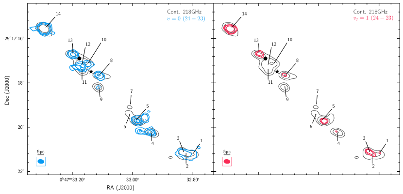
Figure 1: Grey contours show the $218$ GHz continuum emission. On the left panel the HC₃N $v=0$ $J=24-23$ integrated line emission contours are overlaid in blue. On the right panel the HC₃N^∗ $v_{7}=1$ $J=24-23$ integrated line emission contours are overlaid in red. All contours represent the $3\sigma$, $7\sigma$ and $15\sigma$ levels. The black circle indicates the position of TH2, $(\alpha(J2000),\delta(J2000))=(00^{\text{h}}47^{\text{m}}33^{\text{s}}.179,-25^{\circ}17^{\prime}17.13^{\prime\prime})$, (strongest compact radio source Ulvestad & Antonucci, 1997) and the black star the kinematic center as indicated by Müller-Sánchez et al. (2010). The beam size ($0.19^{\prime\prime}\times 0.29^{\prime\prime}$) is indicated on the lower left corner of the panels.

Table 3: MADCUBA fitted emission in Jy beam^-1 km s^-1 for HC₃N and HC₃N^∗ lines used for the analysis. The table also lists the transition frequency in GHz, the $J$ levels implied and the energy of the lower level ($E_{LO}$). Transitions with same $J$ numbers from a same vibrational level but different frequency come from the $l$-splitting of the vibrational levels due to the interaction between the angular momentum of the vibrationally excited states and the rotational angular momentum of the molecule (Goldsmith et al., 1983).

	V${}_{\text{LSR}}$	FWHM	v=0	v=0	$v_{7}=1$	$v_{7}=1\textsuperscript{a}$	$v_{6}=1$	$v_{6}=1$	$v_{7}=2$	$v_{7}=2$	$v_{7}=2$	$v_{7}=2$	$v_{7}=2$	$v_{7}=2$
$J\rightarrow J-1$	$(\text{km}$ $\text{s}^{-1})$	$(\text{km}$ $\text{s}^{-1})$	24-23	39-38	24-23	39-38	24-23	39-38	24-23	24-23	24-23	32-31	32-31	32-31
$l$-doubling					$(+1,-1)$	$(+1,-1)$	$(-1,+1)$	$(+1,-1)$	$(+2,-2)$	$(-2,+2)$	$(0,0)$	$(+2,-2)$	$(-2,+2)$	$(0,0)$
$\nu$ (GHz)			218.32	354.70	219.17	355.57	218.68	355.28	219.74	219.71	219.68	292.99	292.91	292.83
$E_{LO}$ (K)			120.50	323.48	441.81	645.11	838.35	1041.67	766.22	766.21	762.93	862.89	862.86	859.56
1	$310\pm 1$	$22\pm 4$	$0.18$	$0.13$	$0.07$	$0.10$	$\leqslant 0.05$	$0.06$	$-$	$-$	$-$	$-$	$-$	$-$
2	$307\pm 1$	$25\pm 2$	$0.33$	$0.23$	$0.14$	$0.31$	$0.08$	$0.19$	$\leqslant 0.05$	$\leqslant 0.05$	$\leqslant 0.05$	$0.08$	$0.08$	$0.08$
3	$299\pm 1$	$28\pm 2$	$0.38$	$0.28$	$0.17$	$0.22$	$0.12$	$0.11$	$\leqslant 0.05$	$\leqslant 0.05$	$\leqslant 0.05$	$0.09$	$0.11$	$0.11$
4	$253\pm 1$	$25\pm 3$	$0.37$	$0.28$	$0.12$	$0.15$	$0.08$	$0.10$	$\leqslant 0.05$	$\leqslant 0.05$	$\leqslant 0.05$	$0.09$	$0.08$	$0.06$
5	$212\pm 1$	$43\pm 2$	$0.76$	$0.81$	$0.21$	$0.29$	$0.13$	$0.17$	$\leqslant 0.07$	$\leqslant 0.07$	$\leqslant 0.07$	$0.21$	$0.19$	$0.22$
6	$219\pm 2\textsuperscript{b}$	$38\textsuperscript{b}$	$\leqslant 0.06$	$\leqslant 0.05$	$-$	$-$	$-$	$-$	$-$	$-$	$-$	$-$	$-$	$-$
7	$252\pm 2\textsuperscript{b}$	$32\textsuperscript{b}$	$\leqslant 0.06$	$\leqslant 0.05$	$-$	$-$	$-$	$-$	$-$	$-$	$-$	$-$	$-$	$-$
8	$302\pm 2$	$26\pm 3$	$0.34$	$0.35$	$0.14$	$0.21$	$\leqslant 0.05$	$0.09$	$-$	$-$	$-$	$-$	$-$	$-$
9	$165\pm 2$	$36\pm 4$	$0.12$	$0.08$	$\leqslant 0.06$	$\leqslant 0.05$	$-$	$-$	$-$	$-$	$-$	$-$	$-$	$-$
10	$274\pm 1$	$25\pm 3$	$0.20$	$0.33\textsuperscript{c}$	$\leqslant 0.05$	$\leqslant 0.04$	$-$	$-$	$-$	$-$	$-$	$-$	$-$	$-$
11	$141\pm 1$	$41\pm 2$	$0.28$	$0.32$	$\leqslant 0.07$	$0.16$	$-$	$-$	$-$	$-$	$-$	$-$	$-$	$-$
12	$150\pm 1$	$46\pm 3$	$0.36$	$0.18$	$\leqslant 0.07$	$\leqslant 0.06$	$-$	$-$	$-$	$-$	$-$	$-$	$-$	$-$
13	$250\pm 1$	$31\pm 1$	$0.70$	$0.71$	$0.36$	$0.39$	$0.10$	$0.18$	$\leqslant 0.06$	$\leqslant 0.06$	$\leqslant 0.06$	$0.09$	$0.08$	$0.10$
14	$201\pm 6$	$51\pm 14$	$2.74$	$3.56$	$1.12$	$1.59$	$0.45$	$0.78$	$0.41$	$0.40$	$0.40$	$0.69$	$0.69$	$0.71$

• ^a This transition is contaminated with the $v_{6}=1$ $J=39-38$ $(-1,+1)$ transition. The listed values have been corrected from this contamination using MADCUBA.

• ^b Velocities and linewidths for sources with upper-limits in HC₃N $v=0$ were taken from CS and C¹⁸O lines.

• ^c Strongly blended with HCN.

3.1 Radiative and Collisional Excitation of HC₃N

HC₃N is a linear molecule with seven vibrational modes, four stretching modes ($v_{1}$, $v_{2}$, $v_{3}$, $v_{4}$) and three bending modes ($v_{5}$, $v_{6}$, $v_{7}$) (Uyemura et al., 1982; Wyrowski et al., 1999). It is an excellent probe of the physical properties of hot and dense regions in the MW (i.e. Hot Cores) where massive star formation is taking place. In the warm regions where the gas is shielded from the UV radiation, the abundance of HC₃N is expected to increase due to the evaporation of this molecules from grain mantles. Furthermore, its high dipole moment ($3.73$ Debye, DeLeon & Muenter, 1985) traces high densities of $n_{\text{H}_{2}}>10^{5}$ cm^-3. The vibrational levels of HC₃N^∗ with energies ranging between $\sim 300$ K and $\sim 1000$ K above the ground state for the bending modes and above $3000$ K for the stretching modes are predominantly excited by warm $>200$ K mid-IR radiation. The $v_{7}=1$ and $v_{6}=1$ states can be excited via absorption of $45$ and $20$ $\mu$m photons, respectively, and could also be pumped via collisions with H₂ in hot and dense regions; however, the latter mechanism is restricted to small regions while the former is expected to be more efficient at the spatial scales probed by our observations. Since the Spectral Energy Distribution (SED) of the dust emission in regions with hidden massive star formation usually peaks in the $10-60$ $\mu$m region, it is expected that bending modes will be more easily excited than stretching modes, which require IR radiation at $5$ $\mu$m.

As a consequence of the high column densities, the extinction in star forming regions is very high, preventing the direct observation of the hot dust in the mid-IR. However, the HC₃N rotational transitions from its ground and vibrationally excited states are emitted in the (sub)millimeter range which is basically unaffected by dust extinction (even in extremely obscured objects like the nuclei of the ultraluminous IR galaxy Arp 220, Barcos-Muñoz et al., 2015; Martín et al., 2016), allowing to probe deeply embedded sources. Therefore, measuring multiple rotational transitions from different vibrational states of HC₃N provides a unique tool to infer their physical properties, their thermal and density structures, and the kinematics of the material heated by the protostars. Since the continuum optical depth in the mid-IR is expected to be high, the HC₃N molecules will be bathed by a blackbody at the local T${}_{\text{dust}}$, and the upper vibrational levels will be populated accordingly.

The typical densities of the HCs in the MW (few $10^{6}-10^{7}$ cm^-3) (Wyrowski et al., 1999; de Vicente et al., 2000) are usually much smaller than the critical densities ($n_{\text{cr}}$) required to collisionally excite the vibrational levels from the ground state. Values for $n_{\text{cr}}$ at $T=300$ K are of $4\times 10^{8}$ and $3\times 10^{11}$ cm^-3 for the excitation of the $v_{7}=1$ and $v_{6}=1$ states , respectively (Wyrowski et al., 1999), indicating that the excitation of the vibrational levels is usually dominated by radiation pumping in the mid-IR. Therefore, the detection of the rotational transitions from vibrationally excited levels can be used to infer the temperature of the warm dust. By contrast, collisions with H₂ may dominate the excitation of the rotational levels within the $v=0$, $v_{6}=1$, and $v_{7}=1$ vibrational states; the critical densities at $300$ K to excite the $J=24-23$ and $J=39-38$ transitions are of $2\times 10^{6}$ and $5\times 10^{6}$ cm^-3, respectively. While radiative pumping of the excited vibrational states and subsequent relaxation can potentially contribute to the rotational excitation, direct excitation through collisions will efficiently populate the rotational ladder within $v=0$, from which the excited vibrational states will be radiatively pumped. In summary, one expects a combination of collisional excitation of the rotational transitions within the vibrational state of HC₃N and radiative pumping for the the vibrational excitation.

4 Results

4.1 LTE modelling. Rotational and vibrational temperatures

As discussed in the previous section, the excitation of the HC₃N lines is dominated by different mechanisms: collisional for rotational transitions and IR pumping for vibrational transitions. To establish if the excitation of HC₃N is described by the Local Thermodynamic Equilibrium (LTE) with a single excitation temperature we have used two LTE analysis: the rotational diagram and the MADCUBA SLIM tool (Martín et al., 2019). On the one hand, the rotational diagrams simply assume optically thin emission. On the other hand, SLIM includes line optical depth effects by fitting not only the line ratios but also the absolute line fluxes and profiles with an assumed size for the source. For both analysis, we have first combined the relative intensities and line profiles of a given rotational transition ($J=24-23$, $J=32-31$ or $J=39-38$) arising from the ground state and the different vibrationally excited states to derive the excitation temperature between vibrational levels (hereafter the vibrational temperature, $T_{\text{vib}}$). The lines used to derive $T_{\text{vib}}$ cover a wide range of lower level energies, from $120$ K to $1041$ K for sources with detections of the $v_{6}=1$ lines; and to $645$ K for sources with detections of only the $v_{7}=1$ lines. Then, we have combined all the rotational transitions arising from the same vibrationally states (ground state, $v_{7}=1$, $v_{7}=2$ and $v_{6}=1$) to derive the excitation temperature of the rotational levels within the different vibrational states (hereafter the rotational temperature, $T_{\text{rot}}$).

4.1.1 Rotational diagrams

Figure 2 shows the LTE results for SHC14, the most prominent condensation, by combining all detected rotational lines in the different vibrational states to infer both $T_{\text{rot}}$ and $T_{\text{vib}}$. The rotational diagram (Fig. 2) clearly illustrates the presence of two different excitation temperatures, $T_{\text{vib}}$ of $363\pm 79$ and $445\pm 145$ K shown in blue and red solid lines respectively, derived from the $J=24-23$ and $J=39-38$ transitions in different vibrational levels, and the $T_{\text{rot}}$ of $107\pm 22$, $112\pm 24$, $116\pm 61$ and $125\pm 45$ K shown by dotted lines derived from the different rotational transitions arising from the same vibrational state. The rotational diagram clearly illustrates that $T_{\text{vib}}$ and $T_{\text{rot}}$ have quite different values of $\sim 400$ and $\sim 110$ K, respectively.

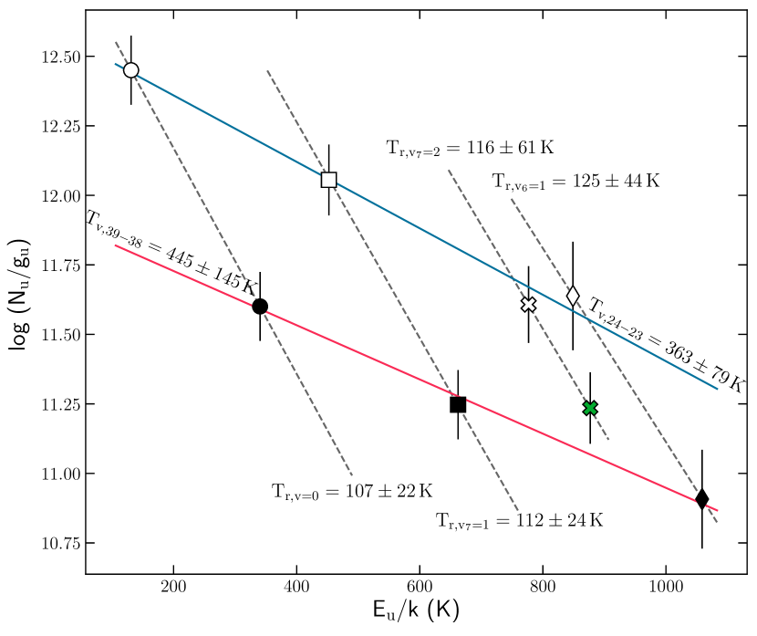
Figure 2: Rotational diagram derived from the line intensities of HC₃N^∗ for source $14$. The data from the $J=24-23$ and $J=39-38$ transition are indicated by empty and filled markers, respectively. The green colored cross represents the $J=32-31$ transition from $v_{7}=2$. The population levels arising from different vibrational states $v=0$, $v_{7}=1$, $v_{7}=2$ and $v_{6}=1$ are represented as circles, squares, crosses and diamonds. The blue and red solid lines represent the fit to the $J=24-23$ and the $J=39-28$ transitions, respectively. The dotted lines represent the fit to same vibrational state transitions. The temperatures derived from each fit are indicated.

4.1.2 SLIM analysis

In addition to the rotational diagram analysis, the observed HC₃N line profiles from the ground and vibrationally excited levels have been fitted using the SLIM tool to derive the physical properties of the sources with HC₃N emission. SLIM simulates all lines profiles and intensities emitted under LTE conditions including line optical depth effects for a given source size. The SLIM LTE analysis considers, as free parameters, the column density ($N$) of HC₃N, the excitation temperature ($T_{\text{vib}}$ or $T_{\text{rot}}$ depending on the transitions considered), the radial velocity ($V_{\text{LSR}}$), the linewidth and the size of the emitting source (defined as FWHM, full width at half maximum). Since the HC₃N^∗ sources are unresolved by our beam of $0.2^{\prime\prime}$, we have adopted an upper limit to their sizes of $0.1^{\prime\prime}$, i.e. half of the beam size. Therefore the inferred column densities could be lower limits if the source sizes are substantially smaller than the assumed value, nonetheless the derived excitation temperatures remain independent of this choice.

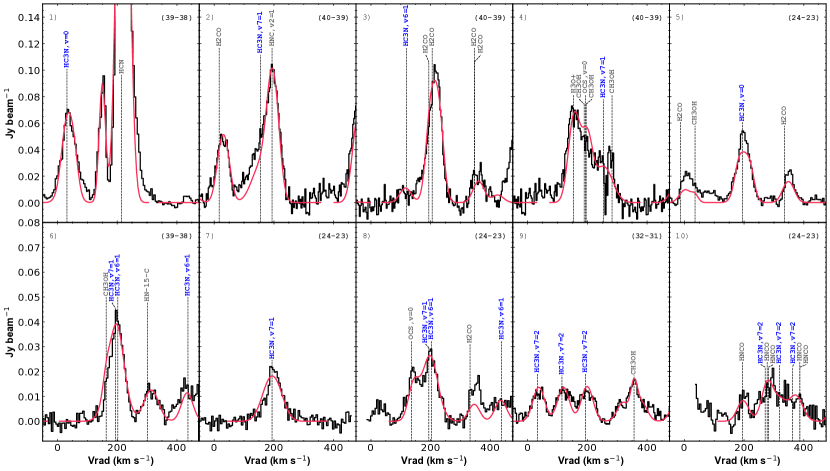
Figure 3: Observed spectra (black histograms) towards source $14$. HC₃N lines from the ground and vibrational states $v_{7}=1$, $v_{7}=2$, and $v_{6}=1$ are marked in blue. On the top-right corner of each panel the ($J$, $J-1$) of the HC₃N transitions present in that panel is indicated. The red solid lines represent the fitted model from the LTE analysis obtained with MADCUBA.

Figure 3 shows the SLIM predictions of the line profiles for all HC₃N^∗ lines detected in SHC14 in red solid line superimposed on the observed spectra. We have used the AUTOFIT tool in SLIM, which performs a non-linear least squared fit of the LTE line profiles to the data using the Levenberg-Marquartd algorithm. Since SLIM uses the partition function given by the CDMS catalog, which only uses the ground vibrational state to derive the partition function, we have corrected the estimated column densities by calculating the total partition function, including all rotational levels inside the ground state and vibrationally excited states ($v_{7}=1$, $v_{6}=1$ and $v_{7}=2$). The corrected column densities and temperatures derived from our LTE SLIM model fitting for all sources are summarized in Table 4. The inferred temperatures are in general agreement with those derived via the rotational diagram method.

The inferred $T_{\text{vib}}$ by the two methods (SLIM and rotational diagram) are high, ranging from $\sim 216$ K to $\sim 393$ K for sources with at least one of the $v_{7}=1$ lines detected above the $3\sigma$ level (sources $1$, $2$, $3$, $4$, $5$, $8$, $13$ and $14$). It is interesting to note that the $T_{\text{rot}}$ within a given vibrational level does not vary significantly among different sources. However, there is a trend for $T_{\text{rot}}$ to increase with the energy of the vibrational level. The average rotational temperatures are: $T_{\text{rot}}=91$ K for $v=0$, $T_{\text{rot}}=152$ K for $v_{7}=1$ and $T_{\text{rot}}=206$ K for $v_{6}=1$. This is clear indication that in the case of collisional excitation of the rotational lines, the regions where the $v_{6}$ rotational transitions arise have larger H₂ densities (and kinetic temperatures) than those arising from the ground and the $v_{7}$ vibrational levels. This could imply the presence of density and temperature gradients in the structure of the SHCs (de Vicente et al., 2000), as expected if they are associated with very recent star formation in the cloud.

We have also derived upper limits to $T_{\text{vib}}$ of $\sim 100-160$ K for the massive star forming regions $9$, $10$, $11$ and $12$, where no vibrationally excited lines were detected. As discussed in Section 6, these sources (along with sources $6$ and $7$) likely represent a more evolved stage in the evolution of the formation of SSCs.

The differences found between the vibrational and rotational temperatures ($T_{\text{vib}}\gg T_{\text{rot}}$) and between the $T_{\text{rot}}$ for distinct vibrational states (see Figs. 3 and 2 and Table 4), clearly suggests that the HC₃N^∗ excitation is not in LTE as expected when the H₂ density is not high enough to thermalize the population of the rotational levels.

Table 4: Derived parameters for the SSCs in NGC 253 from the SLIM LTE modelling assuming a source size of $0.1^{\prime\prime}$. Column densities have been corrected by including the contribution from the vibrational states into the partition function. Column density errors are indicated in parenthesis. For SSCs without a T${}_{\text{rot}}$ estimation for $v_{7}=1$, a fiducial T${}_{\text{rot}}=100$ K was assumed to get an HC₃N column density upper limit.

SSC		log N(HC3N)a	T${}_{\text{vib}}$	T${}_{\text{rot}}$
				v=0	$v_{7}=1$	$v_{6}=1$
		(cm-2)	(K)	(K)	(K)	(K)
1	SHC	$16.3(15.4)$	$216\pm 15$	$84\pm 9$	$132\pm 3$	$259\pm 19$
2	SHC	$16.4(15.2)$	$304\pm 70$	$69\pm 6$	$170\pm 4$	$227\pm 5$
3	SHC	$16.2(15.9)$	$337\pm 50$	$78\pm 4$	$162\pm 36$	$240\pm 15$
4	SHC	$16.4(16.2)$	$326\pm 52$	$93\pm 6$	$142\pm 25$	$193\pm 13$
5	SHC	$16.6(15.5)$	$269\pm 22$	$110\pm 5$	$160\pm 35$	$130\pm 12$
6		$\leqslant 14.6$	$-$	$100$	$-$	$-$
7		$\leqslant 14.6$	$-$	$100$	$-$	$-$
8	SHC	$16.1(15.1)$	$217\pm 14$	$102\pm 16$	$165\pm 45$	$\sim 181$
9		$\leqslant 16.2$	$\leqslant 126$	$\leqslant 88$	$-$	$-$
10		$\leqslant 16.0$	$\leqslant 132$	$\leqslant 84$	$-$	$-$
11		$\leqslant 15.9$	$\leqslant 165$	$113\pm 10$	$\leqslant 138$	$-$
12		$\leqslant 16.1$	$\leqslant 140$	$76\pm 6$	$-$	$-$
13	SHC	$16.8(16.3)$	$393\pm 34$	$104\pm 4$	$159\pm 21$	$206\pm 8$
14	SHC	$17.6(16.6)$	$312\pm 20$	$96\pm 13$	$139\pm 12$	$124\pm 29$

• ^a $\log{N}=a(b)$ represent $N=10^{a}\pm 10^{b}$.

4.2 Non-LTE modelling

To properly account for the different excitation mechanisms of the vibrational and rotational transitions of HC₃N, we have carried out non-LTE radiative transfer modelling of HC₃N, considering both the effects of the mid-IR radiation from the warm dust and the collisional excitation. We have used the radiative transfer code described in González-Alfonso & Cernicharo (1997, 1999) to calculate the statistical equilibrium populations arising from a uniform spherical cloud.

In our model, we have included the HC₃N rotational transitions up to $J=45$ in the $v=0$, $v_{7}=1$ and $v_{6}=1$ vibrational states. Since collisional rates with H₂ for the transitions from the ground to vibrationally excited levels are not available, we have estimated them following the approach described by Deguchi et al. (1979), Goldsmith et al. (1982) and Wyrowski et al. (1999). We have also assumed the same collisional rates for the excitation of the rotational levels by para- and ortho-H₂ for the $v=0$, $v_{7}=1$ and the $v_{6}=1$ states (taken from Faure et al., 2016), and considered that there are no propensity rules for the $l$-type doubling: $C_{v_{7},v_{6}}(J_{\text{up}},l_{\text{up}}\rightarrow J_{\text{low}},l_{\text{low}})=0.5C_{v0}(J_{\text{up}},J_{\text{low}})$. Here $C_{v_{7},v_{6}}$ and $C_{v0}$ are the collisional rates for a rotational transition in the vibrational level $v_{7}=1$ or $v_{6}=1$ and in the ground state, respectively.

For a given dust temperature ($T_{\text{dust}}$) and a dust column density, the model calculates the radiation field from the mid-IR to millimeter wavelengths within a uniform spherical cloud. This radiation field is used to radiatively pump the rotational levels in the $v_{7}=1$ and $v_{6}=1$ vibrationally excited states. The model also returns the SED of the dust emission (i.e a grey body) emerging from the spherical cloud, which is integrated to determine the total luminosity. In addition to the radiative excitation dominated by the dust, the model also calculates the collisional excitation of HC₃N for a given H₂ density assuming that the gas kinetic temperature is equal to the dust temperature. This assumption is justified by the relatively large H₂ densities of $\sim 10^{6}$ cm^-2 derived from our LTE modelling (see Section 4), for which both temperatures should be closely coupled, as seen in MW HCs (de Vicente et al., 2000). For the line radiation transfer, the model assumes a Gaussian line profile with the linewidth as a free parameter. We have used the model to predict the HC₃N emission for the rotational lines from the $v_{6}=1$, $v_{7}=1$ and $v=0$ vibrational states as a function of the H₂ density, the dust/kinetic temperature, the HC₃N column density and the dust column density parameterized by the dust opacity at $100$ $\mu$m, $\tau_{100}$. The $\tau_{100}$ can be transformed into the gas H₂ column density for a gas-to-dust ratio of $100$ by

$$N(\text{H}_{2})=6.5\times 10^{23}\tau_{100}\,(\text{cm}^{-2})$$ (1)

where the mass absorption coefficient of dust at $100$ $\mu$m has been taken to be $44.5$ $\text{cm}^{2}\text{g}^{-1}$ (González-Alfonso et al., 2014) with a dust emissivity index of $1.6$.

The predictions of our non-LTE modelling for a spherical cloud with uniform density and dust/kinetic temperature are summarized in Fig. 4. This figure shows the predicted intensity ratio between the rotational transition, $J=24-23$, from the vibrational levels $v=0$ and $v_{7}=1$ (hereafter $v_{0}/v_{7}$ ratio) plotted against the predicted intensity ratio between two rotational transitions $J=39-38$ and $J=24-23$ from the ground state $v=0$ ($v_{0}$ ratio) on the left panel, the vibrational state $v_{7}=1$ ($v_{7}$ ratio) on the middle panel and the vibrational state $v_{6}=1$ ($v_{6}$ ratio) on the right panel. The continuum optical depth at $100$ $\mu$m, $\tau_{100}$, has been varied from $4$ in the upper panels to $16$ in the lower panels, covering the relevant H₂ gas column densities from $2.5\times 10^{24}$ to $1.0\times 10^{25}$ cm^-2. The colored solid lines in all panels indicate the dependence of the line intensity ratios on H₂ densities and the reddish contour levels show the dependence of the line ratios on the dust/kinetic temperature. For Figure 4 a representative HC₃N column density of $5\times 10^{16}$ cm^-2 was assumed (solid lines), however, to show the dependency on the HC₃N column density (i.e. the HC₃N abundance), we have shaded the regions that cover a column density varying from $5\times 10^{16}$ cm^-2 (solid lines) to $1\times 10^{17}$ cm^-2 (dashed lines) for two different H₂ densities: $1.0\times 10^{6}$ and $2.5\times 10^{6}$ cm^-3 (blue and cyan shaded regions). These HC₃N column densities ($5\times 10^{16}$ cm^-2 and $1\times 10^{17}$ cm^-2) translate into HC₃N abundances ranging from $X$(HC₃N)$=4\times 10^{-9}$ to $2\times 10^{-8}$.

Figure 4 clearly shows the expected trends for the different line ratios. The vibrational $v_{0}/v_{7}$ ratio is extremely sensitive to the dust temperature with the iso-contours of $T_{\text{dust}}$ running basically horizontally. The $v_{0}$, $v_{7}$ and $v_{6}$ line ratios show a nearly linear dependence with $n_{\text{H}_{2}}$ density (colored lines) with iso-density lines running from upper-left to the bottom-right, with density increasing from left to right (H₂ densities corresponding to each color are indicated on the horizontal color bar). On the other hand, the line ratios have a weak dependence on the HC₃N abundance/column density as shown with the dashed lines, although this dependence increases as the density increases. Finally, the dust opacity has a weak effect on the derived dust temperature and a moderate effect on the derived H₂ densities. For a given vibrational ratio $v_{0}/v_{7}$, an increase of the dust opacity by a factor of $4$ requires increasing the dust temperature by just only a factor of $\sim 1.2$ and the H₂ density by less than a factor of $2$.

In Figure 4 we have included, as open circles, the observed ratios from all sources (labelled by their number). The sources with no detection of $v_{7}=1$ lines (condensations $9$, $10$, $11$ and $12$), only appear in the left-hand panels as lower limits for the $v_{0}/v_{7}$ ratio.

Table 5 shows the estimated parameters from the best fit to the non-LTE models together with their associated errors. Given the number of free parameters in our non-LTTE modelling, selecting the model parameters that best-fit our data and estimating the error is not straightforward. Fortunately, as illustrated in Fig. 4, the range of model parameters that can account for the observed line ratios is relatively narrow. Dust temperatures range from $200$ to $400$ K, in good agreement with the LTE modelling, and densities are between $10^{6}$ and $10^{7}$ cm^-3, with a systematic trend to lower densities when only the $v_{0}$ $J=39-38/J=24-23$ ratio is considered. The non-LTE parameters that “best fit” the data and their uncertainties have been derived from the parameter space of all models that fit the observed line intensity ratios within a given uncertainty of the observed ratio. For every SHC, we have extracted the set of model parameters that fit, within $\pm 20\%$, the observed $v_{7}$ line ratios. Then we have derived the best fit parameter as the average of the set of parameters weighted according to a Gaussian distribution. The errors shown in Table 5 correspond to the sigma value of the weighted average.

As previously mentioned, the inferred H₂ densities are very similar for all sources. However, the H₂ densities derived only from the $v_{7}=1$ rotational lines are systematically larger than those from the ground state by a factor of $\sim 1-5$, indicating the presence of density gradients in the SHCs. The non-LTE results from Fig. 4 shows that the H₂ densities are only weakly dependent on the kinetic temperature, $T_{\text{kin}}\sim T_{\text{dust}}$. Therefore, we have also derived the H₂ densities for sources $9$, $10$, $11$ and $12$, which are also included Table 5, and they are shown Fig. 4 by black arrows. The H₂ densities were derived from the measured line ratios of the rotational transitions in the ground vibrational state assuming a kinetic temperature close to the upper limit to T${}_{\text{vib}}$ derived from LTE. It is remarkable that their H₂ densities are similar to those of the SHCs but with lower kinetic temperatures.

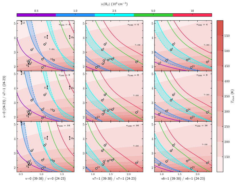
Figure 4: HC₃N non-LTE modelling results summarized as the line intensity ratio between the rotational transition $J=24-23$ from the vibrational state $v=0$ and $v_{7}=1$ versus the line intensity ratio between the $J=39-38$ and the $J=24-23$ rotational transition from the ground state $v=0$ (left panels) and from the vibrational states $v_{7}=1$ (middle panels) and $v_{6}=1$ (right panels). Red contours indicate dust/kinetic temperatures, ranging from $100$ K to $600$ K. Colored solid lines indicate the model dependence with density for an HC₃N column density of $5\times 10^{16}$ cm^-2. The H₂ density corresponding to each color is indicated on the horizontal colorbar. The colored shaded regions show the effect of varying the HC₃N column density from $5\times 10^{16}$ cm^-2 (solid lines) to $10^{17}$ cm^-2 (dashed lines) on models with H₂ densities of $1\times 10^{6}$ (blue) and $2.5\times 10^{6}$ cm${-3}$ (cyan). The top, center and bottom panels show the results for dust opacities $\tau_{100}=4$, $8$ and $16$, respectively. These values translate into $N(\text{H}_{2})=2.6\times 10^{24}$, $5.2\times 10^{24}$ and $1.04\times 10^{25}$ cm^-2 for the top, middle and bottom panels. The observed ratios for the SHCs are shown with filled black white circles and sources without the detection of $v_{7}=1$ lines are represented with black arrows only in the left panel.

Table 5: Derived physical parameters for the SSCs in NGC 253 from LTE analysis and non-LTE modelling. Sizes are derived from $v_{7}=1$ ($v=0$ for sources in which $v_{7}=1$ transitions are upper limits, marked with ^∗) assuming it is optically thick and thus represent lower limits.

SSC	Type	Size	$n_{H_{2}}$	$M_{H_{2}}$	T${}_{\text{vib}}$	T${}_{\text{kin}}$	L${}_{\text{app}}\textsuperscript{a}$	L${}_{\text{app}}\textsuperscript{b}$
		(mas)	($10^{6}$ cm-3)	($10^{3}$ M⊙)	(K)	(K)	($10^{8}$ L⊙)	($10^{8}$ L⊙)
			non-LTE	non-LTE	LTE	non-LTE	LTE	non-LTE
1	SHC	$20$	$1.9\pm 0.4$	$2.0\pm 0.4$	$216\pm 15$	$285\pm 58$	$1.1\pm 0.3$	$2.3\pm 1.4$
2	SHC	$22$	$6.0\pm 2.0$	$8.0\pm 2.7$	$304\pm 70$	$322\pm 64$	$5.2\pm 4.8$	$4.4\pm 2.5$
3	SHC	$22$	$1.6\pm 0.6$	$2.1\pm 0.8$	$337\pm 50$	$324\pm 76$	$7.9\pm 4.6$	$4.6\pm 2.9$
4	SHC	$19$	$3.3\pm 1.8$	$3.0\pm 1.7$	$326\pm 52$	$191\pm 34$	$5.3\pm 3.4$	$1.1\pm 0.4$
5	SHC	$22$	$4.5\pm 1.9$	$5.7\pm 2.6$	$269\pm 22$	$189\pm 37$	$3.1\pm 1.0$	$0.5\pm 0.6$
8	SHC	$25$	$3.4\pm 1.6$	$6.8\pm 3.2$	$217\pm 14$	$263\pm 38$	$1.8\pm 0.5$	$3.5\pm 1.4$
9∗		$26$	$0.9\pm 0.1$	$0.6\pm 0.1$	$\leqslant 126$	$\leqslant 129$	$\leqslant 0.2$	$\leqslant 0.09$
10∗		$39$	$10\pm 3.3$	$3.4\pm 1.2$	$\leqslant 132$	$\leqslant 118$	$\leqslant 0.6$	$\leqslant 0.06$
11∗		$36$	$1.9\pm 0.7$	$2.1\pm 0.8$	$\leqslant 165$	$\leqslant 188$	$\leqslant 0.5$	$\leqslant 0.27$
12∗		$39$	$1.0\pm 0.4$	$0.9\pm 0.2$	$\leqslant 140$	$\leqslant 125$	$\leqslant 0.6$	$\leqslant 0.13$
13	SHC	$27$	$1.6\pm 0.2$	$2.7\pm 0.6$	$393\pm 34$	$382\pm 42$	$23\pm 8$	$10\pm 3$
14	SHC	$42$	$2.3\pm 0.5$	$22\pm 4$	$312\pm 20$	$271\pm 47$	$22\pm 6$	$10\pm 4$

• ^a Luminosities obtained assuming a black body emitting at the T${}_{\text{vib}}$ derived from LTE modelling (i.e. $L=4\pi r^{2}\sigma T_{\text{vib}}^{4}$).

• ^b Luminosities obtained by integrating the predicted SED from the non-LTE models between $10$-$1200$ $\mu$m.

5 Derived properties

5.1 Sizes, HC₃N abundances and masses

As already mentioned, since none of the detected SHCs are spatially resolved, we can set up an upper limit to their sizes of $0.1^{\prime\prime}$ ($<1.7$ pc). In addition, we can also estimate a lower limit to the SHCs sizes by assuming that the rotational transitions within the $v_{7}=1$ state are optically thick and therefore the source brightness temperature will be the vibrational temperature derived from the LTE analysis. From the ratio of the observed and expected line intensities for the optically thick case and assuming a Gaussian source, we have estimated the lower limit to the sizes shown in Table 5. The lower limits range from $43$ to $14$ milliarcseconds (mas), which translate to $0.72$ and $0.24$ pc. These lower limits are factors $2-7$ smaller than the upper limit to the size of $0.1^{\prime\prime}$.

Combining the HC₃N column densities derived from the LTE analysis with the H₂ densities estimated from non-LTE modelling and the lower limits to their sizes, we can estimate the H₂ column densities, the fractional abundances of HC₃N, $X(\text{HC}_{3}\text{N})=N(\text{HC}_{3}\text{N})/N(H_{2})$, and the masses of the forming SSCs. The estimated H₂ columns densities range from $3-9\times 10^{24}$ cm^-2 and $X(\text{HC}_{3}\text{N})\sim 10^{-9}$, similar to the HCs found in our galaxy ( $5\times 10^{-9}$ for Sgr B2M and Sgr B2N2, $5\times 10^{-9}$ for Orion KL HC, from de Vicente et al., 2000, 2002). From the H₂ column densities (N${}_{\text{H}_{2}}$) and the H₂ densities derived from the non-LTE modelling we can estimate the depth of the emission along the line of sight. This depth, when compared to the estimated size, provides information on how the emitting regions are distributed along the line of sight. The mean value of the inferred depths is $0.89$ pc, just within the lower and upper limits to the sizes, suggesting a nearly spherical distribution.

The H₂ masses of the SHCs in Table 5 range from a few $10^{3}$ M_⊙ to a few $10^{4}$ M_⊙. However, the estimated masses from the models must be considered with caution since they are lower limits as they have been derived from the lower limit to the sizes. Nevertheless, the SHC masses derived from the HC₃N^∗ emission only represent the hot inner core of the larger condensations observed by Leroy et al. (2018) in the $350$ GHz continuum emission. Therefore, the M${}_{\text{gas}}$ in Table 6 is always larger than M${}_{\text{H}_{2}}$ in Table 5, by up to a factor of $10$.

To derive the lower limit to the sizes of sources with no detection of HC₃N^∗, we have used the same procedure as for SHCs, but using the line intensity of the rotational lines from the ground vibrational state and assuming a $T_{\text{kin}}$ of $130$ K. The lower limits to the masses and the sizes are very similar to those derived for the SHCs.

5.2 SSCs luminosities

5.2.1 “Apparent” luminosities

From the estimated H₂ column densities from non-LTE modelling, the dust opacity in the mid-IR (the wavelength range responsible for the vibrational excitation of HC₃N) is larger than $20$ at $40$ $\mu$m. Therefore, SHCs will emit as a black body at the temperature of the far-IR photosphere. A strong upper limit to the luminosity, which will be denoted as the apparent luminosity ($L_{\text{app}}$), can be obtained by adopting a temperature $T_{\text{vib}}$ for the photosphere, as derived from the LTE analysis. The same approach has been carried for the SSCs with only HC₃N^∗ detection as upper limits. The derived $L_{\text{app}}$ from LTE modelling are shown in Table 5. In addition to the LTE estimates of the apparent luminosities, an alternative $L_{\text{app}}$ is also estimated from the integration between $10$ and $1200$ $\mu$m of the non-LTE modelling predicted SED (Table 5). Both luminosities must be considered as lower limits since they were obtained by assuming the lower limit source sizes as derived from HC₃N^∗ emission. Similar apparent luminosities and trends are found for both LTE and non-LTE apparent luminosities. The difference between the apparent luminosities calculated from LTE and non-LTE, apart from the somewhat different vibrational/kinetic temperatures, arises from the fact that the LTE luminosity is from a black body and the non-LTE luminosity is calculated from a grey body, i.e. a factor $\sim 1.6$ between both luminosities.

5.2.2 Protostar luminosities

In the previous section we have made estimates of a lower limit to the SSCs apparent luminosities from the observed parameters. However, to estimate the actual luminosities of the heating sources is not straightforward. In fact, the estimated $L_{\text{app}}$ only represents the actual luminosity in the case of low dust column densities, i.e H₂ column densities of $<10^{23}$ cm^-2. For larger column densities, the derived $L_{\text{app}}$ should be considered an upper limit to the actual luminosity. This is due to the back-warming or greenhouse effect, first described by Donnison & Williams (1976) and more recently by González-Alfonso & Sakamoto (2019). The back-warming occurs when a fraction of the IR radiation from the heating source absorbed in an optically thick dust shell of the SHCs returns to the source due to the re-emission of the IR radiation by the inner surfaces of the shell. Then the thermal equilibrium at the inner surface is achieved for larger dust temperatures than those expected in the optically thin case. Therefore, the luminosity derived from the measured dust temperature at a given radius overestimates the actual luminosity of the heating source. For the large H₂ column densities found in the forming SSCs ($>10^{24}$ cm^-2) this effect needs to be taken into account to derive the luminosities of sources heating the SSCs.

Ivezic & Elitzur (1997) have made an estimate of the back-warming effect by using self-similarity and the scaling method for a centrally heated spherical cloud for different density profiles. Following this method we can estimate the actual luminosity arising from the protostars in the SSCs ($\text{L}_{\text{p}^{*}}$) can be inferred from $L_{\text{app}}$ by using equation $14$ of Ivezic & Elitzur (1997) as:

$$L_{\text{p}^{*}}=\frac{4}{\psi}L_{\text{app}}$$ (2)

where $\psi$ is a complex function of the total column density and the radial density profile of the cloud, and of the emissivity properties of the dust. Since $\psi$ is a very strong function of the radial density profile, a precise estimate of the luminosity of the heating sources from the measured $L_{\text{app}}$ requires knowledge of the density gradient. Taking a representative H₂ column density of a few $10^{24}$ cm^-2, as derived from the H₂ densities and the lower limit to the sizes, and considering that a HC typical density profile lies between $1$ and $2$, we estimate the factor $4/\psi$ to be roughly of $1/10$. Consequently, in the following discussions we will consider the luminosity of the heating sources of the SSCs, $\text{L}_{\text{p}^{*}}$, to be around one order of magnitude smaller than the $\text{L}_{\text{app}}$ from Table 5 ($\text{L}_{\text{app}}$ from the non-LTE modelling for SSCs with SHCs and from LTE modelling for the remaining SSCs). The rough estimated luminosities $\text{L}_{\text{p}^{*}}$ associated to the protostars heating the SSCs are shown in Table 6. Taking into account that the luminosities have been derived from lower limit source sizes, they are likely to represent a lower limit to the actual luminosity. Considering the size derived from the depth of the emission (see Section 5.1), $\text{L}_{\text{app}}$ will be larger by a factor of $\sim 4$, but the correction for the back-warming effect will also increase due to the larger H₂ column density. In this case the derived $\text{L}_{\text{p}^{*}}$ will be similar, within a factor of $2$, to the $\text{L}_{\text{p}^{*}}$ derived from the lower limit to the sizes.

Table 6: SSCs sizes, masses and luminosities. Protostar luminosities (L${}_{\text{p}^{*}}$) of condensations with no detection of $v_{7}=1$, marked with ^∗, have been calculated using T${}_{\text{rot}}$ from the ground state rotational transitions and assuming a source size derived from its emission. Sources marked with ^∗∗ show no HC₃N emission. Masses in form of protostars (M${}_{\text{p}^{*}}$) have been derived from L${}_{\text{p}^{*}}$ assuming a light-to-mass ratio of $10^{3}$ L${}_{\odot}/$M_⊙, similar to the value used for ZAMS massive stars.

	Sizes			Masses				Luminosities				SSC Phase
	SSC	Dust${}_{350\text{GHz}}\textsuperscript{a}$		M${}_{\text{gas}}$b	M${}_{\text{p}^{*}}$	M∗c		L${}_{\text{p}^{*}}$	L∗d	L${}_{\text{p}^{*}}$/L∗
	(pc)	(pc)		($10^{4}$ M⊙)	($10^{5}$ M⊙)	($10^{5}$ M⊙)		($10^{8}$ L⊙)	($10^{8}$ L⊙)
1	0.34	2.7		7.94	0.3	0.20		0.23	0.20	1.14		proto
2	0.37	1.2		5.01	0.4	0.20		0.44	0.20	2.22		proto
3	0.37	2.6		12.59	0.4	0.13		0.46	0.13	3.52		proto
4	0.33	2.5		12.59	0.1	1.00		0.11	1.00	0.11		proto
5	0.37	2.1		19.95	0.05	2.51		0.05	2.51	0.02		ZAMS
6	1.7∗∗	2.1		0.40		1.99			1.99			ZAMS
7	1.7∗∗	2.9		3.16		0.32			0.32			ZAMS
8	0.43	1.9		15.85	0.4	0.63		0.35	0.63	0.56		proto
9∗	0.44	2.6		5.01	0.02	3.16		0.02	3.16	$<0.01$		ZAMS
10∗	0.67	3.5		15.85	0.06	1.99		0.06	2.00	$<0.03$		ZAMS
11∗	0.62	2.9		3.16	0.05	3.98		0.05	3.98	$<0.01$		ZAMS
12∗	0.67	4.3		1.26	0.06	10.00		0.06	10.00	$<0.01$		ZAMS
13	0.46	1.6		15.85	1.0	0.63		1.02	0.63	1.62		proto
14	0.72	1.6		50.12	1.0	3.16		1.00	3.16	0.32		proto

• ^aLeroy et al. (2018) sizes derived from the dust continuum emission at $350$ GHz.

• ^bLeroy et al. (2018) gas mass estimates from $350$ GHz dust emission, assuming T${}_{\text{dust}}=130$ K and a dust-to-gas ratio of $0.01$.

• ^cLeroy et al. (2018) ZAMS stellar masses derived from L${}_{\text{p*}}$ assuming a light-to-mass ratio of $10^{3}$L${}_{\odot}/$M_⊙.

• ^dLeroy et al. (2018) derived luminosities from the $36$ GHz continuum emission assuming it is dominated by free-free emission.

6 Discussion

6.1 SHCs in NGC 253: Evolutionary earliest phases of Super Star Clusters

SSCs represent the most massive ($\text{M}_{*}\sim 10^{5}-10^{7}$ M_⊙) examples of clustered star formation. SSCs are compact, with radius $\sim 1-5$ pc, and young, $1-100$ Myr (Whitmore, 2002; Alonso-Herrero et al., 2003; Kornei & McCrady, 2009). Although SSCs are believed to be the precursors of Globular Clusters (GCs, with ages $\gtrsim 10$ Gyr), not all SSCs will evolve to a bound cluster as it requires a very high star formation efficiency (SFE) and high star formation rate (SFR) to prevent early disruption of the cocoon due to the feedback generated by high mass star formation (Hills, 1980; Beck, 2015; Johnson et al., 2015).

HCs are indeed expected to represent the earliest phases of massive star formation. HCs are internally heated by massive protostars deeply embedded in the parent molecular cloud, which is still undergoing gravitational collapse with mass accretion rates as high as a few $10^{-3}$M_⊙ yr^-1 (Walmsley, 1995). The consequent large concentration of gas and dust around protostars prevents the development of the Ultra-Compact H ii region (UCHII) (Walmsley, 1995; Churchwell, 2002; Hoare et al., 2007). The UCHII emerges when the accretion rate decreases below a threshold value. The flickering of the continuum emission observed in UCHII has been interpreted as due to the latest episodes of mass accretion onto UCHII regions (De Pree et al., 2014). Once the accretion stops, the UCHII region expands and evolves into an H ii region. The timescales for these processes are very short, from $\sim 10^{5}$ yr when the H ii region may start to show up, to a few $10^{6}$ yr, when SN explosions from the most massive stars will take place.

Our detection of HC₃N^∗ emission, indicative of extremely high column densities of gas and dust around the heating protostars, suggest that the condensations detected in the continuum by Leroy et al. (2018) represent indeed the earliest phases of SSCs evolution. In fact, some of them ($10$, $11$ and $13$) show strong Hydrogen recombination lines likely associated to H ii regions with a steep electron density profile (Báez-Rubio et al., 2018), as expected for extremely young UCHII regions (Jaffe & Martín-Pintado, 1999; Báez-Rubio et al., 2014). We have detected $8$ out of $14$ SSCs candidates in HC₃N^∗ (i.e. SHCs), indicative of a very early phase in their evolution.

Table 6 summarizes the main properties of the NGC 253 forming SSCs, their sizes, their stellar and gas content and their luminosities. The gas mass (M${}_{\text{gas}}$) of the SSCs, derived from the $350$ GHz dust continuum emission; the luminosities (L_∗) from ionizing Zero Age Main Sequence (ZAMS) stars, estimated from the $36$ GHz continuum emission assuming it is dominated by free-free emission; and the mass of ZAMS stars (M_∗), obtained from L_∗ by assuming a light-to-mass ratio of $10^{3}$ L${}_{\odot}/$M_⊙; have been taken from Leroy et al. (2018). The L_∗ and M_∗ values could be overestimated in some sources in the very central region (close to the brightest radio source TH2, Turner & Ho, 1985) due to the contribution of synchroton emission to the $36$ GHz continuum emission (Báez-Rubio et al., 2018). To complete the census of the star population in the forming SSCs, we have also added the luminosity in protostars, L${}_{\text{p*}}$ (i.e. the apparent luminosities from Table 5 corrected by an order of magnitude using Eq. 2). The estimated protostellar luminosities are typically of a few $10^{7}$ $\text{L}_{\odot}$ for most of the SHCs, with SHC13 and SHC14 reaching $10^{8}$ $\text{L}_{\odot}$. On the other hand, sources with HC₃N^∗ only detected as upper limits have estimated protostellar luminosities $\sim 10^{6}$ $\text{L}_{\odot}$, one order of magnitude smaller than the SHCs. The total luminosity (from proto and ZAMS stars) of all SSCs is $3.4\times 10^{9}$ $\text{L}_{\odot}$ (from which L${}_{\text{p*Total}}=4\times 10^{8}$ $\text{L}_{\odot}$ and L${}_{\text{*Total}}=30\times 10^{8}$), which accounts for about $22\%$ ($\sim 3\%$ from protostars and $\sim 19\%$ from ZAMS stars) of the total luminosity of the central region of NGC 253, assuming that half of the galaxy’s total luminosity, $3.1\times 10^{10}$ $\text{L}_{\odot}$, arises form the central $170$ pc (Melo et al., 2002; González-Alfonso et al., 2015). The remaining central luminosity of the galaxy would be produced by the star formation and more evolved SSCs outside the studied condensations (see Fig. 10) that occurred in the last $10$ Myr (Watson et al., 1996; Fernández-Ontiveros et al., 2009).

We have used the luminosity to make an estimate of the mass in protostars, M${}_{\text{p*}}$, by assuming a light-to-mass ratio of $10^{3}$ L_⊙ M${}_{\odot}^{-1}$. This is the same value used by Leroy et al. (2018) to derive the mass in ZAMS stars (M${}_{\text{*}}$). We used this value since the timescales for the massive protostars to reach the ZAMS are rather short and are expected to be close to the ZAMS evolutionary track (Hosokawa & Omukai, 2009). The assumed light-to-mass ratio is obviously uncertain since we do not know the SSC Initial Mass Function and the accretion rates. We have adopted the value corresponding to a representative cluster star of $10-20$ M_⊙ with a high accretion rate of a few $10^{-4}$ M_⊙ yr^-1. Our adopted light-to-mass ratio is also close to that required for radiation pressure support (González-Alfonso & Sakamoto, 2019) and to that of $2.1\times 10^{3}$ L_⊙ M${}_{\odot}^{-1}$ obtained for the 30 Doradus region by Doran et al. (2013). Most of the following discussions will not be affected by this assumption since it will affect all SSCs in a similar way.

We have classified the SSCs into proto-dominated SSCs (hereafter, proto-SSCs) and ZAMS-dominated SSCs (ZAMS-SSCs) by comparing the luminosities arising from proto and ZAMS stars for each SSCs. SSCs with L${}_{\text{p*}}$/L${}_{\text{*}}>0.1$ are classified as proto-SSCs (which are the same SSCs containing SHCs except for source 5) and those with L${}_{\text{p*}}$/L${}_{\text{*}}<0.1$ as ZAMS-SSCs.

The mass in protostars, M${}_{\text{p*}}$ ranges from $0.1-1.0\times 10^{5}$ M_⊙ for proto-SSCs and from $2-6\times 10^{3}$ M_⊙ for ZAMS-SSCs. This is in contrast with the mass in ZAMS stars in the SSC candidates, which seems to be anti-correlated with the mass in the protostar phase. Figure 5 shows in the middle panel the L${}_{\text{p*}}$/L${}_{\text{*}}$ ratio (i.e. M${}_{\text{p*}}$/M${}_{\text{*}}$) as a function of the distance of the forming SSCs to TH2 (Turner & Ho, 1985), which is illustrated in the upper panel of the figure. For sources $6$ and $7$ we have adopted a fiducial value of L${}_{\text{p*}}$/L${}_{\text{*}}=0.001$ since no estimation of L${}_{\text{p*}}$ was made.

6.1.1 Age of SSCs

The L${}_{\text{p*}}$/L${}_{\text{*}}$ ratio in Figure 5 shows a clear trend, as it varies from $0.1-3.5$ for the proto-SSCs to $0.005-0.01$ for those that are ZAMS-SSCs. The large changes in this ratio, by up to $3$ orders of magnitude, can be related to the evolutionary stage of the SSCs. In the current picture of massive star formation, the SHC phase indicates that star formation is still going on, and the lack of SHCs associated with very young UCHII regions suggests that mass accretion has ended and the SSCs are completing their formation. Then, it is expected that the L${}_{\text{p*}}$/L${}_{\text{*}}$ ratio should be roughly related to the age of the SSCs. It is accepted that SSCs are very short-lived ($\lesssim 10^{5-6}$ yr) before they start to disrupt their natal molecular cloud and show up in the visible range (Johnson et al., 2015). Then, considering that the time scale for UCHII regions to become optically thin is a few $10^{5}$ yr we will assume that SSCs will be completely formed in about $\sim 10^{5}$ yr. Under this assumption, a rough estimate of the SSCs age can be obtained as follows:

$$t_{\text{age}}(\text{yr})=\begin{cases}\frac{1}{1+\text{L}_{\text{p*}}/\text{L}_{*}}\times 10^{5}&,\,\text{for}\,\,\text{L}_{\text{p*}}/\text{L}_{*}\geqslant 0.05\\ \\ \gtrsim 10^{5}&,\,\text{for}\,\,\text{L}_{\text{p*}}/\text{L}_{*}<0.05\\ \end{cases}$$ (3)

which is shown in the lower panel of Fig. 5 for all the SSCs. The estimated age of the SSCs will scale with the assumed timescale of their formation. We find that SHC$3$ is the youngest proto-SSC, while source $5$ (detected in HC₃N^∗) would be already in the ZAMS phase. The short timescales of the HCs ($\lesssim 10^{5}$ yr) could be an explanation of the lack of widespread detection of HCs in galaxies so far (Martín et al., 2011; Shimonishi et al., 2016; Ando et al., 2017). Again, we have to treat sources $11$ and $12$ with caution, because they are in a complex region where a significant contribution from non-thermal emission may be present and hence their $\text{L}_{*}$ and $\text{M}_{*}$ could have been overestimated, as indicated by Leroy et al. (2018).

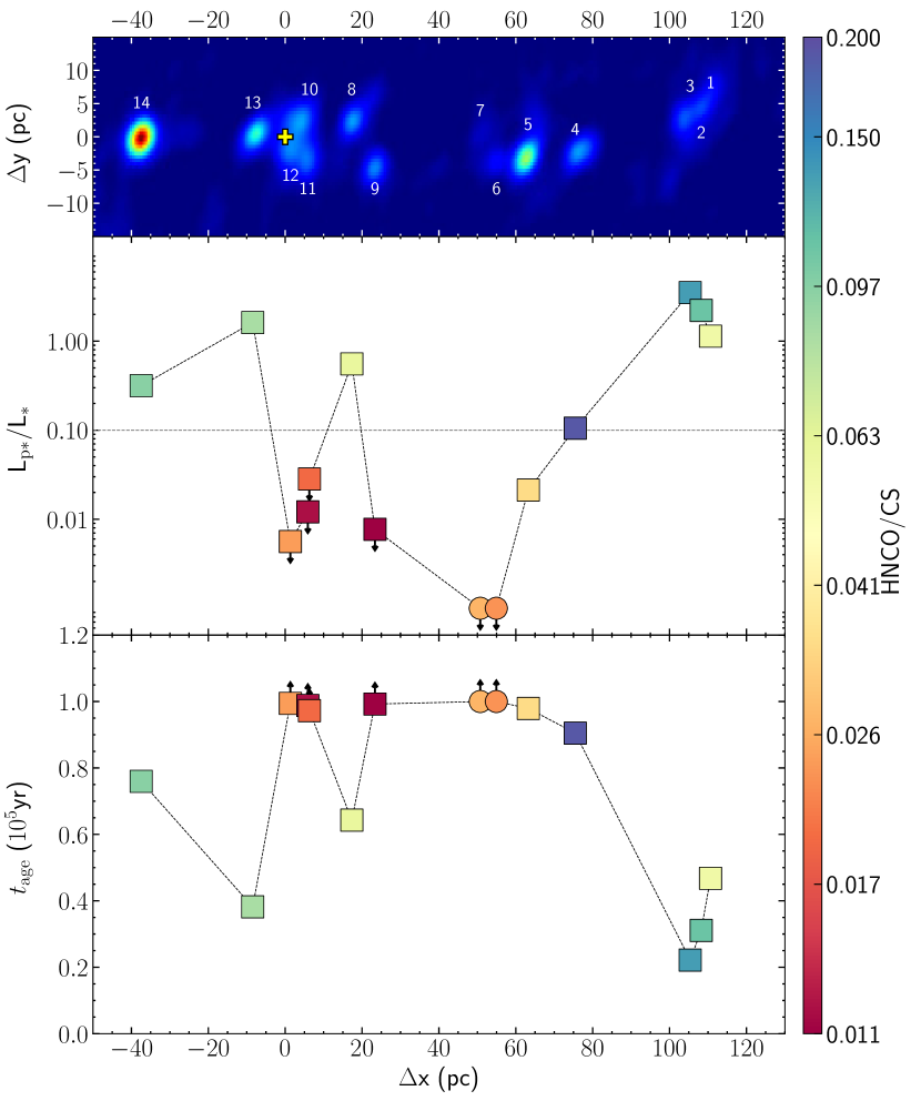
Figure 5: The top panel shows the rotated NGC 253 $218$ GHz continuum emission. TH2 is marked with a yellow cross. The middle panel shows proto and ZAMS stars luminosity ratio against the distance of each condensation to TH2. ZAMS-SSCs are indicated as upper limits. For sources $6$ and $7$, represented with circle, we have adopted a fiducial value of $\text{L}_{\text{p*}}/\text{L}_{*}=0.001$. The lower panel shows a rough estimation of the SSCs age based on its luminosity ratio $\text{L}_{\text{p*}}/\text{L}_{*}$ and assuming the timescale of an H ii region to be $10^{5}$ yr. Sources are colored by their HNCO/CS ratio.

The estimated age of the SSCs ($t_{\text{age}}$) in Fig. 5 shows a clear trend in their evolutionary stage as a function of their position. Central condensations in Fig. 5 ($4$, $5$, $6$, $7$, $9$, $10$, $11$ and $12$) are more evolved than the sources at the edges ($1$, $2$, $3$, $13$ and $14$). The exception of source $8$ could be explained if it were only apparently close to the center due to a projection effect.

6.1.2 Radiative feedback

Massive stars have a strong impact on their surroundings due to both mechanical and radiative feedback. Once the massive stars in the SSCs reach the UCHII region phase it is expected that the UV radiation will affect the surrounding material creating photodissociation regions (PDRs). Then one expects that the difference in the evolutionary stage found in the SSCs in NGC 253 will have an impact in the chemical richness of the molecular gas in SSCs. In fact, Ando et al. (2017) found that at scales of $10$ pc (at a lower resolution than in this work) the HNCO and CH₃OH abundances dramatically decreases in two of their sources, which actually contain our ZAMS-SSCs $10$, $11$, $12$ and $9$. Martín et al. (2008); Martín et al. (2009) have found that the HNCO/CS ratio is an excellent tracer of gas affected by UV radiation since HNCO is much more easily dissociated than CS (which is still abundant in PDRs). The rather low relative abundances of HNCO at scales of $10$ pc suggests that in ZAMS-SSCs the radiation from the newly formed O-type stars have already created PDRs, destroying a large fraction of molecular gas in their surroundings.

In order to better quantify the effect of the radiative feedback in the SSCs, we have derived from our data set the HNCO/CS ratio with the same angular resolution as the HC₃N data by using the integrated intensities of the HNCO $(16_{1,15}-15_{1,14})$ and CS $(7-6)$ lines towards all the SSCs, see Table 7. Panel a) of Figure 6 displays this ratio against the ratio between the stellar mass and the gas mass, $\text{M}_{*}/\text{M}_{\text{gas}}$. The HNCO/CS ratio is expected to be inversely related to the ratio of the number of UV photons (stellar mass) and the total gas mass.

Table 7: Observed integrated line emission in Jy beam^-1 km s^-1 for HNCO and CS lines.

HC	FWHM HNCO	HNCO	FWHM CS	CS
	$({}^{\text{km}}\!/_{\text{s}})$	$16_{1,15}-15_{1,14}$	$({}^{\text{km}}\!/_{\text{s}})$	$7-6$
$\nu$ (GHz)		352.90		342.88
$E_{LO}$ (K)		118.37		34.32
1	$17.0$	$0.117$	$42.0$	$2.09$
2	$33.2$	$0.275$	$49.6$	$2.53$
3	$23.0$	$0.272$	$57.3$	$2.03$
4	$27.8$	$0.226$	$36.2$	$1.44$
5	$44.0$	$0.267$	$41.4$	$7.81$
6	$38.0$	$\leqslant 0.046$	$38.0$	$1.01$
7	$40.0$	$\leqslant 0.043$	$39.6^{*}$	$0.88$
8	$24.5$	$0.160$	$37.0$	$2.66$
9	$33.2$	$\leqslant 0.060$	$37.6^{*}$	$2.08$
10	$34.8$	$0.055$	$35.5^{*}$	$2.84$
11	$50.8$	$0.065$	$56.4^{*}$	$5.45$
12	$40.0$	$0.082$	$55.8^{*}$	$3.37$
13	$32.0$	$0.293$	$46.0^{*}$	$3.48$
14	$45.0$	$1.463$	$42.0^{*}$	$15.19$

• ^∗ Two CS components or CS autoabsorption.

Figure 6a clearly shows two different regimes shown as blue ($\text{L}_{\text{p*}}/\text{L}_{*}$>0.1) and red ($\text{L}_{\text{p*}}/\text{L}_{*}$<0.1) shaded regions. The SSCs located in the red region, with large masses in stars as compared to their gas mass ($\text{M}_{*}/\text{M}_{\text{gas}}\gtrsim 1$), have already photo-dissociated most of their HNCO. Sources with HNCO/CS values $\lesssim 0.05$ ($12$, $11$, $10$, $9$, $7$, $6$ and $5$) are indeed the oldest and more evolved ones, with estimated ages around $\gtrsim 10^{5}$ yr. This result strongly suggests that radiative feedback has started to have an important effect in the chemical properties of the molecular gas left after star formation and it might have played a role in quenching the star formation on these sources. This is in agreement with their rather low $\text{L}_{\text{p*}}/\text{L}_{*}$ ratio of $<0.1$. On the other hand, the SSCs in the blue region with higher $\text{L}_{\text{p*}}/\text{L}_{*}$ and low $\text{M}_{*}/\text{M}_{\text{gas}}$ show rather high HNCO/CS, as expected if the UV radiation from the (few) recently formed stars do not significantly affect the chemical properties of the molecular gas due to the relatively low amount of stars in the ZAMS phase as compared to that in the protostar phase (high $\text{L}_{\text{p*}}/\text{L}_{*}$ ratios) or because it is very well shielded. This is expected for very young SSCs still forming stars, where the PDRs created by a still low fraction of massive stars in the ZAMS phase represents a small fraction of the total gas mass. Within this context, source $4$ would be in an intermediate state between these two phases, with high HNCO/CS ratio but rather low $\text{L}_{\text{p*}}/\text{L}_{*}$; and source $5$ would have reached the ZAMS phase recently. In summary, the overall chemical effects revealed by the HNCO/CS ratios suggest that it is consistent with the picture of the formation and evolution of SSCs, indicating that the radiative feedback effects appear relatively quick in just a few $10^{5}$  yr, when the SSCs seem to be completely formed.

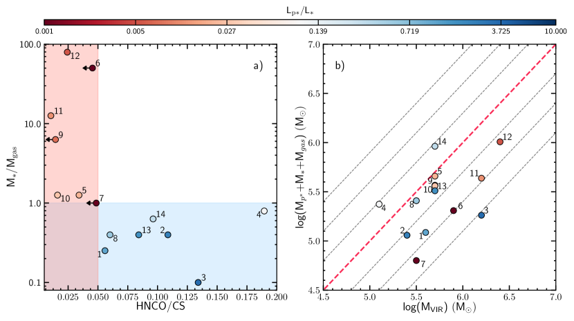
Figure 6: a) Radiative feedback: ratio between mass in form of stars and gas mass against the integrated intensity HNCO/CS ratio (i.e. radiative feedback). Blue and red shaded regions contains SSCs with $\text{L}_{\text{p*}}/\text{L}_{*}>0.1$ and $<0.1$, respectively. b) Mechanical feedback: virial mass from Leroy et al. (2018) against total mass (mass in gas, stars and protostars) for each SSC candidate. Sources are colored by their $\text{L}_{\text{p*}}/\text{L}_{*}$ ratio.

6.1.3 Mechanical Feedback

So far it is unclear whether the mechanical feedback produced by the massive stars in the proto and ZAMS phases plays a significant role in the very early stages of SSCs evolution. While radiation could permeate the whole SSC molecular cloud in very short timescales, depending on the number of ionizing stars and the extinction (i.e. the total dust column gas), the mechanical feedback is expected to have a longer time scale to have a sizeable effect on the whole cloud. This is due to the nature of mechanical feedback which is injected in the cloud by the winds of the proto and ZAMS stars in the SSCs. Usually, mechanical feedback is observed by means of P-Cygni profiles (González-Alfonso et al., 2012) or broad wings in the molecular line profiles. Alternatively, we can use the Virial Theorem to look how the total kinetic energy relates to the total potential energy of the SSCs. Leroy et al. (2018) have already discussed the dynamical mass and the stellar and gas content of the SSCs. We have updated the Leroy et al. (2018) Virial analysis by adding the protostar component found in this work to their stellar mass as shown in panel b) of Fig. 6. Some of the proto-SSCs are close to virialization ($5$, $8$, $13$), but most of them are not virialized. Although older ZAMS-SSCs seem to have a larger non-virialized state ($6$, $7$, $9$, $11$, $12$), as expected from mechanical feedback, also very young proto-SSCs (like $1$ and $3$) have larger dynamical masses than that in gas and stars. Hence, even taking into account the protostar component, the Virial analysis does not show any clear trend on the dynamical state of the SSCs related to mechanical feedback as one would expect from their evolution.

6.2 Star formation efficiency in the SSCs

The SFE of a molecular cloud with an initial mass $\text{M}_{\text{initial}}$ is given by the ratio between the mass converted into stars and the initial mass, ($\text{M}_{p*}+\text{M}_{*})/\text{M}_{\text{initial}}$. Assuming that there has not been significant mass loss, as inferred from the discussion above on the radiative and mechanical feedback, $\text{M}_{\text{initial}}$ can be estimated from the sum of the mass already in stars plus the remaining gas mass ($\text{M}_{p*}+\text{M}_{*}+\text{M}_{\text{gas}}$), will be given by

$$\frac{1}{1+\text{M}_{\text{gas}}/(\text{M}_{p*}+\text{M}_{*})}$$ (4)

In case that the mechanical feedback is not negligible, the derived SFEs must be considered as upper limits. Using this approach, we have estimated the SFEs shown in panel a) of Fig. 7 as a function of the age of the SSCs (derived from their L_p∗/L_∗ ratio), colored by their HNCO/CS ratio. It is remarkable that the SSCs show two different SFE regimes. The young proto-SSCs, including intermediate sources like $5$ and $10$ with SFEs of $\sim 30-60\%$ and the more evolved ZAMS-SSCs with SFEs $>85\%$. SSC $7$ is clearly outside this trend. It could be that it was not massive enough to maintain a high SFE, it has the lowest $\text{M}_{\text{initial}}=6.3\times 10^{4}$ M_⊙ while the other SSCs have $\text{M}_{\text{initial}}>1.2\times 10^{5}$ M_⊙.

The higher SFEs derived for the ZAMS-SSCs are in accordance with their evolutionary stage, since they are more evolved and have had more time to convert gas into stars. This is further supported by the correlation we have found (see Fig. 7b) between gas mass and age (i.e. L_p∗/L_∗) and also the radiative feedback (HNCO/CS ratio). In addition, if the proto-SSCs continue transforming gas into stars will finally also achieve a very high SFE of $>85\%$. A high SFE means that most of the stars have to be formed in a very short time scale because the feedback (radiative or mechanical) generated by the stars soon starts to halt the star formation. In addition, as discussed below, the “future” SFR should be high enough to complete the conversion of a large fraction of gas mass into stars (with the exception of source $7$).

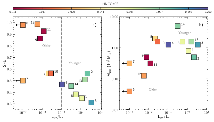
Figure 7: a) Star Formation Efficiency against luminosity ratio. b) SSC candidates gas mass versus their luminosity ratio. Sources are colored by their HNCO/CS ratio. The luminosity and the HNCO/CS ratios are used as proxies of the SSCs age.

6.3 Evolution of the star formation rates during the SSC formation

From the lifetimes and the stellar masses involved in the different phases of the formation of the SSCs, we can estimate the history of the SFRs during their formation. Let us first consider the SFRs required to form the stellar components in the proto and ZAMS star phases for all SSCs. Figure 8 shows the estimated SFRs for the stellar components as traced by the protostars ($\text{M}_{p*}/t_{\text{age}}$) and by the ZAMS stars ($\text{M}_{*}/t_{\text{age}}$), colored by their HNCO/CS ratio. The SFRs derived from ZAMS stars span from $\sim 0.5$ to $5.5$ M_⊙ yr^-1, not showing any systematic trend. For instance, SSCs $11$ and $14$, ZAMS and proto-SSCs respectively, show similar high ZAMS SFRs of $4$ and $5.5$ M_⊙ yr^-1. The SFRs derived for the protostars only applies to proto-SSCs, which are still forming stars and range from $\sim 2$ to $6$ M_⊙ yr^-1. The protostar SFRs of the ZAMS-SSCs is close to $0$. Most of the proto-SSCs ($1$, $2$, $3$, $13$) show somewhat higher protostar SFRs than ZAMS SFRs. However, sources $14$, $8$ and $4$ show just the opposite behaviour. However, given the uncertainties in our estimates we consider that the SFRs did not change between both phases. We can make a projection of the expected SFRs by considering that the final SFE of the proto-SSCs will be of about $0.95$, similar to that of the ZAMS-SSCs. It is noteworthy that basically all proto-SSCs require to maintain similar SFRs than those found in the previous phases to achieve a SFE of $\sim 0.95$. The only exception would be SSC $14$, which would require a very high SFR of $\sim 4$ M_⊙ yr^-1 to form the first massive stars already in the ZAMS phase; then decrease to $1$ M_⊙ yr^-1 for the newly formed stars (protostars in the SHCs); and finally would have to increase its SFR up to $10$ M_⊙ yr^-1 to archive a SFE of $\sim 0.95$ in $10^{5}$ yr.

The SFRs estimated for the different phases seem to be independent from the SSCs age or evolutionary phase. The SFRs of the SSCs ranges from $1$ to $4$ M_⊙ yr^-1, with the exception of SSCs $11$ and $14$, which show a SFR of $>4$ M_⊙ yr^-1. These are the only SSCs that show a SFR higher than the global value of $3-4$ M_⊙ yr^-1 (Ott et al., 2005; Bendo et al., 2015). While most of the proto-SSCs likely achieve SFEs of $\sim 1$, the evolution of the SSC $14$ is less clear since it will require a substantial increase in the SFR in the next few $10^{4}$ yr, however the radiative feedback is still negligible (high HNCO/CS ratio) and suggest that star formation could not be quenched in less than $10^{4}$ yr.

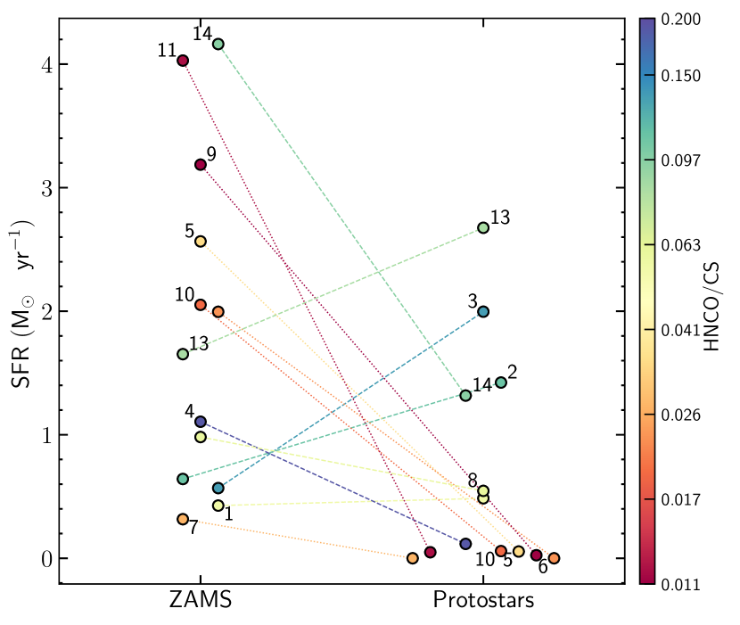
Figure 8: Derived SFRs for the different phases of SSCs. The ZAMS and protostars SFRs have been derived from the masses of the two stellar components and their estimated ages ($\text{M}_{*}/t_{\text{age}}$ and $\text{M}_{p*}/t_{\text{age}}$, respectively) .

6.4 On the evolution of SSCs in galaxies

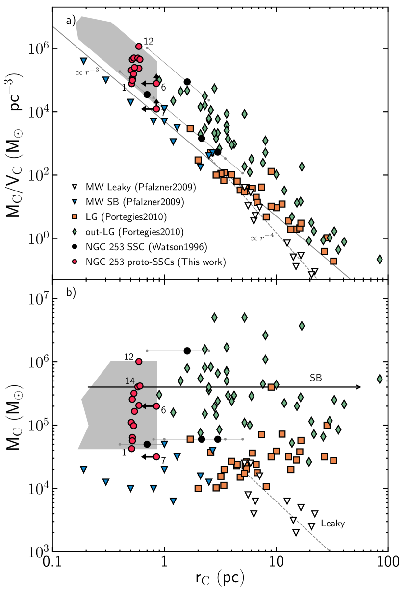
Figure 9: Comparison of the observed properties (densities, masses and radii) of the SSCs in NGC 253 with other SSCs. Red circles represent the SSCs in NGC 253 from this work. Their marker position is the mean between the upper and lower limit radii and the grey shadow their possible values from the lower to the upper size limit. Black circles are evolved SSCs in NGC 253 observed by Watson et al. (1996). Triangles are MW embedded clusters from Lada & Lada (2003). Colored and empty inverted triangles are MW SB and leaky clusters from Pfalzner (2009), respectively. Squares are SSCs from Local Group galaxies and diamonds are SSCs from outside the Local Group from Portegies Zwart et al. (2010). Panel a) shows the density-radius dependency, with the solid grey line indicating a $r^{-3}$ dependency for SB clusters (all colored symbols) and the dashed grey line a $r^{-4}$ dependency for the leaky clusters (inverted empty triangles). Panel b) shows the mass of these clusters against their radius.

So far, SSCs have only been observed in external galaxies (see Portegies Zwart et al., 2010, for a review) and they seem to be the only objects that can become a bound cluster as massive as GCs (Johnson et al., 2015). Pfalzner (2009, 2011) found that the most massive clusters in the MW evolve in two different sequences: clusters that sustain heavy mass losses expand faster (leaky or unbound clusters) than those that are able to overcome this losses (compact, bound or starburst clusters). Following Pfalzner (2009), in Fig. 9 we have plotted the cluster density ($\text{M}_{C}/\text{V}_{C}$) and the cluster mass ($\text{M}_{C}$), in panels a) and b) respectively, as a function of the cluster radius ($\text{r}_{C}$) (Lada & Lada, 2003; Pfalzner, 2009; Portegies Zwart et al., 2010, and references therein). The data include NGC 253 young SSCs from this paper (red circles, where $\text{M}_{C}=\text{M}_{p*}+\text{M}_{*}$) and Watson et al. (1996) evolved SSCs (black circles), SSCs in galaxies in the Local Group (LG, orange squares) and outside the LG (green diamonds) together. Also plotted are MW leaky (unbound) and starburst (SB, i.e. bound) clusters (inverted triangles Pfalzner, 2009). For the leaky clusters, the density evolves as $\propto r^{-4}$ (empty inverted triangles and dashed line in Fig. 9), while the density of SB clusters evolves as $\propto r^{-3}$ (blue inverted triangles and solid line in Fig. 9). This is also illustrated in the panel b) of Fig. 9 where we show how the cluster masses for SB clusters (colored symbols) remain more or less constant with their evolution but leaky clusters (empty symbols) masses changes as they evolve. The difference seems to be related to a higher SFE in SB clusters than in leaky clusters. Pfalzner & Kaczmarek (2013) studied the SFEs required for clusters given a certain density and radius, finding that leaky clusters with SFEs $\sim 20\%$ would not be able to be identified as overdensities after $>5-10$ Myr as with this SFE the cluster density declines rapidly. For SB clusters, Pfalzner & Kaczmarek (2013) find higher SFEs ($\sim 60-70\%$), but higher SFEs ($\geqslant 80\%$) would not explain the observed sizes $>1$ pc for $>10$ Myr old clusters. Panel a) of Fig. 9 shows that young SSCs in NGC 253 lay in the upper part of the evolutionary sequence of SSCs, i.e. small sizes ($r\lesssim 0.85$ pc) and high densities ($\sim 10^{5}-10^{6}$ M_⊙ pc^-3), as expected from young SSCs still unaffected by mechanical feedback. If the SFE is one of the key parameters that determines the survival of a cluster as a bounded system, the high SFEs ($\gtrsim 50\%$) derived for the SSCs detected in NGC 253 suggests that they could evolve into GCs. But what mechanisms favour such a high SFE is so far unknown. However, external pressure has to be high enough and it has been proposed to be one of the mechanisms that can maintain high SFRs over enough time to achieve such high SFEs (Keto et al., 2005; Beck, 2015; Johnson et al., 2015, and references therein).

6.5 On the formation of SSCs

The physical processes leading to massive star formation from the natal molecular cloud are still not well understood (see Zinnecker & Yorke, 2007, for a review). In fact, the formation and early evolution of the extreme SSCs found in galaxies is one of the most important challenges in the field of star formation. Several competing theories have been proposed to form massive stars: i) Monolithic core accretion (McKee & Tan, 2002, 2003); ii) Competitive accretion (proposed by Bonnell et al., 2001). In the monolithic core accretion, different mechanisms (radiative feedback, gas turbulence and magnetic fields) prevent high fragmentation of the molecular cloud. Then, the densest parts of the cloud have enough material in their surroundings to allow the formation of, at most, a few massive stars. In contrast, in the competitive accretion scenario the cloud fragments and first form a cluster of low-mass stars increasing the cloud gravitational potential well. This helps to accrete the remaining surrounding gas, which is funneled by the low-mass star cluster leading to clustered high-mass stars in the cloud center. Observational evidences supporting the competitive accretion scenario have been found in several massive star-forming regions (e.g. Rivilla et al., 2013b, a, 2014). In a very high density low-mass star cluster, the coalescence of two or more stars might be able to form a more massive star (Bonnell et al., 2001). Monolithic core accretion has to face the problem of preventing the further fragmentation of a core in order to be able to form massive stars (Hennebelle & Commerçon, 2014) making very unlikely the formation of SSCs with high SFEs in very short timescales. On the other hand, Competitive accretion successfully reproduces the observed stellar Initial Mass Function (IMF) of most MW stellar clusters. Yet, in order to form SSCs like the ones observed in NGC 253, the phase of the initial low-mass star cluster accretion has to be long enough to accrete enough gas, with large mass accretion rates, to form a SSC (M${}_{*}\gtrsim 10^{5}$ M_⊙). Like for the monolithic collapse, the extremely high SFEs and the very short timescales for the SSC formation poses very strong constrains on the timescales for the cluster formation once all the mass has been accreted in a relatively long time scale. This is even more severe for the formation of massive stars by the coalescence of low-mass stars.

The trend found in the SSCs estimated age ($t_{\text{age}}$), with the more evolved SSCs at smaller projected distances from the galaxy center (see Fig. 5), provides an indication of the recent history of the SSC formation within the inner $160$ pc of NGC 253. The obvious explanation would be that the formation of the SSCs is propagating from the center of the galaxy outwards.

Figure 10 shows, together with the young SSCs studied in this work, the location of the Super Nova Remnants (SNR) and H ii regions observed by Ulvestad & Antonucci (1997) between $1.3-20$ cm with the VLA; the stellar clusters observed in the IR by Fernández-Ontiveros et al. (2009); the more evolved SSCs observed by Watson et al. (1996) with the HST (ages of $5-100\times 10^{6}$ yr); and the positions of two X-ray sources as seen by Chandra (Müller-Sánchez et al., 2010), along with the position of the brightest radio source TH2 (Turner & Ho, 1985) and the kinematical center proposed by Müller-Sánchez et al. (2010). While most of the H ii regions are associated to the young SSCs discussed, the SNRs and the old SSCs are located below and above the projected ridge of young SSCs, being plausible that some of the old SSCs and SNRs are located in the spiral arms.

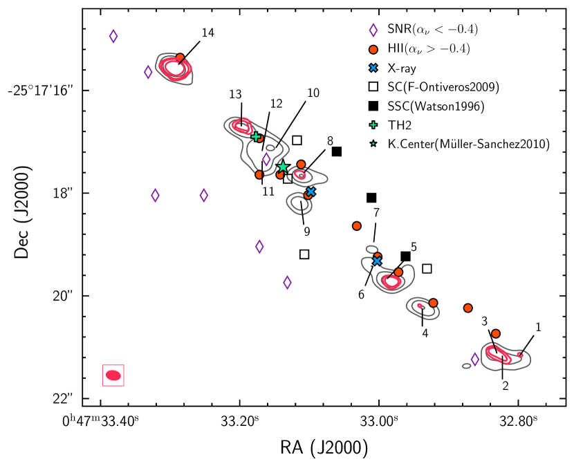
Figure 10: NGC 253 nuclear region. On grey and red contours are plotted the $218$ GHz continuum and the HC₃N $v_{7}=1$ $24-23$ emission, respectively. The numbers indicate the position of the forming SSCs discussed in this work. Also indicated are the positions of SNRs with open puple diamonds and H ii regions with orange circles, studied by Ulvestad & Antonucci (1997). Open squares show the position of stellar clusters (SCs) observed by Fernández-Ontiveros et al. (2009) and filled squares the SSCs observed by Watson et al. (1996). The blue crosses indicate the positions of X-1 and X-2 (coincident with the radio source TH7) (Müller-Sánchez et al., 2010). The position of TH2 (Turner & Ho, 1985) and the kinematical center (from Müller-Sánchez et al., 2010) are indicated by a teal plus and star symbol, respectively. The latter has a $3\sigma\sim 1.2^{\prime\prime}$ uncertainty in its position.

The main properties observed and derived in this work for the SSCs in NGC 253 (youth, massive, high SFEs and relatively constant SFRs) favours the idea that SSC formation in galaxies represent the most extreme mode of star formation and that it seems to be triggered by external events. Events like galaxy merging, density waves, and mechanical feedback from an active nucleus and/or from star formation will lead to strong shocks which will heat and compress the gas to the sizes and densities required to form the SSCs. In the case of the SSCs observed in NGC 253, the most likely explanation would be the overpressure produced by hot gas generated by the SN explosion(s) from an early star formation episode in the galaxy center. The trend observed in the age of the SSCs as a function of their location indicates that this might have been produced by a single event.

7 Conclusions

We have used ALMA to study the earliest phases of the formation and evolution of Super Star Clusters (SSCs) which are still deeply embedded in their parental molecular cloud. By using $0.2^{\prime\prime}$ resolution ($\sim 3$ pc) ALMA images of the HC₃N vibrational excited emission (HC₃N^∗) we have revealed the Super Hot Core (SHC) phase associated with young SSCs (proto-SSCs) in the inner ($160$ pc) region of the nucleus of the nearby starburst galaxy NGC 253. Our main results can be summarized as follows:

1.

From the $14$ forming SSCs with strong free-free and dust emission, we have found that $8$ of them show HC₃N^∗ emission (SHC phase), another $4$ show only HC₃N emission from the ground state and $2$ of them do not show HC₃N emission.

2.

We have carried LTE and non-LTE modelling of the HC₃N^∗ emission to derive the main properties of the SHCs, finding high dust temperatures of $200-375$ K and relatively high H₂ densities of $1-6\times 10^{6}$ cm^-3. Somewhat lower temperatures ($\sim 130$ K) but similar densities are found for the remaining sources with no HC₃N^∗ emission. We have also estimated, from the lower limit to their sizes, that the LTE and non-LTE IR luminosities of the SHCs range from $0.1$ to $1\times 10^{8}$ L_⊙.

3.

The SHCs represent a short lived (a few $10^{4}$ yr) phase in the formation of massive stellar clusters, just when protostars are still accreting mass right before massive stars reach the Zero Age Main Sequence (ZAMS) and ionize their surroundings creating Ultra Compact H ii (UCHII) regions. We have estimated the total stellar mass content of the SSCs in ZAMS stars (M_∗), from free-free emission inside UCHII regions (Leroy et al., 2018), and in protostars (M_p∗), from the IR luminosities. The derived total masses range from $0.6$ to $10\times 10^{5}$ M_⊙. However, the proto/ZAMS luminosity ratio ($\text{L}_{p*}/\text{L}_{*}$) in the SSCs shows large variations, of more than two orders of magnitude, from $3.5$ to $<0.01$, indicating that the SSCs are in different evolutionary stages.

4.

We have then used the $\text{L}_{p*}/\text{L}_{*}$ ratio as a clock to measure the evolutionary stage ($t_{\text{age}}$) of the SSCs. We estimate that the ages of the youngest SSCs, showing the largest luminosity ratios ($>0.1$), must be a few $10^{4}$ yr, and are dominated by the protostar phase (i.e proto-SSCs). The older ones, with lower luminosity ratios are dominated by the ZAMS phase, are considered ZAMS-SSCs and are likely to be less than $10^{6}$ yr since we do not find evidence of mechanical feedback.

5.

The evolutionary scenario presented above is also supported by the radiative feedback as traced by the HNCO/CS ratio, which measures the degree of photodissociaton of the bulk of the molecular gas in the SSCs. This ratio is systematically higher in the young proto-SSC than in the older ones, as expected if the strong UV radiation from the OB stars in the ZAMS-SSCs has permeated the whole SSC.

6.

The estimated Star Formation Efficiency (SFE), obtained assuming there has not been significant mass loss (supported by the previous mechanical and radiative feedback analysis) increases from $\sim 40\%$ for the proto-SSCs to $>85\%$ for the ZAMS-SSCs. Yet, the gas mass reservoir available for star formation in the proto-SSCs ($1-7\times 10^{5}$ M_⊙) is much larger, by nearly one order of magnitude, than in the ZAMS-SSCs ($0.3-7\times 10^{4}$ M_⊙), supporting the scenario that star formation is still going on inside the proto-SSCs.

7.

The SFRs derived for the ZAMS and proto-SSCs phases have similar values, covering a wide range from $0.5$ to $4$ M_⊙ yr^-1. For all proto-SSCs we find that the SFR required to achieve a final SFE similar to those of the ZAMS-SSCs ($\sim 95\%$) remains constant during their evolution within a factor of $2$.

8.

We find a systematic trend between the estimated age of the SSCs and their projected location in the nuclear region, with the older ZAMS-SSCs located around the center of the galaxy and the younger proto-SSCs in the outer regions, suggesting an inside-out SSCs formation scenario. We consider that the formation and the high SFE of the SSCs were very likely triggered by the overpressure due to external event(s) that propagates from the inner to the outer nuclear regions.

References

- Alonso-Herrero et al. (2003) Alonso-Herrero A., Rieke G. H., Rieke M. J., Scoville N. Z., 2003, in Perez E., Gonzalez Delgado R. M., Tenorio-Tagle G., eds, Astronomical Society of the Pacific Conference Series Vol. 297, Star Formation Through Time. p. 197 (arXiv:astro-ph/0211485)
- Ando et al. (2017) Ando R., et al., 2017, ApJ, 849, 81
- Astropy Collaboration et al. (2013) Astropy Collaboration et al., 2013, A&A, 558, A33
- Báez-Rubio et al. (2014) Báez-Rubio A., Martín-Pintado J., Thum C., Planesas P., Torres-Redondo J., 2014, A&A, 571, L4
- Báez-Rubio et al. (2018) Báez-Rubio A., Martín-Pintado J., Rico-Villas F., Jiménez-Serra I., 2018, ApJ, 867, L6
- Barcos-Muñoz et al. (2015) Barcos-Muñoz L., et al., 2015, ApJ, 799, 10
- Beck (2015) Beck S., 2015, International Journal of Modern Physics D, 24, 1530002
- Bendo et al. (2015) Bendo G. J., Beswick R. J., D’Cruze M. J., Dickinson C., Fuller G. A., Muxlow T. W. B., 2015, MNRAS, 450, L80
- Bonnell et al. (2001) Bonnell I. A., Bate M. R., Clarke C. J., Pringle J. E., 2001, MNRAS, 323, 785
- Churchwell (2002) Churchwell E., 2002, ARA&A, 40, 27
- Clark et al. (2005) Clark J. S., Negueruela I., Crowther P. A., Goodwin S. P., 2005, A&A, 434, 949
- Costagliola & Aalto (2010) Costagliola F., Aalto S., 2010, A&A, 515, A71
- De Pree et al. (2014) De Pree C. G., et al., 2014, ApJ, 781, L36
- DeLeon & Muenter (1985) DeLeon R. L., Muenter J. S., 1985, The Journal of chemical physics, 82, 1702
- Deguchi et al. (1979) Deguchi S., Nakada Y., Onaka T., Uyemura M., 1979, PASJ, 31, 105
- Donnison & Williams (1976) Donnison J. R., Williams I. P., 1976, Nature, 261, 674
- Doran et al. (2013) Doran E. I., et al., 2013, A&A, 558, A134
- Faure et al. (2016) Faure A., Lique F., Wiesenfeld L., 2016, MNRAS, 460, 2103
- Fernández-Ontiveros et al. (2009) Fernández-Ontiveros J. A., Prieto M. A., Acosta-Pulido J. A., 2009, MNRAS, 392, L16
- Garay & Lizano (1999) Garay G., Lizano S., 1999, PASP, 111, 1049
- Goldsmith et al. (1982) Goldsmith P. F., Snell R. L., Deguchi S., Krotkov R., Linke R. A., 1982, ApJ, 260, 147
- Goldsmith et al. (1983) Goldsmith P. F., Krotkov R., Snell R. L., Brown R. D., Godfrey P., 1983, ApJ, 274, 184
- González-Alfonso & Cernicharo (1997) González-Alfonso E., Cernicharo J., 1997, A&A, 322, 938
- González-Alfonso & Cernicharo (1999) González-Alfonso E., Cernicharo J., 1999, ApJ, 525, 845
- González-Alfonso & Sakamoto (2019) González-Alfonso E., Sakamoto K., 2019, arXiv e-prints, p. arXiv:1908.04058
- González-Alfonso et al. (2012) González-Alfonso E., et al., 2012, A&A, 541, A4
- González-Alfonso et al. (2014) González-Alfonso E., Fischer J., Aalto S., Falstad N., 2014, A&A, 567, A91
- González-Alfonso et al. (2015) González-Alfonso E., et al., 2015, ApJ, 800, 69
- Hennebelle & Commerçon (2014) Hennebelle P., Commerçon B., 2014, in Stamatellos D., Goodwin S., Ward-Thompson D., eds, Astrophysics and Space Science Proceedings Vol. 36, The Labyrinth of Star Formation. p. 365, doi:10.1007/978-3-319-03041-8_72
- Hills (1980) Hills J. G., 1980, ApJ, 235, 986
- Hoare et al. (2007) Hoare M. G., Kurtz S. E., Lizano S., Keto E., Hofner P., 2007, Protostars and Planets V, pp 181–196
- Hosokawa & Omukai (2009) Hosokawa T., Omukai K., 2009, ApJ, 691, 823
- Ivezic & Elitzur (1997) Ivezic Z., Elitzur M., 1997, MNRAS, 287, 799
- Jaffe & Martín-Pintado (1999) Jaffe D. T., Martín-Pintado J., 1999, ApJ, 520, 162
- Johnson et al. (2015) Johnson K. E., Leroy A. K., Indebetouw R., Brogan C. L., Whitmore B. C., Hibbard J., Sheth K., Evans A. S., 2015, ApJ, 806, 35
- Keto et al. (2005) Keto E., Ho L. C., Lo K. Y., 2005, ApJ, 635, 1062
- Kornei & McCrady (2009) Kornei K. A., McCrady N., 2009, ApJ, 697, 1180
- Kurtz et al. (2000) Kurtz S., Cesaroni R., Churchwell E., Hofner P., Walmsley C. M., 2000, Protostars and Planets IV, pp 299–326
- Lada & Lada (2003) Lada C. J., Lada E. A., 2003, ARA&A, 41, 57
- Larson & Tinsley (1978) Larson R. B., Tinsley B. M., 1978, ApJ, 219, 46
- Leroy et al. (2018) Leroy A. K., et al., 2018, ApJ, 869, 126
- Martín-Pintado et al. (2005) Martín-Pintado J., Jiménez-Serra I., Rodríguez-Franco A., Martín S., Thum C., 2005, ApJ, 628, L61
- Martín et al. (2008) Martín S., Requena-Torres M. A., Martín-Pintado J., Mauersberger R., 2008, ApJ, 678, 245
- Martín et al. (2009) Martín S., Martín-Pintado J., Mauersberger R., 2009, ApJ, 694, 610
- Martín et al. (2011) Martín S., et al., 2011, A&A, 527, A36
- Martín et al. (2016) Martín S., et al., 2016, A&A, 590, A25
- Martín et al. (2019) Martín S., Martín-Pintado J., Blanco-Sánchez C., Rivilla V. M., Rodríguez-Franco A., Rico-Villas F., 2019, arXiv e-prints, p. arXiv:1909.02147
- McKee & Tan (2002) McKee C. F., Tan J. C., 2002, Nature, 416, 59
- McKee & Tan (2003) McKee C. F., Tan J. C., 2003, ApJ, 585, 850
- McMullin et al. (2007) McMullin J. P., Waters B., Schiebel D., Young W., Golap K., 2007, in Shaw R. A., Hill F., Bell D. J., eds, Astronomical Society of the Pacific Conference Series Vol. 376, Astronomical Data Analysis Software and Systems XVI. p. 127
- Melo et al. (2002) Melo V. P., Pérez García A. M., Acosta-Pulido J. A., Muñoz-Tuñón C., Rodríguez Espinosa J. M., 2002, ApJ, 574, 709
- Müller-Sánchez et al. (2010) Müller-Sánchez F., González-Martín O., Fernández-Ontiveros J. A., Acosta-Pulido J. A., Prieto M. A., 2010, ApJ, 716, 1166
- Müller et al. (2001) Müller H. S. P., Thorwirth S., Roth D. A., Winnewisser G., 2001, A&A, 370, L49
- Müller et al. (2005) Müller H. S. P., Schlöder F., Stutzki J., Winnewisser G., 2005, Journal of Molecular Structure, 742, 215
- Osorio et al. (1999) Osorio M., Lizano S., D’Alessio P., 1999, ApJ, 525, 808
- Ott et al. (2005) Ott J., Weiss A., Henkel C., Walter F., 2005, ApJ, 629, 767
- Pfalzner (2009) Pfalzner S., 2009, A&A, 498, L37
- Pfalzner (2011) Pfalzner S., 2011, A&A, 536, A90
- Pfalzner & Kaczmarek (2013) Pfalzner S., Kaczmarek T., 2013, A&A, 559, A38
- Pickett et al. (1998) Pickett H. M., Poynter R. L., Cohen E. A., Delitsky M. L., Pearson J. C., Müller H. S. P., 1998, J. Quant. Spectrosc. Radiative Transfer, 60, 883
- Portegies Zwart et al. (2010) Portegies Zwart S. F., McMillan S. L. W., Gieles M., 2010, ARA&A, 48, 431
- Rekola et al. (2005) Rekola R., Richer M. G., McCall M. L., Valtonen M. J., Kotilainen J. K., Flynn C., 2005, MNRAS, 361, 330
- Rivilla et al. (2013a) Rivilla V. M., Martín-Pintado J., Sanz-Forcada J., Jiménez-Serra I., Rodríguez-Franco A., 2013a, MNRAS, 434, 2313
- Rivilla et al. (2013b) Rivilla V. M., Martín-Pintado J., Jiménez-Serra I., Rodríguez-Franco A., 2013b, A&A, 554, A48
- Rivilla et al. (2014) Rivilla V. M., Jiménez-Serra I., Martín-Pintado J., Sanz-Forcada J., 2014, MNRAS, 437, 1561
- Rivilla et al. (2017) Rivilla V. M., Beltrán M. T., Cesaroni R., Fontani F., Codella C., Zhang Q., 2017, A&A, 598, A59
- Shimonishi et al. (2016) Shimonishi T., Onaka T., Kawamura A., Aikawa Y., 2016, The Astrophysical Journal, 827, 72
- Turner & Ho (1985) Turner J. L., Ho P. T. P., 1985, ApJ, 299, L77
- Ulvestad & Antonucci (1997) Ulvestad J. S., Antonucci R. R. J., 1997, ApJ, 488, 621
- Uyemura et al. (1982) Uyemura M., Deguchi S., Nakada Y., Onaka T., 1982, Bulletin of The Chemical Society of Japan - BULL CHEM SOC JPN, 55, 384
- Walmsley (1995) Walmsley M., 1995, in Lizano S., Torrelles J. M., eds, Revista Mexicana de Astronomia y Astrofisica Conference Series Vol. 1, Revista Mexicana de Astronomia y Astrofisica Conference Series. p. 137
- Watson et al. (1996) Watson A. M., et al., 1996, AJ, 112, 534
- Whitmore (2002) Whitmore B. C., 2002, in Geisler D. P., Grebel E. K., Minniti D., eds, IAU Symposium Vol. 207, Extragalactic Star Clusters. p. 367
- Whitmore & Schweizer (1995) Whitmore B. C., Schweizer F., 1995, AJ, 109, 960
- Wood & Churchwell (1989) Wood D. O. S., Churchwell E., 1989, ApJS, 69, 831
- Wyrowski et al. (1999) Wyrowski F., Schilke P., Walmsley C. M., 1999, A&A, 341, 882
- Zinnecker & Yorke (2007) Zinnecker H., Yorke H. W., 2007, ARA&A, 45, 481
- de Vicente et al. (2000) de Vicente P., Martín-Pintado J., Neri R., Colom P., 2000, A&A, 361, 1058
- de Vicente et al. (2002) de Vicente P., Martín-Pintado J., Neri R., Rodríguez-Franco A., 2002, ApJ, 574, L163