Fractional skyrmion and absence of low-lying Andreev bound states in a micro fractional-flux quantum vortex

Abstract

We investigate quasi-particle excitation modes and the topological number of a fractional-flux quantum vortex in a layered (multi-component) superconductor. The Bogoliubov equation for a half-flux quantum vortex is solved to show that there is no low-lying Andreev bound state near zero energy in the core of a quantum vortex, which is surprisingly in contrast to the result for an inter-flux vortex. Related to this result, there are singular excitation modes that have opposite angular momenta, moving in the opposite direction around the core of the vortex. The topological index (skyrmion number) for a fractional-flux quantum vortex becomes fractional since the topological index is divided into two parts where one from the vortex (bulk) and the other from the kink (domain wall, boundary). The topological numbers for both the vortex and the kink (domain wall) are fractional, and their sum becomes an integer. This shows an interesting analogy between this result and the index theorem for manifolds with boundary. We argue that fractional-flux quantum vortices are not commutative each other and follow non-abelian statistics. This non-abelian statistics of vortices is different from that in p-wave superconductors.

1 Introduction

Multi-component superconductivity has been studied intensively[1, 2, 3, 4, 5, 6, 7, 8, 9, 10, 11, 12, 13, 14]. There appear many significant phenomena in multi-component superconductors such as time-reversal symmetry breaking[5, 6, 7, 8, 9, 10, 11, 12, 13, 14, 15, 16], the appearance of massless modes[17, 18, 19, 20, 21, 22, 23, 24], the existence of fractional-flux quantum vortices[9, 25, 26, 27, 28, 29, 30, 31, 32, 33, 34, 35, 36, 37, 38, 39, 40], and unconventional isotope effect[41, 42, 43]. A fractional-flux quantum vortex (FFQV) has been examined in the study of multi-component superconductors. The existence of an FFQV has been proposed theoretically in multi-component superconductors and there have been several experimental attempts to observe FFQVs. Recently, the observation of an FFQV in an Nb thin film superconducting (SC) bilayer has been reported as a magnetic flux distribution image by using a scanning superconducting quantum interference device (SQUID) microscope[38]. It is then important to clarify quasi-particle excitation modes in an FFQV and a half-flux quantum vortex (HFQV) in multi-component or layered superconductors.

An FFQV has the fractional vorticity $Q$ where the magnetic flux in an FFQV is $Q\phi_{0}$ for the unit quantum flux $\phi_{0}=h/2|e|$ (in MKS units). An FFQV can be regarded as a micro vortex ($Q<1$) which is defined against the giant vortex[44]. We have $Q=1/2$ for an HFQV. The existence of a fractional-flux quantum vortex is strongly related to the existence of a kink solution in the phase space of SC gaps. In a two-gap superconductor, we have two global phases $\phi_{1}$ and $\phi_{2}$ associated with two SC gaps. The phase difference, defined by $\varphi=\phi_{1}-\phi_{2}$, satisfies the sine-Gordon equation, $\partial^{2}\varphi/\partial y^{2}-\alpha\sin\varphi=0$, where $\alpha$ is a constant and we assume that $\varphi$ has spatial dependence in the direction $y$. Since the cosine potential is a function of period $2\pi$, there is a kink solution satisfying the boundary condition that $\varphi\rightarrow 0$ as $y\rightarrow-\infty$ and $\varphi\rightarrow 2\pi$ as $y\rightarrow\infty$. An HFQV exists at the end of the kink[9, 45]. This is because a net-change of $\phi_{1}$ is $2\pi$ by a counterclockwise encirclement of the vortex and that of $\phi_{2}$ vanishes by including contributions from the kink. We can define the total vorticity $Q_{T}$ as the net-change of phase $\phi_{i}$ divided by $2\pi$. We have $Q_{T}=1$ for one band and $Q_{T}=0$ for the other band.

In this paper, we investigate the quasi-particle excitation modes in an FFQV. The Bogoliubov equation for an HFQV is solved numerically to obtain the energy spectra of excitation modes. We show that there are no quantized excitation modes near zero energy in the core of an HFQV, indicating the absence of low-lying Andreev bound states. There are quantized excitation modes in the kink as well, which are Andreev bound states since the gap function changes its sign when going across the kink. We also show that the topological number $N_{vortex}$, which is just regarded as the skyrmion number, becomes fractional for an FFQV: $N_{vortex}=Q$. The kink also has the fractional topological number. This is a phenomenon that the part of the index number is absorbed into the boundary (kink). Lastly, we argue that two half-flux quantum vortices are not commutative, namely, they follow non-abelian statistics.

2 Bogoliubov Equation for an FFQV

The SC gap function is written as

$$\Delta({\bf r})=\Delta_{0}(r)\exp(-iQ\phi),$$ (1)

where $\Delta_{0}(r)=\Delta_{\infty}\tanh(r/\xi_{0})$ for $r=|{\bf r}|$ and $Q$ is the vorticity. $\xi_{0}$ is the coherence length defined by $\xi_{0}=\hbar v_{F}/\Delta_{\infty}$ with the Fermi velocity $v_{F}$. $\phi=\phi(\theta)$ is a function of the angle variable $\theta$. In the absence of a kink, we have $\phi(\theta)=\theta$ for all $\theta$. For an HFQV ($Q=1/2$) in a two-component (bilayer) superconductor, there is the kink where the phase $\phi$ changes abruptly. The behaviors of $\phi_{i}(\theta)$ ($i=1,2$) for two gaps as a function of $\theta$ are shown in Fig. 1 and Fig. 2 for the first band and second band, respectively. In these figures, $\phi_{1}$ and $\phi_{2}$ are shown as a step function for simplicity, which we call the step function approximation. We show the phase $\phi_{2}$ as a function of two-dimensional coordinates $x$ and $y$ in Fig. 3. In this paper we consider only one band (one layer) by assuming that the Josephson coupling is small. The Bogoliubov equation for an FFQV reads

$$\left(\begin{array}[]{cc}-\frac{\hbar^{2}}{2m}{\bf\nabla}^{2}-\epsilon_{F}&\Delta({\bf r})\\ \Delta^{*}({\bf r})&\frac{\hbar^{2}}{2m}{\bf\nabla}^{2}+\epsilon_{F}\\ \end{array}\right)\left(\begin{array}[]{c}u_{j}({\bf r})\\ v_{j}({\bf r})\\ \end{array}\right)=\varepsilon_{j}\left(\begin{array}[]{c}u_{j}({\bf r})\\ v_{j}({\bf r})\\ \end{array}\right),$$ (8)

where $j$ refers to a quantum number representing a quantum level and $\epsilon_{F}$ indicates the Fermi energy. We have neglected the vector potential by assuming the high Ginzburg-Landau parameter. We write the wave function in the form,

$$\Psi_{j}({\bf r}) \equiv \left(\begin{array}[]{c}u_{j}({\bf r})\\ v_{j}({\bf r})\\ \end{array}\right)=e^{-iQ\sigma_{3}\phi/2}e^{i\mu\phi}\left(\begin{array}[]{c}\tilde{u}_{\mu n}({\bf r})\\ \tilde{v}_{\mu n}({\bf r})\\ \end{array}\right)$$ (14)

$$= \left(\begin{array}[]{c}e^{i(\mu-Q/2)\phi}\tilde{u}_{\mu n}({\bf r})\\ e^{i(\mu+Q/2)\phi}\tilde{v}_{\mu n}({\bf r})\\ \end{array}\right),$$ (17)

where $\sigma_{3}$ is the Pauli matrix. $n$ ia a radial quantum number and $\mu$ denotes the angular momentum written as $L_{z}=\mu\hbar$. We use the same parametrization as for a giant vortex[44]. In the absence of a kink, $\tilde{u}_{\mu n}$ and $\tilde{v}_{\mu n}$ depend only the radial variable $r$.

The Bogoliubov equation for particle and hole like excitations is

$$\sigma_{3}\frac{\hbar^{2}}{2m}\Bigg{[}-\frac{\partial^{2}f}{\partial r^{2}}-\frac{1}{r}\frac{\partial f}{\partial r}-\frac{1}{r^{2}}\frac{\partial^{2}f}{\partial\theta^{2}}-k_{F}^{2}f$$

$$+\left(\mu-\frac{Q}{2}\sigma_{3}\right)^{2}\frac{1}{r^{2}}\left(\frac{\partial\phi}{\partial\theta}\right)^{2}f-i\left(\mu-\frac{Q}{2}\sigma_{3}\right)\frac{1}{r^{2}}\frac{\partial^{2}\phi}{\partial\theta^{2}}f$$

$$-2i\left(\mu-\frac{Q}{2}\sigma_{3}\right)\frac{1}{r^{2}}\frac{\partial\phi}{\partial\theta}\frac{\partial f}{\partial\theta}\Bigg{]}+\sigma_{1}\Delta_{0}(r)f=\epsilon_{\mu n}f,$$ (18)

where we put

$$f=f({\bf r})=f(r,\theta)=\left(\begin{array}[]{c}\tilde{u}_{\mu n}({\bf r})\\ \tilde{v}_{\mu n}({\bf r})\\ \end{array}\right).$$ (21)

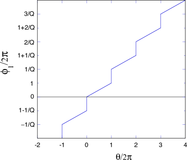
Figure 1: (Color online) Phase $\phi_{1}$ of the first band as a function of the angle variable $\theta$ within the step-function approximation. $\phi_{1}$ changes at $\theta=2\pi n$ for integer $n$. $Q$ is the vorticity of a vortex and the phase of the first gap is given by $Q\phi_{1}$. The scale of vertical axis corresponds to $Q=1/2$.

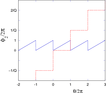
Figure 2: (Color online) Phase $\phi_{2}$ of the second band as a function of the angle variable $\theta$ within the step-function approximation. The dashed line indicates the phase difference $\phi_{1}-\phi_{2}$. $\phi_{2}$ changes at $\theta=2\pi k$ for integer $k$. $Q$ is the vorticity of a vortex. The scale of vertical axis corresponds to $Q=1/2$.

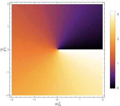
Figure 3: (Color online) Phase $Q\phi_{2}=\phi_{2}/2$ for $Q=1/2$ in the second layer as a function of two-dimensional coordinates $x$ and $y$. There is a kink on the positive part of $x$ axis.

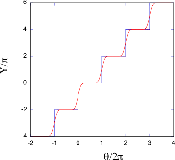
Figure 4: (Color online) $Y(\theta)$ as a function of $\theta$ for $Q=1/2$. $Y(\theta)$ is given by a step function in the step-function approximation for the kink. In general, $Y(\theta)$ is a smooth function of $\theta$ as shown by the curve in the figure.

3 Wave Function of Variable Separation Form

We will find a solution of the variable separation form:

$$f(r,\theta)=\exp\left(iY(\theta)\hat{C}\right)g(r),$$ (22)

where $\hat{C}$ is a constant matrix, $Y(\theta)$ is a function of $\theta$ and $g(r)$ is a radial function of $r=|{\bf r}|$. The equation for $g(r)$ and $Y(\theta)$ reads

$$\sigma_{3}\frac{\hbar^{2}}{2m}\Big{[}-\frac{\partial^{2}g}{\partial r^{2}}-\frac{1}{r}\frac{\partial g}{\partial r}-\left(iY^{\prime\prime}(\theta)\hat{C}-Y^{\prime}(\theta)^{2}K^{2}\right)\frac{1}{r^{2}}g-k_{F}^{2}g$$

$$+\left(\mu-\frac{Q}{2}\sigma_{3}\right)^{2}\frac{1}{r^{2}}\left(\frac{\partial\phi}{\partial\theta}\right)^{2}g-i\left(\mu-\frac{Q}{2}\sigma_{3}\right)\frac{1}{r^{2}}\frac{\partial^{2}\phi}{\partial\theta^{2}}g$$

$$-2i\left(\mu-\frac{Q}{2}\sigma_{3}\right)iY^{\prime}(\theta)\hat{C}\frac{1}{r^{2}}\frac{\partial\phi}{\partial\theta}g\Big{]}+e^{-iY\hat{C}}\sigma_{1}e^{iY\hat{C}}\Delta_{0}(r)g$$

$$=\epsilon_{\mu n}g,$$ (23)

where we assume that $\hat{C}$ commutes with $\sigma_{3}$. We have a solution when $g(r)$ and $Y(\theta)$ satisfy the following equations:

$$\sigma_{3}\frac{\hbar^{2}}{2m}\Big{[}-\frac{\partial^{2}g}{\partial r^{2}}-\frac{1}{r}\frac{\partial g}{\partial r}+\hat{M}\frac{1}{r^{2}}g-k_{F}^{2}g\Big{]}+e^{-iY\hat{C}}\sigma_{1}e^{iY\hat{C}}\Delta_{0}(r)g=\epsilon_{\mu n}g,$$ (24)

$$-\left(iY^{\prime\prime}(\theta)\hat{C}-Y^{\prime}(\theta)^{2}\hat{C}^{2}\right)+\left(\mu-\frac{Q}{2}\sigma_{3}\right)^{2}\left(\frac{\partial\phi}{\partial\theta}\right)^{2}$$

$$-i\left(\mu-\frac{Q}{2}\sigma_{3}\right)\frac{\partial^{2}\phi}{\partial\theta^{2}}+2\left(\mu-\frac{Q}{2}\sigma_{3}\right)\hat{C}Y^{\prime}(\theta)\frac{\partial\phi}{\partial\theta}=\hat{M},$$

where $\hat{M}$ is a matrix depending on $\mu$ and possibly depends on $\theta$. When there is no kink, we have $\phi(\theta)=\theta$ and $Y(\theta)=0$, and then $\hat{M}=(\mu-Q\sigma_{3}/2)^{2}$. We will find a solution under the condition that $Y=0$ when $\phi(\theta)=\theta$. $Y(\theta)$ may be expanded in terms of $\phi-\theta$ as: $Y=a_{1}(\phi-\theta)+a_{2}(\phi-\theta)^{2}+\cdots$. Since we adopt the step function approximation for $\phi$, $Y$ should be linear in $\phi-\theta$ given as

$$Y(\theta)=\phi(\theta)-\theta,$$ (26)

so that the delta-function singularity should be removed. Then we obtain

$$\hat{C} =-\left(\mu-\frac{Q}{2}\sigma_{3}\right),$$ (27)

$$\hat{M} =\hat{C}^{2}=\left(\mu-\frac{Q}{2}\sigma_{3}\right)^{2}.$$ (28)

The equation for $g(r)$ is also followed with this matrix $\hat{M}$. When $\phi(\theta)$ is given by the step-function approximation, $Y(\theta)$ is given by a step function whose derivative has the form

$$Y^{\prime}(\theta)=2\pi\sum_{k\in{\bf Z}}\delta(\theta-2\pi k),$$ (29)

where $k$ takes values for all integers. The behavior of $Y(\theta)$ is shown in Fig. 4 where $Y(\theta)$ is shown as a function of $\theta$.

The angular dependence of $f(r,\theta)$ is given as

$$e^{iY(\theta)\hat{C}}=e^{-iY(\theta)\mu}\left(\begin{array}[]{cc}e^{iQY(\theta)/2}&0\\ 0&e^{-iQY(\theta)/2}\\ \end{array}\right).$$ (30)

When $Q=1/2$, this factor reads

$$e^{iY(\theta)\hat{C}}=e^{-iY(\theta)(\mu-1/4)}\left(\begin{array}[]{cc}1&0\\ 0&e^{-iY(\theta)/2}\\ \end{array}\right).$$ (31)

Hence turning around the vortex core in the counterclockwise direction changes the relative phase of $u$ and $v$ as

$$\left(\begin{array}[]{cc}\tilde{u}_{\mu n}\\ \tilde{v}_{\mu n}\\ \end{array}\right)\rightarrow\left(\begin{array}[]{cc}-\tilde{u}_{\mu n}\\ \tilde{v}_{\mu n}\\ \end{array}\right),$$ (32)

since $Y(\theta)$ changes by $2\pi$. When the quasiparticle goes around the vortex twice, $\tilde{u}_{\mu n}$ and $\tilde{v}_{\mu n}$ return to their original values.

Within the step-function approximation the equations for ${}^{t}g(r)\equiv(\tilde{u}_{\mu n}(r),\tilde{v}_{\mu n}(r))$ are

$$\frac{d^{2}\tilde{u}_{\mu n}}{dr^{2}}+\frac{1}{r}\frac{d\tilde{u}_{\mu n}}{dr}+k_{F}^{2}\tilde{u}_{\mu n}-\frac{1}{r^{2}}\left(\mu-\frac{Q}{2}\right)^{2}\tilde{u}_{\mu n}-\frac{2m}{\hbar^{2}}\Delta_{0}(r)\tilde{v}_{\mu n}$$

$$~{}~{}~{}~{}=-\frac{2m}{\hbar^{2}}\varepsilon_{\mu n}\tilde{u}_{\mu n},$$ (33)

$$\frac{d^{2}\tilde{v}_{\mu n}}{dr^{2}}+\frac{1}{r}\frac{d\tilde{v}_{\mu n}}{dr}+k_{F}^{2}\tilde{v}_{\mu n}-\frac{1}{r^{2}}\left(\mu+\frac{Q}{2}\right)^{2}\tilde{v}_{\mu n}+\frac{2m}{\hbar^{2}}\Delta_{0}(r)\tilde{u}_{\mu n}$$

$$~{}~{}~{}~{}=\frac{2m}{\hbar^{2}}\varepsilon_{\mu n}\tilde{v}_{\mu n},$$ (34)

where $\tilde{u}_{\mu n}(r)$ and $\tilde{v}_{\mu n}(r)$ are a radial function depending only on $r$ (where we used the same symbols as $\tilde{u}_{\mu n}({\bf r})$ and $\tilde{v}_{\mu n}({\bf r})$).

4 Absence of Low-Lying Andreev Bound States in the Vortex Core

We now examine the quasiparticle excitation spectra for an HFQV. From the boundary condition for $\Psi({\bf r})=\Psi(r,\theta)$ given as

$$\Psi(r,\theta+2\pi/Q)=\Psi(r,\theta),$$ (35)

the value of $\mu$ is quantized as

$$\mu=Q(\ell+1/2)~{}~{}~{}{\rm for}~{}\ell\in{\bf Z}.$$ (36)

When we follow the conventional method[46, 47, 48], the eigenvalue $\varepsilon$ is given as

$$\varepsilon_{\mu}=Q\mu\hbar\omega_{0}=\left(\ell+1/2\right)Q^{2}\hbar\omega_{0},$$ (37)

where $\hbar\omega_{0}\simeq\Delta_{\infty}^{2}/\epsilon_{F}$. The quasiparticle spectrum, however, is completely different from this prediction for an FFQV. We show numerical results of excitation modes for an HFQV ($Q=1/2$) in Fig. 5 and Fig. 6, where length and energy are measured in units of $\xi_{0}$ and $\Delta_{\infty}$, respectively. One notices a gap in excitation modes of an HFQV in the vicinity of $\mu=0$. This indicates that the Andreev bound state does not exist near zero energy in the HFQV vortex core, in contrast to excitation modes of a vortex with $Q=1$.

The spectra in Fig. 5 and Fig. 6 indicate a very surprising feature for an HFQV. The positive-energy quasi-particle state with negative angular momentum $L_{z}$ exists near $\mu=0$. This indicates that the negative-$L_{z}$ quasiparticle is moving in the opposite direction compared with that with positive $L_{z}$. The eigenfunctions of the Bogoliubov equation are shown in Fig. 7 and Fig. 8, where we choose $\mu=1/4$ ($\ell=0$) (Fig. 7) and $\mu=-1/4$ ($\ell=-1$) (Fig. 8). We selected two states near $\mu=0$; the index $n=0$ indicates the highest negative energy state and $n=1$ the lowest positive energy one, respectively. The wave function of the positive energy state with negative angular momentum shows the similar behavior as that with the positive angular momentum state.

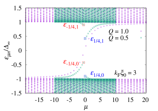
Figure 5: (Color online) Excitation modes around an HFQV for $k_{F}\xi_{0}=3.0$. The cutoff distance of a superconducting disk is $r_{c}=25\xi_{0}$.

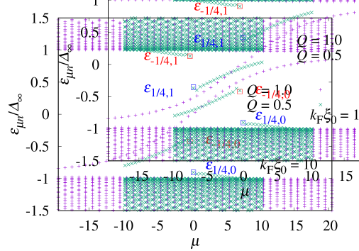
Figure 6: (Color online) Excitation modes around an HFQV for $k_{F}\xi_{0}=10.0$. The cutoff distance of a superconducting disk is $r_{c}=25\xi_{0}$.

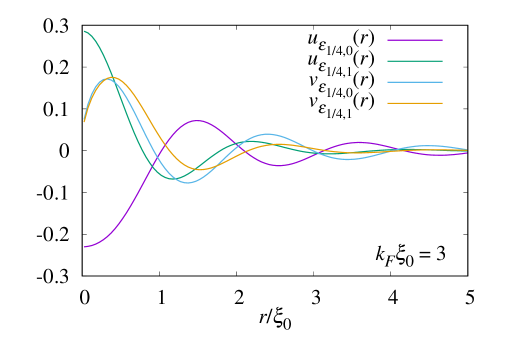
Figure 7: (Color online) Eigenfunctions of the Bogoliubov equation for an HFQV for $\mu=1/4$ with $n=0$ and 1 where $k_{F}\xi_{0}=3.0$ and the cutoff distance of an SC disk is $r_{c}=25\xi_{0}$. The wave function for $\varepsilon_{1/4,0}$ corresponds to the anomalous negative energy state with positive angular momentum.

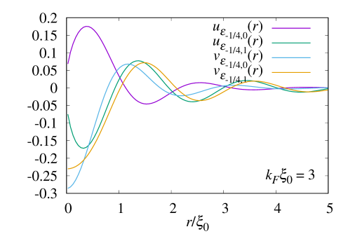
Figure 8: (Color online) Eigenfunctions of the Bogoliubov equation for an HFQV for $\mu=-1/4$ with $n=0$ and 1 where $k_{F}\xi_{0}=3.0$ and the cutoff distance of an SC disk is $r_{c}=25\xi_{0}$. The wave function for $\varepsilon_{-1/4,1}$ corresponds to the anomalous positive energy state with negative angular momentum.

Phase change across the kink When $Y(\theta)$ is a general function of $\theta$, the equation for the radial function $g(r)$ is written as

$$\sigma_{3}\frac{\hbar^{2}}{2m}\Bigg{[}-\frac{\partial^{2}g}{\partial r^{2}}-\frac{1}{r}\frac{\partial g}{\partial r}+\hat{M}\frac{1}{r^{2}}g-k_{F}^{2}g\Bigg{]}+\left(\begin{array}[]{cc}0&e^{-iYQ}\\ e^{iYQ}&0\\ \end{array}\right)$$ (40)

$$~{}~{}~{}\times\Delta_{0}(r)g=\epsilon_{\mu n}g.$$ (41)

When $Y=0$, the potential term equals $\Delta_{0}(r)g$, while the potential term becomes $-\Delta_{0}(r)g$ when $Y=2\pi$ with the change of sign for $Q=1/2$. As $Y$ changes from 0 to $2\pi$, the phase of $\tilde{u}_{\mu n}$ changes by $\pi$ and and that of $\tilde{v}_{\mu n}$ remains the same. This is shown in Figs. 9 and 10. Thus the wave function is defined on a Riemann surface where two planes are connected on the kink as the Riemann surface of complex function $w=z^{1/2}$ with $z=x+iy$.

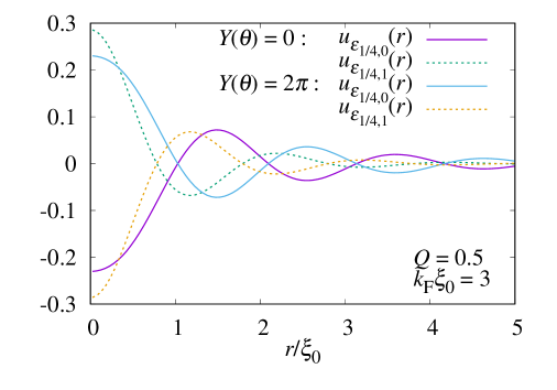
Figure 9: (Color online) Eigenfunction $u$ of the Bogoliubov equation for an HFQV for $Y=0$ and $Y=2\pi$ with $\mu=1/4$, $n=0$ and 1 where $k_{F}\xi_{0}=3.0$ and the cutoff distance of an SC disk is $r_{c}=25\xi_{0}$.

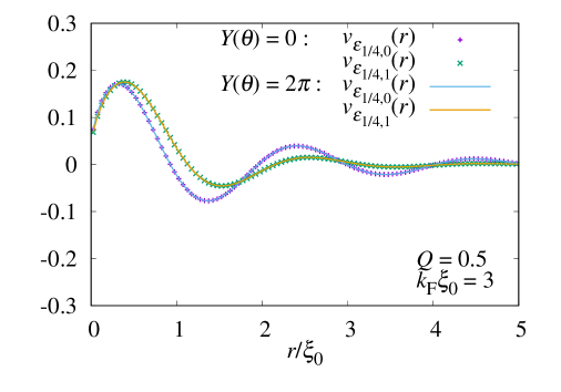
Figure 10: (Color online) Eigenfunction $v$ of the Bogoliubov equation for an HFQV for $Y=0$ and $Y=2\pi$ with $\mu=1/4$, $n=0$ and 1 where $k_{F}\xi_{0}=3.0$ and the cutoff distance of an SC disk is $r_{c}=25\xi_{0}$.

5 Topological Index with Boundary and Fractional Skyrmion Number

Topological index with boundary The skyrmion number (or Chern number) is the topological number that can be assigned to a vortex. Usually this number is an integer for a vortex with integer vorticity, which is related with property that the Andreev bound state exists near zero energy. We show that the topological numer is fractional for an FFQV. We write the Hamiltonian in the form,

$$H =\epsilon(x,y)\sigma_{3}+\Delta_{0}(r)\cos(Q\phi)\sigma_{1}+\Delta_{0}(r)\sin(Q\phi)\sigma_{2}$$

$$=E(x,y)\left(n_{3}\sigma_{3}+n_{1}\sigma_{1}+n_{2}\sigma_{2}\right),$$ (42)

where $E(x,y)=\sqrt{\epsilon(x,y)^{2}+\Delta_{0}(r)^{2}}$. ${\bf n}\equiv(n_{1},n_{2},n_{3})$ is a vector of unit length: $n_{1}^{2}+n_{2}^{2}+n_{3}^{2}=1$. Immediately we can define the topological number associated with ${\bf n}$,

$$N\equiv\frac{1}{4\pi}\int{\bf n}\cdot\left(\frac{\partial{\bf n}}{\partial x}\times\frac{\partial{\bf n}}{\partial y}\right)dxdy.$$ (43)

Whether $N$ is an integer or not is dependent on the boundary condition for $(\theta,Q\phi)$. Let us consider an HFQV with $Q=1/2$. The angle variable $\theta$ is given by $\theta=\tan^{-1}(x/y)$, and when $\theta$ varies from 0 to $2\pi$, $Q\phi$ varies from 0 to $\pi$. $Q\phi=\phi/2$ is parametrized as

$$\sin\left(Q\phi\right) =\frac{1}{2i}\left(\left(\frac{z}{r}\right)^{Q}-\left(\frac{\bar{z}}{r}\right)^{Q}\right),$$ (44)

$$\cos\left(Q\phi\right) =\frac{1}{2}\left(\left(\frac{z}{r}\right)^{Q}+\left(\frac{\bar{z}}{r}\right)^{Q}\right),$$ (45)

for $z=x+iy$ and its complex conjugate $\bar{z}=x-iy$. When the point $(x,y)$ moves on the entire plane for $0<\theta<2\pi$, $(\theta,Q\phi)$ covers half of the sphere $S^{2}$.

For an HFQV, we have two contributions $N=N_{vortex}+N_{kink}$ from the regions $R=\{\delta<\theta<2\pi-\delta\}$ and $\partial R=\{-\delta<\theta<\delta\}$ for small positive $\delta$, respectively. We can write $N_{vortex}=N_{bulk}$ and $N_{kink}=N_{boundary}$. We define the angle $\varphi$ by $\cos\varphi=\epsilon/\sqrt{\epsilon^{2}+\Delta_{0}^{2}}$ and $\sin\varphi=\Delta_{0}/\sqrt{\epsilon^{2}+\Delta_{0}^{2}}$. Then we have

$$N_{vortex} =\frac{Q}{4\pi}\int_{\theta\in R}\sin\varphi\left(\frac{\partial\varphi}{\partial x}\frac{\partial\phi}{\partial y}-\frac{\partial\varphi}{\partial y}\frac{\partial\phi}{\partial x}\right)dx\wedge dy$$

$$=\frac{Q}{2}\int\frac{\Delta_{0}^{2}}{(\epsilon^{2}+\Delta_{0}^{2})^{3/2}}d\epsilon=Q=\frac{1}{2},$$ (46)

where we assume that $\epsilon$ takes the value $-\infty<\epsilon<\infty$ and $d\epsilon/dr\geq 0$. $N_{vortex}$ is regarded as the skyrmion number for the vortex. When $\theta\in\partial R$, we use $d\phi/d\theta=2\pi\delta(\theta)$ so that we obtain

$$N_{kink}=\frac{Q}{4\pi}\int_{\theta\in\partial R}\sin\varphi\frac{\partial\varphi}{\partial r}2\pi\delta(\theta)dr\wedge d\theta=Q=\frac{1}{2}.$$ (47)

The total index $N$ is given by

$$N=N_{vortex}+N_{kink}=1.$$ (48)

This indicates that the topological number is divided into two contributions from the vortex and the kink (boundary). This is the reason why the vortex has the fractional topological number. This may be regarded as a kind of the index theorem for manifolds with boundary[51, 52, 53].

Skyrmion on a Riemann surface This is generalized for general rational $Q$, where we have

$$N_{vortex}=Q.$$ (49)

Thus the topological number $N_{vortex}$ is a fractional number for an FFQV. An FFQV can be regarded as a skyrmion on a Riemann surface. For an HFQV, $\phi$ is defined on the Riemann surface defined by the function $w=z^{1/2}$. The Riemann surface $w=z^{1/2}$ is identical to $S^{2}$ by compactification, which induces a map $S^{2}\rightarrow S^{2}$. The topological number $N_{vortex}$ is the winding number of this map. Thus $N_{vortex}$ calculated on the Riemann surface is $N_{vortex}=1$. $N_{vortex}$ for an HFQV corresponds to the integration on one sheet and this results in $N_{vortex}=1/2$.

Non-abelian statistics of fractional-quantum vortices We argue that fractional-quantum vortices follow non-abelian statistics. Suppose that an FFQV goes around the other FFQV in the counterclockwise direction. The phase of an electron and a hole in the FFQV changes $Q\pi$ and $-Q\pi$, respectively. For an HFQV, the wave function takes phase factors $i$ and $-i$ for electrons and holes, respectively. Then the Bogoliubov operator is transformed to the other operator in the process of exchange of HFQVs and the Bogoliubov amplitudes are transformed as

$$\left(\begin{array}[]{c}u\\ v\\ \end{array}\right)\rightarrow\left(\begin{array}[]{c}u\\ -v\\ \end{array}\right).$$ (54)

This indicates that two HFQVs follow non-abelian statistics. This differs from the non-abelian statistics in p-wave superconductors[54].

6 Discussion

We have investigated quasi-particle excitation modes in a half-flux quantum vortex by solving the Bogoliubov equation numerically. We have found that there is no low-lying Andreev bound state near zero energy in the vortex core, that is, there is the energy region where no Andreev bound states exist. The skyrmion number $N_{vortex}$ becomes fractional for an FFQV. An HFQV is nothing but a half-skyrmion. The index $N_{kink}$ is just the boundary contribution, and $N_{vortex}=N_{bulk}$ becomes fractional due to this: $N_{vortex}=N-N_{kink}$.

We discuss scanning tunneling microscope (STM) observations of HFQV here. It is important that the existence of HFQV will be confirmed by measurements by STM measurements because the quasiparticle spectra are different between HFQVs and conventional vortices. The phase of $\tilde{u}$ takes two values 0 or $\pi$ depending on which side of the Riemann surface the quasiparticle lies. The density of states depends on $|\tilde{u}|^{2}$ and $|\tilde{v}|^{2}$ and is independent of the phase of $\tilde{u}$. Thus scanning tunneling spectroscopy (STS) results will not depend on the plane of the Riemann surface of the phase of $\tilde{u}$.

Acknowledgment This work was supported in part by Grant-in-Aid from the Ministry of Education, Culture, Sports and Science (MEXT) of Japan (No. 17K05559).

References

- [1] V. A. Moskalenko: Fiz. Metal and Metallored 8, 2518 (1959).
- [2] H. Suhl, B. T. Mattis and L. W. Walker: Phys. Rev. Lett. 3, 552 (1959).
- [3] J. Peretti, Phys. Lett. 2, 275 (1962).
- [4] J. Kondo: Prog. Theor. Phys. 29, 1 (1963).
- [5] V. Stanev and Z. Tesanovic, Phys. Rev. B81, 134522 (2010).
- [6] Y. Tanaka and T. Yanagisawa, J. Phys. Soc. Jpn. 79, 114706 (2010).
- [7] Y. Tanaka and T. Yanagisawa, Solid State Commun. 150, 1980 (2010).
- [8] R. G. Dias and A. M. Marques, Supercond. Sci. Technol. 24, 085009 (2011).
- [9] T. Yanagisawa, Y. Tanaka, I. Hase and K. Yamaji, J. Phys. Soc. Jpn. 81, 024712 (2012).
- [10] X. Hu and Z. Wang, Phys. Rev. B85, 064516 (2012).
- [11] V. Stanev, Phys. Rev. B85, 174520 (2012).
- [12] C. Platt, R. Thomale, C. Homerkamp and S. C. Zhang, Phys. Rev. B85, 180502 (2012).
- [13] S. Maiti and A. V. Chubukov, Phys. Rev. B87, 144511 (2013).
- [14] B. J. Wilson and M. P. Das, J. Phys. Condens. Matter 25, 425702 (2013).
- [15] R. Ganesh, G. baskaran, J. van den Brink and D. V. Efremov, Phys. Rev. Lett. 113, 177001 (2014).
- [16] Y. S. Yerin, A. N. Omelyanchouk and E. Il’ichev, Super. Sci. Technol. 28, 095006 (2015).
- [17] T. Yanagisawa and I. Hase, J. Phys. Soc. Jpn. 82, 124704 (2013).
- [18] S. Z. Lin and X. Hu, New J. Phys. 14, 063021 (2012).
- [19] K. Kobayashi, Y. Ota, M. Machida and H. Aoki, Phys. Rev. B88, 224516 (2013).
- [20] T. Koyama, J. Phys. Soc. Jpn. 83, 074715 (2014).
- [21] T. Yanagisawa and Y. Tanaka, New J. Phys. 16, 123014 (2014).
- [22] Y. Tanaka, I. Hase, T. Yanagisawa, G. Kato, T. Nishio and S. Arisawa, Physica C516, 10 (2015).
- [23] S. G. Sharapov, V. P. Gusynin and H. Beck, Eur. Phys. J. B39, 062001 (2002).
- [24] T. Yanagisawa, J. Phys. Soc. Jpn. 86, 104711 (2017).
- [25] Yu. A. Izyumov and V. M. Laptev, Phase Transitions 20, 95 (1990).
- [26] G. E. Volovik, The Universe in a Helium Droplet (Oxford University Press, Oxford, 2009).
- [27] Y. Tanaka: Phys. Rev. Lett. 88, 017002 (2001).
- [28] E. Babaev, Phys. Rev. Lett. 89, 067001 (2002).
- [29] A. D. Col, V. B. Geshkenbein, and G. Blatter, Phys. Rev. Lett. 94, 097001 (2005).
- [30] H. Bluhm, N. C. Koshnick, M. E. Huber and K. A. Moler, Phys. Rev. Lett. 97, 237002 (2006).
- [31] J. Goryo, S. Soma, and H. Matsukawa, Europhys. Lett. 80, 17002 (2007).
- [32] L. F. Chibotaru and V. H. Dao, Phys, Rev. B81, 020502 (2010).
- [33] S. V. Kuplevakhsky, A. N. Omelyanchouk and Y. S. Yerin, Low Temp. Phys. 37, 667 (2011).
- [34] J. Garaud, J. Carlstrom and E. Babaev, Phys. Rev. Lett. 107, 197001 (2011).
- [35] J. C. Pina, C. C. de Souza Silva, and M. V. Miloevic, Phys. Rev. B86, 024512 (2012).
- [36] J. Garaud, J. Carlstrom, E. Babaev and M. Speight, Phys. Rev. B87, 014507 (2013).
- [37] J. Smiseth, E. Smorgrav, E. Babaev and A. Sudbo, Phys. Rev. B71, 214509 (2005).
- [38] Y. Tanaka, H. Yamamori, T. Yanagisawa, T. Nishio, S. Arisawa, Physica C548, 44 (2018).
- [39] M. Hayashi, J. Phys. Soc. Jpn. 88, 035002 (2019).
- [40] Y. Nagai and Y. Kato, J. Phys. Soc. Jpn. 88, 054707 (2019).
- [41] H. Y. Choi, J. H. Yun, Y. Bang and H. C. Lee, Phys. Rev. B80, 052505 (2009).
- [42] P. M. Shirage, K. Kihou, K. Miyazawa, C.-H. Lee, H. Kito, H. Eisaki, T. Yanagisawa, Y. Tanaka and A. Iyo, Phys. Rev. Lett. 103, 257003 (2009).
- [43] T. Yanagisawa, K. Odagiri, I. Hase, K. Yamaji, P. M. Shirage, Y. Tanaka, A. Iyo and H. Eisaki, J. Phys. Soc. Jpn. 78, 094718 (2009).
- [44] S. M. M. Virtanen and M. M. Salomaa, Phys. Rev. B60, 14581 (1999).
- [45] T. Yanagisawa, I. Hase, and Y. Tanaka, Phys. Lett. A382, 3483 (2018).
- [46] C. Caroli, P. G. de Gennes and J. Matricon, Phys. Lett. 9, 307 (1964).
- [47] P. G. de Gennes, Superconductivity of Metals and Alloys (W. A. Benjamin, New York, 1966).
- [48] G. E. Volovik, JETP Lett. 70, 609 (1999).
- [49] I. O. Kulik, Sov. Phys. JETP 30, 844 (1970).
- [50] M. Stone, Phys. Rev. B54, 13222 (1996).
- [51] M. F. Atiyah, V. K. Patodi, and I. M. Singer, Math. Proc. Cambridge Philos. Soc. 77, 43 (1975).
- [52] R. B. Melrose, The Atiyah-Patodi-SInger Index Theorem (Taylor & Francis, Milton Park, UK, 1993).
- [53] H. Fukaya, T. Onogi, and S. Yamaguchi, Phys. Rev. D 96, 125004 (2017).
- [54] D. A. Ivanov, Phys. Rev. Lett. 86, 268 (2001).