Beyond image classification: zooplankton identification with deep vector space embeddings

Abstract

Zooplankton images, like many other real world data types, have intrinsic properties that make the design of effective classification systems difficult. For instance, the number of classes encountered in practical settings is potentially very large, and classes can be ambiguous or overlap. In addition, the choice of taxonomy often differs between researchers and between institutions. Although high accuracy has been achieved in benchmarks using standard classifier architectures, biases caused by an inflexible classification scheme can have profound effects when the output is used in ecosystem assessments and monitoring.

Here, we propose using a deep convolutional network to construct a vector embedding of zooplankton images. The system maps (embeds) each image into a high-dimensional Euclidean space so that distances between vectors reflect semantic relationships between images. We show that the embedding can be used to derive classifications with comparable accuracy to a specific classifier, but that it simultaneously reveals important structures in the data. Furthermore, we apply the embedding to new classes previously unseen by the system, and evaluate its classification performance in such cases.

Traditional neural network classifiers perform well when the classes are clearly defined a priori and have sufficiently large labeled data sets available. For practical cases in ecology as well as in many other fields this is not the case, and we argue that the vector embedding method presented here is a more appropriate approach.

1 Introduction

In classification problems, the goal is to map each input to one of a discrete set of classes. A typical example is labeling images according to objects pictured, e.g., distinguishing pictures of cats from pictures of dogs. The output of a classifier can be a single value, but is often a vector where each element represents the classifier’s confidence that the input belongs to the corresponding class.

Recently, deep neural networks have been used with great success for many classification tasks. Often, these classifiers apply a softmax function (a generalization of the logistic function to multiple outputs) to generate the final output. This scales the output vector so that the scores for the classes sum to one, resembling a set of probabilities for the class assignment.

This approach is commonly used for image classification, where it has been overwhelmingly successful for many benchmark data sets. Yet, it relies on a set of assumptions that can be naive in many practical situations. Here, we will use the classification of zooplankton images to illustrate why a vector space embedding can be a more appropriate approach.

1.1 Zooplankton classification

Plankton constitute a fundamental component of aquatic ecosystems, and since they form the basis for many food chains and also rapidly adapt to changes in the environment, monitoring plankton diversity and abundances is a central input to marine science and management [ICES, 2018].

Imaging systems are being deployed to scale up sampling efforts [Stemmann and Boss, 2012, Benfield et al., 2007], but the manual curation process remains expensive and time consuming [ICES, 2018]. Recently, automated classifiers based on deep neural networks have been developed and applied successfully to benchmark problem sets, but deployment in a practical marine management situation poses some challenges.

For standard classifiers, the set of target classes is an integral part of the structure of the classifier. In other words, the set of target classes must be finite and known in advance. In contrast, plankton communities often consists of surprisingly large numbers of species (e.g., [Huisman and Weissing, 1999, Schippers et al., 2001]), with highly varying abundance. Even if all species were known, many would not be represented in the training data, and the long-tailed abundance distribution poses a challenge to standard methods [Van Horn and Perona, 2017]. A further complication is the various forms of artifacts, including detritus, clusters of multiple specimens, and pieces of fragile plankton that break apart during processing [Benfield et al., 2007].

In addition, different researchers may operate with different taxonomies, or otherwise suffer from inconsistent annotation [Malde et al., 2019]. It is symptomatic that comparing the ZooScan data set used here with another, similar data set [Orenstein et al., 2015] with around 100 classes, we find that only three of the classes are shared. Two of those represent artifacts (bubble and detritus), and only one plankton taxon (coscinodiscus) was present as a class in both data sets. While it is possible to train classifiers separately for each taxonomy, this diminishes the total value of the data and inhibits comparisons and reproducibility.

Several automated systems for plankton classification have been developed and applied to benchmark data sets (e.g, [Luo et al., 2018, Dai et al., 2016, Lee et al., 2016]), but report problems stemming from the severe class imbalance in the data. In addition, image quality is often poor, and image sizes can vary enormously. In practice, automation is still mainly used to aid or supplement a manual curation process [Uusitalo et al., 2016]. For interactive processes, methods that reveal more of the structure of the data are more useful than categorical class assignments [ICES, 2018].

1.2 Vector embeddings as an alternative

Here we explore vector embedding of the input space as an alternative to the standard approach. Each input is mapped to a vector in a high-dimensional space with no a priori relationship between classes and dimensions. Instead, the mapping (or embedding) is constructed to reflect some concept of similarity between inputs. In our case, class membership represents similarity, and the goal of the embedding is to map inputs from the same class to vectors that are close to each other, and inputs belonging to different classes to vectors that are farther apart.

Compared to traditional classification, the embedding models the structure of the input space with high resolution. This is important when the system deals with new classes of inputs. Whether two inputs belong to the same or different classes can be determined solely from the distance between their corresponding vector space embeddings. Similarly, new classes can be constructed based on clusters or other structure in the embedding vector space, without retraining or other modifications to the system.

One application where neural networks that output embeddings have been applied with particular success, is face recognition [Taigman et al., 2014, Schroff et al., 2015]. Not unlike plankton classification, the goal is to identify a large number of classes (for face recognition, each individual person represent one class). Thus we have a classification problem with an unknown, large, and possibly open-ended number of classes, often with very sparse data and poor annotation. As for face recognition, it is important to be able to identify classes from few samples, so called low-shot, one-shot [Fei-Fei et al., 2006], and zero-shot [Larochelle et al., 2008, Yu and Aloimonos, 2010] classification.

Inspired by this, we here apply a vector embedding approach to the task of classifying zooplankton images, and compare the results to using a straightforward classifier based on the Inception v3 [Szegedy et al., 2016] neural network architecture. We show how classes form clusters in the embedding space, discuss confoundings, and explore how the vector embedding performs on previously unseen classes.

2 Methods

2.1 Data set

Recently, a large set of ZooScan [Gorsky et al., 2010, Grosjean et al., 2004] images of plankton was made available to the public [Elineau et al., 2018]. The data set consists of monochromatic images organized into 93 categories, most of them representing zooplankton taxa. In addition, several error categories exist, with names like artefact, detritus, and bubble. Abundances range from the 39 images labeled Ctenophora, up to the 511,700 labeled detritus. Three of the four most abundant categories represent various types of artifact.

The images vary widely in size. We converted the images to a standard size of 299x299 pixels. Smaller images were padded up to this size, while larger images were scaled down. The resized images were then used to construct data sets for training, validation, and testing. For training, we used 65 non-artifact classes with abundances above 500, in addition to bubble. From each class, 100 random images were selected to serve as a validation set, and then another 100 images for the test set. The remaining images constituted the training set.

A second test set consisted of 100 images sampled randomly from each of the 38 classes not represented in the other sets. For the classes with less than 100 images, all images were used.

2.2 Standard neural network classifier

To provide a baseline for achievable classification accuracy, we used the convolutional neural network Inception v3, initialized with weights pre-trained on the ImageNet data set [Deng et al., 2009]. The default 1000-class output layer was replaced with a 65-class softmax output to match the number of classes.

The network was trained using the SGD optimizer with a learning rate of 0.0001 and momentum of 0.9, using a categorical cross-entropy cost function. During training, mean square error and accuracy were reported.

All neural networks were implemented using Keras [Chollet et al., 2015] with a Tensorflow [Abadi et al., 2016] backend, and run on a computer with RTX2080 Ti GPU accelerators (Nvidia Corporation, Santa Clara, California, USA).

2.3 Siamese networks

The particular embedding technique we will investigate here is called siamese networks [Bromley et al., 1994, Hoffer and Ailon, 2015, Wang et al., 2014], in a variant using what is called a triplet loss function. The network is given three inputs, one from a randomly selected class (the anchor), one randomly sampled from the same class (the positive) and a random sample from another class (the negative). The cost function $J$ is designed to reward a small distances from the anchor to the positive and a large distance from the anchor to the negative.

$J(a,p,n)=\max(0,||a-p||^{2}-||a-n||^{2}+\alpha)$

The parameter $\alpha$ serves as a margin to avoid the network learning a trivial, zero-cost solution of embedding all inputs in the same point.

For vector space embedding, we again used Inception v3, but replaced the softmax with a global average pooling layer and a 128-dimensional vector output layer. The output vector was further constrained to unit length, so that the vector embedding results in a point on a hypersphere with a radius of one.

Training was performed using the SGD optimizer and a batch size of 20. The learning rate was set to decay of 0.9 and an initial value of 0.01. The margin parameter $\alpha$ was initially set to 1.0, but raised to 1.3 after 20 iterations, and to 1.5 after 30 iterations.

2.4 Classification from a vector space embedding

A vector space embedding does not directly present a classification, but we can use any of a number of methods suitable for euclidean spaces. An advantage of vector space embeddings is to allow the use of unsupervised methods, and when no known data is available, classes can be determined using standard approaches like $k$-means clustering.

Here, we will compare classifications in the embedding space using two simple supervised methods. First, using data with known classes we calculate the centroids for each class and assign new data to the class represented by the closest centroid. Alternatively, we use nearest neighbor classification (kNN, using the approximative algorithm BallTree from Scikit-learn [Pedregosa et al., 2011]) against data with known classifications.

3 Results

3.1 Baseline classification

Inception v3 was trained for 220 epochs on the 65-class training data set, the metrics are shown in Fig. 1. The classifier reaches 80% accuracy on validation data after 67 epochs, and appears to converge to approximately 86% accuracy after around 150 epochs.

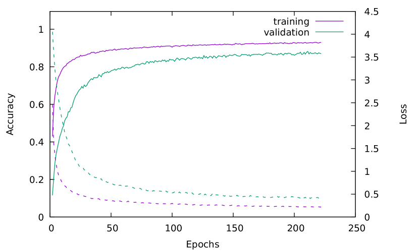
Figure 1: Training Inception v3 for plankton classification. The loss (solid) and accuracy (dashed) for training (purple) and validation (green) data are shown as training progresses.

We select the classifier trained for 200 epochs, and use it to classify the test set. Total accuracy was 87.7%, a table with more detailed results for the different classes can be found as supplementary information.

3.2 Training the vector embedding

For validation, we calculated the centroid of the embeddings for each category of plankton. We define the cluster radius to be the average distance from the centroid for each image in the validation set. During training, we calculate the cluster radius (Suppl. Fig 1) and the change in centroid (Suppl. Fig 2) for every class in the training set. As training progresses, cluster radii shrink, while the magnitude of the changes to the embedding decreases. In some cases, large magnitude changes affect many or all clusters simultaneously, indicating larger scale rearrangements in the embedding.

We can also check if we are able to correctly predict the correct class by assigning each image to the closest centroid. The results are shown in Suppl Fig. 3. Both analyses show rapid improvement for 10 iterations, slower gains the next 20, and only small improvements after 30 iterations. In the following, we use the network trained for 30 iterations to construct the vector embeddings.

3.3 Clusters in the embedding space

As training progresses, clusters start to emerge in the embedding space. A t-SNE [Maaten and Hinton, 2008] rendering is shown in Fig. 2, where the structure of the input data is evident.

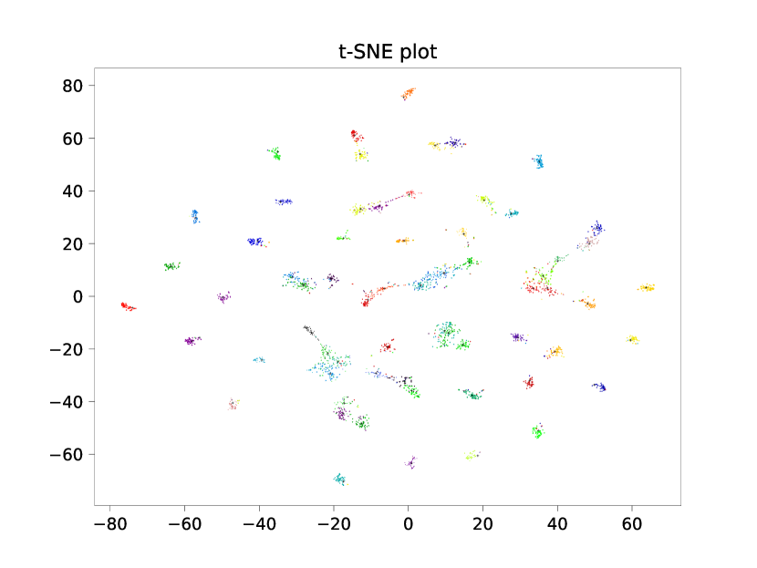
Figure 2: The data projected into the embedding space and displayed using a t-SNE rendering. Class centroids are marked by black crosses.

3.4 Classification in the embedding space

For classification using kNN, we investigate possible choices for the parameter $k$. We split the validation data set in two (50 instances for each class in each partition), and used one partition as a reference to classify the other. Experimenting with different values of $k$ indicates that $k=10$ might be a good value to use (see supplementary figure).

Fig. 3 shows the F1 scores using the default classifier on the whole data set. In addition, we show the centroid-based classification in the embedded space and kNN classification using various values of $k$, splitting the test set into equal partitions for reference and an evaluation.

We see that performance is comparable across most classes, but there are some classes where the standard classifier gives different performance from the embedding. The standard classifier outperforms the embedding for nauplii__Cursacea (class 65, F1 scores of 0.93 and 0.69) and nauplii__Cirripedia (class 12, F1 0.97 and 0.51). A substantial difference is also observed for egg__Cavolinia_inflexa (class 64, F1 0.93 and 0.33) and egg__Actinopterygii (class 17, F1 0.94 and 0.70). In contrast, the embedding has better performance for Calanoida (class 36, F1 0.50 and 0.96) and larvae__Crustacea (class 36, F1 0.62 and 0.84).

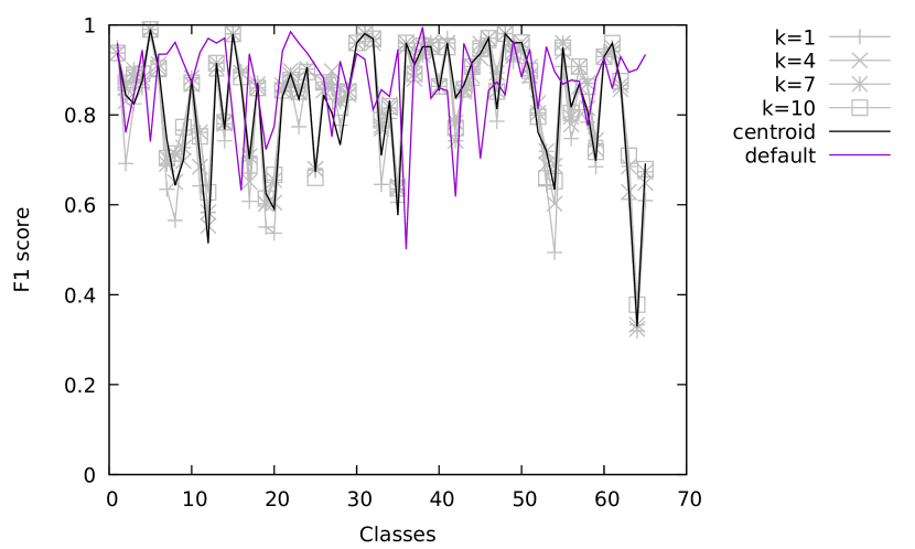
Figure 3: F1-scores across classes in the test set for centroid-based classification in black and kNN using various values for $k$ in gray. The standard classifier perfomance is shown in purple.

To elucidate the misclassifications, the ten most commonly occurring confoundings with kNN ($k=10$) are shown in Table 1.

Table 1: Commonly seen confoundings in the test data set.

True class	Predicted class	rate
tail__Appendicularia	tail__Chaetognatha	0.380
Oncaeidae	Harpacticoida	0.260
Chaetognatha	tail__Chaetognatha	0.260
Euchaetidae	Candaciidae	0.220
Eucalanidae	Rhincalanidae	0.200
Harpacticoida	Oncaeidae	0.180
nectophore__Diphyidae	gonophore__Diphyidae	0.180
Rhincalanidae	Eucalanidae	0.180
Centropagidae	Euchaetidae	0.160
Limacidae	Limacinidae	0.160

Not unexpectedly, confoundings occur between classes of organism fragments or parts. The most commonly occurring confounding consists of the two classes of tails, and confounding Chaetognatha with the class of its tails is the third most common occurrence (see also Fig. 4, middle row). In addition, species are confounded with their different stages, e.g., we see confounding between different forms of the Diphyidae species (Fig. 4, top row).

We also see pairs of similar species being confounded with each other (e.g., Oncaeidae with Harpacticoida, and Eucalanidae with Rhincalanidae).

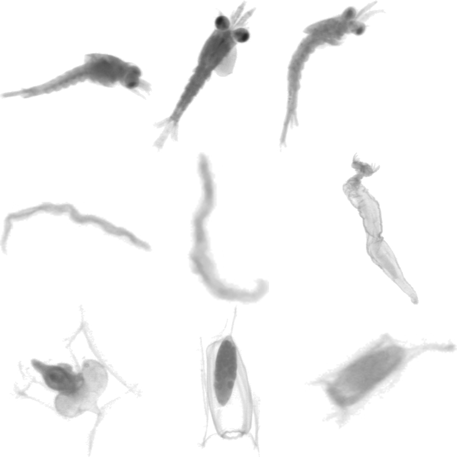
Figure 4: Example of plankton images that are difficult to resolve. Upper row, from the left: Decapoda, zooa__Decapoda, and larvae__Crustacea. Middle row: tail__Appendicularia, tail__Chaetognatha, and Chaetognatha. Second row shows variants of Abylopsis, from the left: eudoxie, gonophore, and nectophore.

3.5 Previously unseen classes

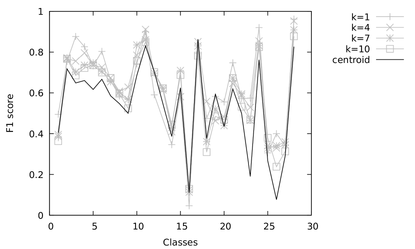
Figure 5: F1-scores across classes for centroid-based classification (black) and kNN using various values for $k$ (gray).

For the previously unseen classes, we use the same approach of dividing the test set in two and using one part for reference and the other for evaluation. The results are shown in Fig. 3. Here we see that performance is highly variable. Using centroid classification, the highest performing classes were Rhopalonema (number 17, F1 0.86), badfocus_artifact (number 28, F1 0.82), and egg_other (number 11, 0.83). The lowest scoring classes were Euchirella (number 26, F1 0.07), Aglaura (number 23, 0.19), and multiple__other (number 27, F1 0.29). Several low performing classes are caused by confusing the Abylopsis_tetragona variants (number 14, gonophore, F1 0.38, number 16 eudoxie, F1 0.11, and number 25, nectophore, F1 0.26). kNN classifications outperforms centroids slightly for several classes, but the overall picture remains the same.

Table 2: Commonly seen confoundings in previously unseen classes.

True class	Predicted class	rate
eudoxie__Abylopsis_tetrag	nectophore__Abylopsis_tet	0.320
Scyphozoa	ephyra	0.280
Rhopalonema	Aglaura	0.260
gonophore__Abylopsis_tetr	nectophore__Abylopsis_tet	0.240
Calocalanus pavo	Euchirella	0.240
nectophore__Abylopsis_tet	eudoxie__Abylopsis_tetrag	0.220
badfocus__artefact	detritus	0.200
Calocalanus pavo	part__Copepoda	0.180
Echinoidea	larvae__Annelida	0.180
artefact	badfocus__artefact	0.180

Again we see that a large fraction of the confoundings occur between variants of species, in particular Abylopsis tetragona (Fig. 4, bottom row). In addition, there is several cases of confounding between artifact classes.

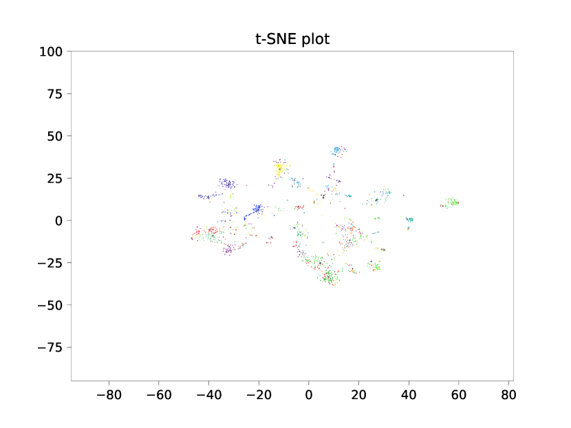
Figure 6: A t-SNE rendering of the data in the unseen classes after 30 iterations.

4 Discussion

Using the average F1 score over the classes, the standard deep learning classifier achieves a score of 0.87 on the data set. Using our vector space embedding and classifying using kNN (k=10), we achieve a score of 0.84. The standard classifier thus outperforms the embedding, but not by a large margin.

Interestingly, the vector space embedding performs better on several classes. The standard classifier often mislabels many species as Calanoida, resulting in a low F1 score of 0.50, while the embedding classifier achieves an F1 score of 0.96 for this class. In contrast, the standard classifier appears to be better at precisely separating classes with very similar morphology, for instance classes of eggs or nauplii. As similar classes are embedded close to each other, they are more difficult to differentiate. Although the proximity is semantically meaningful, this reduces accuracy somewhat. For maximizing absolute classification performance, an ensemble using both methods is likely to be optimal.

In contrast to classification, the embedding is able to better capture the underlying structure of the data. This has many potential uses, for instance to identify misclassified data, or to allow switching to a different taxonomy. In this way, the embedding can be used actively to evaluate and even refine the choice of classes used.

As a more challenging test case, we applied the embedding approach to data in classes not present in the training data. Here we achieve a more modest performance, with an average F1 score of 0.61. Some of the classes gave particularly poor results, while other classes were accurately identified. Even for classes where performance is too low to be used directly, the information provided by the embedding can guide and accelerate manual or semi-interactive processing. We believe training with more diverse data is likely to improve generality of the embedding.

The use of very simple schemes used to compare classification performance in the embedding space (i.e., centroid clustering and kNN) is a deliberate choice. More complex schemes may be able to give better classification performance, but our goal here is to emphasize the ability of the embedding to capture the structure of the input. Using a complex non-linear classifier on the embedding vectors would defeat this purpose, since it would be more difficult to separate complexity captured by the embedding from complexity captured by the final classification stage.

5 Conclusions

Classification of zooplankton is an important task, but the inherent complexity and other limitations of the data requires more flexibility than that provided by standard classifiers. Earlier attempts have successfully been able to classify benchmark data sets [Py et al., 2016, Lee et al., 2016], but achieve high accuracy at the expense of removing low abundance or otherwise difficult classes [Luo et al., 2018].

Here we have shown that using a deep learning vector space embedding, we can model important structure in the data, while retaining the flexibility to perform classification with accuracy comparable to state of the art classifiers.

6 Author’s contributions

KM conceived of the ideas and methodology and led the writing of the manuscript, HK implemented benchmarks and visualizations of the results. Both authors contributed critically to the draft and approved of its publication.

7 Availability

The data set and software used here is publicly available as described above. Source code for network construction, training, and analysis can be found as GitHub repositories at

https://github.com/ketil-malde/plankton-siamese and https://github.com/ketil-malde/plankton-learn

An interactive rendering of the data sets and classifications using https://projector.tensorflow.org/ can be found here:

https://projector.tensorflow.org/?config=https://home.malde.org/vector_embeddings/

References

- [Abadi et al., 2016] Abadi, M., Barham, P., Chen, J., Chen, Z., Davis, A., Dean, J., Devin, M., Ghemawat, S., Irving, G., Isard, M., et al. (2016). Tensorflow: A system for large-scale machine learning. In 12th USENIX Symposium on Operating Systems Design and Implementation (OSDI 16), pages 265–283.
- [Benfield et al., 2007] Benfield, M. C., Grosjean, P., Culverhouse, P. F., Irigoien, X., Sieracki, M. E., Lopez-Urrutia, A., Dam, H. G., Hu, Q., Davis, C. S., Hansen, A., et al. (2007). Rapid: research on automated plankton identification. Oceanography, 20(2):172–187.
- [Bromley et al., 1994] Bromley, J., Guyon, I., LeCun, Y., Säckinger, E., and Shah, R. (1994). Signature verification using a” siamese” time delay neural network. In Advances in neural information processing systems, pages 737–744.
- [Chollet et al., 2015] Chollet, F. et al. (2015). Keras. https://keras.io.
- [Dai et al., 2016] Dai, J., Wang, R., Zheng, H., Ji, G., and Qiao, X. (2016). Zooplanktonet: Deep convolutional network for zooplankton classification. In OCEANS 2016-Shanghai, pages 1–6. IEEE.
- [Deng et al., 2009] Deng, J., Dong, W., Socher, R., Li, L.-J., Li, K., and Fei-Fei, L. (2009). Imagenet: A large-scale hierarchical image database. In 2009 IEEE conference on computer vision and pattern recognition, pages 248–255. Ieee.
- [Elineau et al., 2018] Elineau, A., Desnos, C., Jalabert, L., Olivier, M., Romagnan, J.-B., Brandao, M., Lombard, F., Llopis, N., Courboulès, J., Caray-Counil, L., Serranito, B., Irisson, J.-O., Picheral, M., Gorsky, G., and Stemmann, L. (2018). Zooscannet: plankton images captured with the zooscan.
- [Fei-Fei et al., 2006] Fei-Fei, L., Fergus, R., and Perona, P. (2006). One-shot learning of object categories. IEEE transactions on pattern analysis and machine intelligence, 28(4):594–611.
- [Gorsky et al., 2010] Gorsky, G., Ohman, M. D., Picheral, M., Gasparini, S., Stemmann, L., Romagnan, J.-B., Cawood, A., Pesant, S., García-Comas, C., and Prejger, F. (2010). Digital zooplankton image analysis using the zooscan integrated system. Journal of plankton research, 32(3):285–303.
- [Grosjean et al., 2004] Grosjean, P., Picheral, M., Warembourg, C., and Gorsky, G. (2004). Enumeration, measurement, and identification of net zooplankton samples using the zooscan digital imaging system. ICES Journal of Marine Science, 61(4):518–525.
- [Hoffer and Ailon, 2015] Hoffer, E. and Ailon, N. (2015). Deep metric learning using triplet network. In International Workshop on Similarity-Based Pattern Recognition, pages 84–92. Springer.
- [Huisman and Weissing, 1999] Huisman, J. and Weissing, F. J. (1999). Biodiversity of plankton by species oscillations and chaos. Nature, 402(6760):407.
- [ICES, 2018] ICES (2018). WKMLEARN: Report of the workshop on machine learning in marine science. Technical Report ICES CM 2018/EOSG:20, International Council for Exploration of the Seas.
- [Larochelle et al., 2008] Larochelle, H., Erhan, D., and Bengio, Y. (2008). Zero-data learning of new tasks. In AAAI, volume 1, page 3.
- [Lee et al., 2016] Lee, H., Park, M., and Kim, J. (2016). Plankton classification on imbalanced large scale database via convolutional neural networks with transfer learning. In 2016 IEEE international conference on image processing (ICIP), pages 3713–3717. IEEE.
- [Luo et al., 2018] Luo, J. Y., Irisson, J.-O., Graham, B., Guigand, C., Sarafraz, A., Mader, C., and Cowen, R. K. (2018). Automated plankton image analysis using convolutional neural networks. Limnology and Oceanography: Methods, 16(12):814–827.
- [Maaten and Hinton, 2008] Maaten, L. v. d. and Hinton, G. (2008). Visualizing data using t-sne. Journal of machine learning research, 9(Nov):2579–2605.
- [Malde et al., 2019] Malde, K., Handegard, N. O., Eikvil, L., and Salberg, A.-B. (2019). Machine intelligence and the data-driven future of marine science. ICES Journal of Marine Science.
- [Orenstein et al., 2015] Orenstein, E. C., Beijbom, O., Peacock, E. E., and Sosik, H. M. (2015). Whoi-plankton- A large scale fine grained visual recognition benchmark dataset for plankton classification. CoRR, abs/1510.00745.
- [Pedregosa et al., 2011] Pedregosa, F., Varoquaux, G., Gramfort, A., Michel, V., Thirion, B., Grisel, O., Blondel, M., Prettenhofer, P., Weiss, R., Dubourg, V., Vanderplas, J., Passos, A., Cournapeau, D., Brucher, M., Perrot, M., and Duchesnay, E. (2011). Scikit-learn: Machine learning in Python. Journal of Machine Learning Research, 12:2825–2830.
- [Py et al., 2016] Py, O., Hong, H., and Zhongzhi, S. (2016). Plankton classification with deep convolutional neural networks. In 2016 IEEE Information Technology, Networking, Electronic and Automation Control Conference, pages 132–136. IEEE.
- [Schippers et al., 2001] Schippers, P., Verschoor, A. M., Vos, M., and Mooij, W. M. (2001). Does “supersaturated coexistence” resolve the “paradox of the plankton”? Ecology letters, 4(5):404–407.
- [Schroff et al., 2015] Schroff, F., Kalenichenko, D., and Philbin, J. (2015). Facenet: A unified embedding for face recognition and clustering. In Proceedings of the IEEE conference on computer vision and pattern recognition, pages 815–823.
- [Stemmann and Boss, 2012] Stemmann, L. and Boss, E. (2012). Plankton and particle size and packaging: from determining optical properties to driving the biological pump. Annual Review of Marine Science, 4:263–290.
- [Szegedy et al., 2016] Szegedy, C., Vanhoucke, V., Ioffe, S., Shlens, J., and Wojna, Z. (2016). Rethinking the inception architecture for computer vision. In Proceedings of the IEEE conference on computer vision and pattern recognition, pages 2818–2826.
- [Taigman et al., 2014] Taigman, Y., Yang, M., Ranzato, M., and Wolf, L. (2014). Deepface: Closing the gap to human-level performance in face verification. In Proceedings of the IEEE Conference on Computer Vision and Pattern Recognition, pages 1701–1708.
- [Uusitalo et al., 2016] Uusitalo, L., Fernandes, J. A., Bachiller, E., Tasala, S., and Lehtiniemi, M. (2016). Semi-automated classification method addressing marine strategy framework directive (msfd) zooplankton indicators. Ecological indicators, 71:398–405.
- [Van Horn and Perona, 2017] Van Horn, G. and Perona, P. (2017). The devil is in the tails: Fine-grained classification in the wild. arXiv preprint arXiv:1709.01450.
- [Wang et al., 2014] Wang, J., Song, Y., Leung, T., Rosenberg, C., Wang, J., Philbin, J., Chen, B., and Wu, Y. (2014). Learning fine-grained image similarity with deep ranking. In Proceedings of the IEEE Conference on Computer Vision and Pattern Recognition, pages 1386–1393.
- [Yu and Aloimonos, 2010] Yu, X. and Aloimonos, Y. (2010). Attribute-based transfer learning for object categorization with zero/one training example. In European conference on computer vision, pages 127–140. Springer.