A computational framework for two-dimensional random walks with restarts

Abstract

The treatment of two-dimensional random walks in the quarter plane leads to Markov processes which involve semi-infinite matrices having Toeplitz or block Toeplitz structure plus a low-rank correction. We propose an extension of the framework introduced in [Math. Comp., 87(314):2811–2830, 2018] which allows to deal with more general situations such as processes involving restart events. This is motivated by the need for modeling processes that can incur in unexpected failures like computer system reboots. We present a theoretical analysis of an enriched Banach algebra that, combined with appropriate algorithms, enables the numerical treatment of these problems. The results are applied to the solution of bidimensional Quasi-Birth-Death processes with infinitely many phases which model random walks in the quarter plane, relying on the matrix analytic approach. The reliability of our approach is confirmed by extensive numerical experimentation on several case studies.

1 Introduction

The treatment of the infinite data structures arising from Markov processes usually relies on the assumption that jumps between states become unlikely when their mutual distance increases. For instance, this is natural when considering random walks on lattices where the particle is forced to move to nearby positions at each step. However, there are models that incorporate a global communication with a certain subset of states. A rich source of case studies comes from random walks with restart. This topic has been analyzed under different perspectives [33, 32, 28, 15]. Including resetting events is required in various applications such as modeling computer system reboots [32], intermittent searches involved in relocation phases of foraging animals [15, 12, 27] and computing network indices [23, 2]. Another example arises in computing return probabilities in certain double Quasi-Birth-Death (QBD) processes: as shown in [6, Section 5.2], it can happen that the probability of going back to a certain state, in finite time, is positive independently of the starting position. An analogous situation is encountered in [43] in the case of an M/T-SPH/1 queue system.

In many queueing models, transition probabilities only depend on the mutual distances between the states. In this case it is possible to handle systems with infinite state space by means of a finite number of parameters. Moreover, this feature translates in considering semi-infinite matrices which have a Toeplitz structure, i.e., matrices $T(a)=(t_{i,j})_{i,j\in\mathbb{Z}^{+}}$ such that $t_{i,j}=a_{j-i}$ for some given sequence $a=\{a_{k}\}_{k\in\mathbb{Z}}$, where $\mathbb{Z}^{+}$ is the set of positive integers. Indeed, Toeplitz matrices, finite or infinite, are almost ubiquitous in mathematical models where shift invariance properties are satisfied by some function.

Computing the invariant probability measure $\pi$ of random walks in the quarter plane is a non trivial task due to the infinite-dimensional nature of the model. In [13] and [18], the problem is faced by looking for representation of $\pi$ given in terms of countably infinite sums of geometric terms. This strategy restricts the applicability of this technique to a limited number of problems which exclude certain transitions. On the other hand, the Matrix Analytic Method of M. Neuts [35] provides a more general representation of $\pi$ given in terms of the minimal nonnegative solution of a suitable quadratic matrix equation under no restriction on the allowed transitions. In [5], [6], a framework has been introduced to handle such problems in the case where the coefficients in the equation are matrices of infinite size, making it possible to compute an arbitrary number of components of $\pi$ in a finite number of arithmetic operations. However, this approach does not allow to deal with models where some restart condition is involved. In fact, in [5] the authors introduce the class $\mathcal{QT}$ of semi-infinite matrices which can be approximated by the sum of a semi-infinite Toeplitz matrix and a correction with finite support, i.e., with a finite number of nonzero entries. But this class cannot deal with models involving long-distance jumps, like the one occurring in restarts, as well as in double QBDs in the cases where the probability of going back to a certain state, in finite time, is positive as in the example of [6, Section 5.2], or as in the case of an M/T-SPH/1 queue system of [43].

In this paper, we propose a generalization of the class $\mathcal{QT}$ which includes corrections defining bounded linear operators in $\ell^{\infty}$ with possibly unbounded support. The only restriction is that the values of the entries stabilize when moving along each column. We show that this is a suitable framework for studying models with restarts and allows to weaken some assumptions made in [5], simplifying the underlying theory. Then, we present an application to the analysis of QBD processes modeling random walks in the quarter plane.

More specifically, we introduce the classes $\mathcal{QT}_{\infty}^{d}$ and $\mathcal{EQT}$, which are sets of semi-infinite matrices with bounded infinity norm. The former is made by matrices representable as a sum of a Toeplitz matrix and a correction, which represents a compact operator, with columns having entries which decay to zero. The latter is formed by matrices in $\mathcal{QT}_{\infty}^{d}$ plus a further correction of the kind $ev^{T}$ for $e^{T}=(1,1,\ldots)$ and $v=(v_{i})_{i\in\mathbb{Z}^{+}}$ such that $\sum_{i=1}^{\infty}|v_{i}|<\infty$. We prove that $\mathcal{QT}_{\infty}^{d}$ and $\mathcal{EQT}$ are Banach algebras, i.e., they are Banach spaces with the infinity norm, closed under matrix multiplication. Moreover, matrices in both classes can be approximated up to any precision by a finite number of parameters. This allows to handle these classes computationally and to apply numerical algorithms valid for finite matrices to the case of infinite matrices. We also show the way of modifying the Matlab Toolbox cqt-toolbox of [7] in order to include and operate with these extended classes. As a result, we may effectively extend the Matrix Analytic Method of M. Neuts [35] to the case of infinitely many states still keeping the nice numerical features valid for the finite case. In this way we can overcome the difficulty of the Neuts approach, pointed out by Miyazawa in [31, Sect. 4.3.1] where he writes “it is also well known that it (the matrix analytic method) can be used for countably many background states, although it generally looses the nice feature for numerical computations”.

The introduction of the new classes $\mathcal{QT}_{\infty}^{d}$ and $\mathcal{EQT}$ allows to handle cases which were not treatable with the available classes, typically when restart is implicitly or explicitly involved in the model as in the cases of [6, Section 5.2] and [43]. Relying on the above classes we derive some properties of the minimal nonnegative solution $G$ of the matrix equation $A_{1}X^{2}+A_{0}X+A_{-1}=X$, associated with double QBDs [25] describing random walks in the quarter plane, where the coefficients $A_{i}$ are nonnegative matrices in $\mathcal{QT}_{\infty}^{d}$ whose Toeplitz component is tridiagonal. This class of problems covers a wide variety of two-queue models with various service policies as non-preemptive priority, $K$-limited service, server vacation and server setup [36]. Models of this kind concern, for instance, bi-lingual call centers [39], generalized two-node Jackson networks [37], two-demand models [17], two-stage inventory queues [19], and more. Computing the minimal nonnegative solution $G$ of this matrix equation is a fundamental step to solve the QBD by means of the matrix analytic approach of [35]. We refer the reader to the books [3], [25] for more details in this regard. In particular, we provide general conditions on the transition probabilities of the random walk in order that $G\in\mathcal{QT}_{\infty}^{d}$ or $G\in\mathcal{EQT}$.

Finally, we perform an extensive numerical experimentation to show the effectiveness of our framework. We apply our approach for computing the steady state distribution of a 1-dimensional random walk with reset, for solving a quadratic matrix equation arising in a two-node Jackson network with possible breakdown and in a 2-dimensional random walk with reset.

The paper is organized as follows. In Section 2 we introduce and analyze the classes $\mathcal{QT}_{\infty}^{d}$ and $\mathcal{EQT}$. In Section 3 we study double QBDs which model random walks in the quarter plane where the matrices $A_{i}$, for $i=-1,0,1$, are tridiagonal quasi-Toeplitz. Relying on the classes $\mathcal{QT}_{\infty}^{d}$ and $\mathcal{EQT}$, we prove that the matrix $G$ can be written as $G=T(g)+E_{g}$ where $E_{g}$ has bounded infinity norm and $T(g)$ is the Toeplitz matrix associated with the function $g(z)$ which solves a suitable scalar quadratic equation. We give sufficient conditions under which the solution $G$ belongs to $\mathcal{QT}_{\infty}^{d}$ or to $\mathcal{EQT}$. Therefore, one can plug known available algorithms — valid for finite matrices — into our proposed computational framework, to approximate $G$. Finally, in Section 4 we test the computational framework on some representative problems, and in Section 5 we draw the conclusions.

2 $\mathcal{QT}$ matrices

We denote by $\ell^{p}$, with $1\leq p\leq\infty$, the usual Banach space of $p$-summable sequences $x=(x_{j})_{j\in\mathbb{Z}^{+}}$, with the norms $\|x\|_{p}:=(\sum_{j=1}^{\infty}|x_{j}|^{p})^{\frac{1}{p}}$ for $1\leq p<\infty$, $\|x\|_{\infty}:=\sup_{j}|x_{j}|$, and by $\mathcal{B}(\ell^{p})$ the set of bounded linear operators from $\ell^{p}$ into itself with the operator norm $\|A\|_{p}=\sup_{\|x\|_{p}=1}\|Ax\|_{p}$. A sequence $x$ will be also referred to as a semi-infinite vector, or simply a vector. Moreover, we denote by $\mathcal{K}(\ell^{p})\subset\mathcal{B}(\ell^{p})$ the subset formed by compact operators, and by $e=(1,1,\ldots)^{T}\in\ell^{\infty}$ the vector of all ones. Throughout this work, we will only consider operators that can be represented as matrices with respect to the standard basis $\{e_{i}\}_{i\in\mathbb{N}}$. This restricts the focus on operators that act on (and whose image is contained in) the closure of such set, which is smaller than the entire space when $p=\infty$, since $\ell^{\infty}$ is not separable.

The Wiener class $\mathcal{W}$ is the set of Laurent series $a(z)=\sum_{i\in\mathbb{Z}}a_{i}z^{i}$ such that $\|a\|{{}_{{}_{\mathcal{W}}}}:=\sum_{i\in\mathbb{Z}}|a_{i}|$ is finite. This set, which contains complex valued functions defined on the unit circle, is a Banach algebra [11] with the norm $\lVert\cdot\rVert{{}_{{}_{\mathcal{W}}}}$. The map that associates a function $a(z)\in\mathcal{W}$, called symbol, with the semi-infinite Toeplitz matrix $T(a)=(t_{i,j})_{i,j\in\mathbb{Z}^{+}}$, $t_{i,j}=a_{j-i}$, is a bijection between $\mathcal{W}$ and the set of bounded Toeplitz operators on $\mathcal{B}(\ell^{p})$ for $p=1,\infty$.

In [5], a new class of semi-infinite matrices is introduced, denoted by $\mathcal{QT}$, and is defined as the set of matrices that can be written as the sum of a (semi-infinite) Toeplitz matrix $T(a)$ such that $a^{\prime}(z)=\sum_{i\in\mathbb{Z}}ia_{i}z^{i}\in\mathcal{W}$ and a correction $E=(E_{i,j})_{i,j\in\mathbb{Z}^{+}}$ such that $\sum_{i,j\in\mathbb{Z}^{+}}|E_{i,j}|$ is finite. The class $\mathcal{QT}$ is endowed with an appropriate norm, which makes it a Banach algebra. This norm is denoted by $\lVert\cdot\rVert{{}_{{}_{\mathcal{QT}}}}$ and is defined as follows: $\lVert T(a)+E\rVert{{}_{{}_{\mathcal{QT}}}}=\lVert a\rVert{{}_{{}_{\mathcal{W}}}}+\lVert a^{\prime}\rVert{{}_{{}_{\mathcal{W}}}}+\lVert E\rVert{{}_{{}_{\mathcal{F}}}}$, $\lVert E\rVert{{}_{{}_{\mathcal{F}}}}:=\sum_{i,j\in\mathbb{Z}^{+}}|E_{ij}|$. Observe that this norm is well-defined since both $a(z)$ and $a^{\prime}(z)$ belong to $\mathcal{W}$.

This framework has shown to be very effective in the development of numerical algorithms that treat the infinite dimensional case “directly”, without the need of truncating matrices to finite size. It provides a practical tool for solving computational problems like computing matrix functions and solving matrix equations where the input is given by $\mathcal{QT}$ matrices. We refer the reader to [6, 7, 9, 8, 4, 38] for some examples where this arithmetic has been used numerically to solve various kinds of tasks. However, several aspects of the theory are not yet completely satisfactory. For instance, the requirement that the symbol $a^{\prime}(z)$ lives in $\mathcal{W}$ is stronger than simply requiring $a(z)\in\mathcal{W}$, and seems artificial. Moreover, there are cases in the setting of Markov chains that fit very naturally in the set of low-rank perturbations of semi-infinite Toeplitz matrices, but cannot be described under this framework because the correction $E$ does not have finite norm when considering $\lVert\cdot\rVert{{}_{{}_{\mathcal{F}}}}$. A couple of examples are given in Section 4.

The aim of this section is introducing a superset of $\mathcal{QT}$ that allows to treat such cases maintaining the features needed to establish a computational framework. Let us first introduce some notation. Given $a(z)\in\mathcal{W}$ define $a^{+}(z)=\sum_{i\in\mathbb{Z}^{+}}a_{i}z^{i}$, $a^{-}(z)=\sum_{i\in\mathbb{Z}^{+}}a_{-i}z^{i}$ so that $a(z)=a_{0}+a^{-}(z^{-1})+a^{+}(z)$, and associate with $a^{\pm}(z)$ the following semi-infinite Hankel matrices $H(a^{+})=(a_{i+j-1})_{i,j\in\mathbb{Z}^{+}}$, $H(a^{-})=(a_{-i-j+1})_{i,j\in\mathbb{Z}^{+}}$. The following result from [11, Proposition 1.3] links semi-infinite Toeplitz and Hankel matrices.

Theorem 2.1 (Gohberg-Feldman).

If $a(z)\in\mathcal{W}$, then $\lVert T(a)\rVert_{p}\leq\lVert a\rVert{{}_{{}_{\mathcal{W}}}}$, $\lVert H(a^{-})\rVert_{p}\leq\lVert a\rVert{{}_{{}_{\mathcal{W}}}}$, $\lVert H(a^{+})\rVert_{p}\leq\lVert a\rVert{{}_{{}_{\mathcal{W}}}}$. If $c(z)=a(z)b(z)$ where $a(z),b(z)\in\mathcal{W}$, then $T(a)T(b)=T(c)-H(a^{-})H(b^{+})$.

The Hankel matrices $H(a^{-})$ and $H(b^{+})$ are compact operators in $\mathcal{B}(\ell^{p})$ for every $1\leq p\leq\infty$ [11, Proposition 1.2].

2.1 The class of $\mathcal{QT}_{p}$ matrices

A more general approach for defining the set of quasi-Toeplitz matrices is avoiding the norm $\|\cdot\|{{}_{{}_{\mathcal{QT}}}}$ and keeping the induced operator norm $\|\cdot\|_{p}$.

Definition 2.2.

Given an integer $p$, $1\leq p\leq\infty$, we say that the semi-infinite matrix $A$ is $p$-Quasi-Toeplitz if it can be written in the form $A=T(a)+E,$ where $a(z)\in\mathcal{W}$, and $E$ defines a compact operator in $\mathcal{B}(\ell^{p})$. We refer to $T(a)$ as the Toeplitz part of $A$, and to $E$ as the correction. We denote the set of $p$-Quasi-Toeplitz matrices as $\mathcal{QT}_{p}$.

The set $\mathcal{QT}_{p}$ is closed under product. In fact, denoting $A=T(a)+E_{a}$, $B=T(b)+E_{b}$ in $\mathcal{QT}_{p}$ one has $C=AB=T(a)T(b)+T(a)E_{b}+E_{a}T(b)+E_{a}E_{b}$. Moreover, denoting $c(z)=a(z)b(z)$, since in view of Theorem 2.1 we have $T(a)T(b)=T(c)-H(a^{-})H(b^{+})$, then it follows that

$$C=T(c)+E_{c},$$

$$E_{c}=-H(a^{-})H(b^{+})+T(a)E_{b}+E_{a}T(b)+E_{a}E_{b}.$$

The matrix $E_{c}$ is compact in $\mathcal{B}(\ell^{p})$ since each addend is the product of two operators, at least one of the two being compact in $\mathcal{B}(\ell^{p})$. This proves that $\mathcal{QT}_{p}$ is closed under matrix multiplication, and being a subspace of $\mathcal{B}(\ell^{p})$, we have the following.

Theorem 2.3.

The class $\mathcal{QT}_{p}$ for any integer $p$, $1\leq p\leq\infty$ is an algebra in $\mathcal{B}(\ell^{p})$.

Remark 2.4.

The set $\mathcal{QT}_{p}$ is not necessarily topologically closed for $1<p<\infty$; for instance, for $p=2$ it is known that $\lVert T(a)\rVert_{2}=\lVert a\rVert_{\infty}$ [11], where $\lVert a\rVert_{\infty}$ is intended as the sup-norm of continuous function defined for $|z|=1$. By the Du Bois-Reymond theorem [14] there exists a continuous function $a$ whose Fourier series is not summable. The latter could be approximated uniformly with polynomials in view of Weierstrass’ theorem, and this produces a sequence of operators $T(a_{n})\to T(a)$ in the $2$-norm — but whose limit has symbol outside the Wiener class. In Section 2.3 we show that for the case $p=\infty$, which is the one of interest for our applications, the set $\mathcal{QT}_{\infty}$ is a (closed) Banach algebra.

The following result ensures that the set $\mathcal{QT}_{p}$ extends $\mathcal{QT}$.

Lemma 2.5.

For any integer $1\leq p\leq\infty$, it holds $\mathcal{QT}\subset\mathcal{QT}_{p}$.

Proof 2.6.

Let $A=T(a)+E\in\mathcal{QT}$. It is sufficient to prove that $\lVert E\rVert{{}_{{}_{\mathcal{F}}}}\geq\lVert E\rVert_{p}$ for any $p\in[1,\infty]$. Without loss of generality we can consider the case $\lVert E\rVert{{}_{{}_{\mathcal{F}}}}=1$ so that $|E_{ij}|\leq 1\ \forall i,j$. In fact, if $\lVert E\rVert{{}_{{}_{\mathcal{F}}}}=\theta\neq 1$, the condition $\lVert E\rVert{{}_{{}_{\mathcal{F}}}}\leq\lVert E\rVert_{p}$ is equivalent to $\lVert\theta^{-1}E\rVert{{}_{{}_{\mathcal{F}}}}\leq\lVert\theta^{-1}E\rVert_{p}$, that is, $\lVert\widetilde{E}\rVert{{}_{{}_{\mathcal{F}}}}\leq\lVert\widetilde{E}\rVert_{p}$ where $\widetilde{E}=\theta^{-1}E$ is such that $\lVert\widetilde{E}\rVert{{}_{{}_{\mathcal{F}}}}=1$. Let $x$ be such that $\lVert x\rVert_{p}=1$, $y=Ex$ so that $\lVert y\rVert_{p}\leq\lVert E\rVert_{p}$. Observe that $|x_{i}|\leq 1$ for any $i$ so that $|y_{i}|\leq\sum_{j\geq 1}|E_{ij}x_{j}|\leq\sum_{j\geq 1}|E_{ij}|\leq 1$. Since $p\geq 1$, then

$$|y_{i}|^{p}\leq|y_{i}|\leq\sum_{j\geq 1}|E_{ij}|\quad\Rightarrow\quad\lVert y\rVert_{p}\leq\lVert E\rVert{{}_{{}_{\mathcal{F}}}}^{1/p}=\lVert E\rVert{{}_{{}_{\mathcal{F}}}},$$

where the last equality holds since $\lVert E\rVert{{}_{{}_{\mathcal{F}}}}=1$. This way, $\lVert E\rVert_{p}=\sup_{\|x\|_{p}=1}\lVert Ex\rVert_{p}\leq\lVert E\rVert{{}_{{}_{\mathcal{F}}}}$.

It can be shown that the inclusion is strict.

Matrices in the $\mathcal{QT}_{p}$ class, for $p\neq 1,\infty$, can be approximated to any arbitrary precision by using a finite number of parameters, in the following sense.

Lemma 2.7.

Let $A=T(a)+E\in\mathcal{QT}_{p}$ for some integer $p\in(1,\infty)$, then, for any $\epsilon>0$ there exist $\widetilde{E}\in\mathcal{K}(\ell^{p})$ with finite support and a Laurent polynomial $\widetilde{a}(z)$ such that $\lVert A-\widetilde{A}\rVert_{p}\leq\epsilon$ where $\widetilde{A}=T(\widetilde{a})+\widetilde{E}$.

Proof 2.8.

Since $a(z)\in\mathcal{W}$, there exists a Laurent polynomial $\widetilde{a}(z)$ such that $\lVert a-\widetilde{a}\rVert{{}_{{}_{\mathcal{W}}}}\leq\frac{\epsilon}{2}$, and therefore, $\lVert T(a)-T(\widetilde{a})\rVert_{p}\leq\|a-\widetilde{a}\|{{}_{{}_{\mathcal{W}}}}\leq\frac{\epsilon}{2}$. Since $E$ is compact and since $\ell^{p}$ for $1\leq p<\infty$ admits a Schauder basis, finite rank operators are dense in $\mathcal{K}(\ell^{p})$, see [29, Theorem 4.1.33]. Therefore, we can find $\widehat{E}$ of finite rank $k$ such that $\lVert E-\widehat{E}\rVert_{p}\leq\frac{\epsilon}{4}$. Thus, we can write $\widehat{E}=\sum_{j=1}^{k}u_{j}v_{j}^{T}$, with $u_{j}\in\ell^{p}$ and $v_{j}\in\ell^{q}$, with $\frac{1}{p}+\frac{1}{q}=1$, and $p,q>1$. This implies that each $u_{j},v_{j}$ can be approximated arbitrarily well with vectors of finite support $\widetilde{u}_{j},\widetilde{v}_{j}$ such that $\lVert u_{j}v_{j}^{T}-\widetilde{u}_{j}\widetilde{v}_{j}^{T}\rVert\leq\frac{\epsilon}{4k}$. Setting $\widetilde{E}:=\sum_{j=1}^{k}\widetilde{u}_{j}\widetilde{v}_{j}^{T}$, which has finite support, concludes the proof.

2.2 The class $\mathcal{QT}_{\infty}^{d}$

Observe that Lemma 2.7 does not hold for $p=1$ and for $p=\infty$. In fact, for any random vector with components in modulus less than 1 we have $ve_{1}^{T}\in\mathcal{QT}_{\infty}$ and $e_{1}v^{T}\in\mathcal{QT}_{1}$. On the other hand, $v$ cannot be approximated to any precision with a finite number of parameters. This limitation is a serious drawback from the computational point of view especially for $p=\infty$ since the $\ell^{\infty}$ environment is the natural setting for Markov chains.

For this reason, we introduce a slightly different definition for the case $p=\infty$; the case $p=1$ can be treated by considering the transpose matrix of elements in $\mathcal{QT}_{\infty}$.

Definition 2.9.

A matrix $E\in\mathcal{B}(\ell^{\infty})$ has the decay property if the vector $w:=|E|e$, $w=(w_{i})_{i\in\mathbb{Z}^{+}}$, is such that $\lim_{i\to\infty}w_{i}=0$, where $|E|:=(|E_{i,j}|)_{i,j\in\mathbb{Z}^{+}}$.

Definition 2.10.

We define $\mathcal{QT}_{\infty}^{d}$ the class of all the matrices which can be written in the form $A=T(a)+E,$ where $a(z)\in\mathcal{W}$ and $E\in\mathcal{B}(\ell^{\infty})$ has the decay property. The superscript “$d$” denotes “decay”.

The decay property allows to state an approximability result in the same spirit of Lemma 2.7 for matrices in $\mathcal{B}(\ell^{\infty})$.

Lemma 2.11.

Let $E\in\mathcal{B}(\ell^{\infty})$, and let $E^{(k)}$ be the matrix that coincides with $E$ in the leading principal $k\times k$ submatrix and is zero elsewhere. Then, the following are equivalent:

1. $E$ has the decay property;

2. $\lim_{k\to\infty}\lVert E-E^{(k)}\rVert_{\infty}=0$.

In particular, if $E$ has the decay property,then it represents a compact operator in $\mathcal{B}(\ell^{\infty})$.

Proof 2.12.

We first prove $(i)\implies(ii)$. Since $w=|E|e$ is such that $\lim_{i}w_{i}=0$, then for any $\epsilon>0$ there exists $m$ such that $w_{i}\leq\epsilon$ for any $i>m$. Therefore, the matrix $E^{(m)}$ is such that the vector $v=|E-E^{(m)}|e$ has components $v_{i}\leq\epsilon$ for $i>m$. On the other hand, since $|E|\in\mathcal{B}(\ell^{\infty})$, then each row $r^{(i)}=e_{i}^{T}|E|$ has sum of its entries finite, therefore, there exists $n_{i}$ such that $\sum_{j=n_{i}+1}^{\infty}r^{(i)}_{j}\leq\epsilon$. Setting $n=\max\{m,n_{1},n_{2},\ldots,n_{m}\}$ yields $\lVert E-E^{(k)}\rVert_{\infty}\leq\epsilon$ for any $k\geq n$. Concerning $(ii)\implies(i)$, we consider $v^{(k)}=|E-E^{(k)}|e$, and $w=|E|e$. Observe that, since $E^{(k)}_{i,j}=0$ for $i>k$ or for $j>k$, then $v^{(k)}_{i}=w_{i}$ for $i>k$. Moreover, since $\lVert v^{(k)}\rVert_{\infty}=\lVert E-E^{(k)}\rVert_{\infty}$, then $\lim_{k}\lVert v^{(k)}\rVert_{\infty}=\lim_{k}\lVert E-E^{(k)}\rVert_{\infty}=0$ so that for any $\epsilon>0$ there exists $k_{0}$ such that $\lVert v^{(k)}\rVert_{\infty}\leq\epsilon$ for any $k\geq k_{0}$, whence $v^{(k)}_{i}\leq\epsilon$ for any $i$. In particular, $v_{i}^{(k_{0})}\leq\epsilon$ for any $i$. Thus, since $w_{i}=v^{(k_{0})}_{i}$ for any $i>{k_{0}}$, then $w_{i}\leq\epsilon$ for any $i>{k_{0}}$. Finally, since $E$ is the limit of compact operators it is compact.

An immediate consequence of Lemma 2.11 is that any $A\in\mathcal{QT}_{\infty}^{d}$ can be approximated by a finitely representable matrix in $\mathcal{QT}_{\infty}^{d}$ as stated in the following corollary.

Corollary 2.13.

Let $A=T(a)+E\in\mathcal{QT}_{\infty}^{d}$. Then, for every $\epsilon>0$ there exists a Laurent polynomial $\widetilde{a}(z)$ and an integer $k$ such that $\lVert A-T(\widetilde{a})-E^{(k)}\rVert_{\infty}\leq\epsilon$.

The class of matrices having the decay property is closed as specified by the following

Theorem 2.14.

Let $E_{k}\in\mathcal{B}(\ell^{\infty})$, for $k\in\mathbb{Z}^{+}$, have the decay property. Assume that there exists $E\in\mathcal{B}(\ell^{\infty})$ such that $\lim_{k}\lVert E_{k}-E\rVert_{\infty}=0$. Then $E$ has the decay property as well.

Proof 2.15.

It is enough to prove that $\lim_{i}v_{i}=0$ for $v=|E|e$. Denote $v^{(k)}=|E_{k}|e$. From $|E_{k}-E|\geq||E_{k}|-|E||$ we deduce that $|E_{k}-E|e\geq||E_{k}|-|E||e\geq|v^{(k)}-v|$. Whence $\lVert E_{k}-E\rVert_{\infty}=\lVert|E_{k}-E|e\rVert_{\infty}\geq\lVert v^{(k)}-v\rVert_{\infty}$. This implies that $\lim_{k}\sup_{i}|v^{(k)}_{i}-v_{i}|=0$. We now deduce that $\lim_{i}v_{i}=0$. From the condition $\lim_{k}\sup_{i}|v^{(k)}_{i}-v_{i}|=0$ we find that for any $\epsilon>0$ there exists $k_{0}$ such that $\sup_{i}|v^{(k)}_{i}-v_{i}|\leq\epsilon$ for any $k\geq k_{0}$, that is $|v^{(k)}_{i}-v_{i}|\leq\epsilon$ for any $i$ and for $k\geq k_{0}$. Therefore, $v_{i}\in[v_{i}^{(k)}-\epsilon,v_{i}^{(k)}+\epsilon]$ for any $i$ and for any $k\geq k_{0}$. On the other hand from the condition $\lim_{i}v^{(k)}_{i}=0$ for any $k$ we deduce that for any $\epsilon>0$ and for any $k$ there exists $i_{k}$ such that $|v_{i}^{(k)}|\leq\epsilon$ for any $i\geq i_{k}$. Combining the two properties yields $v_{i}\in[-2\epsilon,2\epsilon]$ for any $i\geq i_{k_{0}}$. That is $\lim_{i}v_{i}=0$.

We consider the quotient space of $\mathcal{B}(\ell^{\infty})$ under the equivalence relation: $A\doteq B$ if and only if $A-B$ has the decay property. If $A$ is representable with a finite number of parameters then, in light of Lemma 2.11, every $B$ such that $A\doteq B$ is also representable using a finite number of parameters. Matrices with the decay property form a right ideal.

Lemma 2.16.

Let $A,B\in\mathcal{B}(\ell^{\infty})$ such that $A\doteq 0$. Then

1. if $B\doteq 0$,then $A+B\doteq 0$,

2. $AB\doteq 0$,

3. if $B=T(b)$ with $b\in\mathcal{W}$, then $BA\doteq 0$.

Proof 2.17.

Claim $(i)$ easily follows applying the definition. Concerning $(ii)$, we notice that $|AB|e\leq|A||B|e\leq\lVert B\rVert_{\infty}|A|e$ which is an infinitesimal vector. Let $w=|A|e$ with entries $w_{i}$ such that $\lim_{i\to\infty}w_{i}=0$. In order to prove $(iii)$, let us start by considering $B=T(b)$ where the symbol $b$ has finite support, more precisely $b_{j}=0$ whenever $|j|>k$, for some $k\in\mathbb{N}$. Then we have $|BA|e\leq|B|w=g$ whose entries $g_{i}$ verify $g_{i}=\sum_{j=i-k}^{i+k}|b_{j-i}||w_{j}|$ for $i>k$. Therefore, $g_{i}\to 0$. If $b$ has not finite support we consider $b_{k}$ the Laurent polynomial obtained by truncating $b$ with coefficients in the exponent range $[-k,k]$; clearly $\lVert T(b)-T(b_{k})\rVert_{\infty}\to 0$ which implies $\lVert T(b)A-T(b_{k})A\rVert_{\infty}\to 0$. Hence, the claim follows applying Theorem 2.14.

Note that, $A\doteq 0\centernot\implies BA\doteq 0$; indeed consider $A=e_{1}e_{1}^{T}$ and $B=ee_{1}^{T}$ as a counterexample.

We shall now prove that the Hankel matrices arising in Theorem 2.1 have the decay property.

Lemma 2.18.

Let $a(z)\in\mathcal{W}$, then $H(a^{-})\doteq 0$ and $H(a^{+})\doteq 0$.

Proof 2.19.

Consider the vector $w=|H(a^{-})|e$; it holds that $w_{i}=\sum_{j=i}^{\infty}|a_{-j}|$, whence $\lim_{i}w_{i}=0$, i.e., $H(a^{-})\doteq 0$. The same holds for $H(a^{+})$.

This, combined with Lemma 2.16, yields the following Corollary.

Corollary 2.20.

Let $a,b\in\mathcal{W}$, then

(1) $$T(a)T(b)\doteq T(ab)\doteq T(b)T(a),$$

$$T(a)T(a^{-1})\doteq I,\quad\hbox{if }a(z)\neq 0\hbox{ for }|z|=1.$$

The next result will be crucial for proving the closedness of $\mathcal{QT}_{\infty}^{d}$.

Lemma 2.21.

If $A\in\mathcal{QT}_{\infty}^{d}$, $A=T(a)+E$, then $\lVert A\rVert_{\infty}\geq\lVert a\rVert_{{}_{{}_{\mathcal{W}}}}$.

Proof 2.22.

We prove that for any $\epsilon>0$ there exists $i_{0}$ such that for any $i\geq i_{0}$ we have $e_{i}^{T}|A|e\geq\lVert a\rVert_{{}_{{}_{\mathcal{W}}}}-2\epsilon$. Since $\lVert A\rVert_{\infty}=\sup_{i}e_{i}^{T}|A|e$, then from the latter inequality it follows that $\lVert A\rVert_{\infty}\geq\lVert a\rVert_{{}_{{}_{\mathcal{W}}}}$. In order to prove the claim, we observe that since $|A|\geq|T(a)|-|E|$ we have $e_{i}^{T}|A|e\geq e_{i}^{T}|T(a)|e-e_{i}^{T}|E|e$. From the decay property of $E$ we have that there exists $h_{0}$ such that for any $i\geq h_{0}$ we have $e_{i}|E|e\leq\epsilon$. On the other hand, since $e_{i}^{T}|T(a)|=\sum_{j=-i}^{\infty}|a_{j}|=\lVert a\rVert_{{}_{{}_{\mathcal{W}}}}-\sum_{j=-\infty}^{-i-1}|a_{j}|$, and since $a(z)\in\mathcal{W}$, then there exists $k_{0}$ such that $e_{i}^{T}|T(a)|=\lVert a\rVert{{}_{{}_{\mathcal{W}}}}-\epsilon_{i}$, where $|\epsilon_{i}|\leq\epsilon$ for any $i\geq k_{0}$. Thus for any $i\geq i_{0}=\max\{h_{0},k_{0}\}$ we have $e_{i}^{T}|A|e\geq\lVert a\rVert{{}_{{}_{\mathcal{W}}}}-|\epsilon_{i}|-\epsilon\geq\lVert a\rVert{{}_{{}_{\mathcal{W}}}}-2\epsilon$.

Theorem 2.23.

The class $\mathcal{QT}_{\infty}^{d}$ is a Banach algebra with the infinity norm.

Proof 2.24.

For the property of algebra it is enough to show that if $A=T(a)+E_{a}$, $B=T(b)+E_{b}$ are in $\mathcal{QT}_{\infty}^{d}$, then also $A+B$, $\alpha A$ and $AB$ are in $\mathcal{QT}_{\infty}^{d}$. For the first two matrices the property is trivial since $\alpha E_{a}$ and $E_{a}+E_{b}$ have the decay property. For the third condition, Lemma 2.16 and Corollary 2.20 imply $AB\doteq T(ab)$. It remains to prove that $\mathcal{QT}_{\infty}^{d}$ is complete. If $X_{k}=T(x_{k})+E_{k}\in\mathcal{QT}_{\infty}^{d}$, $k\geq 0$, is a Cauchy sequence with the infinity norm, then, since $\mathcal{B}(\ell^{\infty})$ is a Banach space there exists $X\in\mathcal{B}(\ell^{\infty})$ such that $\lim_{k}\lVert X_{k}-X\rVert_{\infty}=0$. We have to prove that $X\in\mathcal{QT}_{\infty}^{d}$, i.e., $X=T(x)+E$ for some $x(z)\in\mathcal{W}$ and $E\in\mathcal{B}(\ell^{\infty})$ with the decay property. From Lemma 2.21 we have $\lVert X_{k}-X_{h}\rVert_{\infty}\geq\lVert x_{k}-x_{h}\rVert{{}_{{}_{\mathcal{W}}}}$ therefore, since $\{X_{k}\}_{k}$ is Cauchy, then also $\{x_{k}(z)\}_{k}$ is Cauchy with the Wiener norm. Thus, since $\mathcal{W}$ is a Banach space, then there exists $x(z)\in\mathcal{W}$ such that $\lim_{k}\lVert x_{k}(z)-x(z)\rVert{{}_{{}_{\mathcal{W}}}}=0$. Now consider $E_{k}-E_{h}$. Since $E_{k}-E_{h}=X_{k}-X_{h}+T(x_{k}-x_{h})$ we have $\lVert E_{k}-E_{h}\rVert_{\infty}\leq\lVert X_{k}-X_{h}\rVert_{\infty}+\lVert x_{k}-x_{h}\rVert{{}_{{}_{\mathcal{W}}}}$, whence $\{E_{k}\}_{k}$ is Cauchy in $\mathcal{B}(\ell^{\infty})$ therefore, there exists $E\in\mathcal{B}(\ell^{\infty})$ such that $\lim_{k}\lVert E_{k}-E\rVert_{\infty}=0$. It remains to prove that $E$ has the decay property. This follows from Theorem 2.14.

2.3 The class $\mathcal{EQT}$

The matrices modeling stochastic processes with restarts do not belong to $\mathcal{QT}_{\infty}^{d}$. Indeed, they belong to $\mathcal{QT}_{\infty}^{d}$ up to a correction part whose columns do not decay to $0$, but instead converge to a nonzero limit. In particular, the correction does not have the decay property but it is still (approximately) representable by a finite set of parameters. In this section we introduce an appropriate extension of $\mathcal{QT}_{\infty}^{d}$.

Definition 2.25.

We say that the semi-infinite matrix $A$ is extended-quasi-Toeplitz if it can be written in the form

(2) $$A=T(a)+E+ev^{T},$$

where $a(z)\in\mathcal{W}$, $E\doteq 0$ and $v\in\ell^{1}$. We denote the set of extended-quasi-Toeplitz matrices with the symbol $\mathcal{EQT}$.

Clearly, $\mathcal{QT}_{\infty}^{d}\subset\mathcal{EQT}\subset\mathcal{B}(\ell^{\infty})$, and in view of Corollary 2.13 the matrices in these classes are representable with a finite number of parameters within a given error bound $\epsilon$. Indeed, the term $ev^{T}$ in (2) can be approximated — in the $\infty$-norm — by truncating $v\in\ell^{1}$ to a vector of finite support. Similarly to $\mathcal{QT}_{\infty}^{d}$, the set $\mathcal{EQT}$ is a Banach algebra. It is immediate to check that $A,B\in\mathcal{EQT}\implies A+B\in\mathcal{EQT}$. Multiplication requires some explicit computations.

Lemma 2.26.

Let $A=T(a)+E_{a}+ev_{a}^{T}$ and $B=T(b)+E_{b}+ev_{b}^{T}$ be matrices in $\mathcal{EQT}$. Then $C=AB\in\mathcal{EQT}$ and $C=T(c)+E_{c}+ev_{c}^{T}$ where $c=ab$, $v_{c}=\left(\sum_{j\in\mathbb{Z}}a_{j}\right)v_{b}+B^{T}v_{a}$ and

$$E_{c}=T(a)E_{b}+E_{a}T(b)-H(a^{-})H(b^{+})+E_{a}E_{b}+(E_{a}-H(a^{-}))ev_{b}^{T}.$$

Proof 2.27.

The result follows via a direct computation using the relation $T(a)e=\left(\sum_{j}a_{j}\right)e-H(a^{-})e$. Note that, $E_{c}\doteq 0$ in view of Lemma 2.16.

In order to state the main result of this section, we need the following generalization of Lemma 2.21.

Lemma 2.28.

If $A\in\mathcal{EQT}$, $A=T(a)+E+ev^{T}$, then $\lVert A\rVert_{\infty}\geq\lVert a\rVert{{}_{{}_{\mathcal{W}}}}+\lVert v\rVert_{1}$.

Proof 2.29.

We prove that for any $\epsilon>0$ there exists $k$ such that $\lVert e_{k}^{T}A\rVert_{1}\geq\lVert a\rVert{{}_{{}_{\mathcal{W}}}}+\lVert v\rVert_{1}-5\epsilon$ so that the claim follows from the inequality $\lVert A\rVert_{\infty}\geq\lVert e_{k}^{T}A\rVert_{1}$ and by the arbitrarity of $\epsilon$. To this end, given $\epsilon$, it is sufficient to choose $k=2p+1$ where $p$ is large enough so that $\sum_{i=p+1}^{\infty}|v_{i}|\leq\epsilon$, $\sum_{i=-\infty}^{-p-1}|a_{i}|\leq\epsilon$ and $w_{k}\leq\epsilon$ where $w=|E|e$. This way the $k$th row of $A$ is $r_{k}=e_{k}^{T}A=v^{T}+u^{T}+s^{T}$ where $u^{T}=[a_{-2p},a_{-2p+1},\ldots]$, $s^{T}=e_{k}^{T}E$. Observe that $\lVert s\rVert_{1}=w_{k}\leq\epsilon$ so that

(3) $$\lVert r_{k}\rVert_{1}\geq\lVert v+u\rVert_{1}-\epsilon.$$

In order to estimate $\lVert v+u\rVert_{1}$, decompose $v$ as $v=\widetilde{v}+\widehat{v}$ where $\widetilde{v}=[v_{1},\ldots,v_{p},0,\ldots]^{T}$, $\widehat{v}=[0,\ldots,0,v_{p+1},\ldots]^{T}$. Do the same with $u=\widetilde{u}+\widehat{u}$. Since $\widetilde{v}$ and $\widehat{v}$ have disjoint supports, then $\lVert\widetilde{v}+\widehat{u}\rVert_{1}=\lVert\widetilde{v}\rVert_{1}+\lVert\widehat{u}\rVert_{1}$, moreover, thanks to the choice of $p$, we have $\lVert\widehat{v}+\widetilde{u}\rVert_{1}\leq 2\epsilon$. Thus, we deduce that

(4) $$\lVert v+u\rVert_{1}\geq\lVert\widetilde{v}+\widehat{u}\rVert_{1}-\lVert\widehat{v}+\widetilde{u}\rVert_{1}\geq\lVert\widetilde{v}\rVert_{1}+\lVert\widehat{u}\rVert_{1}-2\epsilon.$$

Finally, since $\widetilde{v}=v-\widehat{v}$ we deduce that $\lVert\widetilde{v}\rVert_{1}\geq\lVert v\rVert_{1}-\epsilon$, and similarly, $\lVert\widehat{u}\rVert_{1}\geq\lVert u\rVert_{1}-\epsilon$. Combining the latter two inequalities with (3) and (4), yields $\lVert r_{k}\rVert_{1}\geq\lVert v+u\rVert_{1}-\epsilon\geq\lVert\widetilde{v}+\widehat{u}\rVert_{1}-5\epsilon$ which completes the proof.

Remark 2.30.

Lemma 2.28 allows to easily show the uniqueness of the decomposition of an element in $\mathcal{EQT}$. Indeed, suppose there exist two different representations of the same matrix $A=T(a)+E_{a}+ev_{a}^{T}=T(a^{\prime})+E_{a^{\prime}}+ev_{a^{\prime}}^{T}$. Then

$$0=\lVert A-A\rVert_{\infty}\geq\lVert a-a^{\prime}\rVert{{}_{{}_{\mathcal{W}}}}+\lVert v_{a}-v_{a^{\prime}}\rVert_{1}\implies a\equiv a^{\prime},\quad v_{a}=v_{a^{\prime}}.$$

By difference, we finally get $E_{a}=E_{a^{\prime}}$.

Theorem 2.31.

The class ${\mathcal{EQT}}$ is a Banach algebra with the infinity norm.

Proof 2.32.

The class is clearly closed under addition and multiplication by a scalar. Moreover, it is closed under multiplication in view of Lemma 2.26. In order to prove that it is a Banach space, it is sufficient to follow the same argument used in the proof of Theorem 2.23 relying on Lemma 2.28.

2.4 Extended cqt-toolbox

Here, we describe how the computational framework for $\mathcal{EQT}$ has been implemented on top of cqt-toolbox [7]. The latest release of the software includes this tool.

A matrix $A\in\mathcal{EQT}$ is represented relying on the unique decomposition (see Remark 2.30) $A=T(a)+E+ev^{T}$. The terms $T(a)$ and $E$ are represented using the same data structures as the $\mathcal{QT}_{\infty}$ class. This is possible because the entries of $E\doteq 0$ allows to truncate it to its top-left corner. The format is extended by storing a truncation $\widetilde{v}$ of the vector $v\in\ell^{1}$. This is performed by requiring $\lVert v-\widetilde{v}\rVert_{1}\leq\epsilon\lVert A\rVert_{\infty}$. As illustrative example, we report the Matlab code that define the matrix $A_{0}$ of the Jackson network with reset introduced in Section 4.2.

⬇

1>> E = $\gamma$ * $\mu_{1}$ + $\gamma$ - 1;

2>> pos = [0 $\lambda_{1}$];

3>> neg = [0 $\gamma$ * (1 - p) * $\mu_{1}$];

4>> v = 1 - $\gamma$;

5>> A0 = cqt(’extended’, neg, pos, E, v);

The arithmetic operations in the class $\mathcal{EQT}$ can be performed by using the standard Matlab arithmetic operators +,-,*,/,$\tt\backslash$ and the operator inv.

We conclude the section by summarizing the relations that link the parameters defining the input of a matrix operation to those of its outcome. Some of them have been already presented in Section 2.3, the others can be verified via a direct computation. In what follows we consider two $\mathcal{EQT}$ matrices $A=T(a)+E_{a}+ev_{a}^{T}$ and $B=T(b)+E_{b}+ev_{b}^{T}$.

Addition

If $C=A+B$, then $C=T(a+b)+E_{c}+e(v_{a}+v_{b})^{T},\qquad E_{c}=E_{a}+E_{b}$.

Multiplication

If $C=AB$, then

$$C =T(ab)+E_{c}+e(s_{a}v_{b}+B^{T}v_{a})^{T},\qquad s_{a}=\sum_{j\in\mathbb{Z}}a_{j}$$

$$E_{c} =T(a)E_{b}+E_{a}T(b)-H(a^{-})H(b^{+})+E_{a}E_{b}+(E_{a}-H(a^{-}))ev_{b}^{T}.$$

Inversion

The inversion formula is obtained by means of the Woodbury identity, considering an $\mathcal{EQT}$ matrix as a rank one correction of a $\mathcal{QT}_{\infty}^{d}$ matrix. If $C=A^{-1}$,then

$$C=(T(a)+E_{a})^{-1}-(T(a)+E_{a})^{-1}ev_{a}^{T}(T(a)+E_{a})^{-1}/(1+v_{a}^{T}(T(a)+E_{a})^{-1}e).$$

In this equation, although the terms are not separated as in the other expressions, all the operations involved are performed with the addition and multiplication formulas for the $\mathcal{QT}_{\infty}^{d}$ class.

It is interesting to point out that the arithmetic introduced in the Toolbox cqt-toolbox, includes also the case of finite QT-matrices where the correction to the Toeplitz part involves the top leftmost and the bottom rightmost corners. This allows to deal effectively with finite matrices of large size. We refer the reader to [7, Section 3.5] for further details.

3 Double QBDs and related random walks in the quarter plane

The use of the Matrix Analytic Method of Neuts [35] allows to recast the computation of the invariant probability vector of a QBD process into determining the minimal nonnegative solution $G$ of the matrix equation

(5) $$X=A_{-1}+A_{0}X+A_{1}X^{2}.$$

A solution $G=(g_{i,j})_{i,j\in\mathbb{Z}^{+}}$ of a matrix equation is said to be minimal nonnegative if $g_{i,j}\geq 0$, and for any other solution $X=(x_{i,j})_{i,j\in\mathbb{Z}^{+}}$ such that $x_{i,j}\geq 0$ it follows $g_{i,j}\leq x_{i,j}$ for any $i,j$. In this section we consider the case where the equation has infinite coefficients $A_{-1},A_{0},A_{1}\in\mathcal{QT}_{\infty}^{d}$ that originate from a random walk in the quarter plane governed by a discrete time Markov chain. In this case, the minimal nonnegative solution $G$ exists, and we provide conditions under which $G$ belongs to $\mathcal{QT}_{\infty}^{d}$ or to $\mathcal{EQT}$. The Markov chain describes the dynamics of a particle $p$ which can occupy the points of a grid in the quarter plane of integer coordinates $(r,s)$, for $r,s\geq 0$. If $p$ occupies an inner position, i.e., if $r,s>0$, then at each instant of time it can move to $(r+j,s+i)$ with given probabilities $a_{i,j}$ for $i,j=-1,0,1$. If the particle is along the $y$ axis, i.e., if $r=0$ and $s>0$, then it can move to $(j,s+i)$ with given probability $y_{i,j}$ for $i=-1,0,1$, $j=0,1$. Similarly, if the particle is along the $x$ axis, i.e., if $r>0$ and $s=0$, then it can move to $(r+j,i)$ with probability $x_{i,j}$ for $i=0,1$, $j=-1,0,1$. Finally, if $p$ is in the origin, it can move to the position $(j,i)$ with probability $o_{i,j}$ for $i,j=0,1$. Figure 1 pictorially describes an example of random walk in the quarter plane.

Figure 1: Pictorial description of a random walk in the quarter plane, the points of the grid which have integer coordinates $(r,s)$, correspond to the states of the Markov chain. The particle can move in the grid of only one step inside the quarter plane with assigned probabilities.

The Markov chain which describes this model is defined by the double infinite set of states $(r,s)$, $r,s\geq 0$, and by the transition probability matrix $P$ whose entry with row index $(r,s)$ and column index $(r^{\prime},s^{\prime})$ provides the probability of transition from state $(r,s)$ to state $(r^{\prime},s^{\prime})$ in one time unit. Due to the double indices, the matrix $P$ has a multilevel structure and can take a different form according to the kind of lexicographical order which is used to sort the pairs $(r,s)$. Denote $\hbox{\rm qtoep}(b_{0},b_{1};a_{-1},a_{0},a_{1})$ the quasi Toeplitz matrix with symbol $a_{-1}z^{-1}+a_{0}+a_{1}z$ and with correction $E=e_{1}(b_{0}-a_{0},b_{1}-a_{1},0,\ldots)$. Similarly, denote the block quasi Toeplitz matrix $\hbox{\rm qtoep}(B_{0},B_{1};\,A_{-1},A_{0},A_{1})$. Ordering the states column-wise as $(r,s)$, $s=0,1,\ldots,~{}r=0,1,\ldots$, yields $P=\hbox{\rm qtoep}(B_{0},B_{1};\,A_{-1},A_{0},A_{1})$, with $A_{i}=\hbox{\rm qtoep}(y_{i,0},y_{i,1};\,a_{i,-1},a_{i,0},a_{i,1})$, $B_{i}=\hbox{\rm qtoep}(o_{i,0},o_{i,1};\,x_{i,-1},x_{i,0},x_{i,1})$. More specifically we have

(6) $$P=\begin{bmatrix}B_{0}&B_{1}\\ A_{-1}&A_{0}&A_{1}\\ &\ddots&\ddots&\ddots\end{bmatrix}.$$

Ordering the states row-wise for $r=0,1,\ldots,~{}s=0,1,\ldots$, yields $\widehat{P}=\hbox{\rm qtoep}(\widehat{B}_{0},\widehat{B}_{1};\,\widehat{A}_{-1},\widehat{A}_{0},\widehat{A}_{1})$, with $\widehat{A}_{j}=\hbox{\rm qtoep}(x_{0,j},x_{1,j};\,a_{-1,j},a_{0,j},a_{1,j})$, $\widehat{B}_{j}=\hbox{\rm qtoep}(o_{0,j},o_{1,j};\,y_{-1,j},y_{0,j},y_{1,j})$. The matrix (6) defines a double QBD process (DQBD) [30], [25], which leads to the matrix equation (5). We have a similar equation if the row-wise ordering of the states is adopted. We refer to the row-wise representation as the flipped version which is obtained by exchanging the roles of the axes.

It is useful to denote

$$\begin{array}[]{ll}x_{i,:}(z)=x_{i,-1}z^{-1}+x_{i,0}+x_{i,1}z,~{}i=0,1,&x_{:,j}(w)=x_{0,j}+x_{1,j}w,\quad j=-1,0,1,\\ y_{i,:}(z)=y_{i,0}+y_{i,1}z,\quad i=-1,0,1,&y_{:,j}(w)=y_{-1,j}w^{-1}+y_{0,j}+y_{1,j}w,\quad j=0,1,\\ a_{i,:}(z)=a_{i,-1}z^{-1}+a_{i,0}+a_{i,1}z,&a_{:,j}(w)=a_{-1,j}w^{-1}+a_{0,j}+a_{1,j}w,~{}i,j=-1,0,1.\end{array}$$

For the sake of notational simplicity, if not differently specified, we write $a_{i}(z)$ in place of $a_{i,:}(z)$. Since $a_{i,j}$ are probabilities we have $a_{i,j}\geq 0$, $\sum_{i,j}a_{i,j}=1$, that is, $a_{-1}(1)+a_{0}(1)+a_{1}(1)=1$. Similarly for $x_{i,j}$, $y_{i,j}$ and $o_{i,j}$. Moreover, we introduce the following notation

$$d_{1}=a_{1,:}(1)-a_{-1,:}(1),~{}~{}d_{2}=a_{:,1}(1)-a_{:,-1}(1),$$

$$s_{1}=y_{1,:}(1)-y_{-1,:}(1),~{}~{}s_{2}=x_{:,1}(1)-x_{:,-1}(1),$$

$$r_{1}=d_{2}x_{1,:}(1)-d_{1}s_{2},~{}~{}r_{2}=d_{1}y_{:,1}(1)-d_{2}s_{1}.$$

The following result of [16, Theorem 1.2.1] and [31, Lemma 6.4] provides a necessary and sufficient condition for the positive recurrence of the random walk in terms of the values of the probabilities $a_{i,j}$, $x_{i,j}$, $y_{i,j}$.

Lemma 3.1.

Assume that $(d_{1},d_{2})\neq(0,0)$. The DQBD process is positive recurrent if and only if one of the following conditions holds:

1. $d_{1}<0$, $d_{2}<0$, $r_{1}<0$, $r_{2}<0$;

2. $d_{1}\geq 0$, $d_{2}<0$, $r_{2}<0$, and $s_{2}<0$ for $x_{1,:}(1)=0$;

3. $d_{1}<0$, $d_{2}\geq 0$, $r_{1}<0$ and $s_{1}<0$ for $y_{:,1}(1)=0$.

In the following, we will consider the inequalities $A_{-1}e>A_{1}e$ or $A_{-1}e\geq A_{1}e>0$. For the structure of the matrices $A_{1}$ and $A_{-1}$, this set of infinitely many inequalities reduces just to a pair of inequalities. For instance, the condition $A_{-1}e>A_{1}e$ is equivalent to $a_{-1}(1)>a_{1}(1),~{}y_{-1}(1)>y_{1}(1)$, while $A_{-1}e\geq A_{1}e>0$ is equivalent to $a_{-1}(1)\geq a_{1}(1)>0,~{}y_{-1}(1)\geq y_{1}(1)>0$. From the probabilistic point of view, the above inequalities say that the overall probability that the particle moves down is greater than the overall probability that the particle moves up. We observe that, according to Lemma 3.1 if $A_{-1}e>A_{1}e$ and $\widehat{A}_{-1}e>\widehat{A}_{1}e$, then condition 1 holds. Moreover, if the DQBD is positive recurrent, then at least one of the conditions $a_{:,-1}(1)>a_{:,1}(1)$, $a_{-1,:}(1)>a_{1,:}(1)$ is satisfied.

Now, we are ready to prove the following result which gives sufficient conditions for the stochasticity of $G$.

Theorem 3.2.

If $A_{-1}e>A_{1}e$ the minimal nonnegative solution $G$ of the matrix equation (5) is stochastic, i.e., $Ge=e$.

Proof 3.3.

Observe that $G$ is independent of the values $x_{i,j}$ defining $B_{0}$ and $B_{1}$. Therefore, it is sufficient to choose the probabilities $x_{i,j}$, $i=0,1$, $j=-1,0,1$ in such a way that the DQBD (6) defined by the matrices $A_{-1},A_{0},A_{1}$ and by the boundary conditions $B_{0},B_{1}$ is positive recurrent. In light of Theorem 7.1.1 of [25], this implies that $Ge=e$. To this end, consider the DQBD (6) defined by the matrices $A_{-1},A_{0},A_{1}$ and by the boundary conditions $B_{0},B_{1}$ to be suitably chosen. The assumption $A_{-1}e>A_{1}e$ implies that $d_{1}<0$. If $d_{2}\geq 0$, then we choose $x_{i,j}$ such that $r_{1}<0$. This way, in view of part 3 of Lemma 3.1, the DQBD is positive recurrent. On the other hand if $d_{2}<0$, since $s_{1}<0$, then $r_{2}<0$. Concerning $r_{1}$, we choose $x_{i,j}$ such that $r_{1}<0$, so that, in view of part 1 of Lemma 3.1, the DQBD is positive recurrent.

Consider the sequence $\{G_{k}\}_{k}$ defined by

(7) $$G_{0}=0$$

$$G_{k+1}=A_{1}G_{k}^{2}+A_{0}G_{k}+A_{-1},\quad k=0,1,\ldots.$$

Since $A_{-1},A_{0},A_{1},G_{0}\in\mathcal{QT}_{\infty}^{d}$ and since $\mathcal{QT}_{\infty}^{d}$ is an algebra, then all the matrices $G_{k}$ belong to $\mathcal{QT}_{\infty}^{d}$ so that they can be written as $G_{k}=T(g_{k})+E_{k}$. Moreover, from (7) it follows that $g_{k}(z)\in\mathcal{W}$ is a Laurent polynomial and $E_{k}$ has a finite support. Observe also that, by construction, the symbols $g_{k}(z)$ are such that

(8) $$g_{k+1}(z)=a_{-1}(z)+a_{0}(z)g_{k}(z)+a_{1}(z)g_{k}(z)^{2},\quad g_{0}(z)=0.$$

Equation (8) can be viewed as a functional relation between Laurent polynomials in the variable $z$, and also as a point-wise equation valid for any complex value $\zeta$ of the variable of $z$ such that $|\zeta|=1$. It is well known [25] that $\{G_{k}\}_{k}$ is an increasing sequence which converges point-wise to the minimal nonnegative solution $G$ of the matrix equation (5). Our aim is to provide sufficient conditions under which the sequence $\{G_{k}\}_{k}$ converges in the infinity norm and the limit $G$ can be written in the form $G=T(g)+E_{g}$. We split this analysis into two parts: the analysis of the sequence $g_{k}(z)$ and that of the correction $E_{k}$.

3.1 A scalar equation

In this section we prove that the sequence $\{g_{k}(z)\}_{k}$ of Laurent polynomials defined in (8) converges in the Wiener norm to a fixed point $g(z)\in\mathcal{W}$ of (8), we show that $g(z)$ has nonnegative coefficients, is such that $g(1)\leq 1$ and for any $z\in\mathbb{C}$ of modulus 1, $g(z)$ is the solution of minimum modulus of the scalar equation $a_{1}(z)\lambda^{2}+(a_{0}(z)-1)\lambda+a_{-1}(z)=0$.

We need the following notation. Given two functions $a(z)=\sum_{i\in\mathbb{Z}}a_{i}z^{i}$, $b(z)=\sum_{i\in\mathbb{Z}}b_{i}z^{i}$, $a(z),b(z)\in\mathcal{W}$ we write $a(z)\leq_{cw}b(z)$ if the inequality holds coefficient-wise, i.e., if $a_{i}\leq b_{i}$ for $i\in\mathbb{Z}$. We have the following result.

Theorem 3.4.

Under the assumption $a_{i,j}\geq 0$, $\sum_{i,j=-1}^{1}a_{i,j}=1$, there exists $g(z)\in\mathcal{W}$ such that $\lim_{k}\lVert g-g_{k}\rVert_{{}_{{}_{\mathcal{W}}}}=0$, where $g_{k}(z)$ is defined in (8). Moreover $g(1)\leq 1$, $0\leq_{cw}g_{k}(z)\leq_{cw}g_{k+1}(z)\leq_{cw}g(z)$ for $k=0,1,\ldots$, and for any $\zeta$ such that $|\zeta|=1$, $g(\zeta)$ solves the equation in $\lambda$

(9) $$a_{1}(z)\lambda^{2}+(a_{0}(z)-1)\lambda+a_{-1}(z)=0,$$

for $z=\zeta$, and $|g(\zeta)|\leq 1$. Moreover, $g(1)=1$ if and only if $a_{-1}(1)\geq a_{1}(1)$; if $a_{-1}(1)<a_{1}(1)$, then $g(1)=a_{-1}(1)/a_{1}(1)$.

Proof 3.5.

Let us prove by induction on $k$ that $0\leq_{cw}g_{k}(z)\leq_{cw}g_{k+1}(z)$ and that $g_{k}(1)\leq g_{k+1}(1)\leq 1$. For $k=0$ we have $g_{0}(z)=0$ and $g_{1}(z)=a_{-1}(z)$ so that $0\leq_{cw}g_{0}(z)\leq_{cw}g_{1}(z)$, moreover $g_{0}(1)=0\leq g_{1}(1)=a_{-1}(1)\leq 1$. For the inductive step, assume $0\leq_{cw}g_{k-1}(z)\leq_{cw}g_{k}(z)$, $g_{k-1}(1)\leq g_{k}(1)\leq 1$ and prove that $0\leq_{cw}g_{k}(z)\leq_{cw}g_{k+1}(z)$ and $g_{k}(1)\leq g_{k+1}(1)\leq 1$. Since $a_{i}(z)\geq_{cw}0$, by the inductive assumption we have $g_{k+1}(z)=a_{-1}(z)+a_{0}(z)g_{k}(z)+a_{1}(z)g_{k}(z)^{2}\geq_{cw}a_{-1}(z)+a_{0}(z)g_{k-1}(z)+a_{1}(z)g_{k-1}(z)^{2}=g_{k}(z)\geq_{cw}0$ and $g_{k+1}(1)=a_{-1}(1)+a_{0}(1)g_{k}(1)+a_{1}(1)g_{k}(1)^{2}\leq a_{-1}(1)+a_{0}(1)+a_{1}(1)=1$, moreover $g_{k+1}(1)=a_{-1}(1)+a_{0}(1)g_{k}(1)+a_{1}(1)g_{k}(1)^{2}\geq a_{-1}(1)+a_{0}(1)g_{k-1}(1)+a_{1}(1)g_{k-1}(1)^{2}=g_{k}(1)$. Now we prove that the sequence $\{g_{k}(z)\}_{k}$ is a Cauchy sequence in the norm $\lVert\cdot\rVert_{{}_{{}_{\mathcal{W}}}}$. For $k>h$, since $g_{k}(z)\geq_{cw}g_{h}(z)\geq_{cw}0$ we have

(10) $$\lVert g_{k}-g_{h}\rVert_{{}_{{}_{\mathcal{W}}}}=g_{k}(1)-g_{h}(1).$$

Since the sequence $\{g_{k}(1)\}_{k}$ is nondecreasing and bounded from above, then it converges, thus it is a Cauchy sequence so that, in view of (10) also $\{g_{k}(z)\}_{k}$ is a Cauchy sequence in the norm $\lVert\cdot\rVert_{{}_{{}_{\mathcal{W}}}}$. Since $\mathcal{W}$ is a Banach algebra, then $\{g_{k}(z)\}_{k}$ converges in norm to $g(z)\in\mathcal{W}$ and $g(1)\leq 1$. Finally, for any given $\zeta$ such that $|\zeta|=1$, we have $g(\zeta)=\lim_{k}g_{k}(\zeta)$ so that, by a continuity argument and in view of (8), $g(\zeta)$ solves equation (9). Moreover, since $g(z)\geq_{cw}0$,then $|g(z)|\leq g(1)\leq 1$ for $|z|=1$. If $\zeta=1$, the solutions of equation (9) are $1$ and $a_{-1}(1)/a_{1}(1)$ (if $a_{1}(1)\neq 0$). Since $g(1)\leq 1$, then $g(1)=1$ if and only if $a_{-1}(1)\geq a_{1}(1)$. Moreover, if $a_{-1}(1)<a_{1}(1)$, then $g(1)=a_{-1}(1)/a_{1}(1)$.

We prove that for any $\zeta$ of modulus 1, the value $g(\zeta)$ is the solution of minimum modulus of the equation (9) where $g(z)$ is the function of Theorem 3.4. This can be shown by using the following result and Lemma 3.9, which weaken the assumptions of [5, Theorem 5.1].

Lemma 3.6.

Assume that there exists $i\in\{-1,0,1\}$ such that $|a_{i}(z)|<a_{i}(1)$ for any $z\neq 1$ with $|z|=1$. Then for any $\zeta\neq 1$ with $|\zeta|=1$, equation (9) has a solution of modulus less than 1 and a solution of modulus greater than 1.

Proof 3.7.

Let us prove that for any $\zeta\neq 1$ such that $|\zeta|=1$ there are no solutions $\lambda$ of (9) of modulus 1. By contradiction, if $|\lambda|=1$ then $1=|\lambda|=|a_{-1}(\zeta)+a_{0}(\zeta)\lambda+a_{1}(\zeta)\lambda^{2}|\leq|a_{-1}(\zeta)|+|a_{0}(\zeta)|+|a_{1}(\zeta)|<|a_{-1}(1)|+|a_{0}(1)|+|a_{1}(1)|=1$ which is a contradiction. Now, define $f(x)=x(1-a_{0}(\zeta))$ and $g(x)=x^{2}a_{1}(\zeta)+a_{-1}(\zeta)$ and observe that for $|x|=1$

$$|f(x)| =|1-a_{0}(\zeta)|\geq 1-|a_{0}(\zeta)|\geq 1-a_{0}(1)=a_{-1}(1)+a_{1}(1),$$

$$|g(x)| \leq|a_{1}(\zeta)|+|a_{-1}(\zeta)|\leq a_{1}(1)+a_{-1}(1).$$

Therefore, $|f(x)|\geq|g(x)|$, moreover, the inequality is strict in view of the assumption $|a_{i}(z)|<a_{i}(1)$ for at least an index $i$. By applying Rouché theorem [21, Theorem 4.10b] , it follows that $f(x)$ and $f(x)+g(x)=x^{2}a_{1}(\zeta)+(a_{0}(\zeta)-1)x+a_{-1}(\zeta)$ have the same number of roots in the open unit circle. On the other hand the function $f(x)$ has the only root $x=0$ since $1-a_{0}(\zeta)\neq 0$ for any $\zeta\neq 1$, $|\zeta|=1$.

Remark 3.8.

Observe that the condition $|a_{i}(z)|<a_{i}(1)$ can be equivalently rewritten as $a_{i,j}=0$ for at most one value of $j$ so that the cases not covered by the above theorem are the ones where $a_{i}(z)=\alpha_{i}z^{k_{i}}$ for $k_{i}\in\{-1,0,1\}$ and $\alpha_{-1},\alpha_{0},\alpha_{1}\geq 0$, $\alpha_{-1}+\alpha_{0}+\alpha_{1}=1$. For instance, if $\alpha_{i}=1/3$ and $k_{i}=i$, $i=-1,0,1$, then the quadratic equation has the double solution $\lambda=\zeta^{-1}$ of modulus 1.

The following result characterizes the case where equation (9) has two solutions with the same modulus.

Lemma 3.9.

Assume that $a_{i,j}\geq 0$, $\sum_{i,j=-1}^{1}a_{i,j}=1$, and $a_{1}(z)\not\equiv 0$. If for a given $\zeta$, $|\zeta|=1$, equation (9) has two solutions $\lambda_{1}$, $\lambda_{2}$ such that $|\lambda_{1}|=|\lambda_{2}|$, then there exists $k\in\{-1,0,1\}$ such that $\lambda_{1}=\lambda_{2}=\zeta^{k}$.

Proof 3.10.

We use a continuity argument. Since $a_{1}(z)\not\equiv 0$, we assume for simplicity that $a_{1,1}\neq 0$. Choose $0<\epsilon<a_{1,1}$ replace $a_{1,1}$ with $a_{1,1}-\epsilon$ and replace $a_{1,-1}$ with $a_{1,-1}+\epsilon$. The new values of $a_{i,j}$ satisfy the assumption of Lemma 3.6. Therefore, there exist two solutions $\lambda_{1}(\epsilon)$, $\lambda_{2}(\epsilon)$ such that $|\lambda_{1}(\epsilon)|<1<|\lambda_{2}(\epsilon)|$ By letting $\epsilon\to 0$ and setting $\lambda_{i}:=\lim_{\epsilon\to 0}\lambda_{i}(\epsilon)$, then by continuity $|\lambda_{1}|\leq 1\leq|\lambda_{2}|$, so that $\lambda_{1}$ is still a, possibly non-unique, solution of minimum modulus of (9). On the other hand if $|\lambda_{1}|=|\lambda_{2}|$, then necessarily $|\lambda_{1}|=|\lambda_{2}|=1$. If the assumption of Lemma 3.6 are satisfied, then $\zeta=1$ and $\lambda_{1}=1=\lambda_{2}$. If not, in view of Remark 3.8, there exist $\alpha_{i}\geq 0$, $k_{i}\in\{-1,0,1\}$, $i=-1,0,1$, such that $\alpha_{-1}+\alpha_{0}+\alpha_{1}=1$ and $a_{i}(z)=\alpha_{i}z^{k_{i}}$, $i=-1,0,1$. On the other hand since $|\lambda_{1}|=|\lambda_{2}|=1$, and $\lambda_{1}\lambda_{2}=(\alpha_{-1}\zeta^{k_{-1}})/(\alpha_{1}\zeta^{k_{1}})$, then $\alpha_{-1}=\alpha_{1}$ so that $\alpha_{0}=1-2\alpha_{1}$, $\alpha_{1}\leq 1/2$. Thus, $\lambda_{1},\lambda_{2}$ solve the equation $\zeta^{k_{1}}\lambda^{2}+(\alpha_{0}\zeta^{k_{0}}-1)/\alpha_{1}\lambda+\zeta^{k_{-1}}=0$. Since $|\lambda_{1}|=|\lambda_{2}|=1$,then $|(\alpha_{0}\zeta^{k_{0}}-1)/\alpha_{1}|=|\lambda_{1}+\lambda_{2}|\leq 2$, that is, $|\alpha_{0}\zeta^{k_{0}}-1|\leq 1-\alpha_{0}$. Setting $\zeta^{k_{0}}=\cos\theta+\mathbf{i}\sin\theta$ the latter inequality turns into $\alpha_{0}\leq\alpha_{0}\cos\theta$. This is possible if and only if $\theta=0$ or $\alpha_{0}=0$. In the former case we have either $\zeta=1$ or $k_{0}=0$. If $\zeta=1$, then $\lambda_{1}=\lambda_{2}=1$. If $k_{0}=0$, then $\lambda_{1}$ and $\lambda_{2}$ solve the equation $\zeta^{k_{1}}\lambda^{2}+(\alpha_{0}-1)/\alpha_{1}\lambda+\zeta^{k_{-1}}=0$ that is $\zeta^{k_{1}}\lambda^{2}-2\lambda+\zeta^{k_{-1}}=0$. The sum of the solutions is $\lambda_{1}+\lambda_{2}=2/\zeta^{k_{1}}$ so that $|\lambda_{1}+\lambda_{2}|=2$. Thus, necessarily we have $\lambda_{1}=\lambda_{2}=\zeta^{-k_{1}}$. In the remaining case $\alpha_{0}=0$, we deduce that $\alpha_{1}=\alpha_{-1}=1/2$, so that the quadratic equation is $\zeta^{k_{1}}\lambda^{2}-2\lambda+\zeta^{k_{-1}}=0$ and the same analysis applies.

We may conclude with the following

Theorem 3.11.

If $a_{i,j}\geq 0$ for $i,j=-1,0,1$, and $\sum_{i,j=-1}^{1}a_{i,j}=1$, then for any $\zeta$ such that $|\zeta|=1$, the value $\theta=\lim_{k}g_{k}(\zeta)$ is the solution of minimum modulus of (9). Moreover, $\theta=g(\zeta)$ where $g$ is the function defined in Theorem 3.4.

Proof 3.12.

In the case where $a_{1}(z)\equiv 0$ the equation has only one solution which is the one of minimum modulus. If $a_{1}(z)\not\equiv 0$ Lemma 3.9 guarantees the existence of the minimal solution of (9). The claim follows from Theorem 3.4. Since $g_{k}(z)$ converges in the Wiener norm to $g(z)$, then $\lim_{k}g_{k}(\zeta)=g(\zeta)$.

We will refer to the function $g(z)$ as to the minimal solution of (9).

3.2 Conditions for the compactness of $E_{g}$

In view of the results of the previous section, under the only assumption $a_{i,j}\geq 0$ for $i,j=-1,0,1$ and $\sum_{i,j=-1}^{1}a_{i,j}=1$, we may write

(11) $$G=T(g)+E_{g}$$

where $E_{g}:=G-T(g)$, and $\lVert E_{g}\rVert_{\infty}\leq\lVert G\rVert_{\infty}+\lVert T(g)\rVert_{\infty}\leq 1+g(1)\leq 2$ so that $E_{g}\in\mathcal{B}(\ell^{\infty})$, moreover we have $|E_{g}|e\leq Ge+T(g)e\leq 2e$. If $G\in\mathcal{B}(\ell^{p})$, then $\lVert E_{g}\rVert_{p}\leq\lVert T(g)\rVert_{p}+\lVert G\rVert_{p}\leq\lVert g\rVert_{{}_{{}_{\mathcal{W}}}}+\lVert G\rVert_{p}$. We may synthesize this property in the following.

Theorem 3.13.

The minimal nonnegative solution $G$ of the matrix equation in (5) can be written as $G=T(g)+E_{g}$ where $g(z)\in\mathcal{W}$ is such that $g(1)\leq 1$ and $g(z)$ is the solution of minimum modulus of equation (9). Moreover, $E_{g}\in\mathcal{B}(\ell^{\infty})$ is such that $\lVert E_{g}\rVert_{\infty}\leq 1+g(1)$ and $|E_{g}|e\leq 2e$. Finally, if $G\in\mathcal{B}(\ell^{p})$, then $E_{g}\in\mathcal{B}(\ell^{p})$.

Now, we are ready to provide conditions under which $G$ belongs to $\mathcal{QT}_{\infty}^{d}$ or to $\mathcal{EQT}$.

In [25] it is proven that the sequence $G_{k}$ generated by (7) converges monotonically and point-wise to $G$. In general, monotonic point-wise convergence does not imply convergence in norm, as shown in the following example. Let $v^{(k)}:=(v^{(k)}_{i})_{i\in\mathbb{Z}^{+}}$, where $v^{(k)}_{i}=\frac{1}{(k+1)^{i}}$ for $k\geq 1$. It holds $v^{(k)}\in\ell^{1}$, $\lim_{k}v^{(k)}_{i}=0$ monotonically but $\lVert v^{(k)}\rVert_{1}=\frac{k}{k-1}$ so $\lim_{k}\lVert v^{(k)}\rVert_{1}=1$. The example can be adjusted to the $p$ norm and extended to the case of matrices. In fact, the sequence $A_{k}=v^{(k)}e^{T}$ is a sequence of compact operators in $\mathcal{B}(\ell^{1})$ such that $\lim_{k}A_{k}=0$ where convergence is point-wise and monotonic, but $\lim_{k}\lVert A_{k}\rVert_{1}=1$.

Under the assumption $A_{-1}e>A_{1}e$, it is shown in [9, Theorem 4.2] that the sequence $\{G_{k}\}_{k}$ generated by (7) converges in the infinity norm to $G$. The following result slightly weakens the assumptions and is the basis to prove that in this case $G\in\mathcal{QT}_{\infty}^{d}$.

Theorem 3.14.

If $A_{-1}e>A_{1}e$, or if $A_{-1}e\geq A_{1}e>0$, then for the sequence $G_{k}$ generated by (7) we have $\lim_{k}\lVert G_{k}-G\rVert_{\infty}=0$.

Proof 3.15.

Subtracting the equation $G_{k+1}=A_{-1}+A_{0}G_{k}+A_{1}G_{k}^{2}$ from the equation $G=A_{-1}+A_{0}G+A_{1}G^{2}$ and setting $\mathcal{E}_{k}=G-G_{k}$, we get $\mathcal{E}_{k+1}=A_{0}\mathcal{E}_{k}+A_{1}(\mathcal{E}_{k}G+G_{k}\mathcal{E}_{k})$. By proceeding similarly to the proof of Theorem 4.2 of [9], we may show that $\mathcal{E}_{k}\geq 0$, so that $\lVert\mathcal{E}_{k}\rVert_{\infty}=\lVert v_{k}\rVert_{\infty}$ where $v_{k}=\mathcal{E}_{k}e$. Thus, $v_{k+1}=A_{0}v_{k}+A_{1}(\mathcal{E}_{k}Ge+G_{k}v_{k})\leq(A_{0}+A_{1}+A_{1}G_{k})v_{k},$ where we have used the property $Ge\leq e$. Whence we get $\lVert v_{k+1}\rVert_{\infty}\leq\lVert v_{k}\rVert_{\infty}\gamma_{k}$, for $\gamma_{k}=\lVert A_{0}+A_{1}+A_{1}G_{k}\rVert_{\infty}$. On the other hand, since $0\leq(A_{0}+A_{1}+A_{1}G_{k})e=(I-(A_{-1}-A_{1}G_{k}))e$, where we used the identity $e=(A_{-1}+A_{0}+A_{1})e$, and since $\lVert A_{0}+A_{1}+A_{1}G_{k}\rVert_{\infty}=\lVert(A_{0}+A_{1}+A_{1}G_{k})e\rVert_{\infty}$, we have $\gamma_{k}=\lVert(I-(A_{-1}-A_{1}G_{k}))e\rVert_{\infty}$. Therefore, $\gamma_{k}<1$ if and only if the vector $w_{k}:=(A_{-1}-A_{1}G_{k})e$ has positive components which do not decay to zero. Since $G_{k}$ has finite support, the vector $A_{1}G_{k}e$ has finite support so that the condition $a_{-1}(1)\neq 0$ implies that the components of $w_{k}$ do not decay to zero. Thus, it is enough to prove that $w_{k}>0$. Since $G\geq G_{k}$, then $Ge\geq G_{k}e$ so that $(A_{-1}-A_{1}G_{k})e\geq(A_{-1}-A_{1})e$. Whence the condition $(A_{-1}-A_{1})e>0$ implies that the vector $w_{k}$ has positive components. In the case where $(A_{-1}-A_{1})e\geq 0$ and $A_{1}e>0$, we may prove by induction that $G_{k}e<e$. In fact, for $k=0$ the property holds since $G_{0}=0$. For the implication $k\to k+1$ we have $G_{k+1}e=(A_{-1}+A_{0}G_{k}+A_{1}G_{k}^{2})e\leq(A_{-1}+A_{0}+A_{1}G_{k})e<(A_{-1}+A_{0}+A_{1})e=e,$ where we used the fact that $A_{1}G_{k}e<A_{1}e$ since $G_{k}e<e$ and $A_{1}$ has at least a nonzero entry in each row since by assumption $A_{1}e>0$. From the property $G_{k}e<e$ we get $A_{1}G_{k}e<A_{1}e$ so that $w_{k}=(A_{-1}-A_{1}G_{k})e>(A_{-1}-A_{1})e\geq 0$.

Remark 3.16.

Recall that the condition $A_{-1}e>A_{1}e$ implies that $a_{-1}(1)>a_{1}(1)$ while the condition $A_{-1}e\geq A_{1}e$ implies that $a_{-1}(1)\geq a_{1}(1)$. In both cases the quadratic equation $a_{1}(1)\lambda^{2}+(a_{0}(1)-1)\lambda+a_{-1}(1)=0$ has two real solutions $\lambda_{1}=1$ and $\lambda_{2}=a_{-1}(1)/a_{1}(1)$. Moreover $\lambda_{1}=1$ is the minimal solution. In particular, in view of Theorem 3.4, we have $g(1)=1$. Conversely, if $g(1)=1$ is the minimal solution of the above quadratic equation,then, for Theorem 3.4, $a_{-1}(1)\geq a_{1}(1)$.

The convergence properties of the sequence $\{G_{k}\}_{k}$ stated by Theorem 3.14 allow to provide sufficient conditions under which $G\in\mathcal{QT}_{\infty}^{d}$.

Theorem 3.17.

If $\lim_{k}\|G_{k}-G\|_{\infty}=0$, then the minimal nonnegative solution $G$ of the matrix equation (5) can be written as $G=T(g)+E_{g}$ where $g(z)\in\mathcal{W}$ is the minimal solution of (9), and $E_{g}\in\mathcal{B}(\ell^{\infty})$ has the decay property.

Proof 3.18.

Consider the sequence $G_{k}=T(g_{k})+E_{k}\in\mathcal{QT}_{\infty}^{d}$ generated by (7), where $g_{k}(z)\in\mathcal{W}$ and $E_{k}$ has finite support. Concerning the first part, we observe that $\lVert E_{k}-E_{g}\rVert_{\infty}\leq\lVert G_{k}-G\rVert_{\infty}+\lVert T(g_{k})-T(g)\rVert_{\infty}$. Thus, since $\lVert T(g_{k})-T(g)\rVert_{\infty}=\lVert T(g-g_{k})\rVert_{\infty}=\lVert g-g_{k}\rVert_{{}_{{}_{\mathcal{W}}}}$, in view of Theorem 3.4 we have $\lim_{k}\lVert T(g_{k})-T(g)\rVert_{\infty}=0$. Since $\lim_{k}\lVert G_{k}-G\rVert_{\infty}=0$, we conclude that $\lim_{k}\lVert E_{k}-E_{g}\rVert_{\infty}=0$. Since $E_{k}$ has finite support, then it has the decay property so that, for Theorem 2.14, $E_{g}$ has the decay property as well.

From Theorem 3.14 the condition $A_{-1}e>A_{1}e$, which is equivalent to $a_{-1}(1)>a_{1}(1)$ and $y_{-1}(1)>y_{1}(1)$, implies $\lim_{k}\|G_{k}-G\|_{\infty}=0$. We will weaken the assumptions of Theorem 3.14 by removing the boundary condition $y_{-1}(1)>y_{1}(1)$. To this aim, consider the correction $E_{g}=G-T(g)\in\mathcal{B}(\ell^{\infty})$, where $G$ is the minimal nonnegative solution to the equation (5) and $g(z)$ is the solution of minimum modulus to the equation (9) which exists under the assumptions of Theorem 3.11. Observe that if $E_{g}$ has not the decay property, then $w=|E_{g}|e$ is such that $\lVert w\rVert_{\infty}<\infty$ but $\lim_{i}w_{i}$, if it exists, is not zero.

The following lemma is needed to prove the main result of this section. The only assumption needed is that $a_{1}(1)+a_{-1}(1)>0$. This condition is very mild since it excludes only the case where $a_{i,j}=0$ for $i=1,-1$ and for any $j$.

Lemma 3.19.

Assume that $a_{1}(1)+a_{-1}(1)>0$ and define $\psi(z)=\frac{a_{1}(z)}{1-a_{0}(z)-a_{1}(z)g(z)},~{}\hbox{for }|z|=1$. Then $\psi(z)\in\mathcal{W}$, $\psi(z)\geq_{cw}0$, $\lVert\psi\rVert{{}_{{}_{\mathcal{W}}}}=\psi(1)$ and for $G=T(g)+E_{g}$ we have

(12) $$E_{g}\doteq T(\psi^{k})E_{g}G^{k},\quad k=0,1,2,\ldots.$$

Proof 3.20.

We show that the function $\varphi(z)=1-\gamma(z)$, $\gamma(z)=a_{0}(z)+a_{1}(z)g(z)$, is such that $\varphi(z)\neq 0$ for $|z|=1$. Since $\gamma(z)\geq_{cw}0$, then $|\gamma(z)|\leq\gamma(1)$, so that it is sufficient to prove that $\gamma(1)<1$. We have $\gamma(1)=a_{0}(1)+a_{1}(1)g(1)\leq a_{0}(1)+a_{1}(1)=1-a_{-1}(1)$. Therefore, if $a_{-1}(1)>0$, then $\gamma(1)<1$. On the other hand, if $a_{-1}(1)=0$, then $g(1)=0$ and $a_{1}(1)>0$ since, by assumption, $a_{1}(1)+a_{-1}(1)>0$, so that $\gamma(1)=a_{0}(1)=1-a_{1}(1)<1$. This way, $\psi(z)=a_{1}(z)/\varphi(z)\in\mathcal{W}$. Moreover, since $\sum_{k=0}^{\infty}\gamma(1)^{k}=1/(1-\gamma(1))<\infty$, and $\gamma(z)\geq_{cw}0$, then $\sum_{k=0}^{\infty}\gamma(z)^{k}\in\mathcal{W}$ and coincides with $1/\varphi(z)$. Moreover, since $\gamma(z)\geq_{cw}0$, then $1/\varphi(z)\geq_{cw}0$ and $\psi(z)\geq_{cw}0$. From the condition $A_{1}G^{2}+(A_{0}-I)G+A_{-1}=0$, relying on Lemma 2.16 and Corollary 2.20, we obtain

(13) $$T(a_{1})E_{g}G\doteq T(1-a_{0}-a_{1}g)E_{g}.$$

By multiplying to the left both sides of (13) by $T(1/\varphi(z))$, in view of (1), we get

$$T(\psi)E_{g}G\doteq E_{g},\quad\psi(z)=\frac{a_{1}(z)}{1-a_{0}(z)-a_{1}(z)g(z)}.$$

Finally, by multiplying the above equation to the left by $T(\psi)$ and to the right by $G$, by means of the induction argument, we get (12).

It is interesting to point out that if $a_{-1}(1)\neq 0$, then the function $\psi(z)$ can be written in a simpler form as $\psi(z)=g(z)\frac{a_{1}(z)}{a_{-1}(z)}$.

We are ready to prove the main theorem of this section which provides conditions under which $G\in\mathcal{QT}_{\infty}^{d}$ or $G\in\mathcal{EQT}$.

Theorem 3.21.

Assume that $a_{-1}(1)+a_{1}(1)>0$. Let $G$ be the minimal nonnegative solution of (5) decomposed as $G=T(g)+E_{g}$, where $g(z)$ is the minimal solution of (9) and $E_{g}:=G-T(g)$. Then the following properties hold:

1. If $a_{-1}(1)>a_{1}(1)$, then $E_{g}$ has the decay property.

2. If $a_{-1}(1)<a_{1}(1)$ and $\lim_{k}\lVert G^{k}\rVert_{\infty}=0$, then $E_{g}$ has the decay property.

3. If $a_{-1}(1)<a_{1}(1)$, $G$ is stochastic and strongly ergodic, that is $\lim_{k}\|G^{k}-e\pi_{g}^{T}\|_{\infty}=0$, and $\pi_{g}^{T}G=\pi_{g}^{T}$, $\pi_{g}^{T}e=1$, then $E_{g}=(1-g(1))e\pi_{g}^{T}+S_{g}$, where $S_{g}$ has the decay property.

4. If $G$ is stochastic and $E_{g}$ has the decay property, then $a_{-1}(1)\geq a_{1}(1)$ and $g(1)=1$.

Proof 3.22.

The proof of properties 1–3 relies on equation (12) and on the limit for $k\to\infty$ of its right-hand side. This limit depends on the value of $\|\psi\|_{{}_{{}_{\mathcal{W}}}}=\psi(1)$, where $\psi(z)$ is defined in Lemma 3.19. Therefore, we show that either $\psi(1)=1$ or $\psi(1)<1$ and we deduce the properties of $E_{g}$ accordingly. Observe that if $a_{-1}(z)=0$, then $a_{0}(1)+a_{1}(1)=1$ and $g(1)=0$ so that $\psi(1)=1$. If $a_{-1}(z)\neq 0$, for Theorem 3.4 we may distinguish two cases: the case where $a_{-1}(1)/a_{1}(1)>1$ and the case $a_{-1}(1)/a_{1}(1)<1$. In the first case $g(1)=1$ so that $\psi(1)=a_{1}(1)/a_{-1}(1)<1$. In the second case $g(1)=a_{-1}(1)/a_{1}(1)$ so that $\psi(1)=1$. Consider the case $a_{-1}(1)>a_{1}(1)$. Since $g(1)=1$, then $\psi(1)=a_{1}(1)/a_{-1}(1)<1$. Moreover, since $\psi(z)\geq_{cw}0$, then $\lVert\psi^{k}\rVert_{{}_{{}_{\mathcal{W}}}}=\psi(1)^{k}$, whence $\lim_{k}\lVert\psi^{k}\rVert_{{}_{{}_{\mathcal{W}}}}=\lim_{k}\psi(1)^{k}=0$. Therefore, $\lim_{k}\lVert T(\psi^{k})\rVert_{\infty}=0$. On the other hand, since $Ge\leq e$ and $G\geq 0$, then $\lVert G^{k}\rVert_{\infty}\leq 1$. Whence, since $E_{g}\in\mathcal{B}(\ell^{\infty})$, then from equation (12) in Lemma 3.19 we have $\lim_{k}\lVert T(\psi^{k})E_{g}G^{k}\rVert_{\infty}\leq\lim_{k}\lVert T(\psi^{k})\rVert_{\infty}\lVert E_{g}\rVert_{\infty}\lVert G^{k}\rVert_{\infty}=0$. That is, the sequence $\{F_{k}\}_{k}$, $F_{k}=E_{g}-T(\psi^{k})E_{g}G^{k}$, is such that $F_{k}\doteq 0$ and $\lim_{k}\|E_{g}-F_{k}\|_{\infty}=0$. In view of Theorem 2.14, applied to the sequence $\{F_{k}\}_{k}$, we conclude that $E_{g}\doteq 0$ so that $E_{g}$ fulfills the decay property. Now, consider the case $a_{-1}(1)<a_{1}(1)$. Observe that since $\psi(1)=1$, then $\lVert\psi\rVert_{{}_{{}_{\mathcal{W}}}}=\psi(1)=1$ and $\lVert\psi^{k}\rVert_{{}_{{}_{\mathcal{W}}}}=\psi(1)^{k}=1$, therefore, $\lVert T(\psi^{k})\rVert_{\infty}=\psi(1)^{k}=1$. If $\lim_{k}\lVert G^{k}\rVert_{\infty}=0$ then, taking the limit in (12), in view of Theorem 2.14 applied to the sequence $\{F_{k}\}_{k}$ we deduce that $E_{g}$ has the decay property. On the other hand, if the Markov chain associated with the matrix $G$ is strongly ergodic, that is, $\lim_{k}\lVert G^{k}-e\pi_{g}^{T}\rVert_{\infty}=0$, we have $G^{k}=e\pi_{g}^{T}+R_{k}$ where $\lim_{k}\lVert R_{k}\rVert_{\infty}=0$. Therefore,

$$E_{g}-T(\psi^{k})E_{g}e\pi_{g}^{T}\doteq\widehat{E}_{k},\quad\widehat{E}_{k}=T(\psi^{k})E_{g}R_{k}.$$

Since $\lVert\widehat{E}_{k}\rVert_{\infty}\leq\lVert T(\psi^{k})\rVert_{\infty}\lVert E_{g}\rVert_{\infty}\lVert R_{k}\rVert_{\infty}=\lVert E_{g}\rVert_{\infty}\lVert R_{k}\rVert_{\infty}$, then $\lim_{k}\lVert\widehat{E}_{k}\rVert_{\infty}=0$. Now, define $A=E_{g}-(1-g(1))e\pi_{g}^{T}$ and $A_{k}=A-\widehat{E}_{k}$. Since $E_{g}e=Ge-T(g)e\doteq(1-g(1))e$ and $T(\psi^{k})e\doteq e$, then $(1-g(1))e\doteq T(\psi^{k})E_{g}e$ whence

$$A_{k} =E_{g}-(1-g(1))e\pi_{g}^{T}-\widehat{E}_{k}\doteq E_{g}-T(\psi^{k})E_{g}e\pi_{g}^{T}-T(\psi^{k})E_{g}R_{k}$$

$$=E_{g}-T(\psi^{k})E_{g}(e\pi_{g}^{T}+R_{k})=E_{g}-T(\psi^{k})E_{g}G^{k}\doteq 0$$

in view of (12), thus $A_{k}\doteq 0$. Since $\lim_{k}\lVert A-A_{k}\rVert_{\infty}=0$ we may apply Theorem 2.14 and conclude that $A\doteq 0$, that is $E_{g}\doteq(1-g(1))e\pi_{g}^{T}$, in other words $E_{g}=(1-g(1))e\pi_{g}^{T}+S_{g}$ where $S_{g}$ has the decay property. Concerning the last property, consider $w:=|E_{g}|e=|G-T(g)|e\geq|Ge-T(g)e|=|e-T(g)e|$. Since by assumption, $\lim_{i}w_{i}=0$, then $\lim_{i}(T(g)e)_{i}=1$. On the other hand, since $g(z)\in\mathcal{W}$ has nonnegative coefficients, then $\lim_{i}(T(g)e)_{i}=g(1)$, so that $g(1)=1$. Since $g(1)=1$ is the minimal nonnegative solution of the scalar equation $a_{1}(1)\lambda^{2}+(a_{0}(1)-1)\lambda+a_{-1}(1)=0$, in view of Theorem 3.4, it follows that $a_{-1}(1)\geq a_{1}(1)$.

4 Applications and numerical results

This section is devoted to validate the computational framework on some applications of 1-D and 2-D random walks, which require the extended algebras $\mathcal{QT}_{\infty}^{d}$ and $\mathcal{EQT}$. The experiments are carried out on a PC with a Xeon E5-2650 CPU running at 2.20 GHz, restricted to $8$ cores and $10$ GB of RAM. The implementation relies on the cqt-toolbox [7], and the package SMCSolver of [10], tested under MATLAB2019a. We have used the tolerance $10^{-14}$ for truncation and compression in the cqt-toolbox.

4.1 1D random walk with reset

Here, we consider a discrete time Markov chain on the set of states $\mathbb{N}$, whose probabilities of left/right jumps are independent of the current state, with the only exception of the boundary condition. In this setting the transition probability matrix $P$ takes the form

$$P=\begin{bmatrix}b_{0}&a_{1}&a_{2}&a_{3}&\ldots\\ b_{-1}&a_{0}&a_{1}&a_{2}&\ddots\\ b_{-2}&a_{-1}&a_{0}&a_{1}&\ddots\\ \vdots&\vdots&\ddots&\ddots&\ddots\end{bmatrix},$$

where the entries are nonnegative and such that $b_{-i}=1-\sum_{j=-i+1}^{\infty}a_{j}$, for $i=0,1,2,\ldots$. Observe that, if $\sum_{j\in\mathbb{Z}}a_{j}=\gamma<1$, then $\lim_{i\to\infty}b_{-i}=1-\gamma$, hence $P\in\mathcal{EQT}$.

Figure 2: 1-D Random walk with maximum skip length $m$ and reset with probability $1-\gamma$. CPU time in seconds (top line) and residual errors (bottom line) in the computation of the vector $\pi$ for two values of $\gamma$ and for three different algorithms: Solving a QT linear system, performing repeated squarings, applying Cyclic Reduction.

Recently some interest has been raised by models that incorporate exogenous drastic events. Examples might include catastrophes, rebooting of a computer or a strike causing a shutdown in the transportation system. This is modeled by a random walk on $\mathbb{N}$ whose transitions allow to reach an initial state from every state. Indeed, if $a_{j}=0$ for $j<-m$, where $m\geq 1$, and if $\sum_{j=-m}^{\infty}a_{j}=\gamma<1$, then from any state $k\geq m$ the process can reach state 0 with probability $1-\gamma$. In other words, when the process is in any state $k\geq m$, it is reset with probability $1-\gamma$.

The transition matrix $P$ generalizes the well studied Markov processes of M/G/1 and G/M/1-type, having an upper and lower Hessenberg structure, respectively [3], [35]. These Markov processes are used to model a wide variety of queueing problems [1], [20]. In particular, the case of models with reset has been analyzed in [22], [40], [41] and [42]. Assume that the matrix $P$ is irreducible. If $\gamma\neq 0$, then the Markov chain is positive recurrent [3, Theorem 5.3] so that there exists the steady state vector $\pi$ such that $\pi^{T}P=\pi^{T}$, $\pi^{T}e=1$. If $a_{j}=0$ for $|j|>m$, where $m\geq 1$, the matrix $P$ can be partitioned into $m\times m$ dimensional blocks, thus obtaining a matrix of the form

$$P=\begin{bmatrix}W_{0}&V_{1}&&&{\Large 0}\\ W_{-1}&V_{0}&V_{1}&&\\ W_{-2}&V_{-1}&V_{0}&V_{1}&\\ W_{-3}&&V_{-1}&V_{0}&\ddots\\ \vdots&{\Large 0}&&\ddots&\ddots\end{bmatrix}.$$

The vector $\pi$, partitioned into $m$-dimensional vectors $\pi_{i}$, $i=0,1,\ldots$, can be computed by means of the recursion $\pi_{i+1}^{T}=\pi_{i}^{T}R$, $i=0,1,\ldots$ where $\pi_{0}$ solves the equation $\pi_{0}^{T}(I-\sum_{i=0}^{\infty}R^{i}W_{-i})=0$, $\pi_{0}^{T}(I-R)^{-1}e=1$ and $R$ is the minimal nonnegative solution of the equation $X=X^{2}V_{-1}+XV_{0}+V_{1}$ (see [3, Theorem 5.4], [35]). This strategy for computing $\pi$ is known as Matrix Analytic Method [35].

In our case, we can decompose $P=T+ev^{T}$, where $T\in\mathcal{QT}_{\infty}^{d}$ is semi-infinite quasi-Toeplitz and $v^{T}=(1-\gamma,0,\ldots)$, and get the relation

$$\pi^{T}=\pi^{T}P=\pi^{T}T+(\pi^{T}e)v^{T}=\pi^{T}T+v^{T}.$$

This yields $\pi^{T}(I-T)=v^{T}$ that enables to retrieve $\pi^{T}$ by solving a linear system with the matrix $I-T$ in $\mathcal{QT}_{\infty}^{d}$. Note that, in this case, the class $\mathcal{QT}_{\infty}^{d}$ is used both in the formulation of the problem and in the algorithmic procedure which is simply reduced to the application of the Matlab backslash command available in the extended cqt-toolbox[7], see Section 2.4.

A different algorithmic approach, which exploits the computational properties of the class $\mathcal{EQT}$, is to apply the power method implemented by means of the repeated squaring technique to generate the sequence $P_{k+1}=P_{k}^{2}$, $k\geq 0$, starting with $P_{0}=P$, which converges quadratically to the limit $e\pi^{T}$. In this case, since $\mathcal{EQT}$ is an algebra, all the matrices $P_{k}$ belong to $\mathcal{EQT}$ and can be computed by means of the command P = P*P; available in the extended arithmetic of the cqt-toolbox, see Section 2.4.

We assume the following configuration for the transition probabilities: $a_{j}=\frac{\theta\sigma_{j}}{j^{4}}$, for $-m\leq j\leq m$, where $\sigma_{j}$ is a random number uniformly distributed in $[1,2]$, $a_{j}=0$ for $|j|>m$, and $\theta$ is chosen in such a way that $\sum_{j}a_{j}=\gamma\in[0,1]$. The values $b_{j}$ are such that $P$ is stochastic. Except for the first column, the matrix $P$ is a Toeplitz matrix with bandwidth $2m+1$. The experiments have been run $100$ times and the results for residuals and timings have been averaged.

We have compared the two algorithms above and the Matrix Analytic Method (MAM) where we used the algorithm of cyclic reduction (CR) from the package SMCSolver for solving the matrix equation. It is worth saying that CR is one of the fastest algorithms customarily used to solve this kind of problems for finite matrices. Figure 2 reports CPU time and the residual error $\lVert\pi^{T}-\pi^{T}P\rVert_{1}$ in computing the vector $\pi$ for two different values of $\gamma=0.9,0.99$ and for $m$ taking values in the range $[2^{6},2^{13}]$. We may observe that the algorithms based on our approach perform faster than the algorithm based on the combination of CR and the reblocking technique. For instance, for $m=2^{13}$ independently of the value of $\gamma$, the method based on the combination of CR and the reblocking technique takes 350 seconds while the method based on the “backslash” command takes 120 seconds and the method based on repeated squarings takes just 46 seconds and 62 seconds for $\gamma=0.9$ and $\gamma=0.99$, respectively, that is, it is about 8 times faster. Concerning the accuracy, all the algorithms have a good performance, with the one based on CR performing slightly better. The approaches using cqt-toolbox achieve an accuracy within the magnitude of the chosen truncation threshold, which is set to $10^{-14}$.

4.2 Two-node Jackson network with reset

Here, we consider the Two-node Jackson network of [34] modified by allowing a reset. This model, represented by a continuous time Markov chain, is described in Figure 3 and consists of two queues $Q_{1}$ and $Q_{2}$ with buffers of infinite capacity. Customers arrive at $Q_{1}$ and $Q_{2}$ according to two independent Poisson processes with rates $\lambda_{1}$, $\lambda_{2}$. Customers are served at $Q_{1}$ and $Q_{2}$ with independent service times exponentially distributed with rates $\mu_{1}$ and $\mu_{2}$, respectively. On leaving $Q_{1}$, two events may occur: either there is a reset of the queue where all the customers waiting to be served in $Q_{1}$ leave the system, this happens with probability $1-\gamma$ for $0<\gamma<1$; or, with probability $\gamma$, one customer exits from $Q_{1}$. The latter enters $Q_{2}$ with probability $p$ or leaves the system with probability $1-p$, where $0<p<1$. After completing service at $Q_{2}$, the customer may enter again $Q_{1}$ with probability $q$ or may leave the system with probability $1-q$, where $0<q<1$.

Figure 3: Pictorial description of the transitions for the two node Jackson network with reset. The queue $Q_{1}$ is on the left, the queue $Q_{2}$ is on the right. The square denoted by $R$ indicates the reset event which is triggered with probability $1-\gamma$ after service at the queue $Q_{1}$.

The probability matrix, obtained after uniformization from the generator matrix encoding the transition rates [25], is given by $P=\hbox{\rm qtoep}(B_{0},B_{1};\,A_{-1},A_{0},A_{1})$ where

(14) $$A_{-1}=\frac{1}{\theta}\hbox{\rm qtoep}((1-q)\mu_{2},q\mu_{2};\,0,(1-q)\mu_{2},q\mu_{2}),$$

$$A_{0}=\frac{1}{\theta}\hbox{\rm qtoep}(\gamma\mu_{1},\lambda_{1};\,\gamma(1-p)\mu_{1},0,\lambda_{1})+\frac{1-\gamma}{\theta}ee_{1}^{T},$$

$$A_{1}=\frac{1}{\theta}\hbox{\rm qtoep}(\lambda_{2},0;\,\gamma p\mu_{1},\lambda_{2},0),$$

$$B_{0}=A_{0}+\frac{\mu_{2}}{\theta}I,\quad B_{1}=A_{1},$$

and $\theta=1-\gamma+\gamma\mu_{1}+\mu_{2}+\lambda_{1}+\lambda_{2}$. In this example we have $A_{1},A_{-1}\in\mathcal{QT}_{\infty}^{d}$ and $A_{0}\in\mathcal{EQT}$. In this case $G\in\mathcal{EQT}$, so that it can be written as $G=T(g)+E_{g}+ev^{T}$, where $g$ is the solution of (9), $E_{g}$ has the decay property and $v\in\ell^{1}$.

Several generalizations of this model are possible. For instance, we may allow different reset levels or we may allow reset also in the second queue $Q_{2}$. In that case we would obtain a GI/M/1 Markov chain with semi-infinite blocks as those analyzed in [24].

The parameters are set as follows: $\lambda_{1}=2,\mu_{1}=3,\lambda_{2}=1,\mu_{2}=2,p=0.3,q=0.2$, with two different values of $\gamma$, namely, $\gamma=0.95$ and $\gamma=0.99$. The symbol $g$ is computed once for all by means of the evaluation-interpolation algorithm of [9]. We solve equation (5), with coefficients defined as in (14), by means of the iteration $X_{k+1}=(I-A_{0}-A_{1}X_{k})^{-1}A_{-1},$ analyzed in [9], with $X_{0}=T(g)+(I-T(g))ee_{1}^{T}\in\mathcal{EQT}$, for different values of the required output accuracy, obtained by modifying the parameter threshold in the cqt-toolbox. The residual errors of the approximated solutions obtained this way and the CPU times are computed.

In certain cases it is possible to express explicitly the vector $\pi$ in product form. In view of the results in [13], in our case it is not possible to provide this explicit representation of $\pi$.

We compared this approach (QT-based method) with a truncation based algorithm (truncation method). This method, inspired by [26], is based on a heuristic for recovering the solution $G$ by the finite dimensional solution $G_{k}$ of the equation obtained by truncating to a finite size $k$ the infinite coefficients $A_{-1},A_{0},A_{1}$. More specifically, we expect that the $(k/2)\times(k/2)$ leading principal submatrix $G_{k,1/2}$ of $G_{k}$ is a good approximation of the leading principal $(k/2)\times(k/2)$ submatrix of $G$, for sufficiently large values of $k$. Therefore, by defining $T_{m}$ the $m\times m$ leading principal submatrix of $T(g)$, for the decay properties of $E_{g}$, the last row $v_{k}$ of $G_{k,1/2}-T_{k/2}$ provides an approximation of the first $k/2$ components of $v$. The matrix $G_{k,1/2}$ is written as $G_{k,1/2}=T_{k/2}+ev_{k}^{T}+C_{k}$, so that $C_{k}=G_{k,1/2}-T_{k/2}-ev_{k}^{T}$. The approximated solution $\widehat{G}$ is defined as $\widehat{G}=T(g)+\widehat{E}_{g}+e\widehat{v}^{T}$ where $\widehat{E}_{g}$ is the infinite matrix obtained by filling with zeros the matrix $C_{k}$ and $\widehat{v}$ is the infinite vector obtained by filling with zeros the vector $v_{k}$. The finite dimensional minimal nonnegative solution $G_{k}$ is computed by means of the function QBD_CR of SMCSolver [10]. The residual error of $\widehat{G}$ are plotted against the CPU time needed for its computation, for increasing values of $k$. It is not easy to determine a priori the value of $k$ required to reach a certain accuracy, so we have chosen the values of $k$ a posteriori to attain residuals in the interval $[10^{-12},10^{-2}]$. In the considered experiment, this means a maximum size of $k=1000$ for $\gamma=0.95$, and $k=5000$ for $\gamma=0.99$.

In Figure 4 we plot the pairs (CPU time, residual errors) for the two different approaches and for two different values of the reset probability $1-\gamma$. The residual errors are computed as $R(G):=\lVert A_{-1}+A_{0}G+A_{1}G^{2}-G\rVert_{\infty}$. We may see that for values of $\gamma$ close to 1, in order to reach an approximation error closer to the machine precision, the QT-based approach is much faster than the method obtained by truncating the matrix to finite size. In particular, for $\gamma=0.99$, the truncation method requires about $20$ minutes to get the same accuracy that the QT-based technique obtains in about $10$ seconds. On the other hand, for $\gamma=0.95$, the QT-based method is slightly slower, but overall the two methods perform comparably. In most models, the reset events have small probabilities, and this suggests that the QT-based method might be more suitable in this scenario.

Figure 4: Two-node Jackson network with reset. Time versus accuracy of the QT-based method and of the truncation method relying on the SMCSolver toolbox. For a small reset probability $1-\gamma$, the timings of the QT-based approach are much lower than the corresponding ones obtained upon truncation of the size combined with SMCSolver.

The case of finite but large queuing capacity networks can be treated with the same technique by relying on the QT-arithmetic for finite QT-matrices of the cqt-toolbox of [7].

4.3 A Quasi-Birth-and-Death problem

Consider a discrete-time Markov chain with state space $\mathbb{N}^{2}$ which models a random walk in the quarter plane, as described in Section 3. In [43] a continuous time model is analyzed, defined by the parameters $a,b,\lambda>0,\theta=(a+b+\lambda)^{-1}$, which leads to the matrices $A_{-1}=b\theta e_{1}e_{1}^{T}$, $A_{0}=b\theta Z+a\theta Z^{T}$, $Z=\hbox{\rm qtoep}(0,0;1,0,0)$, $A_{1}=\lambda\theta I$. In this case, the minimal nonnegative solution of (5) is $G=ee_{1}^{T}$, which belongs to $\mathcal{EQT}\setminus\mathcal{QT}_{\infty}^{d}$.

Here we treat a more general case, where the coefficients of (5) belong to $\mathcal{QT}_{\infty}^{d}$ but $G$ does not and it is not explicitly known. More specifically, we consider the two cases defined by:

(15) $$A_{-1}=\frac{1}{9}\hbox{\rm qtoep}(3,3;2,0,1),\quad A_{0}=\frac{1}{9}\hbox{\rm qtoep}(1,1;1,0,1),\quad A_{1}=\frac{1}{19}\hbox{\rm qtoep}(0,1;2,1,1),$$

(16) $$A_{-1}=\frac{1}{16}\hbox{\rm qtoep}(5,5;2,0,1),\quad A_{0}=\frac{1}{16}\hbox{\rm qtoep}(2,2;7,0,2),\quad A_{1}=\frac{1}{16}\hbox{\rm qtoep}(1,1;2,1,1).$$

Since $a_{-1}(1)<a_{1}(1)$, the minimal nonnegative solution $G$ of (5) belongs to $\mathcal{EQT}\setminus\mathcal{QT}_{\infty}^{d}$. In particular, any approximation $\widehat{G}$ of $G$ in $\mathcal{QT}_{\infty}^{d}$ will be affected by an error $\lVert\widehat{G}-G\rVert_{\infty}\geq 1$.

We have computed an approximation of the minimal nonnegative solution $G$ by applying the functional iteration $X_{k+1}=(I-A_{0})^{-1}(A_{-1}+A_{1}X_{k}^{2})$ analyzed in [9], with starting approximation $X_{0}=T(g)+(I-T(g))ee_{1}^{T}$. In Table 1 we report the features of the solution $G=T(g)+E_{g}+ev^{T}$ in the two cases. More specifically, we report the integers $n_{-}$ and $n_{+}$ such that $g_{i}<\epsilon$ for $i<-n_{-}$ or $i>n_{+}$, for $\epsilon=2^{-53}$ being the machine precision; the values $m,n$ such that $|c_{i,j}|<\epsilon$ for $i>m$ or for $j>n$, where $E_{g}=(c_{i,j})_{i,j\in\mathbb{Z}^{+}}$ and the rank $r$ of the $m\times n$ leading submatrix of $E_{g}$; the value $k$ such that $|v_{i}|<\epsilon$ for $i>k$. In Figure 5 we report a plot of the $200\times 200$ submatrix of the solution $G$ for the coefficients (15). We may note the Toeplitz part $T(g)$ and the decay of the entries of the vector $v$.

coefficients	$n_{-}$	$n_{+}$	$m$	$n$	$r$	$\ell$
(15)	617	46	859	52	9	29
(16)	1991	27	2874	31	12	52

Table 1: Numerical features of the symbol $g(z)=\sum_{i=-n_{-}}^{n_{+}}g_{i}z^{i}$, the correction $E_{g}\in\mathbb{R}^{m\times n}$ with rank $r$ and of the vector $v\in\mathbb{R}^{\ell}$ for the solution $G=T(g)+E_{g}+ev^{T}$ for the QBD problems (15) and (16).

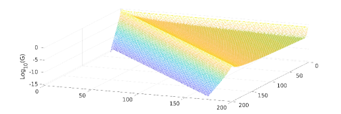
Figure 5: Log-plot of the $200\times 200$ submatrix of the solution $G$ for the coefficients (15).

We have compared our approach (QT-based) with the approximation obtained by truncating $A_{-1}$, $A_{0}$ and $A_{1}$ to finite size, as described in Section 4.2. In Figure 6 we plot the pairs (CPU time, residual errors) for the two different approaches. It is interesting to observe that the method based on truncation cannot reach a sufficiently accurate approximation. For the first problem, the CPU time required by the method based on truncation for reaching the best accuracy 9.0e-12 is about 122 seconds, while the time taken by our approach to reach the same precision is 5.22 seconds for a speed-up of 23.4. Moreover, our method reaches the best accuracy 1.3e-13 in 8.58 seconds. For the second problem the differences are even more evident. The method based on truncation takes 945.3 seconds to reach the accuracy 2.3e-9 while our method takes 5.48 seconds to approximate the solution with the same accuracy. The speed-up in this case is 172.5. Moreover, our method reaches the highest precision of 1.0e-13 in 27.86 seconds. Also in this problem, all the residuals are measured as $\lVert A_{-1}+A_{0}G+A_{1}G^{2}-G\rVert_{\infty}$.

Figure 6: A QBD example where $G\in\mathcal{EQT}$. Time versus accuracy of the QT-based method and of the truncation method relying on the SMCSolver toolbox. On the left, the QBD defined by coefficients (15); on the right, the case defined by (16).

5 Conclusions

We have introduced a computational framework for handling classes of structured semi-infinite matrices encountered in the analysis of random walks in the quarter plane which include rare events as reset and catastrophes. This framework consists of two matrix classes $\mathcal{QT}_{\infty}^{d}$ and $\mathcal{EQT}$ which extend the quasi Toeplitz matrices introduced in [5] and [6]. We proved that both classes are Banach algebras, that matrices in these classes can be approximated to any arbitrary precision in the infinite norm with a finite number of parameters and that a finite arithmetic can be designed and implemented by extending the cqt-toolbox of [7]. In particular the computation of the invariant probability measure, performed by means of the matrix analytic approach of [35] can be achieved by solving a quadratic matrix equation with coefficients in the classes $\mathcal{QT}_{\infty}^{d}$ or $\mathcal{EQT}$. We have given conditions on the probabilities of the random walk under which the minimal nonnegative solution $G$ of such quadratic matrix equations belongs either to $\mathcal{QT}_{\infty}^{d}$ or to $\mathcal{EQT}$. Examples of algorithms for computing $G$ are given. Numerical experiments, applied to significant problems, show the effectiveness of our approach.

Some issues are still left to investigate. Namely, the analysis of the more general case where the coefficients $A_{i}=T(a_{i})+E_{i}$ have a banded structure, that is $a_{i}(z)$ is a general Laurent polynomial; the study of the specific features of the solution $G$ when $a_{-1}(1)=a_{1}(1)$; and the challenging case of multidimensional random walks with more than two coordinates where the matrix coefficients $A_{i}$ have a multilevel structure.

References

- [1] A. S. Alfa. Applied discrete-time queues. Springer, New York, second edition, 2016.
- [2] K. Avrachenkov, A. Piunovskiy, and Y. Zhang. Hitting times in Markov chains with restart and their application to network centrality. Methodology and Computing in Applied Probability, pages 1–16, 2015.
- [3] D. A. Bini, G. Latouche, and B. Meini. Numerical methods for structured Markov chains. Numerical Mathematics and Scientific Computation. Oxford University Press, New York, 2005. Oxford Science Publications.
- [4] D. A. Bini, S. Massei, and B. Meini. On functions of quasi-Toeplitz matrices. Sbornik: Mathematics, 208(11):1628, 2017.
- [5] D. A. Bini, S. Massei, and B. Meini. Semi-infinite quasi-Toeplitz matrices with applications to QBD stochastic processes. Math. Comp., 87(314):2811–2830, 2018.
- [6] D. A. Bini, S. Massei, B. Meini, and L. Robol. On quadratic matrix equations with infinite size coefficients encountered in QBD stochastic processes. Numer. Linear Algebra Appl., 25(6):e2128, 12, 2018.
- [7] D. A. Bini, S. Massei, and L. Robol. Quasi-Toeplitz matrix arithmetic: a MATLAB toolbox. Numer. Algorithms, 81(2):741–769, 2019.
- [8] D. A. Bini and B. Meini. On the exponential of semi-infinite quasi-Toeplitz matrices. Numer. Math., 141(2):319–351, 2019.
- [9] D. A. Bini, B. Meini, and J. Meng. Solving quadratic matrix equations arising in random walks in the quarter plane. SIAM J. Matrix Anal. Appl (to appear), 2019. arXiv preprint arXiv:1907.09796.
- [10] D. A. Bini, B. Meini, S. Steffé, and B. Van Houdt. Structured Markov Chains Solver: Algorithms. In Proceeding from the 2006 Workshop on Tools for Solving Structured Markov Chains, SMCtools ’06, New York, NY, USA, 2006. ACM.
- [11] A. Böttcher and S. M. Grudsky. Spectral properties of banded Toeplitz matrices. SIAM, 2005.
- [12] O. Bénichou, M. Coppey, M. Moreau, P.-H. Suet, and R. Voituriez. Optimal search strategies for hidden targets. Physical Review Letters, 94(19), 2005.
- [13] Y. Chen, R. Boucherie, and J. Goseling. Necessary conditions for the compensation approach for a random walk in the quarter-plane. Queueing Systems, 2019.
- [14] P. du Bois-Reymond. Ueber die fourierschen reihen. Nachrichten von der Königl. Gesellschaft der Wissenschaften und der Georg-Augusts-Universität zu Göttingen, 1873:571–584, 1873.
- [15] M. R. Evans and S. N. Majumdar. Diffusion with stochastic resetting. Physical Review Letters, 106(16), 2011.
- [16] G. Fayolle, R. Iasnogorodski, and V. Malyshev. Random Walks in the Quarter-Plane. Springer, 1999.
- [17] L. Flatto and S. Hahn. Two parallel queues created by arrivals with two demands I. SIAM Journal on Applied Mathematics, 44(5):1041–1053, 1984.
- [18] J. Goseling, R. Boucherie, and J.-K. Van Ommeren. A linear programming approach to error bounds for random walks in the quarter-plane. Kybernetika, 52(5):757–784, 2016.
- [19] L. Haque, Y. Q. Zhao, and L. Liu. Sufficient conditions for a geometric tail in a QBD process with many countable levels and phases. Stoch. Models, 21(1):77–99, 2005.
- [20] Q.-M. He. Fundamentals of matrix-analytic methods. Springer, New York, 2014.
- [21] P. Henrici. Applied and computational complex analysis. Vol. 1. Wiley Classics Library. John Wiley & Sons, Inc., New York, 1988. Power series—integration—conformal mapping—location of zeros, Reprint of the 1974 original, A Wiley-Interscience Publication.
- [22] A. Horváth and M. Gribaudo. Matrix geometric solution of fluid stochastic Petri nets. In Matrix-analytic methods (Adelaide, 2002), pages 163–182. World Sci. Publ., River Edge, NJ, 2002.
- [23] S. Janson and Y. Peres. Hitting times for random walks with restarts. SIAM Journal on Discrete Mathematics, 26(2):537–547, 2012.
- [24] G. Latouche, S. Mahmoodi, and P. G. Taylor. Level-phase independent stationary distributions for M/1-type Markov chains with infinitely-many phases. Perform. Eval., 70(9):551–563, Sept. 2013.
- [25] G. Latouche and V. Ramaswami. Introduction to matrix analytic methods in stochastic modeling. ASA-SIAM Series on Statistics and Applied Probability. Society for Industrial and Applied Mathematics (SIAM), Philadelphia, PA; American Statistical Association, Alexandria, VA, 1999.
- [26] G. Latouche and P. Taylor. Truncation and augmentation of level-independent QBD processes. Stochastic Process. Appl., 99(1):53–80, 2002.
- [27] M. A. Lomholt, K. Tal, R. Metzler, and K. Joseph. Lévy strategies in intermittent search processes are advantageous. Proceedings of the National Academy of Sciences, 2008.
- [28] S. C. Manrubia and D. H. Zanette. Stochastic multiplicative processes with reset events. Physical Review E, 59(5):4945, 1999.
- [29] R. E. Megginson. An introduction to Banach space theory, volume 183 of Graduate Texts in Mathematics. Springer-Verlag, New York, 1998.
- [30] M. Miyazawa. Tail decay rates in double QBD processes and related reflected random walks. Math. Oper. Res., 34(3):547–575, 2009.
- [31] M. Miyazawa. Light tail asymptotics in multidimensional reflecting processes for queueing networks. Top, 19(2):233–299, 2011.
- [32] M. Montero and J. Villarroel. Monotonic continuous-time random walks with drift and stochastic reset events. Physical Review E, 87(1):012116, 2013.
- [33] M. Montero and J. Villarroel. Directed random walk with random restarts: The sisyphus random walk. Physical Review E, 94(3):032132, 2016.
- [34] A. J. Motyer and P. G. Taylor. Decay rates for quasi-birth-and-death processes with countably many phases and tridiagonal block generators. Adv. in Appl. Probab., 38(2):522–544, 2006.
- [35] M. F. Neuts. Matrix-geometric solutions in stochastic models. Dover Publications, Inc., New York, 1994. An algorithmic approach, Corrected reprint of the 1981 original.
- [36] T. Ozawa. Stability condition of a two-dimensional qbd process and its application to estimation of efficiency for two-queue models. Perf. Eval., 130:101–118, 2019.
- [37] T. Ozawa and M. Kobayashi. Exact asymptotic formulae of the stationary distribution of a discrete-time two-dimensional QBD process. Queueing Syst., 90(3-4):351–403, 2018.
- [38] L. Robol. Rational Krylov and ADI iteration for infinite size quasi-Toeplitz matrix equations. arXiv preprint arXiv:1907.02753, 2019.
- [39] D. Stanford, W. Horn, and G. Latouche. Tri-layered QBD processes with boundary assistance for service resources. Stoch. Models, 22(3):361–382, 2006.
- [40] B. Van Houdt and C. Blondia. Approximated transient queue length and waiting time distributions via steady state analysis. Stoch. Models, 21(2-3):725–744, 2005.
- [41] B. Van Houdt and C. Blondia. QBDs with marked time epochs: A framework for transient performance measures. In QEST 2005 - Proceedings Second International Conference on the Quantitative Evaluation of SysTems, volume 2005, pages 210–219, 2005.
- [42] J. Van Velthoven, B. Van Houdt, and C. Blondia. Simultaneous transient analysis of QBD Markov chains for all initial configurations using a level based recursion. In Proceedings - 4th International Conference on the Quantitative Evaluation of Systems, QEST 2007, pages 79–88, 2007.
- [43] H. Zhang, D. Shi, and Z. Hou. Explicit solution for queue length distribution of M/T-SPH/1 queue. Asia-Pac. J. Oper. Res., 31(1):1450001, 19, 2014.