Extension of the standard Heisenberg Hamiltonian to multispin exchange interactions

Abstract

An extension of the Heisenberg Hamiltonian is discussed, that allows to go beyond the standard bilinear spin Hamiltonian taking into account various contributions due to multispin interactions having both chiral and non-chiral character. The parameters of the extended Hamiltonian are calculated from first principles within the framework of the multiple scattering Green function formalism giving access to an explicit representation of these parameters in real space. The discussions are focused on the chiral interactions, i.e. biquadratic and three-spin Dzyaloshinskii-Moriya like vector interactions $\vec{\cal{D}}_{ijij}$ (BDMI) and $\vec{\cal{D}}_{ijkj}$ (TDMI), respectively, as well as the three-spin chiral interaction (TCI) $J_{ijk}$. Although all parameters are driven by spin-orbit coupling (SOC), some differences in their properties are demonstrated by calculations for real materials. In particular it is shown that the three-spin chiral interactions $J_{ijk}$ may be topology as well as SOC induced, while the TDMI is associated only with the SOC. As the magnitude of the chiral interactions can be quite sizable, they can lead to a stabilization of a noncollinear magnetic texture in some materials that is absent when these interactions are neglected.

I Introduction

The Heisenberg spin Hamiltonian is nowadays a rather popular tool providing a bridge between the electronic structure of magnetic materials and their spin-dynamical and finite-temperature magnetic properties. However, restriction of the classical model to only isotropic bilinear exchange parameters is not always able to describe successfully the experimental findings. In this case an extension of Heisenberg model is used to take into account specific features of the system under consideration. This concerns in particular the impact of spin-orbit coupling (SOC) leading to magnetocrystalline anisotropy (MCA) and to the spin-space anisotropy of the exchange coupling described by an exchange tensor $\underline{J}_{ij}$ instead of scalar parameters. The latter can be reduced to the isotropic exchange parameters $J_{ij}$ and chiral Dzyaloshinskii-Moriya (DM) vector $\vec{D}_{ij}$ representing the antisymmetric part of the exchange tensor ${\underline{J}}_{ij}$.

Still, this form of the Hamiltonian implies for example neglecting the dependence of the exchange parameters on the relative orientation of the magnetic moments in the system. To go beyond this bilinear approximation for the inter-atomic exchange interactions, one can take into account higher-order contributions to the Heisenberg Hamiltonian, i.e., biquadratic, fourth-order three-spin, four-spin interactions, etc. terms Harris and Owen (1963); Huang and Orbach (1964); Allan and Betts (1967); Iwashita and Uryû (1974); Iwashita and Uryû (1976); Aksamit (1980); Brown (1984); Ivanov et al. (2014); Antal et al. (2008).

The origin of higher-order interactions was discussed already many years ago by various authors Kittel (1960); Tanaka and Uryû (1977); MacDonald et al. (1988), focusing on those being isotropic in spin space. Obviously, the dominating mechanism responsible for these terms can be different for different materials. Kittel Kittel (1960) discussing the transition from the antiferromagnetic (AFM) to the ferromagnetic (FM) state in metamagnetic materials (including metals) suggested an important role of the biquadratic exchange interaction due to exchange magnetostriction caused by a dependence of the exchange interaction on the volume during an AFM/FM transition. MacDonald et al. MacDonald et al. (1988) discussed the Hubbard model Hamiltonian, which can be transformed in the limit of large on-site Coulomb interaction $U$ and assuming half-filling of the electron energy bands implying electron localization around atomic sites to a form equivalent to the Heisenberg spin Hamiltonian. An expansion of the Hamiltonian in powers of the ratio $t/U$ gives access to high-order terms of the spin Hamiltonian with bilinear and four-spin exchange interactions $\sim t^{2}/U$ and $\sim t^{4}/U^{3}$, respectively MacDonald et al. (1988); Bulaevskii et al. (2008); Batista et al. (2016). In the absence of a magnetic field braking time reversal symmetry of the system the three-spin term should vanish as it is antisymmetric with respect to time reversal transformation. Tanaka and Uryu Tanaka and Uryû (1977) have derived the four-spin interactions based on the Heitler-London theory by expanding the ground state energy in terms of the overlap integrals between the orbitals of electrons located at different lattice sites. Detailed calculations of bilinear and biquadratic exchange interactions within a real-space tight-binding framework have been performed for FM Fe by Spisak and Hafner Spišák and Hafner (1997) who demonstrate a significant contribution of the biquadratic exchange interactions to the Curie temperature.

During the last decade the interest in skyrmions grew rapidly because their specific magnetic texture stabilized by chiral spin interactions makes them attractive for various spintronic applications (see e.g. Moreau-Luchaire et al. (2016); Karube et al. (2016); Dupé et al. (2016)). Most investigations in the field were restricted to the bilinear Dzyaloshinskii-Moriya interaction (DMI) and focused on materials for which a strong DMI can be expected Simon et al. (2014); Polesya et al. (2014); Dupé et al. (2016).

The DMI is caused by spin-orbit coupling (SOC) and is non-zero in non-centrosymmetric systems only. Competing with isotropic FM or AFM interactions it leads to a deviation from the collinear magnetic state by creating a helimagnetic structure in the absence of an external magnetic field, characterized by a non-zero vector spin chirality $\vec{\chi}_{ij}=\hat{s}_{i}\times\hat{s}_{j}$ .

Recently, first-principles investigations have been performed going beyond the bilinear approximation, taking into account higher-order chiral interactions Brinker et al. (2019); Lászlóffy et al. (2019) in the extended Heisenberg model. The calculation of the chiral biquadratic DMI-like interaction (BDMI) for deposited dimers Brinker et al. (2019) has demonstrated that its magnitude can be comparable to that of the conventional bilinear Dzyaloshinskii-Moriya interaction, implying the non-negligible role of biquadratic contributions. In addition, the first-principles investigations on the magnetic properties of Fe monatomic chains on a Re(0001) substrate have shown Lászlóffy et al. (2019) that chiral four-spin interactions can be responsible for the opposite chirality of the spin spirals when compared to that determined by DMI.

Another type of chiral interaction, the three-spin chiral interaction (TCI) term, was discussed as a possible source for the formation of chiral magnetic phases Parihari and Pati (2004); Bauer et al. (2014). This three-spin interaction term in the Heisenberg Hamiltonian, $\sum_{i,j,k}J_{ijk}\hat{s}_{i}\cdot(\hat{s}_{j}\times\hat{s}_{k})$, gives a non-zero contribution only for a non-coplanar magnetic structure, i.e. in the case of non-zero scalar chirality, defined as a counter-clock-wise triple scalar product $\chi_{ijk}=\hat{s}_{k}\cdot(\hat{s}_{i}\times\hat{s}_{j})$. This can lead to the transition to a chiral spin liquid state, for which the time-reversal symmetry is broken spontaneously by the appearance of long-range order of scalar chirality even in the absence of long-range magnetic order or an external magnetic field Wen et al. (1989); Rokhsar (1990); Freericks et al. (1991); Sen and Chitra (1995). Describing a transition in a frustrated quantum spin system from a spin liquid to a chiral spin liquid state within the framework of the Hubbard model, it was shown that expanding the Hubbard Hamiltonian in powers of $t/U$ leads to a third-order term which is proportional to the flux $\Phi_{ijk}$ enclosed by the three-spin loop Kostyrko and Bułka (2011); Lecheminant and Tsvelik (2017), giving rise to the three-spin interaction Kostyrko and Bułka (2011); Lecheminant and Tsvelik (2017) entering the spin Hamiltonian represented by $J_{ijk}=(24/U^{2})|t_{ij}||t_{jk}||t_{ki}|\sin(\Phi_{ijk}/\Phi_{0})$ (with $\Phi_{0}=\hbar c/e$) Rokhsar (1990); Sen and Chitra (1995); Scarola et al. (2004); Bauer et al. (2014). Note that the phase $\Phi_{ijk}/\Phi_{0}$ is generated by the external magnetic field breaking time-reversal symmetry in the system. In the presence of an inhomogeneous magnetic texture in the system, the finite geometric quantum phase of the electron wave function can appear due to the $s-d$-interaction, which can be described in terms of the emergent effective electromagnetic potential leading to an effective magnetic field $B^{eff}\sim\chi_{ijk}$Fujita et al. (2011); Takashima and Fujimoto (2014) giving rise to the three-spin energy contribution $\sim\chi_{ijk}^{2}$, that can be associated with the topology-induced three-spin chiral-chiral exchange interaction Grytsiuk et al. (2020). These interactions have been introduced and evaluated on the basis of first-principles electronic structure calculations for the B20-type compounds MnGe and FeGe. The authors report also about another type of three-spin interaction having topological origin, so called spin-chiral interactions, which are however non-zero only if spin-orbit interaction is taken into account.

Discussing skyrmion-hosting materials, the formation of skyrmion magnetic texture is usually ascribed to the DMI, implying the lack of the inversion symmetry in these systems. However, recently it was suggested that the magnetic frustration could stabilize skyrmions even in materials with centrosymmetric lattices. This idea was proposed and discussed by various authors within theoretical investigations Okubo et al. (2012); Batista et al. (2016); Hayami et al. (2017). In these works complex superstructures or the skyrmion-lattice state are characterized by multiple ordering wave vectors (multiple-Q), allowing to characterize a non-coplanar magnetic structure via a double-Q description. This approach applied to metallic systems allowed to demonstrate that the non-coplanar vortex state can be stabilized having lower energy than the helimagnetic structure expected due to RKKY interactions Solenov et al. (2012). Solenov et al. Solenov et al. (2012) showed that such a non-coplanar state can be stabilized even in the absence of SOC, i.e. without the DMI. The authors attribute this feature of a double-Q state to the chirality-induced emergent magnetic field associated with a persistent electric current in such systems (see e.g. Bruno and Dugaev (2005); Lux et al. (2018); Tatara (2018)), which is proportional to the scalar chirality in the system. In terms of the extended spin Hamiltonian, the above mentioned property can be attributed to the three-spin interaction term also proportional to the scalar chirality in the system.

In this contribution we present a coherent computational scheme that allows to calculate the parameters of the extended Heisenberg Hamiltonian to any order. The impact of higher order terms going beyond the bilinear level and their anisotropy is discussed on the basis of corresponding numerical results for various systems.

II Electronic structure

Following our previous work Mankovsky et al. (2019), we consider the change of the grand canonical potential caused by the formation of a modulated spin structure seen as a perturbation. This quantity is represented in terms of the Green function $G_{0}(E)$ for the FM reference state and its modification due to the perturbation. Neglecting all temperature effects, and denoting the corresponding change in the Green function $\Delta G(E)$ one can write for the change in energy:

$$\Delta{\cal E} \approx -\frac{1}{\pi}\mbox{Im}\,\mbox{Tr}\int^{E_{F}}dE\,(E-E_{F})\,\Delta G(E)\;,$$ (1)

with the expansion

$$\Delta G(E) = G_{0}\Delta VG_{0}$$ (2)

$$+G_{0}\Delta VG_{0}\Delta VG_{0}$$

$$+G_{0}\Delta VG_{0}\Delta VG_{0}\Delta VG_{0}$$

$$+G_{0}\Delta VG_{0}\Delta VG_{0}\Delta VG_{0}\Delta VG_{0}+...\;,$$

for $\Delta G(E)$, where $\Delta V$ is the perturbation operator associated with the modulated spin structure. For the sake of readability we dropped the energy argument for the unperturbed Green function $G_{0}(E)$.

Using the FM state as a reference state, the perturbation connected with the tilting of rigid magnetic moments on lattice sites $i$ has the real space representation Mankovsky and Ebert (2017); Mankovsky et al. (2019)

$$\Delta V(\vec{r}) = \sum_{i}\beta\big{(}\vec{\sigma}\cdot\hat{s}_{i}-\sigma_{z}\big{)}B_{xc}(\vec{r})\;,$$ (3)

where ${\vec{B}}_{xc}(\vec{r})$ is the spin-dependent part of the exchange-correlation potential, $\vec{\sigma}$ is the vector of $4\times 4$ Pauli matrices and $\beta$ is one of the standard Dirac matrices Rose (1961); Ebert et al. (2016). It is assumed here that ${\vec{B}}_{xc}(\vec{r})$ on site $i$ is aligned along the orientation of the spin moment $\hat{s}_{i}$, i.e.  $\vec{B}_{xc}(\vec{r})={B}_{xc}(\vec{r})\hat{s}_{i}$.

A very convenient and flexible way to represent the electronic Green function $G_{0}(E)$ in Eqs. (1)-(2) is provided by the so-called KKR (Korringa-Kohn-Rostoker) or multiple-scattering formalism. Adopting this approach a real space expression for $G_{0}(\vec{r},\vec{r}\,^{\prime},E)$ can be written in a fully relativistic way as Ebert et al. (2016):

$$G_{0}(\vec{r},\vec{r}\,^{\prime},E) = \sum_{\Lambda_{1}\Lambda_{2}}Z^{n}_{\Lambda_{1}}(\vec{r},E){\tau}^{nn^{\prime}}_{\Lambda_{1}\Lambda_{2}}(E)Z^{n^{\prime}\times}_{\Lambda_{2}}(\vec{r}\,^{\prime},E)$$ (4)

$$-\sum_{\Lambda_{1}}\Big{[}Z^{n}_{\Lambda_{1}}(\vec{r},E)J^{n\times}_{\Lambda_{1}}(\vec{r}\,^{\prime},E)\Theta(r^{\prime}-r)$$

$$\qquad\quad+J^{n}_{\Lambda_{1}}(\vec{r},E)Z^{n\times}_{\Lambda_{1}}(\vec{r}\,^{\prime},E)\Theta(r-r^{\prime})\Big{]}\delta_{nn^{\prime}}\;.$$

Here $Z^{n}_{\Lambda_{1}}(\vec{r},E)$ and $J^{n}_{\Lambda_{1}}(\vec{r},E)$ are the regular and irregular solutions of the single site Dirac equation and ${\underline{\tau}}^{nn^{\prime}}$ is the so-called scattering path operator matrix Ebert et al. (2016). Substituting the expression in Eq. (4) into Eq. (2) and using Eq. (1) one obtains in a straight and natural way a real space expression for the energy change $\Delta\cal E$, which will be used below to derive expressions for the exchange coupling parameters entering the extended Heisenberg Hamiltonian.

The dependence of the energy on the magnetic configuration calculated from first principles via Eqs. (1) to (3) will be mapped onto the extended Heisenberg Hamiltonian

$$H = -\sum_{i,j}J^{s}_{ij}(\hat{s}_{i}\cdot\hat{s}_{j})-\sum_{i,j}\vec{{D}}_{ij}\cdot(\hat{s}_{i}\times\hat{s}_{j})$$ (5)

$$-\frac{1}{3!}\sum_{i,j,k}^{N}J_{ijk}\hat{s}_{i}\cdot(\hat{s}_{j}\times\hat{s}_{k})\;,$$

$$-\frac{2}{p!}\sum_{i,j,k,l}J^{s}_{ijkl}(\hat{s}_{i}\cdot\hat{s}_{j})(\hat{s}_{k}\cdot\hat{s}_{l})$$

$$-\frac{2}{p!}\sum_{i,j,k,l}\vec{{\cal D}}_{ijkl}\cdot(\hat{s}_{i}\times\hat{s}_{j})(\hat{s}_{k}\cdot\hat{s}_{l})\;.$$

Here the prefactors of the various sums account for multiple counting contributions occurring upon summation over all lattice sites, where $p$ specifies the number of interacting atoms; i.e. $p=2$, $p=3$ and $p=4$ correspond to the biquadratic, three-spin and four-spin interactions, respectively. The prefactor $\frac{2}{p!}$ occurs due to the chosen normalization of the exchange parameters, that leads to the same prefactor for the biquadratic term in the Hamiltonian as in the case of the bilinear term. Note that we follow the more common convention Liechtenstein et al. (1984) for the bilinear exchange interaction parameters, while also other conventions are used in the literature Udvardi et al. (2003), as was pointed out previously Polesya et al. (2014). However, it should be stressed that for the sake of simplicity working out the expressions for the exchange parameters in the following, the prefactors are not taken into account, as they appear coherently for the model as well as for the first-principles representations of the energy and cancel each other in the final expression for the exchange parameters.

III Four-spin exchange interactions

Extending the spin Hamiltonian to go beyond the classical Heisenberg model, we discuss first the four-spin exchange interaction terms $J_{ijkl}$ and $\vec{\cal D}_{ijkl}$. The isotropic exchange as well as the z-component of the DMI-like four-spin interactions can be given in terms of the fourth-rank tensor $J^{\alpha\beta\gamma\delta}_{ijkl}$ which accounts also for pair ($k=i,\,l=j$, so-called biquadratic) and three-spin ($l=j$) interactions. The tensor elements $J^{\alpha\beta\gamma\delta}_{ijkl}$ can be calculated using the fourth-order term of the Green function expansion in Eq. (2). Substituting this expression into Eq. (1) and using the sum rule $\frac{dG}{dE}=-GG$ for the Green function, one obtains after integration by parts the forth-order term of the total energy change $\Delta{\cal E}^{(4)}$ given by:

$$\Delta{\cal E}^{(4)} = -\frac{1}{\pi}\mbox{Im}\,\mbox{Tr}\int^{E_{F}}dE\,$$ (6)

$$\times\Delta VG_{0}\Delta VG_{0}\Delta VG_{0}\Delta VG_{0}\;.$$

Using the ferromagnetic state with $\vec{M}||\hat{z}$ as a reference state, and considering the spin-spiral $\vec{s}_{i}=(\sin\theta\cos(\vec{q}\cdot\vec{R}_{i}),\sin\theta\sin(\vec{q}\cdot\vec{R}_{i}),\cos\theta)$ as the source for the perturbation $\Delta V$ at small $\vec{q}$ values, only the $x$ and $y$ components of the exchange tensor get involved (see also Ref. Mankovsky et al. (2019)). Following the scheme used to derive an expression for the bilinear exchange interactions Mankovsky et al. (2019), the fourth-order derivative with respect to the $\vec{q}$-vector gives the elements of the exchange tensor represented via the expression (see Appendix B)

$$J^{\alpha\beta\gamma\delta}_{ijkl} = \frac{1}{2\pi}\mbox{Im}\,\mbox{Tr}\int^{E_{F}}dE\,$$ (7)

$$\Big{[}\underline{T}^{i,\alpha}(E)\,\underline{\tau}^{ij}(E)\underline{T}^{j,\beta}(E)\,\underline{\tau}^{jk}(E)$$

$$\times\underline{T}^{k,\gamma}(E)\,\underline{\tau}^{kl}(E)\underline{T}^{l,\delta}(E)\,\underline{\tau}^{li}(E)\Big{]}\;,$$

where the matrix elements of the torque operator $T^{i,\alpha}_{\Lambda\Lambda^{\prime}}$ are defined as follows:Ebert and Mankovsky (2009)

$$T^{i,\alpha}_{\Lambda\Lambda^{\prime}} = \int_{\Omega_{i}}d^{3}r\,Z^{i\times}_{\Lambda}(\vec{r},E)\,\Big{[}\beta\sigma_{\alpha}B_{xc}^{i}(\vec{r})\Big{]}\,Z^{i}_{\Lambda^{\prime}}(\vec{r},E)\;.$$ (8)

III.1 Non-chiral exchange interactions

The four-spin scalar interaction, and as special cases, also the fourth-order three-spin term with $l=j$, and the biquadratic exchange interaction term with $k=i$ and $l=j$, can also be written in a form often used in the literature, i.e. they can be represented in terms of scalar products of spin directions:

$$H^{(4)}_{s} = -\sum_{i,j,k,l}J^{s}_{ijkl}(\hat{s}_{i}\cdot\hat{s}_{j})(\hat{s}_{k}\cdot\hat{s}_{l})\;.$$ (9)

The parameters $J^{s}_{ijkl}$ (where $s$ means ’symmetric’) are represented by the symmetric part of the exchange tensor of 4-th rank in Eq. (12) and are given by the expression (see Appendix B)

$$J^{s}_{ijkl} = \frac{1}{4}(J_{ijkl}^{xxxx}+J_{ijkl}^{yyyy}+J_{ijkl}^{xxyy}+J_{ijkl}^{yyxx})\;.$$ (10)

The expression for a three-spin or a biquadratic configuration should have a form which can be seen as being composed of two closed loops, e.g.

$$J^{\alpha\beta\gamma\delta}_{ijil} = \frac{1}{2\pi}\mbox{Im}\,\mbox{Tr}\int^{E_{F}}dE\,$$ (11)

$$\Big{(}\underline{T}^{i,\alpha}(E)\,\underline{\tau}^{ij}(E)\underline{T}^{j,\beta}(E)\,\underline{\tau}^{ji}(E)\Big{)}$$

$$\times\Big{(}\underline{T}^{i,\gamma}(E)\,\underline{\tau}^{il}(E)\underline{T}^{l,\delta}(E)\,\underline{\tau}^{li}(E)\Big{)}\;,$$

such that each can be associated with the pair interaction of atoms $i-j$ and $i-l$ and has a form similar to the one appearing in the case of bilinear interactions. This form has a momentum representation determined by the expression $(\underline{\tau}_{\vec{k}}\,\underline{\tau}_{\vec{k}\pm\vec{q}})\,(\underline{\tau}_{\vec{k}^{\prime}}\,\underline{\tau}_{\vec{k}^{\prime}\pm\vec{q}})$, with $\underline{\tau}_{\vec{k}}$ standing for the $\vec{k}$-dependent scattering path matrices, which should ensure the $q^{2}$ dependence of each expression associated with the scalar product of spin moments. This form of the expression implies also that only the site-off-diagonal terms of Green function are involved in its calculation.

Considering in addition the case $l=j$ one arrives at an expression for the biquadratic interactions

$$J^{\alpha\beta\gamma\delta}_{ijij} = \frac{1}{2\pi}\mbox{Im}\,\mbox{Tr}\int^{E_{F}}dE\,$$ (12)

$$\Big{(}\underline{T}^{i,\alpha}(E)\,\underline{\tau}^{ij}(E)\underline{T}^{j,\beta}(E)\,\underline{\tau}^{ji}(E)\Big{)}$$

$$\times\Big{(}\underline{T}^{i,\gamma}(E)\,\underline{\tau}^{ij}(E)\underline{T}^{j,\delta}(E)\,\underline{\tau}^{ji}(E)\Big{)}\;,$$

for which the symmetry with respect to permutation of two spin moments is just a consequence of the invariance of the trace of a product of matrices with respect to cyclic permutation of the matrices. The biquadratic exchange interaction terms (with $k=i$ and $l=j$) can be seen as a linear term of an expansion of the bilinear exchange parameters in powers of $(\hat{s}_{i}\cdot\hat{s}_{j})$, in order to take into account the dependence of these exchange parameters on the relative orientation of the interacting spin magnetic moments on sites $i$ and $j$. Focusing first on the scalar-interaction terms, this leads to the expression

$${H}^{s} = -\sum_{i,j}\tilde{J}_{ij}(\theta_{ij})(\hat{s}_{i}\cdot\hat{s}_{j})$$ (13)

$$= -\sum_{i,j}J_{ij}(\hat{s}_{i}\cdot\hat{s}_{j})-\sum_{i,j}J^{s}_{ijij}(\hat{s}_{i}\cdot\hat{s}_{j})(\hat{s}_{i}\cdot\hat{s}_{j}).$$

Note that both, bilinear and biquadratic terms in Eq. (13) have two contributions from the same pair of atoms, i.e. $i=a,\,j=b$ and $i=b,\,j=a$, with the interactions $J_{ab}=J_{ba}$ and $J_{abab}=J_{baba}$, as it has been mentioned above.

III.2 Chiral multispin DMI-like exchange interactions

Discussing chiral interactions, we start with the exchange interactions represented by the vector characterizing the DMI-like interaction between two spin moments, $i$ and $j$, but taking into account the magnetic configuration of surrounding atoms, leading to the extension of the Heisenberg Hamiltonian written in the following form

$${H}^{a(4)} = \sum_{i,j,k,l}\vec{{\cal D}}_{ijkl}\cdot(\hat{s}_{i}\times\hat{s}_{j})(\hat{s}_{k}\cdot\hat{s}_{l})\;.$$ (14)

Assuming the magnetization direction of the reference system along the $z$ axis, we distinguish between the $x$ and $y$ components of this chiral interaction on the one hand side, and its $z$ component on the other hand as they require different approaches for their calculation. This is in full analogy to the DMI discussed recently Mankovsky and Ebert (2017); Mankovsky et al. (2019).

III.2.1 DMI-like interactions: z-component

The z-component of the four-spin chiral interaction $\vec{{\cal D}}_{ijkl}$, when all site indices $i,j,k,l$ may be different, is represented by the antisymmetric part of the exchange tensor characterizing the interaction between sites $i,j,k$ and $j$. In full analogy to the DMI, ${\cal D}_{ijkj}^{z}$ can be written as follows

$${\cal D}^{z}_{ijkl}=\frac{1}{4}(J^{xyxx}_{ijkl}+J^{xyyy}_{ijkl}-J^{yxxx}_{ijkl}-J^{yxyy}_{ijkl})$$ (15)

with the tensor elements $J^{\alpha\beta\gamma\delta}_{ijkj}$ determined via Eq. (12).

In the following, we will focus on the three-spin DMI-like interactions TDMI (implying $l=j$) and biquadratic vector interactions (with $l=j,k=i$), which were calculated and discussed recently for some systems with special geometry Brinker et al. (2019); Lászlóffy et al. (2019) in comparison with the DMI. Using Eq. (15) for the special case $l=j,k=i$ one has for the $z$ component of the biquadratic interaction the expression (see Appendix B):

$${\cal D}^{z}_{ijij}=\frac{1}{4}(J^{xyxx}_{ijij}+J^{xyyy}_{ijij}-J^{yxxx}_{ijij}-J^{yxyy}_{ijij})\;.$$ (16)

III.2.2 DMI-like interactions: x- and y-compoment

To calculate the $x$ and $y$ components of the four-spin and as a special case the TDMI and BDMI terms in a system magnetized along the $z$ direction, we follow the scheme suggested by the authors for the calculation of the DMI parameters Mankovsky and Ebert (2017); Mankovsky et al. (2019), which exploited the DMI-governed behaviour of the spin-wave dispersion having a finite slope at the $\Gamma$ point of the Brillouin zone. However, in the present case a more general form of perturbation is required, that allows for of the spin moments entering the scalar product in the four-spin energy terms for a tilting towards the $x$ and $y$ axes. For this purpose we assume a 2D spin modulation according to the expression

$$\hat{s}_{i} = (\mbox{sin}(\vec{q}_{1}\cdot\vec{R}_{i})\;\mbox{cos}(\vec{q}_{2}\cdot\vec{R}_{i})\;,\mbox{sin}(\vec{q}_{2}\cdot\vec{R}_{i})\;,$$ (17)

$$\mbox{cos}(\vec{q}_{1}\cdot\vec{R}_{i})\mbox{cos}(\vec{q}_{2}\cdot\vec{R}_{i}))\;,$$

which is characterized by two wave vectors, $\vec{q}_{1}$ and $\vec{q}_{2}$, orthogonal to each other, as for example $\vec{q}_{1}=q_{1}\hat{y}$ and $\vec{q}_{2}=q_{2}\hat{x}$. The microscopic expression for the $x$ and $y$ components of $\vec{\cal D}_{ijkl}$ describing the most general, four-spin interaction, can be obtained on the basis of the third-order term of the Green function expansion in Eq. (2) leading to a corresponding third-order energy contribution

$$\Delta{\cal E}^{(3)} = -\frac{1}{\pi}\mbox{Im}\,\mbox{Tr}\int^{E_{F}}dE(E-E_{F})\,$$ (18)

$$\times G_{0}\Delta VG_{0}\Delta VG_{0}\Delta VG_{0}\;.$$

This is achieved by taking the first derivative with respect to the wave-vectors $\vec{q}_{1(2)}$, the second-order derivative with respect to the wave-vector $\vec{q}_{2}$ and considering finally the limit $q_{1(2)}\to 0$. The components ${\cal D}^{y}_{ijkj}$ and ${\cal D}^{x}_{ijkj}$ are determined this way by the first-order derivative with respect to the wave-vector $\vec{q}_{1}$ and $\vec{q}_{2}$, respectively. The non-zero elements of the first-order derivative in the limit $q_{1(2)}\to 0$ imply an antisymmetric character of the interactions between the magnetic moments on sites $i$ and $j$ in Eq. (14), similar to the case of the conventional DMI. At the same time, the non-zero second-order derivative with respect to $\vec{q}_{2}$ correspond to a scalar interaction between the magnetic moments on sites $k$ and $l$, which is symmetric with respect to a sign change of the wave vector. The same properties should apply to the corresponding contribution to the model spin Hamiltonian in Eq. (14). Equating for the ab-initio and model approaches the corresponding terms proportional to $({\vec{R}}_{i}-{\vec{R}}_{j})_{y}({\vec{R}}_{k}-{\vec{R}}_{l})^{2}_{x}$ and $({\vec{R}}_{i}-{\vec{R}}_{j})_{x}({\vec{R}}_{k}-{\vec{R}}_{l})^{2}_{x}$ (we keep a similar form in both cases for the sake of convenience) gives access to the elements ${\cal D}^{y,x}_{ijkl}$ and ${\cal D}^{y,y}_{ijkl}$, as well as ${\cal D}^{x,x}_{ijkl}$ and ${\cal D}^{x,y}_{ijkl}$, respectively, of the four-spin chiral interaction. As we focus here on TDMI and BDMI, they can be obtained as the special cases $l=j$ and $l=j,k=i$, respectively. With this, the elements of the TDMI vector can be written as follows

$${\cal D}^{\alpha,\beta}_{ijkj} = \epsilon_{\alpha\gamma}\frac{1}{8\pi}\mbox{Im}\,\mbox{Tr}\int^{E_{F}}dE(E-E_{F})\,$$ (19)

$$\Big{[}\underline{O}^{i}\,\underline{\tau}^{ij}\underline{T}^{j,\gamma}\,\underline{\tau}^{jk}\underline{T}^{k,\beta}\,\underline{\tau}^{kj}\underline{T}^{j,\beta}\,\underline{\tau}^{ji}\;$$

$$-\underline{T}^{i,\gamma}\,\underline{\tau}^{ij}\underline{O}^{j}\underline{\tau}^{jk}\underline{T}^{k,\beta}\,\underline{\tau}^{kj}\underline{T}^{j,\beta}\,\underline{\tau}^{ji}\Big{]}\;\,$$

$$+\Big{[}\underline{O}^{i}\,\underline{\tau}^{ij}\underline{T}^{j,\beta}\,\underline{\tau}^{jk}\underline{T}^{k,\beta}\,\underline{\tau}^{kj}\underline{T}^{j,\gamma}\,\underline{\tau}^{ji}\;$$

$$-\underline{T}^{i,\gamma}\,\underline{\tau}^{ij}\underline{T}^{j,\beta}\underline{\tau}^{jk}\underline{T}^{k,\beta}\,\underline{\tau}^{kj}\underline{O}^{j}\,\underline{\tau}^{ji}\Big{]}\;$$

with $\alpha,\beta=x,y$, and $\epsilon_{\alpha\gamma}$ the elements of the transverse Levi-Civita tensor $\underline{\epsilon}=\begin{bmatrix}0&1\\ -1&0\end{bmatrix}$. The matrix elements of the torque operator $T^{i,\alpha}_{\Lambda\Lambda^{\prime}}$ occurring in Eq. (19) are given by Eq. (8), and the overlap integrals $O^{j}_{\Lambda\Lambda^{\prime}}$ are defined in an analogous way Ebert and Mankovsky (2009):

$$O^{j}_{\Lambda\Lambda^{\prime}} = \int_{\Omega_{j}}d^{3}r\,Z^{j\times}_{\Lambda}(\vec{r},E)\,Z^{j}_{\Lambda^{\prime}}(\vec{r},E).$$ (20)

The expression in Eq. (19) gives access to the $x$ and $y$ components of the DMI-like three-spin interactions in Eq. (14)

$${\cal D}^{\alpha}_{ijkj}={\cal D}^{\alpha,x}_{ijkj}+{\cal D}^{\alpha,y}_{ijkj}\;.$$ (21)

An expression for the BDMI also follows directly from Eq. (19) using the restriction $k=i$. This leads to the elements ${\cal D}^{\alpha,\beta}_{ijij}$ determining chiral biquadratic exchange interactions (similar to the case of four-spin interactions), which can be written in the following form

$${\cal D}^{\alpha,\beta}_{ijij} = \epsilon_{\alpha\gamma}\frac{1}{8\pi}\mbox{Im}\,\mbox{Tr}\int^{E_{F}}dE(E-E_{F})\,$$ (22)

$$\Big{[}\Big{(}\underline{O}^{i}\,\underline{\tau}^{ij}\underline{T}^{j,\gamma}\,\underline{\tau}^{ji}\underline{T}^{i,\beta}\,\underline{\tau}^{ij}\underline{T}^{j,\beta}\,\underline{\tau}^{ji}\;$$

$$-\underline{T}^{i,\gamma}\,\underline{\tau}^{ij}\underline{O}^{j}\underline{\tau}^{ji}\underline{T}^{i,\beta}\,\underline{\tau}^{ij}\underline{T}^{j,\beta}\,\underline{\tau}^{ji}\Big{)}$$

$$+\Big{(}\underline{O}^{i}\,\underline{\tau}^{ij}\underline{T}^{j,\beta}\,\underline{\tau}^{ji}\underline{T}^{i,\beta}\,\underline{\tau}^{ij}\underline{T}^{j,\gamma}\,\underline{\tau}^{ji}\;$$

$$-\underline{T}^{i,\gamma}\,\underline{\tau}^{ij}\underline{T}^{j,\beta}\underline{\tau}^{ji}\underline{T}^{i,\beta}\,\underline{\tau}^{ij}\underline{O}^{j}\,\underline{\tau}^{ji}\Big{)}\Big{]}\;.$$

III.3 Chiral exchange: three-spin exchange interactions

Here we discuss the three-spin chiral exchange interaction entering a corresponding extension term to the Heisenberg Hamiltonian

$$H^{(3)} = -\sum_{i\neq j\neq k}^{N}J_{ijk}\hat{s}_{i}\cdot(\hat{s}_{j}\times\hat{s}_{k})\;.$$ (23)

As it follows from this expression, the contribution due to the three-spin interaction is non-zero only in case of a non-co-planar and non-collinear magnetic structure characterized by the triple product $\hat{s}_{i}\cdot(\hat{s}_{j}\times\hat{s}_{k})$ involving the spin moments on three different lattice sites.

Considering the torque acting in a FM system on the magnetic moment of any atom $i$, which is associated with the three-spin interactions, one can evaluate its projection onto an arbitrary direction $\hat{u}$, $T^{\rm(3)}_{ijk,\hat{u}}=-(\partial H^{(3)}/\partial\hat{s}_{i})\cdot(\hat{u}\times\hat{s}_{i})$ , which is equal to $J_{ijk}(\hat{e}_{k}\cdot\hat{u})$. This value is non-zero only in the case of a non-zero scalar product $(\hat{s}_{k}\cdot\hat{u})$, implying that a non-vanishing torque on spin $\hat{s}_{i}$ created by the spin $\hat{s}_{j}$ coupled via the three-spin interaction, requires a tilting of the third spin moment $\hat{e}_{k}$ to have a non-zero projection on the torque direction. In contrast to that, the torque $T^{\rm DM}_{ij,\hat{u}}=\vec{D}_{ij}\cdot\hat{u}$ Mankovsky et al. (2009) acting due to the spin of atom $j$ on the spin moment of atom $i$ via the DMI, is non-vanishing even in the system with all spin moments being collinear. This makes clear that in order to work out the expression for the $J_{ijk}$ interaction term, a more complicated multi-Q modulation Solenov et al. (2012); Okubo et al. (2012); Batista et al. (2016) of the magnetic structure is required when compared to a helimagnetic structure characterized by a wave vector $\vec{q}$, which was used to derive expressions for the $x-$ and $y-$components of the DMI Mankovsky and Ebert (2017); Mankovsky et al. (2019). In addition, similarly to the DMI that gives a non-zero contribution to the energy due to its anti-symmetry with respect to permutation, the energy due to the TCI, for a fixed spin configuration of all three atoms involved, is non-zero only if $J_{ijk}\neq J_{ikj}$, etc. Otherwise, the terms $ijk$ and $ikj$ cancel each other due to the relation $\hat{s}_{i}\cdot(\hat{s}_{j}\times\hat{s}_{k})=-\hat{s}_{i}\cdot(\hat{s}_{k}\times\hat{s}_{j})$.

Thus, to derive an expression for the TCI, we use the 2D non-collinear spin texture described by Eq. (17), which is characterized by two wave vectors oriented along two mutually perpendicular directions, as for example $\vec{q}_{1}=(0,q_{y},0)$ and $\vec{q}_{2}=(q_{x},0,0)$ (for more details see Appendix B).

In this case the spin chirality driven by the three-spin interaction should lead to the asymmetry of the energy $E(\vec{q}_{1},\vec{q}_{2})$ with respect to a sign change of any of the vectors $\vec{q}_{1}$ and $\vec{q}_{2}$, as a consequence of full antisymmetry of the scalar spin chirality. As a result, the three-spin interactions can be derived assuming a non-zero slope of the energy dispersion $E(\vec{q}_{1},\vec{q}_{2})$ as function of the two wave vectors, in the limit $\vec{q}_{1(2)}=0$.

Substituting the spin modulation in Eq. (17) into the spin Hamiltonian in Eq. (23) associated with the three-spin interaction, the second-order derivative of the energy $E^{(3)}(\vec{q}_{1},\vec{q}_{2})$ with respect to $q_{1}$ and $q_{2}$ wave vectors in the limit $q_{1}\to 0$, $q_{2}\to 0$ is given by the expression

$$\frac{\partial^{2}}{\partial\vec{q}_{1}\partial\vec{q}_{2}}E_{H}^{(3)}$$

$$=-\sum_{i\neq j\neq k}J_{ijk}\big{(}\hat{z}\cdot[(\vec{R}_{i}-\vec{R}_{j})\times(\vec{R}_{k}-\vec{R}_{j})]\big{)}\;.$$ (24)

The microscopic energy term of the electron system, giving access to the chiral three-spin interaction in the spin Hamiltonian is determined by the second-order term of the free energy expansion given by the expression

$$\Delta{\cal E}^{(2)} = -\frac{1}{\pi}\mbox{Im}\,\mbox{Tr}\int^{E_{F}}dE(E-E_{F})\,$$ (25)

$$G_{0}\Delta VG_{0}\Delta VG_{0}\;.$$

To make a connection between the two approaches associated with the ab-initio and model spin Hamiltonians, we consider a second-order term with respect to the perturbation $\Delta V$ induced by the spin modulation in Eq. (17). Taking the first-order derivative with respect to $q_{1}$ and $q_{2}$ in the limit $q_{1}\to 0$, $q_{2}\to 0$, and equating the terms proportional to $\big{(}\hat{z}\cdot[(\vec{R}_{i}-\vec{R}_{j})\times(\vec{R}_{k}-\vec{R}_{j})]\big{)}$ with the corresponding terms in the spin Hamiltonian, one obtains the following expression for the three-spin interaction

$$J_{ijk} = \frac{1}{8\pi}\mbox{Im}\,\mbox{Tr}\int^{E_{F}}dE(E-E_{F})\,$$ (26)

$$\Big{[}\underline{T}^{i,x}\,\underline{\tau}^{ij}\underline{T}^{j,y}\,\underline{\tau}^{jk}\underline{O}^{k}\,\underline{\tau}^{ki}-\underline{T}^{i,y}\,\underline{\tau}^{ij}\underline{T}^{j,x}\,\underline{\tau}^{jk}\underline{O}^{k}\,\underline{\tau}^{ki}$$

$$-\underline{T}^{i,x}\,\underline{\tau}^{ij}\underline{O}^{j}\,\underline{\tau}^{jk}\underline{T}^{k,y}\,\underline{\tau}^{ki}\;+\underline{T}^{i,y}\,\underline{\tau}^{ij}\underline{O}^{j}\,\underline{\tau}^{jk}\underline{T}^{k,x}\,\underline{\tau}^{ki}\;$$

$$+\underline{O}^{i}\,\underline{\tau}^{ij}\underline{T}^{i,x}\,\underline{\tau}^{jk}\underline{T}^{k,y}\,\underline{\tau}^{ki}\;-\underline{O}^{j}\,\underline{\tau}^{ij}\underline{T}^{i,y}\,\underline{\tau}^{jk}\underline{T}^{k,x}\,\underline{\tau}^{ki}\Big{]}\;$$

IV Numerical results

In order to illustrate the expressions developed above by their application to realistic systems, corresponding calculations on various representative systems have been performed. Some numerical details of these calculations are described in Appendix A.

IV.1 Four-spin and biquadratic exchange interactions

Figure 1 represents an example for the four-spin exchange parameters $J^{s}_{ijkl}$ calculated on the basis of Eq. (10) for the three $3d$ bulk ferromagnetic systems bcc Fe, hcp Co and fcc Ni. The results are plotted as a function of the distance $R_{ij}+R_{jk}+R_{kl}+R_{li}$, including only the interactions corresponding to $i\neq j\neq k\neq l$, i.e., all sites are different. For these systems the exchange parameters are about two orders of magnitude smaller than the first-neighbor bilinear exchange interactions. However, in general their contribution can be non-negligible due to the large number of such four-spin loops. Therefore, in some particular cases they should be taken into account.

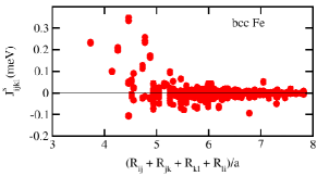
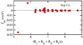
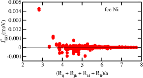
(a)  (b)  (c)

Figure 1: The four-spin interaction exchange parameters $J^{s}_{ijkl}$ according to Eq. (10) calculated for the FM hcp Co (a), bcc Fe (b) and fcc Ni (c) with the magnetization along the $\hat{z}$-axis.

Examples for the scalar biquadratic exchange interaction parameters $J^{s}_{ijij}$ are shown in Fig. 2 for bcc Fe, hcp Co and fcc Ni, and in Fig. 3 for the compounds FePt and FePd having CuAu crystal structure. For comparison, the insets give the corresponding bilinear isotropic exchange interactions. One can see rather strong first-neighbor interactions in bcc Fe and in the compounds FePt and FePd. This confirms the previous theoretical results for bcc Fe Spišák and Hafner (1997), and demonstrates the non-negligible character of biquadratic interactions. This is of course a material-specific property.

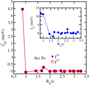
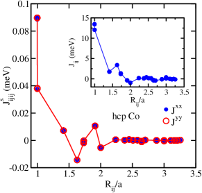
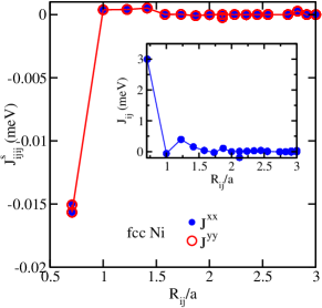
)  (a)  (b)  (c)

Figure 2: Scalar biquadratic exchange interactions in bcc Fe (a), hcp Co (b) and fcc Ni (Ni). The insets show the bilinear exchange interaction parameters calculated for the FM state with the magnetization along the $\hat{z}$-axis.

Figure 3: Scalar biquadratic Fe-Fe exchange interactions in the FM-ordered FePt and FePd with the magnetization along the $\hat{z}$-axis.

IV.2 DMI-like multispin exchange interactions

The properties of the chiral multispin exchange interaction parameters in Eq. (14) can be compared with the DM interactions as both are vector quantities. Similarly to the DMI, these parameters are caused by SOC, i.e. they vanish in the case of SOC = 0. This feature is indeed demonstrated by our test calculations. The calculations have been performed for bulk bcc Fe, for (Pt/$X$/Cu)_n multilayers with $X=$ Mn, Fe and Co, and for an Fe overlayer deposited on TMDC (transition metal dichalcogenide) monolayers, e.g. 1H-TaTe₂ and 1H-WTe₂. The model multilayer system is composed of Pt, $X$ and Cu on subsequent (111) layers of the fcc lattice, without structural relaxation. In the case of the Fe/TMDC systems the structural relaxation has been performed both within the layers as well as in the $z$ direction perpendicular to the layer plane.

The calculations demonstrate similar symmetry properties of the BDMI when compared with the conventional DMI, as was already pointed out recently Brinker et al. (2019). In bcc Fe having inversion symmetry, the BDMI is equal to zero, while it is finite in the multilayer and the Fe/TMDC systems, following the properties of the DMI interactions. Figure 4 gives results for the $z$-component of the chiral biquadratic exchange interactions, ${\cal D}^{z}_{ijij}$, calculated for a Fe overlayer deposited on a TaTe₂ and WTe₂ single layers, respectively, on the basis of Eq. (21). As one can see, ${\cal D}^{z}_{ijij}$ has a significant magnitude when compared to the bilinear DMI parameters. Interestingly, the $x$ and $y$ components in these two materials are much smaller than the corresponding components of the bilinear DMI.

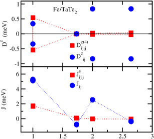
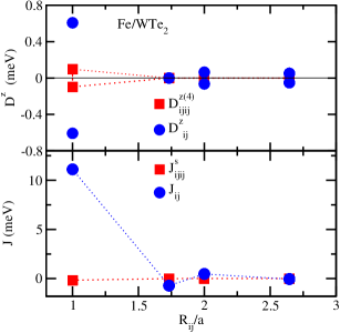
(a)  (b)

Figure 4: $z$-component of the BDMI (squares, top) and biquadratic scalar interactions (squares, bottom) as a function of the site distance $R_{ij}$ (in multiples of the lattice parameter $a$). Results are shown for a Fe overlayer deposited on a single layer of TaTe₂ (a) and WTe₂ (b), in comparison with DMI and bilinear interaction parameters shown by circles.

In the case of the multilayer systems (Pt/Fe/Cu)_n, (Pt/Mn/Cu)_n and (Pt/Co/Cu)_n all three components, $x,y,z$, have the same order of magnitude as it is seen in Fig. 5. The orientation of these interactions between first nearest neighbor sites is shown in Fig. 6. As can be seen from Table 1, in contrast to the Fe/TMDC system, all components are more than one order of magnitude smaller than the corresponding DMI components.

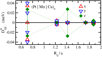
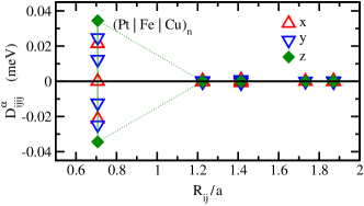
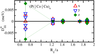
(a)  (b)  (c)

Figure 5: The $x$-, $y$- and $z$-components of chiral biquadratic exchange interaction, $\vec{{\cal D}}_{ijij}$, between the magnetic 3d-metals $X$ in (Pt/$X$/Cu)_n multilayers with $X=$ Mn (a), Fe (b), and Co (c), plotted as a function of the interatomic distance $R_{ij}$. The orientation of the interaction vectors between first nearest neighbors is shown in Fig. 6

Figure 6 shows schematically the in-plane components of the DMI and BDMI, which have the same orientation for (Pt/Fe/Cu)_n and (Pt/Mn/Cu)_n, but not for (Pt/Co/Cu)_n. The $y$-component of ${\cal D}^{y}_{ijij}$ representing the interaction between atoms with $\vec{R}_{ij}=a(0.707,0,0)$ are given in Table 1. These values give the total in-plane interaction as for the taken pair of atoms ${\cal D}^{x}_{ij}=0$ and ${D}^{x}_{ij}=0$. Note also that in (Pt/Mn/Cu)_n the ${\cal D}^{z}_{ijij}$ component has an opposite sign when compared to ${D}^{z}_{ij}$.

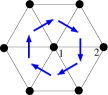
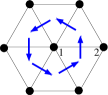
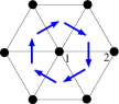
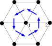
(a)      (b)

Figure 6: Orientation of the DMI vector $\vec{D}_{ij}$ (a) and the vector of the BDMI $\vec{{\cal D}}_{ijij}$ (b) corresponding to the interaction of the first neighbor 3d-atoms $X$ in (Pt/$X$/Cu)_n multilayers: for $X=$ Mn (left), Fe (middle), and Co (right). The magnitude of the interactions are given in Table 1.

	${D}^{y}_{ij}$	${D}^{z}_{ij}$	${\cal D}^{y}_{ijij}$	${\cal D}^{z}_{ijij}$
(Pt/Mn/Cu)n	-1.14	-1.22	-0.039	0.031
(Pt/Fe/Cu)n	0.17	0.35	0.024	0.034
(Pt/Co/Cu)n	0.63	0.40	-0.003	0.008

Table 1: The $y$- and $z$-components of the DMI and chiral biquadratic exchange interaction (in meV) between 3d-metals in (Pt/$X$/Cu)_n multilayers ($X=$ Mn, Fe, Co). The $y$- component corresponds to the interactions between atoms 1 and 2 (see Fig. 6) with $\vec{R}_{12}=a(0.707,0,0)$. For this geometry ${\cal D}^{y}_{1212}$ and ${D}^{y}_{12}$ represent the magnitude of the in-plane projection of corresponding interactions with the first nearest neighbors, as in this case ${\cal D}^{x}_{1212}=0$ and ${D}^{x}_{12}=0$.

Similar to the DMI and BDMI, the TDMI $\vec{\cal D}_{ijkj}$ is a SOC-induced interaction between atoms $i$ and $j$ which depends on the relative orientation of the spin moments of the atoms $j$ and $k$. In contrast to the biquadratic interaction, it does not vanish for centrosymmetric systems, as it is demonstrated by the calculations for bcc Fe represented in Fig. 7. Let us consider the TDMI as the DMI-like interaction between atoms $i$ and $j$ which depends on the relative orientation of the spin moment of the atoms $j$ and $k$. Fig. 7(a) displays the dependence of the components ${\cal D}^{x}_{ijkj}$ and ${\cal D}^{y}_{ijkj}$ of the DMI-like interaction between the first nearest neighbors (distance $|\vec{R}_{ij}|$) in bcc Fe as a function of the position of the third atom $k$. One finds obviously a different sign for the various interactions for the same value of $|\vec{R}_{ij}|+|\vec{R}_{jk}|+|\vec{R}_{ki}|$ implying a dependence of the ${\vec{\cal D}}_{ijkj}$ interaction on the relative position of the third atom (see Fig. 7(b)). In the case of a collinear magnetic structure this property results in a compensation when summing over all surrounding atoms $k$, i.e. $\sum_{k}\vec{\cal D}_{ijkj}=0$, despite the finite magnitude of the individual interactions $|\vec{\cal D}_{ijkj}|\neq 0$ for each triple of atoms. In other words, the TDMI is canceled out in centrosymmetric collinear magnetic systems, giving no contribution to the energy as the DMI and BDMI. In the case of a non-collinear magnetic texture, however, the sum can be non-zero leading to a non-vanishing contribution of the TDMI term to the energy that may stabilize the non-collinear magnetic structure.

To understand this behavior, one can consider once more the DMI between two spin moments $\vec{s}_{i}$ and $\vec{s}_{j}$, caused by SOC seen as a perturbation (see e.g. Brinker et al. (2019)). Within a real space consideration the origin of the DMI can be associated with the SOC of the electrons on a third atom arranged in the vicinity of the atoms $i$ and $j$. Following the work by Brinker et al. Brinker et al. (2019) this will be called the ’SOC carrying’ atom. The anisotropy of the exchange interaction of two spin moments associated with a single ’SOC carrying’ atom in this case is non-zero, while the DMI and its symmetry properties are determined by all surrounding ’SOC carrying’ atoms and by the crystal symmetry. In particular for a centrosymmetric system, this leads to a cancellation when summing all individual contributions. In the case of the TDMI one has to make an explicit summation over the ’third’ atom $k$ involved in the interaction, which can be seen as the ’SOC carrying’ one. As a result, for any triple of atoms in a centrosymmetric system the TDMI is non-zero. For the case of a collinear magnetic structure, however, the summation over all atoms $k$ leads to a canceling of the TDMI. In the case of a non-collinear magnetic structure, on the other hand, this does not have to apply.

Note that these conclusions based on the results obtained for a frame of reference with the $\hat{z}$ axis oriented along the crystallographic [001] direction should hold for any other frame of reference. Nevertheless, it is more convenient to discuss the interactions using a frame of reference with the $z$ axis, as well as the magnetization, oriented along the [111] crystallographic direction, as it is shown in Fig. 7(b). The arrows represent the direction of the TDM interaction in the $(x,y)$ plane between the gray atom $1$ at the center and the red atom $2$ behind, induced by tilting of the moment of the third atom $(3)$ (connected in the picture by dashed lines with the atoms $1$ and $2$). One can see that the direction of this interaction depends on the position of atom $3$.

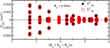
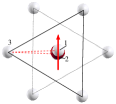
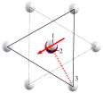
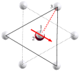
(a)      (b)

Figure 7: (a) TDM interactions for bcc Fe with ’vector’ coupling between the gray atom in the center (atom 1) and the red atom behind (atom 2) with the third atom (atom 3) coupled with atom 2 via scalar coupling. The magnitude of this three-spin interaction energy is 0.004 meV for all three cases shown in the figure.

However, in the case of systems without inversion symmetry, the TDM interactions do not cancel each other and can play a certain role in the formation of the magnetic ground state configuration. This is demonstrated by calculations for (Pt/$X$/Cu)_n multilayer systems. Fig. 8 shows corresponding results for the (Pt/Mn/Cu)_n multilayer system where, using a similar representation as before, the arrows represent the ’vector’ interactions (i.e. $\sim(\hat{s}_{1}\times\hat{s}_{2})$) between atoms $1$ and $2$, controlled by the third atom $3$. Obviously, the direction of this interaction depends on the position of the third atom as one can see in Fig. 8 (a) and (b). Moreover, the magnitude of this interaction follow the 3-fold in-plane symmetry of the system, and is comparable to that of the biquadratic interactions and is smaller by more than one order of magnitude when compared to the DMI interactions.

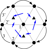
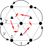
(a)  (b)

Figure 8: The plane-projected three-spin DMI-like interactions (TDMI) between atoms 1 (in the center) and 2 (on the hexagon) in the presence of atom 3 (relative position shown by a bended arrow) in the (Pt/Mn/Cu)_n multilayer. (a) represents the vectors when the third atom follows site 2(2’) on the hexagon in the clock-wise direction and (b) when the third atom follows site 2(2’) in the anti-clock-wise direction. The long vectors represent the interactions with magnitude 0.068 meV, while the short ones correspond to the interactions with 0.032 meV. The z-component of the interactions is -0.006 meV between atoms 1 and 2 (2’) in (a) and 0.006 between atoms 1 and 2 (2’) in (b). The triangles show the position of Pt atoms on the neighboring layer.

IV.3 Chiral exchange: Three-spin exchange interactions

IV.3.1 First-principles calculations

Eq. (26) was used to calculate the three-spin interaction parameters for a couple of representative 3D and 2D systems. Fig. 9 (a) represents the results on the TCI for 1ML bcc Fe(110). The DMI and BDMI for this system vanish due to inversion symmetry. The TCIs calculated without SOC (closed symbols) included for various triangles of different size do not change upon permutation of any two atoms, i.e. $J_{123}=J_{132}$. As discussed above, this leads to a cancellation of the energy contribution due to these two terms. However, switching SOC on breaks the symmetry of the TCI with respect to permutations, implying $J_{123}\neq J_{132}$. Corresponding data are shown in Fig. 9 (a) by open symbols. As a consequence, the contribution due to the TCI to the magnetic energy of the system should in general be finite.

For further discussions it is convenient to introduce reduced TCI parameters defined as $\tilde{J}_{ijk}=J_{ijk}-J_{ikj}$ for counter-clock-wise sequences of atoms $i,j,k$. Corresponding results for $\tilde{J}_{ijk}$ for 1ML Fe(110) are shown in Fig. 9 (b). In this case the energy term $H^{(3)}$ given in Eq. (23) associated with $\tilde{J}_{ijk}$ can be written as follows

$$H^{(3)} = -\sum_{i\neq j\neq k}\tilde{J}_{ijk}\chi_{ijk}$$ (27)

with the scalar spin chirality $\chi_{ijk}$, accounting only the contributions due to the counter-clock-wise sequence of atoms $i,j,k$. As one can see in Fig. 9 (b), the magnitude of the TCI decreases quickly with an increasing perimeter of a triangle. As a consquence one may restrict the sum in Eq. (27) to the two smallest triangles. In this case, making use of the symmetry of $\tilde{J}_{ijk}$ with respect to cyclic permutation, i.e. accounting for $\tilde{J}_{123}=\tilde{J}_{312}=\tilde{J}_{231}=\tilde{J}_{\Delta}$, the expression for $H^{(3)}$ can be further simplified to

$$H^{(3)} = -\tilde{J}_{\Delta 1}\sum_{(i,j,k)\in\Delta 1}\chi_{ijk}-\tilde{J}_{\Delta 2}\sum_{(i,j,k)\in\Delta 2}\chi_{ijk}\;.$$ (28)

The TCI parameters calculated for 1ML Fe(110) can be compared to the TDMI parameters, as both are non-vanishing in centrosymmetric systems. Considering the smallest triangle $\Delta 1$, we have for the TCI $\tilde{J}_{\Delta 1}=0.21$ meV, while the z-component of the TDMI (the only non-vanishing one) between spin moments 1 and 2 is found to be $D^{z}_{1213}=0.0014$ meV and $D^{z}_{1214}=-0.039$ (the positions of the third atoms are shown in Fig. 9) demonstrating that the TDMI is much weaker when compared to the TCI.

On the other hand, the origin of the TCI can be discussed in more detail on the basis of the spin-chiral interaction introduced by Grytsiuk et al. Grytsiuk et al. (2020). According to this approach, the TCI can be associated with a topological orbital moment $\vec{L}^{TO}_{ijk}$ induced on the atoms of each triangle Lux et al. (2018) due to the non-coplanar orientation of the spin magnetic moments. According to Refs. Grytsiuk et al. (2020); Feng et al. (2020); Taguchi et al. (2001), one has $\vec{L}^{TO}_{ijk}=\kappa^{TO}_{ijk}\chi_{ijk}\vec{n}_{ijk}$, where $\kappa^{TO}_{ijk}$ is the topological orbital susceptibility, and $\vec{n}_{ijk}$ is the normal to the triangle $\Delta_{i,j,k}$. Accounting for the SOC, the interaction energy between spin moments on the atoms with corresponding topologically induced orbital moments can be written as $~{}\sim\sum_{i}\xi\vec{L}^{TO}_{i}\cdot\vec{s}_{1}$ where $\xi$ is the spin-orbit interaction parameter for atom $i$ having the spin moment $\vec{s}_{i}$. In the case of all atoms being equivalent, the sum can be written as $~{}\sim\xi\kappa^{TO}_{ijk}\chi_{ijk}(\vec{n}_{ijk}\cdot\langle\vec{s}\rangle)$, with $\langle\vec{s}\rangle=\vec{s}_{i}+\vec{s}_{j}+\vec{s}_{k}$. This expression shows that the dependence of the three-spin interactions on the orientation of spin magnetic moments is given by their projection on the normal vector of a triangle that is proportional to the flux of local spin magnetization through the triangle area.

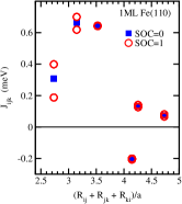
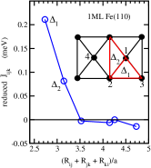
(a)  (b)

Figure 9: (a) Three-spin chiral exchange interaction parameters $J_{ijk}$ calculated for bcc Fe (110) with SOC = 0 (closed squares) and SOC=1 (open circles). (b) The reduced TCI $\tilde{J}_{ijk}$ for bcc Fe (110). Inset in (b) shows two triangles in Fe(110) system, having the smallest size $\Delta 1$ and $\Delta 2$.

The dependence of the TCI on the orientation of the magnetization has been investigated also for 1ML bcc Fe (110). The parameters calculated for the smallest triangle, $\tilde{J}_{\Delta 1}(\theta)$ are plotted in Fig. 10(a) as a function of the angle $\theta$ between the magnetization and the triangle normal. As one can see, the results given by circles are in perfect agreement with the function $\tilde{J}_{\Delta 1}(0)cos\theta$, in line with the discussion above.

An increase in temperature results in general in an increase of magnetic disorder in the system leading to a corresponding decrease of the net magnetization that finally vanishes at the critical temperature $T_{C}$. In order to investigate the dependence of the TCI parameter $\tilde{J}_{ijk}$ on the normalized magnetization seen as the order parameter, calculations have been performed for the partially ordered state described by means of the relativistic disorder local moment (RDLM) approach Gyorffy et al. (1985); Ebert et al. (2015). In these calculations the exchange parameters $\tilde{J}_{ijk}$ are associated with the energy change due to a tilting of the spin magnetic moments of a triple of atoms with respect to the magnetization direction of the reference system, accounting for partial (as well as full) magnetic disorder of all surrounding atoms. Fig. 10(b) represents the results for the smallest triangle, showing a decrease of $\tilde{J}_{\Delta 1}$ by about twice approaching $|\langle\vec{m}\rangle|/m_{0}\approx 0.5$, and staying nearly unchanged for larger disorder i.e. higher temperature. The non-vanishing behavior of the TCI parameters can be understood by keeping in mind their dependence on the local magnetic order.

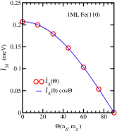
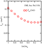
(a)  (b)

Figure 10: Three-spin chiral exchange interaction parameters $\tilde{J}_{\Delta}$ calculated for the smallest triangle $\Delta 1$ in 1 ML of Fe(110): (a) as a function of the orientation of magnetization with respect to normal vector of triangle, and (b) as function of average reduced magnetization $|\langle\vec{m}\rangle|/m_{0}$.

In Fig. 11 one can see in addition a strong dependence of the TCI on the occupation of the valence states, with the magnitude reaching its maximum below the true Fermi energy.

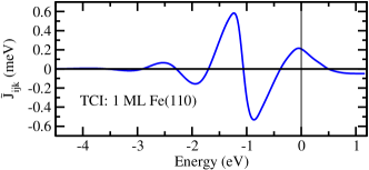
Figure 11: The reduced three-spin chiral interactions $\tilde{J}_{ijk}(E)$ for the smallest triangle $\Delta 1$ in 1 ML of Fe(110) as a function of occupation.

Fig. 12(a) shows the TCI parameters calculated for centrosymmetic bcc Fe, as a function of the perimeter of the considered triangles for three different orientations of the magnetic moment: [001] (circles), [111] (squares) and [110] (diamonds). The results given in Fig. 12(a) (top panel) have been obtained without including the SOC. As one can see, the TCI parameters do not depend on the orientation of the magnetization. However, according to the discussions above, this leads to a cancellation of their contribution to the energy upon summation over all sites in the lattice. In the presence of SOC, on the other hand, the interactions shown in Fig. 12(a) (bottom panel) change their magnitude upon permutation, i.e. $J_{123}\neq J_{132}$. The corresponding dependence on the relative orientation of the magnetization and the triangle normal is also given in Fig. 12(b) for four different triangles, assuming the magnetization oriented along the $z$ axis. In the case of triangles 1 and 3 the TCI parameters $\tilde{J}_{ijk}$ are non-zero. This is not the case for the triangles 2 and 4 as the flux of the magnetization through their area is equal to zero. This changes however due to change of the magnetization toward the [111] and [110] crystallographic directions (see Fig. 12(a), bottom panel).

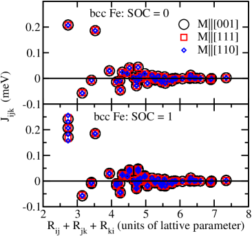
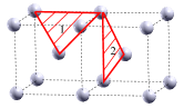
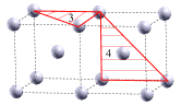
(a)    (b)

Figure 12: (a) Three-spin chiral exchange interaction parameters calculated for bcc Fe without (top panel) and with SOC (bottom panel), respectively, for three different magnetization directions: [001] circles, [111] (squares) and [110] (diamonds). (b) The reduced TCI calculated for the triangles 1,2,3,4, assuming magnetization along z direction: $\tilde{J}^{1}_{\Delta}=0.07$ meV, $\tilde{J}^{2}_{\Delta}=0.0$ meV, $\tilde{J}^{3}_{\Delta}=0.005$ meV, $\tilde{J}^{4}_{\Delta}=0.0$ meV.

Fig. 13 shows the three-spin chiral interaction between 3$d$ atoms in the (Pt/$X$/Cu)_n multilayer system, with $X$ = Mn (a), Fe (c) and Co (e), calculated without (closed squares) and with SOC (open circles), respectively. The reduced parameters $\tilde{J}_{ijk}$ are plotted in Fig. 13 (b), (d) and (f) for Mn, Fe and Co, respectively. As one can see, the dominating exchange parameters $\tilde{J}_{\Delta 1}$ are associated with the smallest triangle. Their magnitude is rather close for all three systems, while the sign of $\tilde{J}_{\Delta 1}$ in the case of (Pt/Fe/Cu)_n is opposite to that for the two other systems. In addition, one can see a weak dependence of the TCI on the arrangement, as they are slightly different for the triangles with neighboring Pt atom, $\tilde{J}^{Pt}_{\Delta 1}$, and Cu $\tilde{J}^{Cu}_{\Delta 1}$ atoms.

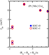
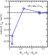
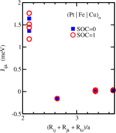
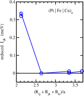
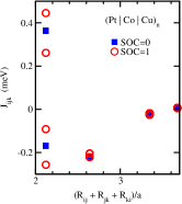
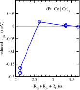
(a)  (b)  (c)  (d)  (e)  (f)

Figure 13: (a),(c),(e) Three-spin exchange interaction parameters $J_{ijk}$ between the 3d-atoms $X$ in (Pt/$X$/Cu)_n multilayer, calculated using Eq. (26) without (closed symbols) and with SOC (open symbols) included, respectively, plotted as a function of the total length for a 3-atomic cluster, $R_{ij}+R_{jk}+R_{ki}$, created by the coupling atoms. (b), (d) and (f) represent the corresponding reduced three-spin interaction parameters $\tilde{J}_{ijk}=J_{ijk}-J_{ikj}$.

Figs. 14 and 15 represent the TCI (a) in comparison with BDMI (b) DMI (c) and isotropic exchange interactions, plotted as a function of energy characterizing the occupation of the valence band (i.e. an artificial Fermi energy position). One can see an oscillating behavior for all parameters when the occupation increases, with their sign changing at different energies because of different origin of these interactions. Note, however, that all quantities shown in Figs. 14 and 15 have a maximum at approximately half occupation of the Mn(Co) $d$-band (see Figs. 14(e) and 15(e)), that correlates also with the maximum of the spin magnetic moment (Figs. 14(a) and 15(a)) and maximum of antiferromagnetic exchange interactions (Figs. 14(d) and 15(d)).

Comparing the $y$- and $z$-components of the BDMI and DMI shown in Figs. 14 (a) and (b), respectively, one can see a more narrow energy region, in which the former quantity has a significant magnitude. Note, however, that the biquadratic interaction is a higher order term in the energy expansion and should represent simultaneously the features of vector and scalar interactions of two spin moments. Thus, plotting in Fig. 14 (a) (thin lines) the function $D^{\alpha}_{ij}(E)J_{ij}(E)/max(J_{ij}(E))$ for the nearest-neighbor interactions, one can see a localization in energy of this function similar to the one seen for the BDMI.

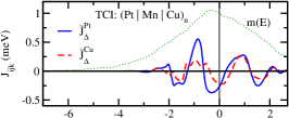
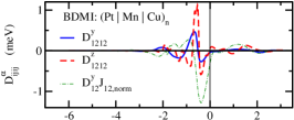
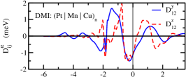
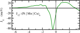
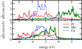
(a)  (b)  (c)  (d)  (e)

Figure 14: Three-spin interaction parameters ${\tilde{J}}_{ijk}(E)$ for the smallest Mn-triangles in (Pt/Mn/Cu)_n multilayer, centered at Cu (${\tilde{J}}^{Cu}_{\Delta}$) and Pt (${\tilde{J}}^{Pt}_{\Delta}$); the dotted line represents the Mn spin magnetic moment $m(E)=M(E)/M_{Mn}$ ($M_{Mn}=3.7\mu_{B}$) as a function of the occupation (a); $y$-, $z$-components of the chiral biquadratic exchange interaction, $\vec{{\cal D}}_{1212}$ (b) and DM interactions, $\vec{D}_{ij}$ (c) between Mn atoms as a function of the occupation; (d) the isotropic exchange $J_{ij}(E)$, and (e) the element-projected DOS(E).

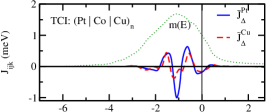
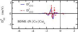
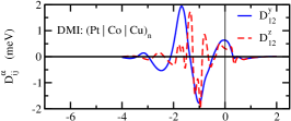
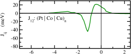
(a)  (b)  (c)  (d)  (e)

Figure 15: Three-spin interaction parameters ${\tilde{J}}_{ijk}(E)$ for the smallest Co-triangles in (Pt/Co/Cu)_n multilayer, centered at Cu (${\tilde{J}}^{Cu}_{\Delta}$) and Pt (${\tilde{J}}^{Pt}_{\Delta}$); the dotted line represents the Co spin magnetic moment $m(E)=M(E)/M_{Co}$ ($M_{Co}=1.9\mu_{B}$) as a function of the occupation (a); $y$-, $z$-components of the chiral biquadratic exchange interaction, $\vec{{\cal D}}_{1212}$ (b) and the DM interactions, $\vec{D}_{ij}$ (c) between Co atoms as a function of the occupation; (d) the isotropic exchange $J_{ij}(E)$, and (e) the element-projected DOS, n(E).

IV.3.2 Monte Carlo simulations

In order to demonstrate a possible impact of the higher-order chiral interactions on the magnetic structure, Monte Carlo simulations have been performed for model systems. We focus here on the effect of the three-spin chiral interactions having rather different properties when compared to the DMI-like interactions. In particular, they depend on the orientation of the coupling spin moments. The calculations have illustrative character, therefore we present only few results showing a non-vanishing impact such interactions, seen here as free parameter, in the formation of the magnetic texture.

Monte Carlo (MC) simulations are performed for 2D lattice having a triangular structure, on the basis of the model Hamiltonian

$$H = -J_{1}\sum_{(i,j)_{1}}\hat{s}_{i}\cdot\hat{s}_{j}$$ (29)

$$-J_{2}\sum_{(i,j)_{2}}\hat{s}_{i}\cdot\hat{s}_{j}-\frac{1}{3}\tilde{J}_{\Delta 1}\sum_{(i,j,k)\in\Delta 1}\hat{s}_{i}\cdot(\hat{s}_{j}\times\hat{s}_{k})\;.$$

Dealing with this expression, the three-spin contribution is evaluated accounting for the counter-clock-wise sequence of atoms $i,j$ and $k$ with $\hat{s}_{i}$, $\hat{s}_{j}$ and $\hat{s}_{k}$ the orientation of the corresponding spin moments respectively. In the model Hamiltonian only the first- (positive) and second-neighbor (negative) isotropic exchange interactions, $J_{1}$ and $J_{2}$, respectively, are taken into account, while the three-spin chiral interactions $\tilde{J}_{\Delta 1}$ are accounted for the smallest possible triangles. To take into account the dependence of the 3-spin interactions on the magnetic configuration we use an algorithm similar to that used to calculate the exchange interactions mediated by non-magnetic components in alloys (e.g. FePd, FeRh, etc.), which also depends on the local magnetic configuration Polesya et al. (2010, 2016). As $\tilde{J}_{\Delta 1}$ depends on the magnetization flux through the triangle, at each MC step they have been calculated according to the discussions above, using the expression $\tilde{J}_{\Delta 1}=\tilde{J}^{0}_{\Delta 1}\hat{n}\cdot(\hat{s}_{i}+\hat{s}_{j}+\hat{s}_{k})$, where $\hat{n}$ is the normal to the film. Here $\tilde{J}^{0}$ is the maximal value of three-spin interaction corresponding to a small deviation of the spin magnetic moments from the collinear direction.

Periodic boundary conditions have been used with the MC cell having $60\times 60$ atomic sites. For the sequential update the Metropolis algorithm has been used. Up to 5000 MC steps have been used to reach the equilibrium. The results represented in Fig. 16 correspond to the temperature $T=0.1$ K. In all cases we used the first-neighbor parameter $J_{1}=3$ meV and rather large value for three-spin interaction parameter $J_{\Delta 1}/J_{1}=1.0$. Fig. 16 shows the magnetic structures for $J_{2}/J_{1}=0$ (a), $J_{2}/J_{1}=-0.25$ (b) and $J_{2}/J_{1}=-0.5$ (c).

(a) (b) (c)

Figure 16: Snapshot ($30\times 30$ atoms) of the magnetic structure obtained by MC simulations for $T=0.1$ K, accounting for first-neighbor $J_{1}$ and second-neighbor $J_{2}$ and three spin $J_{\Delta 1}$ interactions ($J_{\Delta 1}/J_{1}=1.0$) only: (a) $J_{2}=0.0$, (b) $J_{2}/J_{1}=-0.25$, and (c) $J_{2}/J_{1}=-0.5$.

One can see no impact of three-spin interactions on the magnetic structure when the negative second-neighbor interactions are not taken into account. But for systems having competing FM and AFM interactions, the three-spin interactions results in the formation of a vortex structure with the size of the vortexes dependent on relative magnitude of the exchange parameters.

V Summary

To summarize, in the present work we present a general approach to calculate the multispin exchange interactions in order to extend the classical Heisenberg Hamiltonian. This approach allows first principles calculations of multispin interactions in real-space within the framework of the multiple scattering Green function formalism. We discussed some properties of different types of chiral interactions, with the main focus on the three-spin exchange interactions. A specific feature of TCI is its topological origin in contrast to the three-spin DMI-like interactions. We demonstrated by means of MC simulations that this term can lead to a stabilization of vortex-like magnetic texture.

VI Acknowledgement

Financial support by the DFG via SFB 1277 (Emergent Relativistic Effects in Condensed Matter - From Fundamental Aspects to Electronic Functionality).

VII Appendix A

VII.1 Computational details

The numerical results for the coupling parameters are based on first-principles electronic structure calculations performed using the spin-polarized relativistic KKR (SPR-KKR) Green function method H. Ebert et al. (2017); Ebert et al. (2011). The calculations were done in a fully-relativistic mode, except for some special cases pointed out in the manuscript, where scaling of the spin-orbit interaction was applied. All calculations have been performed using the atomic sphere approximation (ASA) within the framework of the local spin density approximation (LSDA) to spin density functional theory (SDFT), using a parametrization for the exchange and correlation potential as given by Vosko et al. Vosko et al. (1980). For the angular momentum expansion of the Green function the angular momentum cutoff $l_{max}=3$ was used.

To demonstrate the properties of multispin interactions, several reference systems have been considered. These are the 3d-metals bcc Fe (lattice parameters $a=5.40$ a.u), fcc Ni ($a=6.65$ a.u.) and hcp Co ($a=4.72$ a.u., $c/a=1.62$), $L1_{0}$ compounds FePt ($a=7.36$ a.u., $c/a=0.95$) and FePd ($a=7.28$ a.u., $c/a=0.96$), as well as the multilayer model systems (Cu/Fe/Pt)_n (Cu/Co/Pt)_n and (Cu/Mn/Pt)_n having fcc structure with (111) orientation of the layers. The lattice parameter $a=7.407$ a.u. was used for all systems. The k-mesh $98\times 98\times 98$ was used for the integration over the BZ of the considered 3d-metals, while $41\times 41\times 41$ was used for the (Cu/$X$/Pt)_n multilayers, and $38\times 38\times 11$ for 1ML Fe(110).

The calculations for 1ML of bcc Fe ($a=5.40$ a.u) have been performed in the supercell geometry with Fe layers separated by three vacuum layers. This decoupling that was sufficient to demonstrate the properties of the exchange interaction parameters for the 2D system.

Another system dealt with is an Fe overlayer on the top of a TMDC compound Fe/1H-TaTe₂ and Fe/1H-WTe₂, with space group $P6_{3}/mmc$ for the bulk TMDC compounds. These calculations have been performed in supercell geometry with the Fe/TMDC films separated by vacuum layers. The lattice parameters are $a=6.82$ a.u. and $c=26.29$ a.u. for 1H-TaTe₂ and $a=6.69$ a.u.and $c=25.71$ a.u. for 1H-WTe₂. More structure information about TMDC monolayers one can find for example in Ref. Ataca et al. (2012).

VIII Appendix B

In the following we present some more details concerning the mapping of the ab-initio magnetic energy to the Heisenberg Hamiltonian. The main idea is demonstrated first dealing with the bilinear interatomic exchange interactions. In order to derive higher-order interactions, rather lengthy transformations are required, which follow similar scheme as that outlined to get the expressions for bilinear interactions.

The expressions for the exchange interaction parameters can be obtained by comparing the energy change due to spin modulations characterized by a wave vector $\vec{q}$, described either in the first-principles formulation or based on the extended Heisenberg model. Obviously, one has to identify the terms having the same dependence on the interatomic distance, in particular by comparing the derivatives with respect to $\vec{q}$-vector in the limit of $q=0$. It may be useful also to select the elements giving zero contributions to the corresponding energy derivatives.

VIII.1 Bilinear terms

VIII.1.1 Spin modulation 1

Let’s start with the bilinear terns in the Heisenberg Hamiltonian:

$$H^{(2)} = -\sum_{i,j}J_{ij}(\hat{s}_{i}\cdot\hat{s}_{j})-\sum_{i,j}\vec{{D}}_{ij}\cdot(\hat{s}_{i}\times\hat{s}_{j})\;.$$ (30)

Depending on the considered interaction parameters different types of spin modulation are used to simplify the derivation. In the present case we use the geometry with the magnetization along the $z$ axis, and the spin spiral having the form

$$\hat{s}_{i} = (\sin\theta\cos(\vec{q}\cdot\vec{R}),\sin\theta\sin(\vec{q}\cdot\vec{R}),\cos\theta)$$ (31)

This leads to the the following energy change for the Heisenberg model

$$\Delta E^{(2)}(\vec{q}) = -\sum_{i,j}J_{ij}(\sin^{2}\theta\cos\vec{q}\cdot(\vec{R}_{j}-\vec{R}_{i})+\cos^{2}\theta-1)-\sum_{i,j}D^{z}_{ij}\sin^{2}\theta\sin\vec{q}\cdot(\vec{R}_{j}-\vec{R}_{i})$$ (32)

$$-\sum_{i,j}D^{x}_{ij}\sin\theta\cos\theta(\sin(\vec{q}\cdot\vec{R}_{i})-\sin(\vec{q}\cdot\vec{R}_{j}))-\sum_{i,j}D^{y}_{ij}\sin\theta\cos\theta(\cos(\vec{q}\cdot\vec{R}_{j})-\cos(\vec{q}\cdot\vec{R}_{i}))\,.$$

Using the relation for the sum over the lattice sites $\vec{R}_{i}$

$$\frac{1}{N}\sum_{i}^{N}e^{-i\vec{q}\cdot\vec{R}_{i}} = \delta_{\vec{q},0}$$ (33)

one can show that the terms due to $D^{x}_{ij}$ and $D^{y}_{ij}$ in the present case do not give contributions to the derivatives with respect to the $\vec{q}$ vector:

$$\sum_{i,j}^{N}D^{y}_{ij}(\cos(\vec{q}\cdot\vec{R}_{j})-\cos(\vec{q}\cdot\vec{R}_{i})) = \sum_{j}^{N}\bigg{[}\sum_{i}^{N}D^{y}_{ij}\bigg{]}\cos(\vec{q}\cdot\vec{R}_{j})-\sum_{i}^{N}\bigg{[}\sum_{j}^{N}D^{y}_{ij}\bigg{]}\cos(\vec{q}\cdot\vec{R}_{i})=ND^{y}_{0}(\delta_{\vec{q},0}-\delta_{\vec{q},0})=0$$ (34)

and

$$\sum_{i,j}^{N}D^{x}_{ij}(\sin(\vec{q}\cdot\vec{R}_{j})-\sin(\vec{q}\cdot\vec{R}_{i})) = \sum_{j}^{N}\bigg{[}\sum_{i}^{N}D^{x}_{ij}\bigg{]}\sin(\vec{q}\cdot\vec{R}_{j})-\sum_{i}^{N}\bigg{[}\sum_{j}^{N}D^{x}_{ij}\bigg{]}\sin(\vec{q}\cdot\vec{R}_{i})=0\,,$$ (35)

taking into account that the sum over $i(j)$ in square brackets in these expressions gives the same value for each site $j(i)$.

Taking the first- and second-order derivatives of the energy change $\Delta E(\vec{q})$ (Eq. (32)) with respect to $\vec{q}$, one obtains the expressions contributed either by the DMI interactions

$$\frac{\partial}{\partial\vec{q}}\Delta E(\vec{q})\bigg{|}_{q\to 0} = -\sin^{2}\theta\sum_{i\neq j}^{N}D^{z}_{ij}\hat{q}\cdot(\vec{R}_{i}-\vec{R}_{j})$$ (36)

or by the isotropic exchange interaction

$$\frac{\partial^{2}}{\partial\vec{q}^{2}}\Delta E(\vec{q})\bigg{|}_{q\to 0} = \sin^{2}\theta\sum_{i,j}J_{ij}(\hat{q}\cdot(\vec{R}_{i}-\vec{R}_{j}))^{2}$$ (37)

with $\hat{q}=\vec{q}/|\vec{q}|$ the unit vector giving the direction of the wave vector $\vec{q}$.

Now let’s consider the first-principles energy change due to a spin spiral, evaluated in terms of the Green function

$$\Delta{\cal E}^{(2)} = -\frac{1}{\pi}\mbox{Im}\,\mbox{Tr}\int^{E_{F}}dE\,\Delta VG_{0}\Delta VG_{0}\;.$$ (38)

Substituting the multiple-scattering representation for the Green function into this equation together with the perturbation

$$\Delta V(\vec{r}) = \sum_{i}\beta\big{(}\vec{\sigma}\cdot\hat{s}_{i}-\sigma_{z}\big{)}B_{xc}(\vec{r})\;,$$ (39)

for a spin spiral according to Eq. (31), and introducing the definition

$${\cal J}^{\alpha\beta}_{ij} = \frac{1}{2\pi}\mbox{Im}\,\mbox{Tr}\int^{E_{F}}dE\,T^{\alpha}_{i}\tau_{ij}T^{\beta}_{j}\tau_{ji}\,,$$ (40)

we obtain the following symmetrized expressions for the energy change

$$\Delta{\cal E}^{(2)} = \sum_{i,j}\sin^{2}\theta\bigg{[}\frac{1}{2}({\cal J}^{xx}_{ij}+{\cal J}^{yy}_{ij})\cos\vec{q}\cdot(\vec{R}_{i}-\vec{R}_{j})+{\cal J}^{zz}_{ij}(\cos\theta-1)^{2}\bigg{]}$$ (41)

$$+\sin^{2}\theta\frac{1}{2}({\cal J}^{xx}_{ij}-{\cal J}^{yy}_{ij})\cos\vec{q}\cdot(\vec{R}_{i}+\vec{R}_{j})$$

$$+\sin^{2}\theta\frac{1}{2}({\cal J}^{xy}_{ij}+{\cal J}^{yx}_{ij})\sin\vec{q}\cdot(\vec{R}_{i}+\vec{R}_{j})$$

$$+\sin^{2}\theta\frac{1}{2}({\cal J}^{xy}_{ij}-{\cal J}^{yx}_{ij})\sin\vec{q}\cdot(\vec{R}_{j}-\vec{R}_{i})$$

$$+\sin\theta(\cos\theta-1)[{\cal J}^{xz}_{ij}\cos(\vec{q}\cdot\vec{R}_{i})+{\cal J}^{zx}_{ij}\cos(\vec{q}\cdot\vec{R}_{j})]$$

$$+\sin\theta(\cos\theta-1)[{\cal J}^{yz}_{ij}\sin(\vec{q}\cdot\vec{R}_{i})+{\cal J}^{zy}_{ij}\sin(\vec{q}\cdot\vec{R}_{j})]\,.$$

In Eq. (40) we use $T^{\alpha}_{i}=\langle Z_{i}|\beta\sigma^{\alpha}B_{xc,i}|Z_{i}\rangle$ and the prefactor $1/2$ prevents a double counting of contribution to the energy associated with a pair of atoms.

Using again Eq. (33) for the sum over the lattice sites $\vec{R}_{i}$ one can show that the derivatives with respect to $\vec{q}$ of the off-diagonal terms associated with $J^{\alpha z}_{ij}$ and $J^{z\alpha}_{ij}$ parameters vanish.

For instance, one finds:

$$\sum_{i,j}^{N}{\cal J}^{yz}_{ij}\sin(\vec{q}\cdot\vec{R}_{i}) = -\frac{i}{2}\sum_{i}^{N}\bigg{[}\sum_{j}{\cal J}^{yz}_{ij}\bigg{]}(e^{i(\vec{q}\cdot\vec{R}_{i})}-e^{-i(\vec{q}\cdot\vec{R}_{i})})$$ (42)

$$= -\frac{i}{2}{\cal J}^{yz}_{0}\sum_{i}^{N}(e^{i(\vec{q}\cdot\vec{R}_{i})}-e^{-i(\vec{q}\cdot\vec{R}_{i})})=-\frac{i}{2}NJ^{yz}_{0}(\delta_{\vec{q},0}-\delta_{\vec{q},0})=0$$

since the sum $\sum_{j}J^{\alpha\beta}_{ij}=J^{\alpha\beta}_{0}$ is the same for all sites $i$. For the other term one finds

$$\sum_{i,j}^{N}{\cal J}^{xz}_{ij}\cos(\vec{q}\cdot\vec{R}_{i}) = \frac{N}{2}{\cal J}^{xz}_{0}\delta_{\vec{q},0}$$ (43)

This value does not depend on $q$. As a result, its derivative with respect to $\vec{q}$, used to derive the expression for the exchange parameters, vanishes. The same concerns also the exchange parameters ${\cal J}^{zy}$ and ${\cal J}^{zx}$.

Transforming the term proportional to $({\cal J}^{xy}_{ij}+{\cal J}^{yx}_{ij})$ and using again Eq. (33), one obtains

$$\sum_{i,j}^{N}({\cal J}^{xy}_{ij}+{\cal J}^{yx}_{ij})\sin\vec{q}\cdot(\vec{R}_{i}+\vec{R}_{j}) = \sum_{i,j}^{N}({\cal J}^{xy}_{ij}+{\cal J}^{yx}_{ij})(\cos(\vec{q}\cdot(\vec{R}_{i}-\vec{R}_{j})\sin(2\vec{q}\cdot\vec{R}_{j})+\sin(\vec{q}\cdot(\vec{R}_{i}-\vec{R}_{j})\cos(2\vec{q}\cdot\vec{R}_{j}))$$ (44)

$$= \sum_{i}^{N}\bigg{[}\sum_{j}^{N}({\cal J}^{xy}_{ij}+{\cal J}^{yx}_{ij})\cos(\vec{q}\cdot(\vec{R}_{i}-\vec{R}_{j}))\bigg{]}\sin(2\vec{q}\cdot\vec{R}_{i})$$

$$+\sum_{i}^{N}\bigg{[}\sum_{j}^{N}({\cal J}^{xy}_{ij}+{\cal J}^{yx}_{ij})\sin(\vec{q}\cdot(\vec{R}_{i}-\vec{R}_{j}))\bigg{]}\cos(2\vec{q}\cdot\vec{R}_{i}))=const\,,$$

where the first sum vanishes due to the summation over $i$, sum does not depend on $q$. The same behavior is shown by the term proportional to $({\cal J}^{xx}_{ij}-{\cal J}^{yy}_{ij})$

Taking the first- and second-order derivatives of the energy change $\Delta{\cal E}^{(2)}(\vec{q})$ with respect to $\vec{q}$, Eq. (41) leads to the expressions contributed either by the DMI interactions

$$\frac{\partial}{\partial\vec{q}}\Delta{\cal E}^{(2)}(\vec{q})\bigg{|}_{q\to 0} = -\sin^{2}\theta\sum_{i\neq j}^{N}\frac{1}{2}({\cal J}^{xy}_{ij}-{\cal J}^{yx}_{ij})\hat{q}\cdot(\vec{R}_{i}-\vec{R}_{j})$$ (45)

and the isotropic exchange

$$\frac{\partial^{2}}{\partial\vec{q}^{2}}\Delta{\cal E}^{(2)}(\vec{q})\bigg{|}_{q\to 0} = \sin^{2}\theta\sum_{i\neq j}^{N}\frac{1}{2}({\cal J}^{xx}_{ij}+{\cal J}^{yy}_{ij})(\hat{q}\cdot(\vec{R}_{i}-\vec{R}_{j}))^{2}\,.$$ (46)

Comparing these equations with the Eqs. (36)-(37), one obtains for the DMI

$$D^{z}_{ij} = \frac{1}{2}({\cal J}^{xy}_{ij}-{\cal J}^{yx}_{ij})$$ (47)

and for the isotropic exchange

$$J_{ij} = \frac{1}{2}({\cal J}^{xx}_{ij}+{\cal J}^{yy}_{ij})\,.$$ (48)

The two others DMI components are discussed in detail in previous works Mankovsky and Ebert (2017); Mankovsky et al. (2019).

VIII.1.2 Spin modulation 2

For comparison, we use here also the spin modulation within the $xy$-plane, characterized by two q-vectors:

$$\hat{s}_{i} = (\mbox{sin}(\vec{q}_{1}\cdot\vec{R}_{i})\;\mbox{cos}(\vec{q}_{2}\cdot\vec{R}_{i})\;,\mbox{sin}(\vec{q}_{2}\cdot\vec{R}_{i})\;,\mbox{cos}(\vec{q}_{1}\cdot\vec{R}_{i})\mbox{cos}(\vec{q}_{2}\cdot\vec{R}_{i}))\;.$$ (49)

The corresponding results can be used later to derive the three-spin and biquadratic DMI-like interactions.

Within the Heisenberg model the second order terms associated with the isotropic exchange interaction are given by

$$\Delta{E}^{(2)} = -\sum_{i,j}J_{ij}[(\hat{s}_{i}\cdot\hat{s}_{j})-1]$$ (50)

$$= -\sum_{i,j}J_{ij}\bigg{[}\cos\vec{q}_{1}\cdot(\vec{R}_{j}-\vec{R}_{j})\cos(\vec{q}_{2}\cdot\vec{R}_{i})\cos(\vec{q}_{2}\cdot\vec{R}_{j})+\sin(\vec{q}_{2}\cdot\vec{R}_{i})\sin(\vec{q}_{2}\cdot\vec{R}_{j})-1\bigg{]}$$

Taking $q_{1}=0$, the second-order derivative of the energy with respect to $q_{2}$ is given by

$$\frac{\partial^{2}}{\partial\vec{q}_{2}^{2}}\Delta{\cal E}^{(2)} = \sum_{i,j}J_{ij}(\hat{q}\cdot(\vec{R}_{j}-\vec{R}_{i}))^{2}$$ (51)

On the other hand, taking $q_{2}=0$, the second-order derivative of the energy with respect to $q_{1}$ has the form

$$\frac{\partial^{2}}{\partial\vec{q}_{1}^{2}}\Delta{\cal E}^{(2)} = \sum_{i,j}J_{ij}(\hat{q}\cdot(\vec{R}_{j}-\vec{R}_{i}))^{2}\,.$$ (52)

In the first-principles approach, substituting the perturbation due to the spin modulation according to Eq. (49) and using the definition in Eq. (40) one obtains

$$\Delta{\cal E}^{(2)} = -\sum_{i,j}{\cal J}^{xx}_{ij}\sin(\vec{q}_{1}\cdot\vec{R}_{i})\cos(\vec{q}_{2}\cdot\vec{R}_{i})\sin(\vec{q}_{1}\cdot\vec{R}_{j})\cos(\vec{q}_{2}\cdot\vec{R}_{j})+{\cal J}^{yy}_{ij}\sin(\vec{q}_{2}\cdot\vec{R}_{i})\sin(\vec{q}_{2}\cdot\vec{R}_{j})$$ (53)

$$+{\cal J}^{zz}_{ij}(\cos(\vec{q}_{1}\cdot\vec{R}_{i})\cos(\vec{q}_{2}\cdot\vec{R}_{i})-1)(\cos(\vec{q}_{1}\cdot\vec{R}_{i})\cos(\vec{q}_{2}\cdot\vec{R}_{i})-1)$$

$$+{\cal J}^{xy}_{ij}\sin(\vec{q}_{1}\cdot\vec{R}_{i})\cos(\vec{q}_{2}\cdot\vec{R}_{i})\sin(\vec{q}_{2}\cdot\vec{R}_{j})+{\cal J}^{yx}_{ij}\sin(\vec{q}_{2}\cdot\vec{R}_{i})\sin(\vec{q}_{2}\cdot\vec{R}_{j})\cos(\vec{q}_{2}\cdot\vec{R}_{j})$$

$$+{\cal J}^{xz}_{ij}\sin(\vec{q}_{1}\cdot\vec{R}_{i})\cos(\vec{q}_{2}\cdot\vec{R}_{i})(\cos(\vec{q}_{1}\cdot\vec{R}_{j})\cos(\vec{q}_{2}\cdot\vec{R}_{j})-1)$$

$$+{\cal J}^{zx}_{ij}(\cos(\vec{q}_{1}\cdot\vec{R}_{i})\cos(\vec{q}_{2}\cdot\vec{R}_{i})-1)\sin(\vec{q}_{1}\cdot\vec{R}_{j})\cos(\vec{q}_{2}\cdot\vec{R}_{j})$$

$$+{\cal J}^{yz}_{ij}\sin(\vec{q}_{2}\cdot\vec{R}_{i})(\cos(\vec{q}_{1}\cdot\vec{R}_{j})\cos(\vec{q}_{2}\cdot\vec{R}_{j})-1)+{\cal J}^{zy}_{ij}(\cos(\vec{q}_{1}\cdot\vec{R}_{i})\cos(\vec{q}_{2}\cdot\vec{R}_{i})-1)\sin(\vec{q}_{2}\cdot\vec{R}_{j})\;.$$

One can show that all off-diagonal terms w.r.t. the spatial directions $(x,y,z)$ in this expression do not contribute to the derivatives with respect to the wave vector.

Omitting the terms giving no contribution to the second-order derivatives with respect to $\vec{q}$, one obtains after some transformations the expression

$$\Delta{\cal E}^{(2)} = \frac{1}{2}\sum_{i,j}\bigg{[}\Bigg{(}{\cal J}^{xx}_{ij}\cos\;(\vec{q}_{1}\cdot(\vec{R}_{i}-\vec{R}_{j}))+{\cal J}^{yy}_{ij}\Bigg{)}\cos\;(\vec{q}_{2}\cdot(\vec{R}_{i}-\vec{R}_{j}))$$ (54)

$$+\Bigg{(}{\cal J}^{xx}_{ij}\cos\;(\vec{q}_{1}\cdot(\vec{R}_{i}-\vec{R}_{j}))-{\cal J}^{yy}_{ij}\Bigg{)}\cos\;(\vec{q}_{2}\cdot(\vec{R}_{i}+\vec{R}_{j}))+...\bigg{]}\;$$

The second term does not contribute to the q-dependence of the energy (see discussion above). Taking $q_{1}=0$ and evaluating the second-order derivative of the energy with respect to $\vec{q}_{2}$ one obtains

$$\frac{\partial^{2}}{\partial q_{2}^{2}}\Delta{\cal E}^{(2)} = \frac{1}{2}\sum_{i,j}(\hat{q}\cdot(\vec{R}_{j}-\vec{R}_{i}))^{2}({\cal J}^{xx}_{ij}+{\cal J}^{yy}_{ij})\;.$$ (55)

Comparing this expression with the corresponding expression obtained for the Heisenberg model leads to the expression for isotropic exchange parameter given by Eq. (48), showing that both modulations lead to the same result.

VIII.2 Fourth-order interactions

VIII.2.1 Four-spin isotropic interactions. z-component of DMI-like exchnage interactions

Next, we consider four-spin terms. First, we will deal with the isotropic exchange interaction and DMI-like terms in the extended Heisenberg Hamiltonian

$$H^{(4)} = -\sum_{i,j,k,l}\bigg{[}J^{s}_{ijkl}(\hat{s}_{i}\cdot\hat{s}_{j})(\hat{s}_{k}\cdot\hat{s}_{l})+\vec{\cal D}_{ijkl}\cdot(\hat{s}_{i}\times\hat{s}_{j})(\hat{s}_{k}\cdot\hat{s}_{l})\bigg{]}\;.$$ (56)

For the sake of convenience we keep only the terms required to derive the expressions for the isotropic and DMI-like (only z-component) exchange coupling parameters, following the same idea as used to derive the bilinear exchange parameters. The FM state with the magnetization along the $z$ axis is used as a reference state for a spin-spiral characterized by the vector $\vec{q}$ leading to a $q$-dependent energy change. The terms associated with the isotropic exchange interactions $J^{s}_{ijkl}$ are proportional to $q^{4}$. On the other hand, the terms proportional to $q^{3}$ are associated with the DMI-like interactions ${\cal D}^{z}_{ijkl}$, i.e. they depend on vector product and scalar product of two pairs of spin moments. We focus here on these terms, for which we can find a one to one correspondence between the model and first-principles energy terms. Following the idea used to derive the bilinear terms, for the sake of simplicity we consider now only the terms giving raise to a q-dependence of the energy. In this case, the Hamiltonian can be written as follows

$$H^{(4)} = -\sum_{i,j,k,l}\bigg{[}J^{s}_{ijkl}(s^{x}_{i}s^{x}_{j}+s^{y}_{i}s^{y}_{j})(s^{x}_{k}s^{x}_{l}+s^{y}_{k}s^{y}_{l})$$ (57)

$$+{\cal D}^{z}_{ijkl}(s^{x}_{i}s^{y}_{j}-s^{y}_{i}s^{x}_{j})(s^{x}_{k}s^{x}_{l}+s^{y}_{k}s^{y}_{l})+...\bigg{]}\;,$$

with the summation over all sites in the lattice with $i\neq j$ and $k\neq l$. A similar summation occurs also for the first-principles approach, leading to a one-to-one correspondence between various terms in the two approaches. In the following, however, we will focus at the end on the three-spin and biquadratic interactions.

Using the spin modulation in the following form

$$\hat{s}_{i} = (\mbox{sin}\theta\,\mbox{cos}(\vec{q}\cdot\vec{R}_{i}),\mbox{sin}\theta\,\mbox{sin}(\vec{q}\,\cdot\vec{R}_{i}),\mbox{cos}\theta)$$ (58)

the corresponding energy change within the Heisenberg model is given by

$$\Delta E^{(4)} = -\sum_{i,j,k,l}\bigg{[}J^{s}_{ijkl}\;\mbox{sin}^{4}\theta\;\mbox{cos}\vec{q}\cdot(\vec{R}_{i}-\vec{R}_{j})\;\mbox{cos}\vec{q}\cdot(\vec{R}_{k}-\vec{R}_{l})$$ (59)

$$+D^{z}_{ijkl}\;\mbox{sin}^{4}\theta\;\mbox{sin}\vec{q}\cdot(\vec{R}_{i}-\vec{R}_{j})\;\mbox{cos}\vec{q}\cdot(\vec{R}_{k}-\vec{R}_{l})+...\bigg{]}\;.$$

In order to derive the expressions for the isotropic and DMI-like interaction parameters, we consider the energy derivatives $\frac{\partial^{2}}{\partial q^{2}}\frac{\partial^{2}}{\partial q^{2}}\Delta E^{(4)}$ and $\frac{\partial}{\partial q}\frac{\partial^{2}}{\partial q^{2}}\Delta E^{(4)}$ in the limit of $q=0$. These derivatives are applied to the terms corresponding to different pairs of spin moments. As a results, one obtains:

$$\frac{\partial}{\partial q}\frac{\partial^{2}}{\partial q^{2}}\bigg{|}_{q\to 0}\Delta E^{(4)} = \sum_{i,j,k,l}{\cal D}^{z}_{ijkl}\;\mbox{sin}^{4}\theta\;(\vec{R}_{i}-\vec{R}_{j})(\vec{R}_{k}-\vec{R}_{l})^{2}\;,$$ (60)

and the fourth-order derivative terms

$$\frac{\partial^{2}}{\partial q^{2}}\frac{\partial^{2}}{\partial q^{2}}\bigg{|}_{q\to 0}\Delta E^{(4)} = -\sum_{i,j,k,l}J^{s}_{ijkl}\;\mbox{sin}^{4}\theta\;(\vec{R}_{i}-\vec{R}_{j})^{2}(\vec{R}_{k}-\vec{R}_{l})^{2}\;,$$ (61)

Note that we do not consider in the last expression the terms $\sim(\vec{R}_{k}-\vec{R}_{l})^{4}$ or $\sim(\vec{R}_{i}-\vec{R}_{j})^{4}$, which do not contribute to the q-dependence of the energy which is associated with the second pair of spin moments.

Next, we evaluate the first-principles energy change due to the same spin spiral. For this purpose we use the fourth-order energy term with respect to the perturbation.

$$\Delta{\cal E}^{(4)} = -\frac{1}{\pi}\sum_{i,j,k,l}\mbox{Im}\,\mbox{Tr}\int^{E_{F}}dE\,\Delta VG\Delta VG\Delta VG\Delta VG\;$$ (62)

$$= -\frac{1}{\pi}\sum_{i,j,k,l}\mbox{Im}\,\mbox{Tr}\int^{E_{F}}dE\,$$

$$\times\langle Z_{i}|\Delta V|Z_{i}\rangle\tau_{ij}\langle Z_{j}|\Delta V|Z_{j}\rangle\tau_{jk}\langle Z_{k}|\Delta V|Z_{k}\rangle\tau_{kl}\langle Z_{l}|\Delta V|Z_{l}\rangle\tau_{li}\;.$$

Using the spin-spiral according to Eq. (58) and keeping only terms leading to derivatives in the form of Eqs. (60) and (61), we obtain

$$\Delta{\cal E}^{(4)} = -\frac{1}{\pi}\sum_{i,j,k,l}\mbox{Im}\,\mbox{Tr}\int^{E_{F}}dE\,\mbox{sin}^{4}\theta$$ (63)

$$\times\bigg{[}T^{x}_{i}\tau_{ij}T^{x}_{j}\tau_{jk}T^{x}_{k}\tau_{kl}T^{x}_{l}\tau_{li}\;\mbox{cos}(\vec{q}\cdot\vec{R}_{i})\,\mbox{cos}(\vec{q}\cdot\vec{R}_{j})\,\mbox{cos}(\vec{q}\cdot\vec{R}_{k})\,\mbox{cos}(\vec{q}\cdot\vec{R}_{l})$$

$$+T^{x}_{i}\tau_{ij}T^{x}_{j}\tau_{jk}T^{y}_{k}\tau_{kl}T^{y}_{l}\tau_{li}\;\mbox{cos}(\vec{q}\cdot\vec{R}_{i})\,\mbox{cos}(\vec{q}\cdot\vec{R}_{j})\,\mbox{sin}(\vec{q}\cdot\vec{R}_{k})\,\mbox{sin}\vec{q}\cdot\vec{R}_{l})$$

$$+T^{y}_{i}\tau_{ij}T^{y}_{j}\tau_{jk}T^{x}_{k}\tau_{kl}T^{x}_{l}\tau_{li}\;\mbox{sin}(\vec{q}\cdot\vec{R}_{i})\,\mbox{sin}(\vec{q}\cdot\vec{R}_{j})\,\mbox{cos}(\vec{q}\cdot\vec{R}_{k})\,\mbox{cos}(\vec{q}\cdot\vec{R}_{l})$$

$$+T^{y}_{i}\tau_{ij}T^{y}_{j}\tau_{jk}T^{y}_{k}\tau_{kl}T^{y}_{l}\tau_{li}\;\mbox{sin}(\vec{q}\cdot\vec{R}_{i})\,\mbox{sin}(\vec{q}\cdot\vec{R}_{j})\,\mbox{sin}(\vec{q}\cdot\vec{R}_{k})\,\mbox{sin}(\vec{q}\cdot\vec{R}_{l})$$

$$+T^{x}_{i}\tau_{ij}T^{y}_{j}\tau_{jk}T^{x}_{k}\tau_{kl}T^{x}_{l}\tau_{li}\;\mbox{cos}(\vec{q}\cdot\vec{R}_{i})\,\mbox{sin}(\vec{q}\cdot\vec{R}_{j})\,\mbox{cos}(\vec{q}\cdot\vec{R}_{k})\,\mbox{cos}(\vec{q}\cdot\vec{R}_{l})$$

$$+T^{y}_{i}\tau_{ij}T^{x}_{j}\tau_{jk}T^{y}_{k}\tau_{kl}T^{y}_{l}\tau_{li}\;\mbox{sin}(\vec{q}\cdot\vec{R}_{i})\,\mbox{cos}(\vec{q}\cdot\vec{R}_{j})\,\mbox{sin}(\vec{q}\cdot\vec{R}_{k})\,\mbox{sin}\vec{q}\cdot\vec{R}_{l})$$

$$+T^{y}_{i}\tau_{ij}T^{x}_{j}\tau_{jk}T^{x}_{k}\tau_{kl}T^{x}_{l}\tau_{li}\;\mbox{sin}(\vec{q}\cdot\vec{R}_{i})\,\mbox{cos}(\vec{q}\cdot\vec{R}_{j})\,\mbox{cos}(\vec{q}\cdot\vec{R}_{k})\,\mbox{cos}(\vec{q}\cdot\vec{R}_{l})$$

$$+T^{x}_{i}\tau_{ij}T^{y}_{j}\tau_{jk}T^{y}_{k}\tau_{kl}T^{y}_{l}\tau_{li}\;\mbox{cos}(\vec{q}\cdot\vec{R}_{i})\,\mbox{sin}(\vec{q}\cdot\vec{R}_{j})\,\mbox{sin}(\vec{q}\cdot\vec{R}_{k})\,\mbox{sin}(\vec{q}\cdot\vec{R}_{l})+...\bigg{]}$$

By using the definition

$${\cal J}_{ijkl}^{\alpha\beta\gamma\delta} = \frac{1}{2\pi}\mbox{Im}\,\mbox{Tr}\int^{E_{F}}dE\,T^{\alpha}_{i}\tau_{ij}T^{\beta}_{j}\tau_{jk}T^{\gamma}_{k}\tau_{kl}T^{\delta}_{l}\tau_{li}$$ (64)

with a factor $\frac{1}{2}$ to have the same form for the biquadratic term in the Hamiltonian, as the bilinear term has, one gets after some transformations the expression

$$\Delta{\cal E}^{(4)} = -\frac{1}{4}\sum_{i,j,k,l}\mbox{sin}^{4}\theta$$ (65)

$$\times\bigg{[}({\cal J}_{ijkl}^{xxxx}+{\cal J}_{ijkl}^{xxyy}+{\cal J}_{ijkl}^{yyxx}+{\cal J}_{ijkl}^{yyyy})\;\mbox{cos}(\vec{q}\cdot(\vec{R}_{i}-\vec{R}_{j}))\,\mbox{cos}(\vec{q}\cdot(\vec{R}_{k}-\vec{R}_{l}))$$

$$+({\cal J}_{ijkl}^{xxxx}+{\cal J}_{ijkl}^{xxyy}-{\cal J}_{ijkl}^{yyxx}-{\cal J}_{ijkl}^{yyyy})\;\mbox{cos}(\vec{q}\cdot(\vec{R}_{i}+\vec{R}_{j}))\,\mbox{cos}(\vec{q}\cdot(\vec{R}_{k}-\vec{R}_{l}))$$

$$+({\cal J}_{ijkl}^{xxxx}-{\cal J}_{ijkl}^{xxyy}+{\cal J}_{ijkl}^{yyxx}-{\cal J}_{ijkl}^{yyyy})\;\mbox{cos}(\vec{q}\cdot(\vec{R}_{i}-\vec{R}_{j}))\,\mbox{cos}(\vec{q}\cdot(\vec{R}_{k}+\vec{R}_{l}))$$

$$+({\cal J}_{ijkl}^{xxxx}-{\cal J}_{ijkl}^{xxyy}-{\cal J}_{ijkl}^{yyxx}+{\cal J}_{ijkl}^{yyyy})\;\mbox{cos}(\vec{q}\cdot(\vec{R}_{i}+\vec{R}_{j}))\,\mbox{cos}(\vec{q}\cdot(\vec{R}_{k}+\vec{R}_{l}))$$

$$+({\cal J}_{ijkl}^{xyxx}+{\cal J}_{ijkl}^{xyyy}-{\cal J}_{ijkl}^{yxxx}-{\cal J}_{ijkl}^{yxyy}))\;\mbox{sin}(\vec{q}\cdot(\vec{R}_{i}-\vec{R}_{j}))\,\mbox{cos}(\vec{q}\cdot(\vec{R}_{k}-\vec{R}_{l}))$$

$$+({\cal J}_{ijkl}^{xyxx}+{\cal J}_{ijkl}^{xyyy}+{\cal J}_{ijkl}^{yxxx}+{\cal J}_{ijkl}^{yxyy})\;\mbox{sin}(\vec{q}\cdot(\vec{R}_{i}+\vec{R}_{j}))\,\mbox{cos}(\vec{q}\cdot(\vec{R}_{k}-\vec{R}_{l}))$$

$$+({\cal J}_{ijkl}^{xyxx}-{\cal J}_{ijkl}^{xyyy}+{\cal J}_{ijkl}^{yxxx}-{\cal J}_{ijkl}^{yxyy})\;\mbox{sin}(\vec{q}\cdot(\vec{R}_{i}-\vec{R}_{j}))\,\mbox{cos}(\vec{q}\cdot(\vec{R}_{k}+\vec{R}_{l}))$$

$$+({\cal J}_{ijkl}^{xyxx}-{\cal J}_{ijkl}^{xyyy}-{\cal J}_{ijkl}^{yxxx}+{\cal J}_{ijkl}^{yxyy})\;\mbox{sin}(\vec{q}\cdot(\vec{R}_{i}+\vec{R}_{j}))\,\mbox{cos}(\vec{q}\cdot(\vec{R}_{k}+\vec{R}_{l}))+...\bigg{]}$$

Evaluating the derivatives $\frac{\partial}{\partial q}\frac{\partial^{2}}{\partial q^{2}}\Delta{\cal E}^{(4)}$ and $\frac{\partial^{2}}{\partial q^{2}}\frac{\partial^{2}}{\partial q^{2}}\Delta{\cal E}^{(4)}$ in the limit $q=0$, and equating to corresponding terms in Eqs. (60) and (61), one obtains

$$J_{ijkl}^{s} = \frac{1}{4}\bigg{[}({\cal J}_{ijkl}^{xxxx}+{\cal J}_{ijkl}^{xxyy}+{\cal J}_{ijkl}^{yyxx}+{\cal J}_{ijkl}^{yyyy}))\bigg{]}$$ (66)

$$D_{ijkl}^{z} = \frac{1}{4}\bigg{[}{\cal J}_{ijkl}^{xyxx}+{\cal J}_{ijkl}^{xyyy}-{\cal J}_{ijkl}^{yxxx}-{\cal J}_{ijkl}^{yxyy})\;\bigg{]}$$ (67)

VIII.2.2 Biquadratic and 3-spin DMI-like interactions: x- and y- components

To obtain the $x$- and $y$-components of the 4-spin DMI-like interactions we will follow the scheme used to derive the corresponding components of the bilinear DMI. The corresponding term in the Heisenberg Hamiltonian has the form

$${H}^{a(4)} = -\sum_{i,j,k,l}\vec{{\cal D}}_{ijkl}\cdot(\hat{s}_{i}\times\hat{s}_{j})(\hat{s}_{k}\cdot\hat{s}_{l})\;.$$ (68)

Here we use the spin modulation characterized by two $\vec{q}$-vectors, which allows the simultaneous tilting of spin moments towards the $x$- and $y$-axes:

$$\hat{s}_{i} = (\mbox{sin}(\vec{q}_{1}\cdot\vec{R}_{i})\;\mbox{cos}(\vec{q}_{2}\cdot\vec{R}_{i})\,,\;\mbox{sin}(\vec{q}_{2}\cdot\vec{R}_{i})\,,\;\mbox{cos}(\vec{q}_{1}\cdot\vec{R}_{i})\mbox{cos}(\vec{q}_{2}\cdot\vec{R}_{i}))\;,$$ (69)

The corresponding contribution to the energy in model approach is now:

$$\Delta{E}^{a(4)} = -\sum_{i,j,k,l}\bigg{[}{\cal D}^{x}_{ijkl}[\mbox{sin}(\vec{q}_{2}\cdot\vec{R}_{i})\,\mbox{cos}(\vec{q}_{1}\cdot\vec{R}_{j})\mbox{cos}(\vec{q}_{2}\cdot\vec{R}_{j})-\mbox{sin}(\vec{q}_{2}\cdot\vec{R}_{j})\,\mbox{cos}(\vec{q}_{1}\cdot\vec{R}_{i})\,\mbox{cos}(\vec{q}_{2}\cdot\vec{R}_{i})]$$ (70)

$$+{\cal D}^{y}_{ijkl}\;\mbox{sin}(\vec{q}_{1}\cdot(\vec{R}_{j}-\vec{R}_{i}))\;\mbox{cos}(\vec{q}_{2}\cdot\vec{R}_{i})\;\mbox{cos}(\vec{q}_{2}\cdot\vec{R}_{j})$$

$$+{\cal D}^{z}_{ijkl}[\mbox{sin}(\vec{q}_{1}\cdot\vec{R}_{i})\,\mbox{cos}(\vec{q}_{2}\cdot\vec{R}_{i})\,\mbox{sin}(\vec{q}_{2}\cdot\vec{R}_{j})-\mbox{sin}(\vec{q}_{1}\cdot\vec{R}_{j})\,\mbox{cos}(\vec{q}_{2}\cdot\vec{R}_{j})\,\mbox{sin}(\vec{q}_{2}\cdot\vec{R}_{i})]\bigg{]}$$

$$\times[\mbox{cos}(\vec{q}_{1}\cdot(\vec{R}_{k}-\vec{R}_{l}))\,\mbox{cos}(\vec{q}_{2}\cdot\vec{R}_{k})\,\mbox{cos}(\vec{q}_{2}\cdot\vec{R}_{l})+\mbox{sin}(\vec{q}_{2}\cdot\vec{R}_{k})\,\mbox{sin}(\vec{q}_{2}\cdot\vec{R}_{l})]\,.$$

The 4-spin DMI-like terms involve a cross-product of the spin moments on sites $i$ and $j$ and a scalar product of the spin moments on sites $k$ and $l$. Therefore, to derive the expression for the exchange parameters, one has to consider the first-order derivative with respect to the wave vector of the part associated with the atoms $i$ and $j$ and the second order derivative of the part associated with the atoms $k$ and $l$. Taking first $q_{1}=0$, one obtains

$$\frac{\partial}{\partial q_{2}}\frac{\partial^{2}}{\partial q_{2}^{2}}\bigg{|}_{q_{2}=0}\Delta{E}^{a(4)} = \sum_{i,j,k,l}{\cal D}^{x}_{ijkl}\,({\hat{q}_{2}}\cdot(\vec{R}_{j}-\vec{R}_{i}))\,({\hat{q}_{2}}\cdot(\vec{R}_{k}-\vec{R}_{l}))^{2}\,.$$ (71)

Calculating alternatively first derivatives $\frac{\partial}{\partial q_{1}}|_{q_{1}=0}\Delta{E}^{a(4)}$ and then $\frac{\partial^{2}}{\partial q_{2}^{2}}|_{q_{2}=0}\Delta{E}^{a(4)}$, one obtains

$$\frac{\partial}{\partial q_{1}}\bigg{|}_{q_{1}=0}\frac{\partial^{2}}{\partial q_{2}^{2}}\bigg{|}_{q_{2}=0}\Delta{E}^{a(4)} = \sum_{i,j,k,l}{\cal D}^{y}_{ijkl}\,({\hat{q}_{1}}\cdot(\vec{R}_{j}-\vec{R}_{i}))\,({\hat{q}_{2}}\cdot(\vec{R}_{k}-\vec{R}_{l}))^{2}$$ (72)

In the case $l=j$ we obtain the three-spin interactions, while in the case $l=j,k=i$ we will get the DMI-like biquadratic interactions.

Let us focus on the three-spin DMI-like interaction $D^{x(y)}_{ijkj}$. In the first-principles approach, let’s consider the perturbation as follows,

$$\Delta V = \sum_{m}\delta v_{m}\;,$$ (73)

with $\delta v_{m}=\beta\big{(}\vec{\sigma}\cdot\hat{s}_{m}-\sigma_{z}\big{)}B_{xc}(\vec{r})$ and $m$ running over all lattice sites, implying a spatial spin modulation in the form as given by Eq. (69). We use the third-order term of the energy expansion

$$\Delta{\cal E}^{(3)} = -\frac{1}{\pi}\sum_{i,j,k,l}\mbox{Im}\,\mbox{Tr}\int^{E_{F}}dE\,(E-E_{F})G\Delta VG\Delta VG\Delta VG\;$$ (75)

$$= -\frac{1}{\pi}\sum_{i,j,k,l}\mbox{Im}\,\mbox{Tr}\int^{E_{F}}dE\,(E-E_{F})$$

$$\times\langle Z_{i}|Z_{i}\rangle\tau_{ij}\langle Z_{j}|\Delta V|Z_{j}\rangle\tau_{jk}\langle Z_{k}|\Delta V|Z_{k}\rangle\tau_{kj}\langle Z_{j}|\Delta V|Z_{j}\rangle\tau_{ji}\;$$

with the summation over all indexes $i\neq j$ and $k\neq j$.

Assuming that the coupling of the spin moments $i$ and $j$ has the form of a cross-product and that of the spin moments $k$ and $j$ has the form of a scalar product, this expression can be written in the symmetrized form (in analogy to the DMI) taking into account that the perturbation $\Delta v_{m}$ can be applied either to site $i$ or to site $j$. Using the trace invariance with respect to circular permutations, this leads to the expression

$$\Delta{\cal E}^{(3)} = -\frac{1}{\pi}\frac{1}{4}\sum_{i,j,k,j}\mbox{Im}\,\mbox{Tr}\int^{E_{F}}dE\,(E-E_{F})$$ (76)

$$\times\bigg{[}\tau_{ji}\langle Z_{i}|Z_{i}\rangle\tau_{ij}\langle Z_{j}|\delta v_{j}|Z_{j}\rangle\bigg{(}\tau_{jk}\langle Z_{k}|\delta v_{k}|Z_{k}\rangle\tau_{kj}\langle Z_{j}|\delta v_{j}|Z_{j}\rangle\bigg{)}$$

$$+\tau_{ji}\langle Z_{i}|\delta v_{i}|Z_{i}\rangle\tau_{ij}\langle Z_{j}|Z_{j}\rangle\bigg{(}\tau_{jk}\langle Z_{k}|\delta v_{k}|Z_{k}\rangle\tau_{kj}\langle Z_{j}|\delta v_{j}|Z_{j}\rangle\bigg{)}$$

$$+\langle Z_{j}|Z_{j}\rangle\tau_{ji}\langle Z_{i}|\delta v_{j}|Z_{i}\rangle\tau_{ij}\bigg{(}\langle Z_{j}|\delta v_{j}|Z_{j})\tau_{jk}\langle Z_{k}|\delta v_{k}|Z_{k}\rangle\tau_{kj})\bigg{)}$$

$$+\langle Z_{j}|\delta v_{j}|Z_{j}\rangle\tau_{ji}\langle Z_{i}|Z_{i}\rangle\tau_{ij}\bigg{(}\langle Z_{j}|\delta v_{j}|Z_{j})\tau_{jk}\langle Z_{k}|\delta v_{k}|Z_{k}\rangle\tau_{kj})\bigg{)}\bigg{]}\;,$$

where the terms in the parentheses are interpreted as those corresponding to the scalar product of the spin moments $k$ and $j$. Using the spin modulation according to Eq. (69), this part has to be reduced in the analogy to the bilinear case leading to Eq. (55).

Taking the derivatives for this energy term with respect to $\vec{q}_{1}$ and $\vec{q}_{2}$, as in the case of Eqs. (71) and (72), one obtains the expressions for three-spin DMI-like interaction parameter, as given in Eqs. (19, 22)

VIII.3 Three-spin chiral interactions

To derive the tree-spin chiral interactions, we follow the idea used to derive the $x$- and $y$- components of the DMI-like interactions discussed above. In this case also one has to use the spin modulation given by Eq. (69) and characterized by two wave vectors to allow spin moment tiltings towards the $x$ and $y$ axes simultaneously. The term associated with the three-spin chiral exchange interaction in the extended Heisenberg Hamiltonian is given by

$$H^{(3)} = -\sum_{i\neq j\neq k}J_{ijk}\hat{s}_{i}\cdot(\hat{s}_{j}\times\hat{s}_{k})\;.$$ (77)

The three-spin energy term in both approaches has to have the same properties with respect to permutation. The Heisenberg term Eq. (77) can be written in the form

$$H^{(3)} = -\frac{1}{3}\sum_{i\neq j\neq k}J_{ijk}\Big{[}\hat{s}_{i}\cdot(\hat{s}_{j}\times\hat{s}_{k})+\hat{s}_{k}\cdot(\hat{s}_{j}\times\hat{s}_{j})+\hat{s}_{j}\cdot(\hat{s}_{k}\times\hat{s}_{i})\Big{]}\;.$$ (78)

On first principles level, we use also the second-order term of the energy expansion given by the expression

$$\Delta{\cal E}^{(2)} = -\frac{1}{\pi}\mbox{Im}\,\mbox{Tr}\int^{E_{F}}dE(E-E_{F})\,G_{0}\Delta VG_{0}\Delta VG_{0}\;.$$ (79)

To cover different forms of the triple scalar product in the Eq. (78), the first-principles energy Eq. (79) (in analogy to the case of 4-spin DMI-like expression) should be written as follows

$$\Delta{\cal E}^{(3)} = -\frac{1}{\pi}\frac{1}{3}\sum_{i\neq j\neq k}\mbox{Im}\,\mbox{Tr}\int^{E_{F}}dE\,(E-E_{F})$$ (80)

$$\times\bigg{[}\langle Z_{i}|Z_{i}\rangle\tau_{ij}\langle Z_{j}|\delta v_{j}|Z_{j}\rangle\tau_{jk}\langle Z_{k}|\delta v_{k}|Z_{k}\rangle\tau_{ki}$$

$$+\langle Z_{i}|\delta v_{i}|Z_{i}\rangle\tau_{ij}\langle Z_{j}|Z_{j}\rangle\tau_{jk}\langle Z_{k}|\delta v_{k}|Z_{k}\rangle\tau_{ki}$$

$$+\langle Z_{i}|\delta v_{i}|Z_{i}\rangle\tau_{ij}\langle Z_{j}|\delta v_{j}|Z_{j}\rangle\tau_{jk}\langle Z_{k}|Z_{k}\rangle\tau_{ki}\bigg{]}\;.$$

Using the spin modulation according to Eq. (69) the model and first-principles energy expressions have to be reduced to a form having a corresponding q-dependence of the terms giving non-vanishing second-order derivatives with respect to $\vec{q}_{1}$ and $\vec{q}_{2}$ in the limit $q_{1}\to 0$, $q_{2}\to 0$, which are proportional to $\big{(}\hat{z}\cdot[(\vec{R}_{i}-\vec{R}_{j})\times(\vec{R}_{k}-\vec{R}_{j})]\big{)}$. Equating these expressions give access to the three-spin chiral interactions as given by Eq. (26).

References

- Harris and Owen (1963) E. A. Harris and J. Owen, Phys. Rev. Lett. 11, 9 (1963).
- Huang and Orbach (1964) N. L. Huang and R. Orbach, Phys. Rev. Lett. 12, 275 (1964).
- Allan and Betts (1967) G. A. T. Allan and D. D. Betts, Proceedings of the Physical Society 91, 341 (1967).
- Iwashita and Uryû (1974) T. Iwashita and N. Uryû, Journal of the Physical Society of Japan 36, 48 (1974), https://doi.org/10.1143/JPSJ.36.48 .
- Iwashita and Uryû (1976) T. Iwashita and N. Uryû, Phys. Rev. B 14, 3090 (1976).
- Aksamit (1980) J. Aksamit, Journal of Physics C: Solid State Physics 13, L871 (1980).
- Brown (1984) H. Brown, Journal of Magnetism and Magnetic Materials 43, L1 (1984).
- Ivanov et al. (2014) N. B. Ivanov, J. Ummethum, and J. Schnack, The European Physical Journal B 87, 226 (2014).
- Antal et al. (2008) A. Antal, B. Lazarovits, L. Udvardi, L. Szunyogh, B. Újfalussy, and P. Weinberger, Phys. Rev. B 77, 174429 (2008).
- Kittel (1960) C. Kittel, Phys. Rev. 120, 335 (1960).
- Tanaka and Uryû (1977) Y. Tanaka and N. Uryû, Journal of the Physical Society of Japan 43, 1569 (1977), https://doi.org/10.1143/JPSJ.43.1569 .
- MacDonald et al. (1988) A. H. MacDonald, S. M. Girvin, and D. Yoshioka, Phys. Rev. B 37, 9753 (1988).
- Bulaevskii et al. (2008) L. N. Bulaevskii, C. D. Batista, M. V. Mostovoy, and D. I. Khomskii, Phys. Rev. B 78, 024402 (2008).
- Batista et al. (2016) C. D. Batista, S.-Z. Lin, S. Hayami, and Y. Kamiya, Reports on Progress in Physics 79, 084504 (2016).
- Spišák and Hafner (1997) D. Spišák and J. Hafner, J. Magn. Magn. Materials 168, 257 (1997).
- Moreau-Luchaire et al. (2016) C. Moreau-Luchaire, C. Moutafis, N. Reyren, J. Sampaio, C. A. F. Vaz, N. Van Horne, K. Bouzehouane, K. Garcia, C. Deranlot, P. Warnicke, P. Wohlhüter, J.-M. George, M. Weigand, J. Raabe, V. Cros, and A. Fert, Nat Nano 11, 444 (2016).
- Karube et al. (2016) K. Karube, J. S. White, N. Reynolds, J. L. Gavilano, H. Oike, A. Kikkawa, F. Kagawa, Y. Tokunaga, H. M. Ronnow, Y. Tokura, and Y. Taguchi, Nat Mater 15, 1237 (2016).
- Dupé et al. (2016) B. Dupé, G. Bihlmayer, M. Böttcher, S. Bügel, and S. Heinze, Nature Communications 7, 11779 (2016).
- Simon et al. (2014) E. Simon, K. Palotás, L. Rózsa, L. Udvardi, and L. Szunyogh, Phys. Rev. B 90, 094410 (2014).
- Polesya et al. (2014) S. Polesya, S. Mankovsky, S. Bornemann, D. Ködderitzsch, J. Minár, and H. Ebert, Phys. Rev. B 89, 184414 (2014).
- Brinker et al. (2019) S. Brinker, M. dos Santos Dias, and S. Lounis, New Journal of Physics 21, 083015 (2019).
- Lászlóffy et al. (2019) A. Lászlóffy, L. Rózsa, K. Palotás, L. Udvardi, and L. Szunyogh, Phys. Rev. B 99, 184430 (2019).
- Parihari and Pati (2004) D. Parihari and S. K. Pati, Phys. Rev. B 70, 180403 (2004).
- Bauer et al. (2014) B. Bauer, L. Cincio, B. P. Keller, M. Dolfi, G. Vidal, S. Trebst, and A. W. W. Ludwig, Nature Communications 5, 5137 (2014).
- Wen et al. (1989) X. G. Wen, F. Wilczek, and A. Zee, Phys. Rev. B 39, 11413 (1989).
- Rokhsar (1990) D. S. Rokhsar, Phys. Rev. Lett. 65, 1506 (1990).
- Freericks et al. (1991) J. K. Freericks, L. M. Falicov, and D. S. Rokhsar, Phys. Rev. B 44, 1458 (1991).
- Sen and Chitra (1995) D. Sen and R. Chitra, Phys. Rev. B 51, 1922 (1995).
- Kostyrko and Bułka (2011) T. Kostyrko and B. R. Bułka, Phys. Rev. B 84, 035123 (2011).
- Lecheminant and Tsvelik (2017) P. Lecheminant and A. M. Tsvelik, Phys. Rev. B 95, 140406 (2017).
- Scarola et al. (2004) V. W. Scarola, K. Park, and S. D. Sarma, Phys. Rev. Lett. 93, 120503 (2004).
- Fujita et al. (2011) T. Fujita, M. B. A. Jalil, S. G. Tan, and S. Murakami, Journal of Applied Physics 110, 121301 (2011), http://dx.doi.org/10.1063/1.3665219 .
- Takashima and Fujimoto (2014) R. Takashima and S. Fujimoto, J. Phys. Soc. Japan 83, 054717 (2014), http://dx.doi.org/10.7566/JPSJ.83.054717 .
- Grytsiuk et al. (2020) S. Grytsiuk, J.-P. Hanke, M. Hoffmann, J. Bouaziz, O. Gomonay, G. Bihlmayer, S. Lounis, Y. Mokrousov, and S. Blügel, Nature Communications 11, 511 (2020).
- Okubo et al. (2012) T. Okubo, S. Chung, and H. Kawamura, Phys. Rev. Lett. 108, 017206 (2012).
- Hayami et al. (2017) S. Hayami, R. Ozawa, and Y. Motome, Phys. Rev. B 95, 224424 (2017).
- Solenov et al. (2012) D. Solenov, D. Mozyrsky, and I. Martin, Phys. Rev. Lett. 108, 096403 (2012).
- Bruno and Dugaev (2005) P. Bruno and V. K. Dugaev, Phys. Rev. B 72, 241302 (2005).
- Lux et al. (2018) F. R. Lux, F. Freimuth, S. Blügel, and Y. Mokrousov, Communications Physics 1, 60 (2018).
- Tatara (2018) G. Tatara, Physica E: Low-dimensional Systems and Nanostructures (2018), https://doi.org/10.1016/j.physe.2018.05.011.
- Mankovsky et al. (2019) S. Mankovsky, S. Polesya, and H. Ebert, Phys. Rev. B 99 (2019), 10.1103/PhysRevB.99.104427.
- Mankovsky and Ebert (2017) S. Mankovsky and H. Ebert, Phys. Rev. B 96, 104416 (2017).
- Rose (1961) M. E. Rose, Relativistic Electron Theory (Wiley, New York, 1961).
- Ebert et al. (2016) H. Ebert, J. Braun, D. Ködderitzsch, and S. Mankovsky, Phys. Rev. B 93, 075145 (2016).
- Liechtenstein et al. (1984) A. I. Liechtenstein, M. I. Katsnelson, and V. A. Gubanov, J. Phys. F: Met. Phys. 14, L125 (1984).
- Udvardi et al. (2003) L. Udvardi, L. Szunyogh, K. Palotás, and P. Weinberger, Phys. Rev. B 68, 104436 (2003).
- Ebert and Mankovsky (2009) H. Ebert and S. Mankovsky, Phys. Rev. B 79, 045209 (2009).
- Mankovsky et al. (2009) S. Mankovsky, S. Bornemann, J. Minár, S. Polesya, H. Ebert, J. B. Staunton, and A. I. Lichtenstein, Phys. Rev. B 80, 014422 (2009).
- Feng et al. (2020) W. Feng, J.-P. Hanke, X. Zhou, G.-Y. Guo, S. Blügel, Y. Mokrousov, and Y. Yao, Nature Communications 11, 118 (2020).
- Taguchi et al. (2001) Y. Taguchi, Y. Oohara, H. Yoshizawa, N. Nagaosa, and Y. Tokura, Science 291, 2573 (2001), http://science.sciencemag.org/content/291/5513/2573.full.pdf .
- Gyorffy et al. (1985) B. L. Gyorffy, A. J. Pindor, J. Staunton, G. M. Stocks, and H. Winter, J. Phys. F: Met. Phys. 15, 1337 (1985).
- Ebert et al. (2015) H. Ebert, S. Mankovsky, K. Chadova, S. Polesya, J. Minár, and D. Ködderitzsch, Phys. Rev. B 91, 165132 (2015).
- Polesya et al. (2010) S. Polesya, S. Mankovsky, O. Šipr, W. Meindl, C. Strunk, and H. Ebert, Phys. Rev. B 82, 214409 (2010).
- Polesya et al. (2016) S. Polesya, S. Mankovsky, D. Ködderitzsch, J. Minár, and H. Ebert, Phys. Rev. B 93, 024423 (2016).
- H. Ebert et al. (2017) H. Ebert et al., The Munich SPR-KKR package, version 7.7, http://olymp.cup.uni-muenchen.de/ak/ebert/SPRKKR (2017).
- Ebert et al. (2011) H. Ebert, D. Ködderitzsch, and J. Minár, Rep. Prog. Phys. 74, 096501 (2011).
- Vosko et al. (1980) S. H. Vosko, L. Wilk, and M. Nusair, Can. J. Phys. 58, 1200 (1980), http://www.nrcresearchpress.com/doi/pdf/10.1139/p80-159 .
- Ataca et al. (2012) C. Ataca, H. Åahin, and S. Ciraci, J. Phys. Chem. C 116, 8983 (2012).