Structured random sketching for PDE inverse problems
Abstract.
For an overdetermined system with and given, the least-square (LS) formulation is often used to find an acceptable solution . The cost of solving this problem depends on the dimensions of , which are large in many practical instances. This cost can be reduced by the use of random sketching, in which we choose a matrix with many fewer rows than and , and solve the sketched LS problem to obtain an approximate solution to the original LS problem. Significant theoretical and practical progress has been made in the last decade in designing the appropriate structure and distribution for the sketching matrix . When and arise from discretizations of a PDE-based inverse problem, tensor structure is often present in and . For reasons of practical efficiency, should be designed to have a structure consistent with that of . Can we claim similar approximation properties for the solution of the sketched LS problem with structured as for fully-random ? We give estimates that relate the quality of the solution of the sketched LS problem to the size of the structured sketching matrices, for two different structures. Our results are among the first known for random sketching matrices whose structure is suitable for use in PDE inverse problems.
1. Introduction
In overdetermined linear systems (in which the number of linear conditions exceeds the number of unknowns), the least-squares (LS) solution is often used as an approximation to the true solution when the data contains noise. Given the system where with , the least-squares solution is obtained by minimizing the -norm discrepancy between the and , that is,
| (1) |
The matrix is often called the pseudoinverse (more specifically the Moore-Penrose pseudoinverse) of .
The LS method is ubiquitous in statistics and engineering, but large problems can be expensive to solve. Aside from the cost of preparing , the cost of solving for is flops for general (dense) is prohibitive in large dimensions.
We can replace the LS problem with a smaller approximate LS problem by using sketching. Each row of the sketched system is a linear combination of the rows of , together with the same linear combination of the elements of . This scheme amounts to defining a sketching matrix with , and replacing the original LS problem by
| (2) |
For appropriate choices of , the solutions of (1) and (2) are related in the sense that
| is not too much smaller than . | (3) |
Usually one does not design directly, but rather draws its entries from a certain distribution. In such a setup, we can ask whether (3) holds with high probability.
The literature on random sketching is rich. During the past decade, many theoretical and numerical studies have appeared [sarlos2006improved, Drineas2011, rokhlin2008fast, woodruff2014sketching, clarkson2017low, meng2013low, nelson2013osnap, diao18a, sun2018tensor, avron2014subspace, Pagh2013, jin2019faster, chi2018randomized, ma2015statistical, liu2018simultaneous], with applications in such subjects as stochastic optimization [liu2018simultaneous], regression [woodruff2013subspace, Woodruff16, clarkson2017low, meng2013low, Raskutti_Mahoney, rokhlin2008fast, SohlerWoodruff11], and tensor decomposition [BIAGIONI2015116, ChengPengLiu16, Battaglino18, Reynolds16, malik2018low]. The technical support for these results comes mostly from the Johnson-Lindenstrauss lemma [JohL84], random matrix theory [vershynin2018high, vershynin2010introduction], and compressed sensing [eldar2012]. Two important perspectives have been utilized. One approach starts with the least squares problem and proposes two conditions for the random matrix such that an accurate solution can be attained with high confidence. It is then shown that certain choices of random matrices indeed satisfy these two conditions. Instances of this approach can be found in [sarlos2006improved, Drineas2011, rokhlin2008fast] and the reviews [Mahoney_review, martinsson2020]. The second perspective focuses on the structure of the space spanned by . It is argued that this space can be approximated by a finite number of vectors (the so-called -net), which can further be “embedded” using random matrices, with high accuracy; see [SohlerWoodruff11, Woodruff16, woodruff2013subspace] and a review [woodruff2014sketching]. We use this second perspective in this paper.
There are many variations of the original sketching problem. With some statistical assumptions on the perturbation in the right hand side, results could be further enhanced [Raskutti_Mahoney], and the sketching problem is also investigated when other constraints (such as constraints) are present; see for example [wainwright]. In [chi2018randomized, Pilanci16, Drineas2011] the authors also directly quantify instead of the residual, as in (3).
In most previous studies, the design of varies according to the priorities of the application. For good accuracy with small , random projections with sub-Gaussian variables are typically used. When the priority is to reduce the cost of computing the product , either sparse or Hadamard type matrices have been proposed, leading to “random-sampling” or FFT-type reduction in cost of the matrix-matrix multiplication. To cure “bias” in the selection process, leverage scores have been introduced; these trace their origin back to classical methods in experimental design.
In this paper, with practical inverse problems in mind, we consider the case in which and have certain tensor-type structures. For the sketched system to be formed and solved efficiently, the random sketching matrix must have a corresponding tensor structure. For these tensor-structured sketching matrices , we ask: What are the requirements on to achieve a certain accuracy in the solution of the sketched system?
We consider with the following structure:
| (4) |
where denotes the (column-wise) Khatri-Rao product of the matrices and . Assuming and , with cardinalities and , respectively, the dimensions of these matrices are
| (5) |
where .
By defining and , we can define alternatively as
| (6) |
where denotes the th column of , for . For vector , we assume that it admits the same tensor structure, that is,
| (7) |
This type of structure comes from the fact that to formulate inverse problems, one typically needs to prepare both the forward and adjoint solutions. Denoting by the unknown function to be reconstructed in the inverse PDE problem, a very typical formulation is written as a Fredholm integral of the first type:
| (8) |
where and solve the forward and adjoint equations respectively, equipped with boundary/initial conditions indexed by and . Each term on the right-hand side of (8) is typically data measured at with input source index . To reconstruct , one loops over the entire list of conditions for () and (). The LS formulation is the discrete version of the Fredholm integral (8).
This structure imposes requirements on the sketching matrix . Since and contain conditions for different sets of equations, sketching needs to be performed within and separately. This condition is reflected by choosing the sketching matrix to be the row-wise Khatri-Rao product of and , that is,
where and . The product then has the special form:
| (9) |
Thus, to formulate the row in the reduced (sketched) system, we perform a linear combination of parameters in according to to feed in the forward solver, and a linear combination of parameters in according to to feed in the adjoint solver, then assemble the results in the Fredholm integral (8).
With the structural requirements for in mind, we consider the following two approaches for choosing .
-
Case 1:
Generate two random matrices and , of size and , respectively, and define to be their tensor product:
(10) -
Case 2:
Generate two sets of random vectors and , with and for each , and define row of to be the tensor product of the vectors and :
(11)
Case 2 gives greater randomness, in a sense, because the rows of and are not “re-used” as in the first option.
We are not interested in designing sketching matrices of Hadamard type. In practice, is often semi-infinite: and contain all possible forward and adjoint solutions, a set of infinite cardinality that cannot be prepared in advance. In practice, one can only obtain the “realizations” or obtained by solving the forward and adjoint equations with the parameters contained in and . Because we use this technique to find , rather than computing the matrix-matrix product explicitly, there is no advantage to defining in terms of Hadamard type random matrices.
There have been discussions in the sketching literature on problems that share our setups, including sketching of matrices with Khatri-Rao product structure. The paper [BIAGIONI2015116] presents a tensor interpolative decomposition problem which discusses Khatri-Rao product form, but there is not a focus on sketching. The paper [sun2018tensor] proposes a so-called tensor random projection (TRP), similar to our Case 2 presented below. However, they mainly obtain sketching of one arbitrarily given vector in the space, while we need to sketch the entire space. Directly employing their argument in our setting would lead to , whereas our argument suggests that having is sufficient. This point will be discussed further in Theorem 4.
In [malik2019, jin2019faster] the authors considered the fast Johnson-Lindenstrauss Transform (JLT) random matrices and showed that the Kronecker product of fast JLT is also a JLT. This structure allows embedding of an arbitrarily given vector. For embedding vectors that have tensor structure, [diao18a, NIPS2019Woodruff] developed TensorSketch or CountSketch, and discussed the efficiency of these algorithms in terms of the number of nonzero entries in . All these results are highly related to ours, but they all have dependences on the ambient space dimension , making them poorly suited to our setting, where we consider the possibility of .
The rest of the paper is organized as follows. In Section 2, we give two examples from PDE-based inverse problem that give rise to a linear system with tensor structure. Section 3 presents classical results on sketching for general linear regression, and states our main results on sketching of inverse problem associated with a tensor structure. Sections 4 and 5 study the two different sketching strategies outline above. Computational testing described in Section 6 validates our results.
We denote the range space (column space) of a matrix by .
2. Overdetermined systems with tensor structure arising from PDE inverse problems
Most PDE-based inverse problems, upon linearization, reduce to a tensor structured Fredholm integral (8), which can be discretized to formulate a sketching problem.
One particularly famous example is Electrical Impedance Tomography (EIT), in which we apply voltage strength and measure current density at the boundary of some bio-tissues to infer for conductivity inside the body. The underlying PDE is a standard second order elliptic equation
| (12) | |||||
where is the voltage strength applied on the surface of some bio-tissue, while , the solution to the PDE, is the voltage generated throughout the body. The unknown conductivity will be inferred. The measurements are taken on the boundary too. In particular, one measures the current density on the surface of tested on a testing function , as follows:
| (13) |
Here, is the normal derivative, with being the normal direction pointing out of domain . The data has two subscripts: is the voltage applied to the surface and is a testing function that encodes the way measurements are taken. When the detector is extremely precise, one can set for some , making the current at point when voltage is applied. With infinite pairs of and in the experimental setup, EIT seeks to reconstruct . EIT further reduces to the famous Calderón problem when the span of and covers the entire . In practice, however, one typically has a rough estimate of the media , termed the background media . (For example, most human lungs have the same structure.) In such situations, one can linearize and reconstruct the perturbation . Specifically, suppose that solves the following background forward equation:
| (14) | |||||
with the same boundary condition and the given known background media . Since both these quantities are known, can be solved ahead of time for any . We can also define the adjoint equation:
| (15) |
To obtain the Fredholm integral, we take the difference of (14) and (12) and drop higher order terms in to obtain
| (16) | |||||
where . With this equation multiplied with and the adjoint (15) multiplied with , we integrate over and integrating by parts. The left hand sides cancel and the right hand side of (16) will be balancing the boundary terms:
| (17) |
While the left hand side of this equation is Fredholm integral testing on (the conductivity to be reconstructed) with test function , the right hand side is the data that we obtain from measurement . Indeed, since and , with and , the right hand side can be approximated by dropping the higher order term , as follows:
This expression differs from defined in (13) by , a pre-computed term, and thus the entire term is known. We finally have
| (18) |
We emphasize that the dependence comes in through while the dependence comes in through . These functions represent applied voltage source and measuring setup, respectively. If one can provide point source and point measurement, and can be as sharp as Dirac-delta functions.
By varying and , one finds infinitely many pairs , each pair providing one data point corresponding to one experiment setup. These experimental setup altogether give rise to an overdetermined Fredholm integral. More details can be found in [Borcea02, Cheney99].
A similar problem arises in optical tomography [Arridge1999]. Here we inject light into bio-tissue and take measurements of light intensity on the surface, to reconstruct the optical properties of the bio-tissue. The formulation is
| (19) |
where (where is the spatial domain and is the velocity domain), and are solutions to the forward background radiative transfer equation and the adjoint equation:
and
In these equations, is a known integral linear operator on , and and are the set collecting incoming and outgoing boundary coordinates, namely with being an outer-normal direction at . By varying the boundary conditions and , one can find infinitely many solution pairs of , and collect the corresponding data in (19). The inverse Fredholm integral (19) can then be solved for . We refer to [Chen_2018, Arridge1999] for details of the linearization procedure.
When is discretized on grid points, the reconstruction problem has the semi-infinite form , where is the discrete version of and and have infinitely many rows, corresponding to the infinitely many instances of and . A fully discrete version can be obtained by considering values of and values of , and setting to obtain a problem of the form (1). In the remainder of the paper, we study the sketched form of this system (2), for various choices of the sketching matrix .
3. Sketching with tensor structures
We preface our results with a definition of - embedding.
Definition 1 (- embedding).
Given matrix and , let be a random matrix drawn from a matrix distribution . If with probability at least , we have
| (20) |
then we say that is an - embedding of .
Note that (20) depends only on the space rather than the matrix itself, so we sometimes say instead that the random matrix is an - embedding of the linear vector space . (We use the two terms interchangeably in discussions below.)
The - embedding property is essentially the only property needed to bound the error resulting from sketching. It can be shown that if is an - embedding for the augmented matrix , then the two least-squares problems (1) and (2) are similar in the sense of (3), as the following result suggests.
Theorem 1.
The proof of the theorem is rather standard. We simply use the definition of the - embedding and the fact that:
For , this leads to
Given this result, we focus henceforth on whether the various sampling strategies form an - embedding of the augmented matrix .
Another theorem that is crucial to our analysis, proved in [woodruff2014sketching], states that Gaussian matrices are - embeddings if the number of rows is sufficiently large. This result does not consider tensor structure of .
Theorem 2 (Theorem 2.3 from [woodruff2014sketching]).
Let be a Gaussian matrix, meaning that each entry is drawn i.i.d. from a normal distribution , and define to be the scaled Gaussian matrix defined by
For any fixed matrix and , this choice of is an - embedding of provided that
where is a constant independent of , , , and .
The lower bound of is almost optimal for the sketched regression problem: the bound is independent of the number of equations , and grows only linearly in the number of unknowns . That is, the numbers of equations and unknowns in the sketched problem (2) are of the same order. The theorem is proved by constructing a -net for the unit sphere in and applying the Johnson-Lindenstrauss lemma.
Building on the concept of - embedding and the relationship between - embedding and sketching (Theorem 1), we will study the lower bound for (the number of rows needed in the sketching) when the tensor structure of Case 1 or Case 2 is imposed. Our basic strategy is to decompose the tensor structure into smaller components to which Theorem 2 can be applied.
Recall the notation that we defined in Section 1. The matrices , are defined in (5) and is defined in (6). Both and are assumed to have full column rank . We need to design the sketching matrix to - embed , the space spanned by . In Theorem 3 and 4, we construct the - embedding matrix of the Kronecker product , which automatically becomes a - embedding of its column submatrix . Moreover, we show in Corollaries 1 and 2 that these results can be extended to construct - embeddings of the augmented matrix by constructing - embeddings of the Kronecker product of the augmented matrices , where
| (21) |
For Case 1, we have the following result.
Theorem 3.
Corollary 1.
Proof.
Define the augmented matrices and as in (21). We have that
Supposing that and have full rank, the linear subspace Range is a subspace of Range. By applying Theorem 3 to the augmented matrices and and using (23), we have that is an - embedding of Range as well as its subspace Range. Supposing that is not of full rank but is of full rank, the subspace Range is a subspace of Range, so similar results can be obtained by applying Theorem 3 to and . Other cases regarding the rank of and can be dealt with in the same way. ∎
The result for Case 2 is as follows.
Theorem 4.
Let , , be independent random Gaussian vectors, and define the sketching matrix to have the form:
| (24) |
Suppose that , and that , and are full-rank matrices defined as in (5) and (6). Let . Then the random matrix is an - embedding of and provided that
| (25) |
where is a constant independent of , , , , and .
Corollary 2.
We omit the proof since it is similar to that of Corollary 1.
Theorems 1 and 2 yield the fundamental results that, with high probability, for any fixed overdetermined linear problem, the sketched problem in which is a Gaussian matrix can achieve optimal residual up to a small multiplicative error. In particular, as will be clear in the proof later, the Case-1 tensor-structured sketching matrix not only - embeds , but the number of rows in and each depends only linearly on (see (22)), so that the number of rows in scales like . If the Case-2 sketching matrix is used, the dependence of on and is more complex. Whether this bound is greater than or less than the bound for Case 1 depends on the relative sizes of and .
We stress that both bounds show that the number of rows in is independent of the dimension of the ambient space. This allows to be potentially infinity. We also stress that the dependence on and may not be optimal, and the bound may not be tight. As will be seen in the later sections, we have limited understanding of quartic powers of Gaussian random variables, and this confines us obtaining a tighter bound.
4. Case 1: Proof of Theorem 3
In this section we present the proof of Theorem 3. We start with technical results.
Lemma 1.
Consider natural numbers , , and , and assume that a random matrix is an - embedding of , meaning that with probability at least , preserves norm with accuracy, that is,
Then the Kronecker product is an - embedding of . Similarly, if is an - embedding of , then is an - embedding of .
Proof.
The proof for the two statements are rather similar, so we prove only the first claim.
Any can be written in the following form
Then
Thus, we have
| (27) |
Since is an - embedding of , then with probability at least , for all , we have
| (28) |
By using this bound in (27), with probability at least , we have for all that
so that is an - embedding of , as claimed. ∎
The following corollary extends the previous result and discusses the embedding property of .
Corollary 3.
Assume two random matrices and are - embeddings of and , respectively. Then the Kronecker product is an - embedding of .
Proof.
Denote by and the probability triplets for and , respectively. Since is an - embedding of , we have with probability at least in that
Similarly, with probability at least for the choice of in , we have
Combining the two inequalities, we have with probability at least in the joint probability space of and that the following is true for all :
This concludes the proof. ∎
Proof of Theorem 3.
For any vector in the span of , we can write
where and collect the left singular vectors of matrices and , respectively. By applying (68) from Appendix A, we have
It is easy to see that the matrix has orthonormal columns, so it is an isometry. The matrices and are isometries for the same reason. As a consequence, we have . From (68) in Appendix A, we have by defining and that
| (29) |
Due to the orthogonality of and , the random matrices and are also independent Gaussian matrices with i.i.d. entries. According to Theorem 2, for any pair , by choosing to satisfy
| (30) |
we have that and are both - embeddings of . Thus, from Corollary 3, the tensor product is an - embedding of , meaning that with probability at least , we have
Recalling and (29), we have that
By defining and , we have
Note that if and are in , then and are also in this interval, so (30) applies. By substituting into (30) we obtain
The constant here is different from the value in (30) but can still be chosen independently of , , , , and . We conclude that is an - embedding of and thus also an - embedding of . ∎
5. Case 2: Proof of Theorem 4
In this section we investigate Case-2 sketching matrices, which have the form (24).
We prove Theorem 4 in two major steps. First, in Section 5.1, we investigate the accuracy and probability of embedding any given vector . Second, in Section 5.2, we extend this study to deal with the whole space . To do so, we first build a -net over the unit sphere in so that we can “approximate” the space using a finite set of vectors. By adjusting and , one not only preserves the norm, but also the angles between the vectors on the net. We then map the net back to the space to show that preserves the norm of the vectors in the whole space. This standard technique is used in [woodruff2014sketching] to prove their Theorem 2.
5.1. Embedding a given vector
We establish the following result, whose proof appears at the end of the subsection.
Proposition 1.
Essentially, this proposition says that is an - embedding of any fixed . The contribution from the factor is small when is large.
We start with several technical lemmas. Lemma 2 identifies with a particular type of random variable; we discuss the tail bound for this random variable in Lemma 4. Lemma 3 contains some crucial estimates to be used in Lemma 4.
Lemma 2.
Proof.
From (24) we have
where . Since and are independent Gaussian vectors, all random variables , , are drawn i.i.d. from the same distribution.
We consider now the behavior of for Gaussian vectors and . Notice that for any , there exists such that
where and collect the left singular vectors of and , respectively. We thus obtain from (68) that
where and are i.i.d. Gaussian vectors as well. By applying (69) and (70), we obtain
| (31) |
where is the matricization of , discussed in Appendix A. By using the singular value decomposition , we obtain
where denotes the Frobenius norm of a matrix. By substituting into (31), we obtain
where
are again i.i.d. Gaussian vectors in . This completes the proof. ∎
Lemma 3.
For any fixed diagonal semi-positive definite matrix such that , define the random variable to be with and being i.i.d. random Gaussian vectors with components. Then satisfies the following properties:
-
1.
(32) -
2.
(33) -
3.
(34)
Proof.
For any and , we apply Markov’s inequality to derive
| (35) |
Noting that , we use the independence of and to deduce that
| (36) |
For the first term on the right-hand side of (36), using independence of the and the concave Jensen’s inequality, we have that
where we used , to apply the concave Jensen’s inequality, and . According to Proposition 2 (see Appendix A.2), is a sub-exponential random variable with parameters . Thus from (71), with , , and replaced by , we have
Since, by Hölder’s inequality, we have
it follows that
The same bound holds for second term on the right-hand side of (36). When we substitute these bounds into (35) and (36), we obtain
By minimizing the right-hand side over , we obtain
Due to symmetry, we have the same bound for , so (32) follows.
To show the second statement, we notice that
| (37) |
By considering , the second moment can be calculated directly:
| (38) |
where we used the independence of and , the fact that and .
To control the fourth moment, we notice that
Due to the independence and the fact that all odd moments vanish for Gaussian random variables, the only terms in the summation that survive either have all indices equal () or two indices equal to one value while the other two indices equal a different value, for example and but . Altogether, we obtain
where the coefficient in front of the first term comes from . Considering and , we have
| (39) | ||||
where we used . By substituting (38) and (39) into (37), we have
which concludes the proof. ∎
Remark 1.
We note that this lemma is not new; its proof can be made more compact if one uses Hanson-Wright inequality and [vershynin2018high, Lemma 6.2.2]. The latter result shows that there exist absolute positive constants and such that
for . By substituting into (35), we have
assuming that the singular value on the diagonal of are ordered in a descending manner. Minimizing the right-hand side in terms of , we have
| (40) |
which, because of symmetry, leads to
| (41) |
This result is rather similar to ours except that the Hanson-Wright inequality comes with two generic constants and . These constants are extremely involved, as shown in the original proof [rudelson2013]. We need to make all constants precise, and thus maintain our full proof with elementary calculations.
Lemma 4.
Remark 2.
This lemma essentially deals with the tail bound of a random variable that is of quartic form of a Gaussian. According to the definition, is a quadratic form of Gaussians, and thus is a sub-exponential, but this lemma considers . Quadratic form of sub-exponential vectors are studied in [vu2015random]. If we directly employ their results (especially their Corollary 1.6) by setting their , we obtain, for sufficiently large (made precise in the corollary) that
where and depend on . We obtain the same power for and as this result, and we make the dependence of the constants on explicit.
Proof.
Let be the event defined as follows:
Due to the symmetry of , the probability in (43) is . We now estimate . For any fixed large number , we define the following event, for :
Clearly, we have
| (44) |
We now estimate the two terms.
-
1.
For the first term in (44), we note that
(45) Denoting , and realizing that according to (33) of Lemma 3, then . Estimating (45) now amounts to controlling the probability of assuming that for all . By applying Bernstein’s inequality (72), we have
From (34) in Lemma 3, we have , so that
(46) which gives the upper bound of the first term in (44).
- 2.
By combining (46) and (47) in (44), we have
| (48) |
To find a sharp bound of , we choose a suitable value of . We set
| (49) |
where satisfies the lower bound (42). Since , we have , so that
| (50) |
so the second case applies in (48). Since , we have , so that
so that, for the denominator of the first term in (48), we have
| (51) |
By using these observations in (48), we have for the value (49) that
| (52) |
With defined as in (49), we see that the two exponential terms involving in this expression are both equal to . Additionally, since and , we have . Thus, from (52), we obtain
| (53) |
We obtain the result by multiplying the right-hand side by , as discussed at the start of the proof. ∎
5.2. Proof of Theorem 4
Proposition 1 shows the probability of the sketching matrix of the form (24) preserving the norm of a fixed given vector in the range space . To show the preservation of norm holds true over the entire column space, we follow the construction of [woodruff2014sketching]. We construct a -net over the unit sphere in and show that for sufficiently large, with high probability, the angles between any vectors in the net will be preserved with high accuracy. Preservation of angles on the -net can be translated to the norm preservation over the entire space.
We show in Lemma 5 that angles can be preserved with the sampling matrix of the form (24). In Lemma 7, we calculate the cardinality of the -net. The fact that preservation of angle leads to the preservation of norms on the space is justified in Lemma 6. The three results can be combined into a proof for Theorem 4, which we complete at the end of the section.
Lemma 5.
Let be a collection of vectors in with cardinality and let
Suppose that a random matrix preserved norm on , in the sense that for each , with probability at least , we have
Then preserves the angle between all elements in with probability at least , that is,
Proof.
Without loss of generality, we assume all vectors in are unit vectors. Because of the assumptions on , we have
| (54) |
Considering , we denote and and use the parallelogram equality:
so that
From (54), we have, with probability at least , for all
which completes the proof. ∎
We now define the -net, and show that preservation of angles on this net leads to preservation of norms.
Definition 2.
Denote the unit sphere in space by , that is,
| (55) |
For fixed , we call a -net of if is a finite subset of such that for any , there exists such that .
The following lemma was presented in [woodruff2014sketching, Section 2.1].
Lemma 6.
Let and be as in Definition 2, for some . Then preservation of angle on leads to the preservation of norm in . That is, if
| (56) |
then
The size of the -net can also be controlled, as we now show.
Lemma 7.
Let the the unit sphere of , defined in (55). Then for any , there exists a -net of such that
Proof.
Notice that is isometric to the unit Euclidean sphere , the result follows directly by applying Corollary 4.2.13 of [vershynin2018high]. ∎
Finally, we state the proof of Theorem 4, which is obtained from the lemmas in this section together with Proposition 1.
Proof of Theorem 4.
Without loss of generality, it suffices to show preserves norm with high accuracy and high probability over the unit sphere in , defined by
Note from Lemma 7 that for given , one can construct a -net of of size . Given , then on this , according to Proposition 1 and Lemma 5, if we assume
| (57) |
then with probability at least with
| (58) |
we have that preserves angles, that is,
According to Lemma 6, embeds , that is,
First, we need to convert the condition (57) into one involving . We obtain
| (59) |
Second, we must alter the lower bound on to ensure that the right-hand side of (58) is smaller than the given value of , that is,
| (60) |
or equivalently,
| (61) |
Note that for and , we have and . Thus a sufficient condition for (61) is
| (62) |
Denoting
we have for any . By using these definitions, we see that (62) is equivalent to
| (63) |
for which the combination of the following two conditions is sufficient:
| (64a) | ||||
| (64b) | ||||
Condition (64b) can be rewritten to
for which a sufficient condition is
| (65) |
The condition (64a) requires , where . Since
we see that is an increasing function for . By noting that
and
we have for that
which leads to
| (66) |
We are free to choose in a way that ensures that . In fact, by setting , we have
6. Numerical Tests
This section presents some numerical evidence of the effectiveness of our sketching strategies. We test them on general matrices with the tensor structure and a problem directly from EIT (18). We are mostly concerned of the dependence of accuracy on , , and . The computational complexity is rather straightforward and is omitted from discussion. In both tests, the numerical solutions outperform the theoretical predictions, indicating that there is room for improvement in our bounds for .
6.1. General matrices with tensor structure
To set up the experiment, we generate two matrices and using:
where , , , and are generated by taking the QR-decomposition of random matrices with i.i.d Gaussian entries. The diagonal entries of and are independently drawn from . Matrix is then defined by setting , with . We further generate the reference solution whose entries are drawn from . The right-hand-side vector encodes a small amount of noise; we set
where each entry of is drawn from . We compute using (1).
Three sketching strategies will be considered, the first two cases from (10) and (11), and a third standard strategy that does not take account of the tensor structure in .
The random Gaussian choice is not practical in this context, but we include it here as a reference.
For these three choices of , we compute the solution of the sketched LS problem (2), and compare the sketching solution with the standard least-squares solution. In particular, we evaluate the following relative error
| (67) |
For each strategy, we draw independent samples of and compute the median relative error. We discuss how this quantity depends on and .
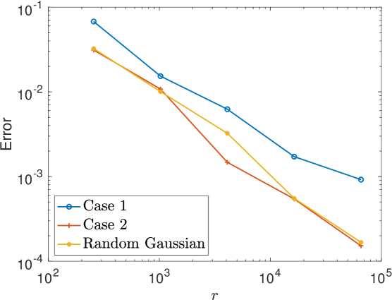
Dependence on
We set , , , and , and choose the following values for : , , , and . As shown in Figure 1, the relative error for all three strategies decreases as increases; all are of the order of . The result suggests Case-2 sketching and the Gaussian reference sketching share almost the same accuracy, while Case 1 is slightly worse.
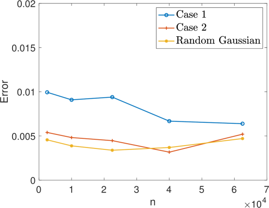
Dependence on
Theorems 3 and 4 suggest essentially no dependence on . To test this claim empirically, we fix , , and , and set to be , , , , . The error, plotted in Figure 2, shows no dependence on .
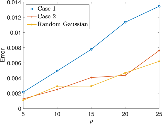
Dependence on
In this experiment, we study the dependence of relative error on . We fix , , and and let take the values , , , , . The results are plotted in Figure 3. The plot seems to indicate linear dependence on , better than the higher powers of predicted by our bounds. We leave the discussion to future research.
6.2. Electrical Impedance Tomography
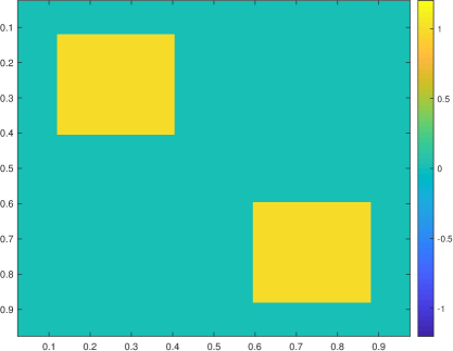
In this section, we study the EIT inverse problem on a unit square . As presented in Section 2, the goal is to reconstruct the conductivity function in (18). We assume the ground truth is an indicator function supported at the two yellow squares at the top left and bottom right corners; see Figure 4.
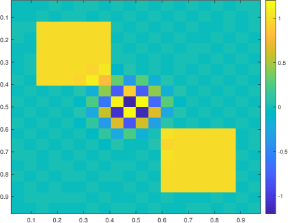
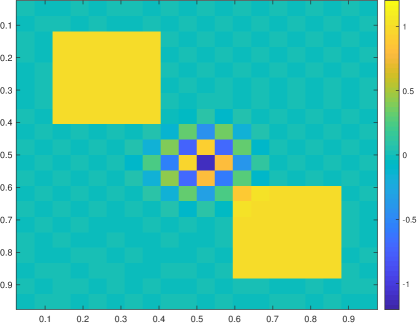
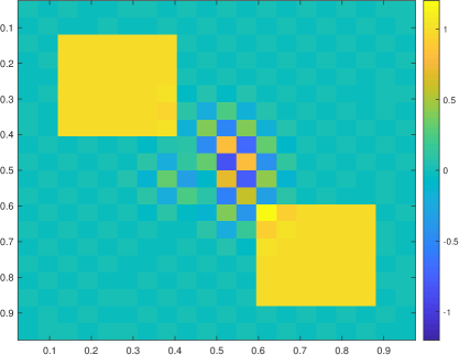
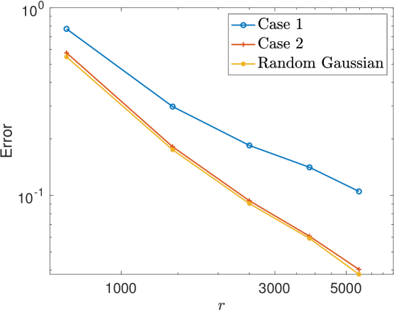
The background media (cf. (14)) is set to be a constant function with value . We use finite element method to calculate and on a uniform mesh with . The associated boundary conditions and are constructed as Dirac-delta functions at all boundary grid points. Under this setup, the matrix has dimensions . The right-hand side is generated by multiplying with the ground truth and adding white noise. The EIT inverse problem is highly ill-posed, and thus we set the standard deviation of the mean zero Gaussian noise to be small: . All three strategies are tested with different number of rows. We record the relative error (67) by taking independent trials.
In Figure 4, we plot the ground truth media and the reconstructed media using all three different strategies, with . All of them can roughly reconstruct the unknown function with some oscillatory errors in the center of the domain. In Figure 5, we plot the relative error in terms of the number of rows in the sketching matrix ( is set to be , , , , and ). We see that the Case-2 strategy performs as well as the unstructured Gaussian reference, and they both outperform Case 1.
7. Concluding remarks
Most PDE-based inverse problems, upon linearization, become Fredholm integral equations, with the testing functions being the product of two functions that are solutions to the forward and the adjoint PDEs. A Khatri-Rao matrix structure arises in the discretization. We study the sketching problem for matrices of this type, where a corresponding structure is enforced in the sketching matrix, for efficiency of computation. We construct the problem under the - embedding framework, and investigate the number of rows of the sketching matrix that are needed to reconstruct the least-squares solution with accuracy and confidence. The lower bounds differ for the two different sketching strategies that we propose, but both are independent of the size of the ambient space.
Acknowledgments
Chen, Li, and Newton are supported in part by NSF-DMS-1750488 and NSF-TRIPODS 1740707. Wright is supported in part by NSF Awards 1628384, 1634597, and 1740707; Subcontract 8F-30039 from Argonne National Laboratory; and Award N660011824020 from the DARPA Lagrange Program.
Appendix A Key Identities and Inequalities
Some identities and inequalities used repeatedly in the text are collected here.
A.1. Identities of the Kronecker product
Let , . Then the Kronecker product of and forms a matrix of size defined by:
The following properties hold.
-
(1)
Let , , and , then we have the mixed-product property:
(68) -
(2)
Let , , and . Further denote by the vectorization of formed by stacking the columns of into a single column vector, then
(69) Equivalently, given the same and , denote the matricization of the vector by aligning subvectors of that are of length into a matrix with columns, then
(70)
A.2. Sub-exponential random variables and Bernstein inequality
Properties of sub-exponential random variables used in the proofs are defined here.
Definition 3.
Sub-Exponential random variable A random variable is said to be sub-exponential with parameters (denoted as ) if and its moment generating function satisfies
| (71) |
We have the following.
Proposition 2.
Let , then is sub-exponential with parameters .
We conclude with the well known Bernstein inequality.
Proposition 3 (Bernstein inequality).
Let be i.i.d. mean zero random variables. Suppose that for all , then for any ,
| (72) |