Matrix Sketching for Secure Collaborative Machine Learning

Abstract

Collaborative learning allows participants to jointly train a model without data sharing. To update the model parameters, the central server broadcasts model parameters to the clients, and the clients send updating directions such as gradients to the server. While data do not leave a client device, the communicated gradients and parameters will leak a client’s privacy. Attacks that infer clients’ privacy from gradients and parameters have been developed by prior work. Simple defenses such as dropout and differential privacy either fail to defend the attacks or seriously hurt test accuracy. We propose a practical defense which we call Double-Blind Collaborative Learning (DBCL). The high-level idea is to apply random matrix sketching to the parameters (aka weights) and re-generate random sketching after each iteration. DBCL prevents clients from conducting gradient-based privacy inferences which are the most effective attacks. DBCL works because from the attacker’s perspective, sketching is effectively random noise that outweighs the signal. Notably, DBCL does not much increase computation and communication costs and does not hurt test accuracy at all.

1 Introduction

Collaborative learning allows multiple parties to jointly train a model using their private data but without sharing the data. Collaborative learning is motivated by real-world applications, for example, training a model using but without collecting mobile user’s data.

Distributed stochastic gradient descent (SGD) is perhaps the simplest approach to collaborative learning. Specifically, the central server broadcasts model parameters to the clients, each client uses a batch of local data to compute a stochastic gradient, and the server aggregates the stochastic gradients and updates the model parameters. Based on distributed SGD, communication-efficient algorithms such as federated averaging (FedAvg) (McMahan et al., 2017) and FedProx (Sahu et al., 2019) have been developed and analyzed (Li et al., 2019b; Stich, 2018; Wang & Joshi, 2018; Yu et al., 2019; Zhou & Cong, 2017).

Collaborative learning seemingly protects clients’ privacy. Unfortunately, this has been demonstrated not true by recent studies (Hitaj et al., 2017; Melis et al., 2019; Zhu et al., 2019). Even if a client’s data do not leave his device, important properties of his data can be disclosed from the model parameters and gradients. To infer other clients’ data, the attacker needs only to control one client device and access the model parameters in every iteration; the attacker does not have to take control of the server (Hitaj et al., 2017; Melis et al., 2019; Zhu et al., 2019).

The reason why the attacks work is that model parameters and gradients carry important information about the training data (Ateniese et al., 2015; Fredrikson et al., 2015). Hitaj et al. (2017) used the jointly learned model as a discriminator for training a generator which generates other clients’ data. Melis et al. (2019) used gradient for inferring other clients’ data properties. Zhu et al. (2019) used both model parameters and gradients for recovering other clients’ data. Judging from published empirical studies, the gradient-based attacks (Melis et al., 2019; Zhu et al., 2019) are more effective than the parameter-based attack (Hitaj et al., 2017). Our goal is to defend the gradient-based attacks.

Simple defenses, e.g., differential privacy (Dwork, 2011) and dropout (Srivastava et al., 2014), have been demonstrated not working well by (Hitaj et al., 2017; Melis et al., 2019). While differential privacy (Dwork, 2011), i.e., adding noise to model parameters or gradients, works if the noise is strong, the noise inevitably hurts the accuracy and may even stop the collaborative learning from making progress (Hitaj et al., 2017). If the noise is not strong enough, clients’ privacy will leak. Dropout training (Srivastava et al., 2014) randomly masks a fraction of the parameters, making the clients have access to only part of the parameters in each iteration. However, knowing part of the parameters is sufficient for conducting the attacks.

Proposed method.

We propose Double-Blind Collaborative Learning (DBCL) as a practical defense against gradient-based attacks, e.g., (Melis et al., 2019; Zhu et al., 2019). Technically speaking, DBCL applies random sketching (Woodruff, 2014) to the parameter matrices of a neural network, and the random sketching matrices are regenerated after each iteration. Throughout the training, the clients do not see the real model parameters; what the clients see are sketched parameters. The server does not see any real gradient or descending direction; what the server sees are approximate gradients based on sketched data and sketched parameters. This is why we call our method double-blind.

From an honest client’s perspective, DBCL is similar to dropout training, except that we use sketching to replace uniform sampling; see the discussions in Section 5.3. It is very well known that dropout does not hurt test accuracy at all (Srivastava et al., 2014; Wager et al., 2013). Since sketching has similar properties as uniform sampling, DBCL does not hurt test accuracy, which is corroborated by our empirical studies.

From an attacker’s perspective, DBCL is effectively random noise injected into the gradient, which the attacker needs for inferring other clients’ privacy. Roughly speaking, if a client tries to estimate the gradient, then he will get

$$\textrm{Estimated Grad}\;=\;\textrm{Transform }\big{(}\textrm{True Grad}\big{)}\,+\,\textrm{Noise}.\vspace{-1mm}$$

Therefore, client-side gradient-based attacks do not work. Detailed discussions are in Section 5.2.

In addition to its better security, DBCL has the following nice features:

• DBCL does not hinder test accuracy. This makes DBCL superior to the existing defenses.

• DBCL does not increase the per-iteration time complexity and communication complexity, although it reasonably increases the iterations for attaining convergence.

• When applied to dense layers and convolutional layers, DBCL does not need extra tuning.

It is worth mentioning that DBCL is not an alternative to the existing defenses; instead, DBCL can be combined with the other defenses (except dropout).

Difference from prior work.

Prior work has applied sketching to neural networks for privacy, computation, or communication benefits (Hanzely et al., 2018; Li et al., 2019a). Blocki et al. (2012); Kenthapadi et al. (2012) showed that random sketching are differential private, but the papers have very different methods and applications from our work. Hanzely et al. (2018); Li et al. (2019a) applies sketching to the gradients during federated learning. In particular, Li et al. (2019a) showed that sketching the gradients is differential private.

Our method is different from the aforementioned ones. We sketch the model parameters, not the gradients. We re-generate sketching matrices after each communication. Note that sketching the gradients protects privacy at the cost of substantial worse test accuracy. In contrast, our method does not hurt test accuracy at all.

Limitations.

While we propose DBCL as a practical defense against gradient-based attacks at little cost, we do not claim DBCL as a panacea. DBCL has two limitations. First, with DBCL applied, a malicious client cannot perform gradient-based attacks, but he may be able to perform parameter-based attacks such as (Hitaj et al., 2017); fortunately, the latter is much less effective than the former. Second, DBCL cannot prevent a malicious server from inferring clients’ privacy, although DBCL makes the server’s attack much less effective.

We admit that DBCL alone does not defeat all the attacks. To the best of our knowledge, there does not exist any defense that is effective for all the attacks that infer privacy. DBCL can be easily incorporated with existing methods such as homomorphic encryption and secret sharing to defend server-side attacks.

Paper organization.

Section 2 introduces neural network, backpropagation, and matrix sketching. Section 3 defines threat models. Section 4 describes the algorithm, including the computation and communication. Section 5 theoretically studies DBCL. Section 6 presents empirical results to demonstrate that DBCL does not harm test accuracy, does not much increase the communication cost, and can defend gradient-based attacks. Section 7 discusses related work. Algorithm derivations and theoretical proofs are in the appendix. The source code is available at the Github repo: https://github.com/MengjiaoZhang/DBCL

2 Preliminaries

Dense layer.

Let ${d_{\textrm{in}}}$ be the input shape, ${d_{\textrm{out}}}$ be the output shape, and $b$ be the batch size. Let ${\bf X}\in{\mathbb{R}}^{b\times{d_{\textrm{in}}}}$ be the input, ${\bf W}\in{\mathbb{R}}^{{d_{\textrm{out}}}\times{d_{\textrm{in}}}}$ be the parameter matrix, and ${\bf Z}={\bf X}{\bf W}^{T}$ be the output. After the dense (aka fully-connected) layer, there is typically an activation function $\sigma({\bf Z})$ applied elementwisely.

Backpropagation.

Let $L$ be the loss evaluated on a batch of $b$ training samples. We derive backpropagation for the dense layer by following the convention of PyTorch. Let ${\bf G}\triangleq\frac{\partial\,L}{\partial\,{\bf Z}}\in{\mathbb{R}}^{b\times{d_{\textrm{out}}}}$ be the gradient received from the upper layer. We need to compute the gradients:

$$\frac{\partial\,L}{\partial\,{\bf X}}\>=\>{\bf G}{\bf W}\>\in\>{\mathbb{R}}^{b\times{d_{\textrm{in}}}}\quad\textrm{and}\quad\frac{\partial\,L}{\partial\,{\bf W}}\>=\>{\bf G}^{T}{\bf X}\>\in\>{\mathbb{R}}^{{d_{\textrm{out}}}\times{d_{\textrm{in}}}},$$

which can be established by the chain rule. We use $\frac{\partial\,L}{\partial\,{\bf W}}$ to update the parameter matrix ${\bf W}$ by e.g., ${\bf W}\leftarrow{\bf W}-\eta\frac{\partial\,L}{\partial\,{\bf W}}$, and pass $\frac{\partial\,L}{\partial\,{\bf X}}$ to the lower layer.

Uniform sampling matrix.

We call ${\bf S}\in{\mathbb{R}}^{{d_{\textrm{in}}}\times s}$ a uniform sampling matrix if its columns are sampled from the set $\big{\{}\tfrac{\sqrt{{d_{\textrm{in}}}}}{\sqrt{s}}{\bf e}_{1},\cdots,\tfrac{\sqrt{{d_{\textrm{in}}}}}{\sqrt{s}}{\bf e}_{{d_{\textrm{in}}}}\big{\}}$ uniformly at random. Here, ${\bf e}_{i}$ is the $i$-th standard basis of ${\mathbb{R}}^{{d_{\textrm{in}}}}$. We call ${\bf S}$ a uniform sampling matrix because ${\bf X}{\bf S}$ contains $s$ randomly sampled (and scaled) columns of ${\bf X}$. Random matrix theories (Drineas & Mahoney, 2016; Mahoney, 2011; Martinsson & Tropp, 2020; Woodruff, 2014) guarantee that ${\mathbb{E}}_{{\bf S}}\big{[}{\bf X}{\bf S}{\bf S}^{T}{\bf W}^{T}\big{]}={\bf X}{\bf W}^{T}$ and that $\|{\bf X}{\bf S}{\bf S}^{T}{\bf W}^{T}-{\bf X}{\bf W}^{T}\|$ is bounded, for any ${\bf X}$ and ${\bf W}$.

CountSketch.

We call ${\bf S}\in{\mathbb{R}}^{{d_{\textrm{in}}}\times s}$ a CountSketch matrix (Charikar et al., 2004; Clarkson & Woodruff, 2013; Pham & Pagh, 2013; Thorup & Zhang, 2012; Weinberger et al., 2009) if it is constructed in the following way. Every row of ${\bf S}$ has exactly one nonzero entry whose position is randomly sampled from $[s]\triangleq\{1,2,\cdots,s\}$ and value is sampled from $\{-1,+1\}$. Here is an example of ${\bf S}$ ($10\times 3$):

$${\bf S}^{T}\;=\;\left[\begin{array}[]{cccccccccccccccc}0&0&1&-1&1&-1&0&0&0&0\\ -1&0&0&0&0&0&1&1&-1&0\\ 0&-1&0&0&0&0&0&0&0&1\\ \end{array}\right].$$

CountSketch has very similar properties as random Gaussian matrices (Johnson & Lindenstrauss, 1984; Woodruff, 2014). We use CountSketch for its computation efficiency. Given ${\bf X}\in{\mathbb{R}}^{b\times{d_{\textrm{in}}}}$, the CountSketch $\widetilde{{\bf X}}={\bf X}{\bf S}$ can be computed in ${\mathcal{O}}({d_{\textrm{in}}}b)$ time. CountSketch is much faster than the standard matrix multiplication which has ${\mathcal{O}}({d_{\textrm{in}}}bs)$ time complexity. Theories in (Clarkson & Woodruff, 2013; Meng & Mahoney, 2013; Nelson & Nguyên, 2013; Woodruff, 2014) guarantee that ${\mathbb{E}}_{{\bf S}}\big{[}{\bf X}{\bf S}{\bf S}^{T}{\bf W}^{T}\big{]}={\bf X}{\bf W}^{T}$ and that $\|{\bf X}{\bf S}{\bf S}^{T}{\bf W}^{T}-{\bf X}{\bf W}^{T}\|$ is bounded, for any ${\bf X}$ and ${\bf W}$. In practice, ${\bf S}$ is not explicitly constructed.

3 Threat Models

In this paper, we consider attacks and defenses under the setting of client-server architecture; we assume the attacker controls a client. Let ${\bf W}_{\textrm{old}}$ and ${\bf W}_{\textrm{new}}$ be the model parameters (aka weights) in two consecutive iterations. The server broadcasts ${\bf W}_{\textrm{old}}$ to the clients, the $m$ clients use ${\bf W}_{\textrm{old}}$ and their local data to compute ascending directions ${\boldsymbol{\Delta}}_{1},\cdots,{\boldsymbol{\Delta}}_{m}$ (e.g., gradients), and the server aggregates the directions by ${\boldsymbol{\Delta}}=\frac{1}{m}\sum_{i=1}^{m}{\boldsymbol{\Delta}}_{i}$ and performs the update ${\bf W}_{\textrm{new}}\leftarrow{\bf W}_{\textrm{old}}-{\boldsymbol{\Delta}}$. Since a client (say the $k$-th) knows ${\bf W}_{\textrm{old}}$, ${\bf W}_{\textrm{new}}$, and his own direction ${\boldsymbol{\Delta}}_{k}$, he can calculate the sum of other clients’ directions by

$$\sum_{i\neq k}{\boldsymbol{\Delta}}_{i} = m{\boldsymbol{\Delta}}-{\boldsymbol{\Delta}}_{k}$$ (1)

$$= m\big{(}{\bf W}_{\textrm{old}}-{\bf W}_{\textrm{new}}\big{)}-{\boldsymbol{\Delta}}_{k}.$$

In the case of two-party collaborative learning, that is, $m=2$, one client knows the updating direction of the other client.

Knowing the model parameters, gradients, or both, the attacker can use various ways (Hitaj et al., 2017; Melis et al., 2019; Zhu et al., 2019) to infer other clients’ privacy. We focus on gradient-based attacks (Melis et al., 2019; Zhu et al., 2019), that is, the victim’s privacy is extracted from the gradients. Melis et al. (2019) (Melis et al., 2019) built a classifier and locally trained it for property inference. The classifier takes the updating direction ${\boldsymbol{\Delta}}_{i}$ as input feature and predicts the clients’ data properties. The client’s data cannot be recovered, however, the classifier can tell, e.g., the photo is likely female. Zhu et al. (2019) (Zhu et al., 2019) developed an optimization method called gradient matching for recovering other clients’ data; both gradient and model parameters are used. It has been shown that simple defenses such as differential privacy (Dwork & Naor, 2010; Dwork, 2011) and dropout (Srivastava & Nedic, 2011) cannot defend the attacks.

In decentralized learning, where participants are compute nodes in a peer-to-peer network, a node knows its neighbors’ model parameters and thereby updating directions. A node can infer the privacy of its neighbors in the same way as (Melis et al., 2019; Zhu et al., 2019). In Appendix D, we discuss the attack and defense in decentralized learning; they will be our future work.

4 Proposed Method

We present the high-level ideas in Section 4.1, elaborate on the implementation in Section 4.2, and analyze the time and communication complexities in Section 4.3.

4.1 High-Level Ideas

The attacks of (Melis et al., 2019; Zhu et al., 2019) need the victim’s updating direction, e.g., gradient, for inferring the victim’s privacy. Using standard distributed algorithms such as distributed SGD and Federated Averaging (FedAvg) (McMahan et al., 2017), the server can see the clients’ updating directions, ${\boldsymbol{\Delta}}_{1},\cdots,{\boldsymbol{\Delta}}_{m}$, and the clients can see the jointly learned model parameter, ${\bf W}$. A malicious client can use (1) to get other clients’ updating directions and then perform the gradient-based attacks such as (Melis et al., 2019; Zhu et al., 2019).

To defend the gradient-based attacks, our proposed Double-Blind Collaborative Learning (DBCL) applies random sketching to the inputs and parameter matrices. Let ${\bf X}$ and ${\bf W}$ be the input batch and parameter matrix of a dense layer, respectively. For some or all the dense layers, replace ${\bf X}$ and ${\bf W}$ by $\widetilde{{\bf X}}={\bf X}{\bf S}$ and $\widetilde{{\bf W}}={\bf W}{\bf S}$, respectively, and different layers have different sketching matrices, ${\bf S}$. Each time ${\bf W}$ is updated, we re-generate ${\bf S}$. DBCL is applicable to convolutional layers in a similar way; see Appendix B.2.

Let ${\bf W}_{\textrm{old}}$ and ${\bf W}_{\textrm{new}}$ be the true parameter matrices in two consecutive iterations; they are known to only the server. The clients do not observe ${\bf W}_{\textrm{old}}$ and ${\bf W}_{\textrm{new}}$. What the clients observe are the random sketches: $\widetilde{{\bf W}}_{\textrm{old}}={\bf W}_{\textrm{old}}{\bf S}_{\textrm{old}}$ and $\widetilde{{\bf W}}_{\textrm{new}}={\bf W}_{\textrm{new}}{\bf S}_{\textrm{new}}$. In addition, the clients know ${\bf S}_{\textrm{old}}$ and ${\bf S}_{\textrm{new}}$. To perform gradient-based attacks, a client seeks to estimate ${\boldsymbol{\Delta}}={\bf W}_{\textrm{old}}-{\bf W}_{\textrm{new}}$ based on what it knows, i.e., $\widetilde{{\bf W}}_{\textrm{old}}$, $\widetilde{{\bf W}}_{\textrm{new}}$, ${\bf S}_{\textrm{old}}$ and ${\bf S}_{\textrm{new}}$. Our theories and experiments show that a client’s estimate of ${\boldsymbol{\Delta}}$ is far from the truth.

4.2 Algorithm Description

We describe the computation and communication operations of DBCL. We consider the client-server architecture, dense layers, and the distributed SGD algorithm. DBCL works in the following four steps. Broadcasting and aggregation are communication operations; forward pass and backward pass are local computations performed by each client for calculating gradients.

Broadcasting.

The central server generates a new seed $\psi$ and then a random sketch: $\widetilde{{\bf W}}={\bf W}{\bf S}$. It broadcasts $\psi$ and $\widetilde{{\bf W}}\in{\mathbb{R}}^{{d_{\textrm{out}}}\times s}$ to all the clients through message passing. Here, the sketch size $s$ is determined by the server and must be set smaller than ${d_{\textrm{in}}}$; the server may vary $s$ after each iteration.

Local forward pass.

The $i$-th client randomly selects a batch of $b$ samples from its local dataset and then locally performs a forward pass. Let the input of a dense layer be ${\bf X}_{i}\in{\mathbb{R}}^{b\times{d_{\textrm{in}}}}$. The client uses the seed $\psi$ to draw a sketch $\widetilde{{\bf X}}_{i}={\bf X}_{i}{\bf S}\in{\mathbb{R}}^{b\times s}$ and computes ${\bf Z}_{i}=\widetilde{{\bf X}}_{i}\widetilde{{\bf W}}^{T}$. Then $\sigma({\bf Z}_{i})$ becomes the input of the upper layer, where $\sigma$ is some activation function. Repeat this process for all the layers. The forward pass finally outputs $L_{i}$, the loss evaluated on the batch of $b$ samples.

Local backward pass.

Let the local gradient propagated to the dense layer be ${\bf G}_{i}\triangleq\frac{\partial\,L_{i}}{\partial\,{\bf Z}_{i}}\in{\mathbb{R}}^{b\times{d_{\textrm{out}}}}$. The client locally calculates

$$\mbox{\boldmath$\Gamma$\unboldmath}_{i}\>=\>{\bf G}_{i}^{T}\widetilde{{\bf X}}_{i}\>\in\>{\mathbb{R}}^{{d_{\textrm{out}}}\times s}\;\;\textrm{and}\;\;\frac{\partial\,L_{i}}{\partial\,{\bf X}_{i}}\>=\>{\bf G}_{i}\widetilde{{\bf W}}{\bf S}^{T}\>\in\>{\mathbb{R}}^{b\times{d_{\textrm{in}}}}.$$

The gradient $\frac{\partial\,L_{i}}{\partial\,{\bf X}_{i}}$ is propagated to the lower-level layer to continue the backpropagation.

Aggregation.

The server aggregates $\{\mbox{\boldmath$\Gamma$\unboldmath}_{i}\}_{i=1}^{m}$ to compute $\mbox{\boldmath$\Gamma$\unboldmath}=\frac{1}{m}\sum_{i=1}^{m}\mbox{\boldmath$\Gamma$\unboldmath}_{i}$; this needs a communication. Let $L=\frac{1}{m}\sum_{i=1}^{m}L_{i}$ be the loss evaluated on the batch of $mb$ samples. It can be shown that

$$\frac{\partial\,L}{\partial\,{\bf W}}\>=\>\frac{1}{m}\sum_{i=1}^{m}\frac{\partial\,L_{i}}{\partial\,{\bf W}}\>=\>\mbox{\boldmath$\Gamma$\unboldmath}{\bf S}^{T}\>\in\>{\mathbb{R}}^{{d_{\textrm{out}}}\times{d_{\textrm{in}}}}.$$ (2)

The server then updates the parameters by, e.g., ${\bf W}\leftarrow{\bf W}-\eta\frac{\partial\,L}{\partial\,{\bf W}}$.

4.3 Time Complexity and Communication Complexity

DBCL does not increase the time complexity of local computations. The CountSketch, $\widetilde{{\bf X}}_{i}={\bf X}_{i}{\bf S}$ and $\widetilde{{\bf W}}_{i}={\bf W}_{i}{\bf S}$, costs ${\mathcal{O}}(b{d_{\textrm{in}}})$ and ${\mathcal{O}}({d_{\textrm{in}}}{d_{\textrm{out}}})$ time, respectively. Using CountSketch, the overall time complexity of a forward and a backward pass is ${\mathcal{O}}(b{d_{\textrm{in}}}+{d_{\textrm{in}}}{d_{\textrm{out}}}+bs{d_{\textrm{out}}})$. Since we set $s<{d_{\textrm{in}}}$ to protect privacy, the time complexity is lower than the standard backpropagation, ${\mathcal{O}}(b{d_{\textrm{in}}}{d_{\textrm{out}}})$.

DBCL does not increase per-iteration communication complexity. Without using sketching, the communicated matrices are ${\bf W}\in{\mathbb{R}}^{{d_{\textrm{out}}}\times{d_{\textrm{in}}}}$ and $\frac{\partial\,L_{i}}{\partial\,{\bf W}}\in{\mathbb{R}}^{{d_{\textrm{out}}}\times{d_{\textrm{in}}}}$. Using sketching, the communicated matrices are $\widetilde{{\bf W}}\in{\mathbb{R}}^{{d_{\textrm{out}}}\times s}$ and $\mbox{\boldmath$\Gamma$\unboldmath}_{i}\in{\mathbb{R}}^{{d_{\textrm{out}}}\times s}$. Because $s<{d_{\textrm{in}}}$, the per-iteration communication complexity is lower than the standard distributed SGD.

5 Theoretical Insights

In Section 5.1, we discuss how a malicious client makes use of the sketched model parameters for privacy inference. In Sections 5.2, we show that DBCL can defend certain types of attacks. In Section 5.3, we give an explanation of DBCL from optimization perspective.

5.1 Approximating the Gradient

Assume the attacker controls a client and participates in collaborative learning. Let ${\bf W}_{\textrm{old}}$ and ${\bf W}_{\textrm{new}}$ be the parameter matrices of two consecutive iterations; they are unknown to the clients. What a client sees are the sketches, $\widetilde{{\bf W}}_{\textrm{old}}={\bf W}_{\textrm{old}}{\bf S}_{\textrm{old}}$ and $\widetilde{{\bf W}}_{\textrm{new}}={\bf W}_{\textrm{new}}{\bf S}_{\textrm{new}}$. To conduct gradient-based attacks, the attacker must know the gradient ${\boldsymbol{\Delta}}={\bf W}_{\textrm{old}}-{\bf W}_{\textrm{new}}$.

Without using ${\bf S}_{\textrm{old}}$ and ${\bf S}_{\textrm{new}}$, one cannot recover ${\boldsymbol{\Delta}}$, not even approximately. The difference between sketched parameters, $\widetilde{{\boldsymbol{\Delta}}}=\widetilde{{\bf W}}_{\textrm{old}}-\widetilde{{\bf W}}_{\textrm{new}}$, is entirely different from the real gradient, ${{\boldsymbol{\Delta}}}={{\bf W}}_{\textrm{old}}-{{\bf W}}_{\textrm{new}}$. We can even vary the sketch size $s$ with iterations so that $\widetilde{{\bf W}}_{\textrm{old}}$ and $\widetilde{{\bf W}}_{\textrm{new}}$ have different number of columns, making it impossible to compute ${{\bf W}}_{\textrm{old}}-{{\bf W}}_{\textrm{new}}$.

Note that the clients know also ${\bf S}_{\textrm{old}}$ and ${\bf S}_{\textrm{new}}$. A smart attacker, who knows random matrix theory, may want to use

$$\widehat{{\boldsymbol{\Delta}}}={\bf W}_{\textrm{old}}{\bf S}_{\textrm{old}}{\bf S}_{\textrm{old}}^{T}-{\bf W}_{\textrm{new}}{\bf S}_{\textrm{new}}{\bf S}_{\textrm{new}}^{T}$$

to approximate ${\boldsymbol{\Delta}}$. It is because $\widehat{{\boldsymbol{\Delta}}}$ is an unbiased estimate of ${\boldsymbol{\Delta}}$, i.e., ${\mathbb{E}}\big{[}\widehat{{\boldsymbol{\Delta}}}\big{]}={\boldsymbol{\Delta}}$, where the expectation is taken w.r.t. the random sketching matrices ${\bf S}_{\textrm{old}}$ and ${\bf S}_{\textrm{new}}$.

5.2 Defending Gradient-Based Attacks

We analyze the attack that uses $\widehat{{\boldsymbol{\Delta}}}$. We first give an intuitive explanation and then prove that using $\widehat{{\boldsymbol{\Delta}}}$ does not work, unless the magnitude of ${\boldsymbol{\Delta}}$ is smaller than ${\bf W}_{\textrm{new}}$.

Matrix sketching as implicit noise.

As $\widehat{{\boldsymbol{\Delta}}}$ is an unbiased estimate of ${\boldsymbol{\Delta}}$, the reader may wonder why $\widehat{{\boldsymbol{\Delta}}}$ does not disclose the information of ${\boldsymbol{\Delta}}$. Here we give an intuitive explanation. $\widehat{{\boldsymbol{\Delta}}}$ is a mix of ${\boldsymbol{\Delta}}$ (which is the signal) and a random transformation of ${\bf W}_{\textrm{new}}$ (which is random noise):

$$\widehat{{\boldsymbol{\Delta}}}\>=\>\underbrace{{\boldsymbol{\Delta}}}_{\textrm{signal}}{\bf S}_{\textrm{old}}{\bf S}_{\textrm{old}}^{T}+\underbrace{{\bf W}_{\textrm{new}}\big{(}{\bf S}_{\textrm{old}}{\bf S}_{\textrm{old}}^{T}-{\bf S}_{\textrm{new}}{\bf S}_{\textrm{new}}^{T}\big{)}}_{\textrm{zero-mean noise}}.$$ (3)

As the magnitude of ${\bf W}$ is much greater than ${\boldsymbol{\Delta}}$, the noise outweighs the signal, making $\widehat{{\boldsymbol{\Delta}}}$ far from ${\boldsymbol{\Delta}}$. From the attacker’s perspective, random sketching is effectively random noise that outweighs the signal.

Defending the gradient matching attack of (Zhu et al., 2019).

The gradient matching attack can recover the victim’s original data based on the victim’s gradient, ${\boldsymbol{\Delta}}_{i}$, and the model parameters, ${\bf W}$. Numerical optimization is used to find the data on which the computed gradient matches ${\boldsymbol{\Delta}}_{i}$. To get ${\boldsymbol{\Delta}}_{i}$, the attacker must know ${\boldsymbol{\Delta}}=\sum_{i=1}^{m}{\boldsymbol{\Delta}}_{i}$. Using DBCL, no client knows ${\boldsymbol{\Delta}}$. A smart attacker may want to use $\widehat{{\boldsymbol{\Delta}}}$ in lieu of ${\boldsymbol{\Delta}}$ because of its unbiasedness. We show in Theorem 1 that this approach does not work.

Theorem 1.

Let ${\bf S}_{\textrm{old}}$ and ${\bf S}_{\textrm{new}}$ be ${{d_{\textrm{in}}}\times s}$ CountSketch matrices and $s<{d_{\textrm{in}}}$. Then

$${\mathbb{E}}\big{\|}\widehat{{\boldsymbol{\Delta}}}-{\boldsymbol{\Delta}}\big{\|}_{F}^{2}\>=\>\Omega\Big{(}\frac{{d_{\textrm{in}}}}{s}\Big{)}\cdot\Big{(}\big{\|}{\bf W}_{\textrm{old}}\big{\|}_{F}^{2}+\big{\|}{\bf W}_{\textrm{new}}\big{\|}_{F}^{2}\Big{)}.$$

Since the magnitude of ${\boldsymbol{\Delta}}$ is typically smaller than ${\bf W}$, Theorem 1 guarantees that using $\widehat{{\boldsymbol{\Delta}}}$ is no better than all-zeros or random guessing.

Remark 1.

The theorem shows that DBCL beats one way of gradient estimate. Admittedly, the theorem does not guarantee that DBCL can defend all kinds of gradient estimates. A stronger bound would be:

$$\min_{{\bf Z}_{1},{\bf Z}_{2}}\left\|{\bf W}_{\textrm{old}}{\bf S}_{\textrm{old}}{\bf Z}_{1}-{\bf W}_{\textrm{new}}{\bf S}_{\textrm{new}}{\bf Z}_{2}-{\boldsymbol{\Delta}}\right\|_{F}^{2}=\Omega(1)\cdot\big{\|}{\boldsymbol{\Delta}}\big{\|}_{F}^{2}.$$

Unfortunately, at this time, we do not know how to prove such a bound.

Defending the property inference attack (PIA) of (Melis et al., 2019).

To conduct the PIA of (Melis et al., 2019), the attacker may want to use a linear model parameterized by ${\bf V}$. According to (1), the attacker uses ${\boldsymbol{\Delta}}-{\bf A}$ as input features for PIA, where ${\bf A}$ is some fixed matrix known to the attacker. The linear model makes prediction by ${\bf Y}\triangleq({\boldsymbol{\Delta}}-{\bf A}){\bf V}^{T}$. Using $\widehat{{\boldsymbol{\Delta}}}$ to approximate ${\boldsymbol{\Delta}}$, the prediction is $\widehat{{\bf Y}}\triangleq(\widehat{{\boldsymbol{\Delta}}}-{\bf A}){\bf V}^{T}$. Theorem 2 and Corollary 3 show that $\|\widehat{{\bf Y}}-{\bf Y}\|_{F}^{2}=\|\widehat{{\boldsymbol{\Delta}}}{\bf V}^{T}-{\boldsymbol{\Delta}}{\bf V}^{T}\|_{F}^{2}$ is very big.

Theorem 2.

Let ${\bf S}_{\textrm{old}}$ and ${\bf S}_{\textrm{new}}$ be ${{d_{\textrm{in}}}\times s}$ CountSketch matrices and $s<{d_{\textrm{in}}}$. Let $w_{pq}$ be the $(p,q)$-th entry of ${\bf W}_{\textrm{old}}\in{\mathbb{R}}^{{d_{\textrm{out}}}\times{d_{\textrm{in}}}}$ and $\tilde{w}_{pq}$ be the $(p,q)$-th entry of ${\bf W}_{\textrm{new}}\in{\mathbb{R}}^{{d_{\textrm{out}}}\times{d_{\textrm{in}}}}$. Let ${\bf V}$ be any $r\times{d_{\textrm{in}}}$ matrix and $v_{pq}$ be the $(p,q)$-th entry of ${\bf V}$. Then

$${\mathbb{E}}\big{\|}\widehat{{\boldsymbol{\Delta}}}{\bf V}^{T}-{\boldsymbol{\Delta}}{\bf V}^{T}\big{\|}_{F}^{2}\;=\>\frac{1}{s}\sum_{i=1}^{{d_{\textrm{out}}}}\sum_{j=1}^{r}\sum_{k\neq l}$$

$$\qquad\quad\bigg{(}w_{ik}^{2}v_{jl}^{2}+w_{ik}v_{jk}w_{il}v_{jl}+\tilde{w}_{ik}^{2}v_{jl}^{2}+\tilde{w}_{ik}v_{jk}\tilde{w}_{il}v_{jl}\bigg{)}.$$

The bound in Theorem 2 is involved. To interpret the bound, we add (somehow unrealistic) assumptions and obtain Corollary 3.

Corollary 3.

Let ${\bf S}$ be a ${{d_{\textrm{in}}}\times s}$ CountSketch matrix and $s<{d_{\textrm{in}}}$. Assume that the entries of ${\bf W}_{\textrm{old}}$ are IID and that the entries of ${\bf V}$ are also IID. Then

$${\mathbb{E}}\big{\|}\widehat{{\boldsymbol{\Delta}}}{\bf V}^{T}-{\boldsymbol{\Delta}}{\bf V}^{T}\big{\|}_{F}^{2}\>=\>\Omega\Big{(}\frac{{d_{\textrm{in}}}}{s}\Big{)}\cdot\big{\|}{\bf W}_{\textrm{old}}{\bf V}^{T}\big{\|}_{F}^{2}.$$

Since the magnitude of ${\boldsymbol{\Delta}}$ is much smaller than ${\bf W}$, especially when ${\bf W}$ is close to a stationary point, $\|{\bf W}{\bf V}^{T}\|_{F}^{2}$ is typically greater than $\|{\boldsymbol{\Delta}}{\bf V}^{T}\|_{F}^{2}$. Thus, ${\mathbb{E}}\|\widehat{{\boldsymbol{\Delta}}}{\bf V}^{T}-{\boldsymbol{\Delta}}{\bf V}^{T}\|_{F}^{2}$ is typically bigger than $\|{\boldsymbol{\Delta}}{\bf V}^{T}\|_{F}^{2}$, which implies that using $\widehat{{\boldsymbol{\Delta}}}$ is no better than all-zeros or random guessing.

Table 1: Experiments on MNIST. The table shows the rounds of communications for attaining the test accuracy. Here, $c$ is the participation ratio of FedAvg, that is, in each round, only a fraction of clients participate in the training.

Models	Accuracy	Communication Rounds
		$c=1\%$	$c=10\%$	$c=20\%$	$c=50\%$	$c=100\%$
MLP	$0.97$	222	96	84	83	82
MLP-Sketch	$0.97$	572	322	308	298	287
CNN	$0.99$	462	309	97	91	31
CNN-Sketch	$0.99$	636	176	189	170	174

5.3 Understanding DBCL from Optimization Perspective

We give an explanation of DBCL from optimization perspective. Let us consider the generalized linear model:

$$\mathop{\rm argmin}_{{\bf w}}\;\bigg{\{}{f}({\bf w})\>\triangleq\>\frac{1}{n}\sum_{j=1}^{n}\ell\big{(}{\bf x}_{i}^{T}{\bf w},\,y_{j}\big{)}\bigg{\}},$$ (4)

where $({\bf x}_{1},y_{1}),\cdots,({\bf x}_{n},y_{n})$ are the training samples and $\ell(\cdot,\cdot)$ is the loss function. If we apply sketching to a generalized linear model, then the training will be solving the following problem:

$$\mathop{\rm argmin}_{{\bf w}}\;\bigg{\{}\tilde{f}({\bf w})\>\triangleq\>{\mathbb{E}}_{{\bf S}}\bigg{[}\frac{1}{n}\sum_{j=1}^{n}\ell\big{(}{\bf x}_{i}^{T}{\bf S}{\bf S}^{T}{\bf w},\,y_{j}\big{)}\bigg{]}\bigg{\}}.$$ (5)

Note that (5) is different from (4). If ${\bf S}$ is a uniform sampling matrix, then (5) will be empirical risk minimization with dropout. Prior work (Wager et al., 2013) proved that dropout is equivalent to adaptive regularization which can alleviate overfitting. Random projections such as CountSketch have the same properties as uniform sampling (Woodruff, 2014), and thus the role of random sketching in (5) can be thought of as adaptive regularization. This is why DBCL does not hinder prediction accuracy at all.

6 Experiments

We conduct experiments to demonstrate that first, DBCL does not harm test accuracy, second, DBCL does not increase the communication cost too much, and third, DBCL can defend client-side gradient-based attacks.

6.1 Experiment Setting

Our method and the compared methods are implemented using PyTorch. The experiments are conducted on a server with 4 NVIDIA GeForce Titan V GPUs, 2 Xeon Gold 6134 CPUs, and 192 GB memory. We follow the settings of the relevant papers to perform comparisons.

Three datasets are used in the experiments. MNIST has 60,000 training images and 10,000 test images; each image is $28\times 28$. CIFAR-10 has 50,000 training images and 10,000 test images; each image is $32\times 32\times 3$. Labeled Faces In the Wild (LFW) has 13,233 faces of 5,749 individuals; each face is a $64\times 47\times 3$ color image.

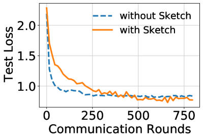
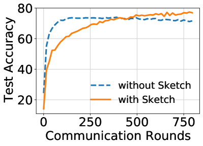
(a) Test loss. (b) Test Accuracy. Figure 1: Experiment on CIFAR-10 dataset. The test accuracy do not match the state-of-the-art because the CNN is small and we do not use advanced tricks; we follow the settings of the seminal work (McMahan et al., 2017).          Figure 2: Gender classification on the LWF dataset.

6.2 Accuracy and Efficiency

We conduct experiments on the MNIST and CIFAR-10 datasets to show that first, DBCL does not hinder prediction accuracy, and second, it does not much increase the communication cost. We follow the setting of (McMahan et al., 2017). The learning rates are tuned to optimize the convergence rate.

MNIST classification.

We build a multilayer perceptron (MLP) and a convolutional neural network (CNN) for the multi-class classification task. The MLP has 3 dense layers: $\textsf{Dense}(200)$ $\Rightarrow$ ReLU $\Rightarrow$ $\textsf{Dense}(200)$ $\Rightarrow$ ReLU $\Rightarrow$ $\textsf{Dense}(10)$ $\Rightarrow$ Softmax. The CNN has 2 convolutional layers and 2 dense layers: $\textsf{Conv}(32,5\times 5)$ $\Rightarrow$ ReLU $\Rightarrow$ $\textsf{MaxPool}(2\times 2)$ $\Rightarrow$ $\textsf{Conv}(64,5\times 5)$ $\Rightarrow$ ReLU $\Rightarrow$ $\textsf{MaxPool}(2\times 2)$ $\Rightarrow$ Flatten $\Rightarrow$ $\textsf{Dense}(512)$ $\Rightarrow$ ReLU $\Rightarrow$ $\textsf{Dense}(10)$ $\Rightarrow$ Softmax.

We use Federated Averaging (FedAvg) to train the MLP and CNN. The data are partitioned among $100$ (virtual) clients uniformly at random. Between two communications, FedAvg performs local computation for 1 epoch (for MLP) or 5 epochs (for CNN). The batch size of local SGD is set to $10$.

Sketching is applied to all the dense and convolutional layers except the output layer. We set the sketch size to $s={d_{\textrm{in}}}/2$; thus, the per-communication word complexity is reduced by half. With sketching, the MLP and CNN are trained by FedAvg under the same setting.

We show the experimental results in Table 1. Trained by FedAvg, the small MLP can only reach 97% test accuracy, while the CNN can obtain 99% test accuracy. In this set of experiments, sketching does not hinder test accuracy at all. We show the rounds of communications for attaining the test accuracies. For the MLP, sketching needs 2.6x $\sim$ 3.6x rounds of communications to converge. For the CNN, sketching needs 0.6x $\sim$ 5.6x rounds of communications to converge. Using sketching, the per-communication word complexity is reduced to 0.5x.

CIFAR-10 classification.

We build a CNN with 3 convolutional layers and 2 dense layers: $\textsf{Conv}(32,5\times 5)$ $\Rightarrow$ ReLU $\Rightarrow$ $\textsf{Conv}(64,5\times 5)$ $\Rightarrow$ ReLU $\Rightarrow$ $\textsf{MaxPool}(2\times 2)$ $\Rightarrow$ $\textsf{Conv}(128,5\times 5)$ $\Rightarrow$ ReLU $\Rightarrow$ $\textsf{MaxPool}(2\times 2)$ $\Rightarrow$ Flatten $\Rightarrow$ $\textsf{Dense}(200)$ $\Rightarrow$ ReLU $\Rightarrow$ $\textsf{Dense}(10)$ $\Rightarrow$ Softmax.

The CNN is also trained using FedAvg. The data are partitioned among $100$ clients. We set the participation ratio to $c=10\%$, that is, each time only $10\%$ uniformly sampled clients participate in the training. Between two communications, FedAvg performs local computation for 5 epochs. The batch size of local SGD is set to $50$. We follow the settings of (McMahan et al., 2017), so we do not use tricks such as data augmentation, batch normalization, skip connection, etc.

Figure 2 shows the convergence curves. Using sketching does not hinder the test accuracy at all; on the contrary, it marginally improves the test accuracy. The reason is likely that sketching is an adaptive regularization similar to dropout; see the discussions in Section 5.3.

Binary classification on imbalanced data.

Following (Melis et al., 2019), we conduct binary classification experiments on a subset of the LFW dataset. We use $8,150$ faces for training and $3,400$ for test. The task is gender prediction. We build a CNN with 3 convolutional layers and 3 dense layers: $\textsf{Conv}(64,3\times 3)$ $\Rightarrow$ ReLU $\Rightarrow$ $\textsf{MaxPool}(2\times 2)$ $\Rightarrow$ $\textsf{Conv}(64,3\times 3)$ $\Rightarrow$ ReLU $\Rightarrow$ $\textsf{MaxPool}(2\times 2)$ $\Rightarrow$ $\textsf{Conv}(128,3\times 3)$ $\Rightarrow$ ReLU $\Rightarrow$ $\textsf{MaxPool}(2\times 2)$ $\Rightarrow$ Flatten $\Rightarrow$ $\textsf{Dense}(32)$ $\Rightarrow$ ReLU $\Rightarrow$ $\textsf{Dense}(32)$ $\Rightarrow$ ReLU $\Rightarrow$ $\textsf{Dense}(1)$ $\Rightarrow$ Sigmoid. We apply sketching to all the convolutional and dense layers except the output layer. The model is trained by distributed SGD (2 clients and 1 server) with a learning rate of $0.01$ and a batch size of $32$.

The dataset is class-imbalanced: 8957 are males, and 2593 are females. We therefore use ROC curves, instead of classification accuracy, for evaluating the classification. In Figure 2, we plot the ROC curves to compare the standard CNN and the sketched one. The two ROC curves are almost the same.

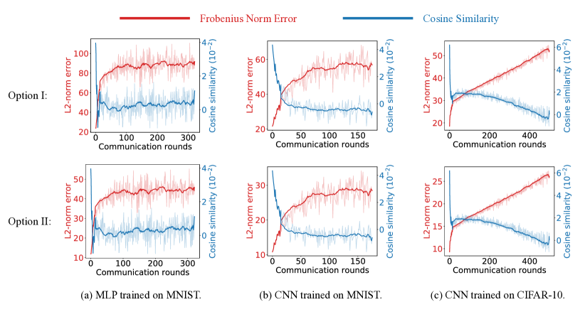
Figure 3: The x-axis is the communication rounds. The y-axes are Frobenius norm errors (red) and cosine similarities (blue). The figures show that the estimated gradient, $\widehat{{\boldsymbol{\Delta}}}$, is far from the true gradient, ${\boldsymbol{\Delta}}$, which means our defense works.

6.3 Defending Gradient-Based Attacks

We empirically study whether DBCL can defend the gradient-based attacks of (Melis et al., 2019) and (Zhu et al., 2019). The details of experiment setting are in the appendix.

Gradient estimation.

To perform gradient-based attacks, a client needs to (approximately) know the gradient (or other updating directions). We discuss in Section 5.1 how a client can estimate the updating directions. We empirically study two approaches:

Option I: $$\widehat{{\boldsymbol{\Delta}}}={\bf W}_{\textrm{old}}{\bf S}_{\textrm{old}}{\bf S}_{\textrm{old}}^{T}-{\bf W}_{\textrm{new}}{\bf S}_{\textrm{new}}{\bf S}_{\textrm{new}}^{T},$$

Option II: $$\widehat{{\boldsymbol{\Delta}}}={\bf W}_{\textrm{old}}{\bf S}_{\textrm{old}}{\bf S}_{\textrm{old}}^{\dagger}-{\bf W}_{\textrm{new}}{\bf S}_{\textrm{new}}{\bf S}_{\textrm{new}}^{\dagger}.$$

Here, ${\bf A}^{\dagger}$ means the Moore-Penrose inverse of matrix ${\bf A}$. Let ${\boldsymbol{\Delta}}={\bf W}_{\textrm{old}}-{\bf W}_{\textrm{new}}$ be the true updating direction. We evaluate the approximation quality using two metrics:

The $$\ell_{2} \big{\|}\mathrm{vec}\big{(}\widehat{{\boldsymbol{\Delta}}}-{\boldsymbol{\Delta}}\big{)}\big{\|}_{2}\,\big{/}\,\big{\|}\mathrm{vec}\big{(}{\boldsymbol{\Delta}}\big{)}\big{\|}_{2},$$-norm error:

Cosine similarity: $$\big{\langle}\,\mathrm{vec}\big{(}\widehat{{\boldsymbol{\Delta}}}\big{)}\,,\,\mathrm{vec}\big{(}{\boldsymbol{\Delta}}\big{)}\,\big{\rangle}.$$

If $\widehat{{\boldsymbol{\Delta}}}$ is far from ${\boldsymbol{\Delta}}$, which means our defense is effective, then the $\ell_{2}$ error is big, and the cosine similarity is small.

Figure 3 plots the quality of gradient estimation. The experiment settings are the same as Section 6.2; the participation ratio is set to $10\%$. The results show that $\widehat{{\boldsymbol{\Delta}}}$ is entirely different from ${\boldsymbol{\Delta}}$, which means our defense works. Equation (3) implies that as the magnitude of ${\boldsymbol{\Delta}}$ decreases, $\widehat{{\boldsymbol{\Delta}}}$ is dominated by noise, and thus the error $\frac{\|\mathrm{vec}(\widehat{{\boldsymbol{\Delta}}}-{\boldsymbol{\Delta}})\|_{2}}{\|\mathrm{vec}({\boldsymbol{\Delta}})\|_{2}}$ gets bigger. In our experiments, as the communication rounds increase, the algorithm tends to converge, the magnitude of ${\boldsymbol{\Delta}}$ decreases, and the error increases. The empirical observations verify our theories.

Defending the property inference attack (PIA) of Melis et al. (2019).

We conduct experiments on the LFW dataset. The task of collaborative learning is the gender classification under the same setting as Section 6.2. The attacker seeks to infer whether a single batch of photos in the victim’s private dataset contain Africans or not. We use one server and two clients, which is the easiest for the attacker.

• Let one client be the attacker and the other client be the victim. Without sketching, the AUC is 1.0, which means the attacker is always right. With sketching applied, the AUC is 0.5, which means the performance is the same as random guess.

• Let the server be the attacker and one client be the victim. Without sketching, the AUC is 1.0, which means the attacker succeeds. With sketching applied, the AUC is $0.726$. Our defense makes server-side attack much less effective, but users’ privacy can still leak.

Defending the gradient-matching attack of Zhu et al. (2019).

The attack seeks to recover the victims’ data using model parameters and gradients. They seek to find a batch of images by optimization so that the resulting gradient matches the observed gradient of the victim. We use the same CNNs as (Zhu et al., 2019) to conduct experiments on the MNIST and CIFAR-10 datasets. Without using sketching, the gradient-matching attack very well recovers the images. For both client-side attacks and server-side attacks, if sketching is applied to all except the output layer, then the recovered images are just like random noise. The experiments show that we can defend gradient-matching attack performed by both server and client.

7 Related Work

Cryptography approaches such as secure aggregation (Bonawitz et al., 2017), homomorphic encryption (Aono et al., 2017; Giacomelli et al., 2018; Gilad-Bachrach et al., 2016; Liu et al., 2018; Zhang et al., 2018b), Yao’s garbled circuit protocol (Rouhani et al., 2018), and many other methods (Yuan & Yu, 2013; Zhang et al., 2018a) can also improve the security of collaborative learning. Generative models such as (Chen et al., 2018) can also improve privacy; however, they hinder the accuracy and efficiency, and their tuning and deployment are nontrivial. All the mentioned defenses are not competitive methods of our DBCL; instead, they can be combined with DBCL to defend more attacks.

Our methodology is based on matrix sketching (Johnson & Lindenstrauss, 1984; Drineas et al., 2008; Halko et al., 2011; Mahoney, 2011; Woodruff, 2014; Drineas & Mahoney, 2016). Sketching has been applied to achieve differential privacy (Blocki et al., 2012; Kenthapadi et al., 2012; Li et al., 2019a). It has been shown that to protect privacy, matrix sketching has the same effect as injecting random noise. Our method is developed based on the connection between sketching (Woodruff, 2014) and dropout training (Srivastava et al., 2014); in particular, if ${\bf S}$ is uniform sampling, then DBCL is essentially dropout. Our approach is similar to the contemporaneous work (Khaled & Richtárik, 2019) which is developed for computational benefits.

Decentralized learning, that is, the clients perform peer-to-peer communication without a central server, is an alternative to federated learning and has received much attention in recent years (Colin et al., 2016; Koloskova et al., 2019; Lan et al., 2017; Luo et al., 2019; Ram et al., 2010; Sirb & Ye, 2016; Tang et al., 2018; Wang et al., 2019; Yuan et al., 2016). The attacks of Melis et al. (2019); Zhu et al. (2019) can be applied to decentralized learning, and DBCL can defend the attacks under the decentralized setting. We discuss decentralized learning in the appendix. The attacks and defense under the decentralized setting will be our future work.

8 Conclusions

Collaborative learning enables multiple parties to jointly train a model without data sharing. Unfortunately, standard distributed optimization algorithms can easily leak participants’ privacy. We proposed Double-Blind Collaborative Learning (DBCL) for defending gradient-based attacks which are the most effective privacy inference methods. We showed that DBCL can defeat gradient-based attacks conducted by malicious clients. Admittedly, DBCL can not defend all kinds of attacks; for example, if the server is malicious, then the attack of (Melis et al., 2019) still works, but much less effectively. While it improves privacy, DBCL does not hurt test accuracy at all and does not much increase the cost of training. DBCL is easy to use and does not need extra tuning. Our future work will combine DBCL with cryptographic methods such as homomorphic encryption and secret sharing so that neither client nor server can infer users’ privacy.

Appendix A Details of Experimental Setting

A.1 Server-Side Attacks

Throughout the paper, we focus on client-side attacks. We empirically show that DBCL can perfectly defend client side attacks. Here we briefly discuss server-side attacks. We assume first, the server is honest but curious, second, the server holds a subset of data, and third, the server knows the true model parameters ${\bf W}$, the sketched gradients, and the sketch matrix, ${\bf S}$. The assumptions, especially the third, make it easy to attack but hard to defend. Let $\mbox{\boldmath$\Gamma$\unboldmath}_{i}$ be the sketched gradient of the $i$-th client. The server uses $\mbox{\boldmath$\Gamma$\unboldmath}_{i}{\bf S}^{T}$ to approximate the true gradient; see Eqn (2). The server uses $\mbox{\boldmath$\Gamma$\unboldmath}_{i}{\bf S}^{T}$ for privacy inference.

A.2 Defending the Property Inference Attack (PIA) of Melis et al. (2019)

We conduct experiments on the LFW dataset by following the settings of (Melis et al., 2019). We use one server and two clients. The task of collaborative learning is the gender classification discussed in Section 6.2. The two clients collaboratively train the model on the gender classification task for $20,000$ iterations.

During the training, the attacker seeks to infer whether a single batch of photos in the victim’s private dataset contain Africans or not. We consider two types of attackers. First, one client is the attacker, and one client is the victim. Section, the server is the attacker, and one client is the victim. In the latter case, the server locally holds a subset of data; the sample size is the same as the clients.

During the $1,000$th to the $20,000$th iterations of the training, the attacker estimate the gradients computed on the victim’s private data. Taking the estimated gradients are input features, a random forest performs property inference attack, that is, infer whether a batch contains Africans or not. In each iteration, the attacker trains the random forest using its local data. More specifically, the attacker computes $2$ gradients with property (i.e., contain Africans) and $8$ gradients without property, and the attacker takes the gradients as input features for training the random forest The attacker uses a total of $190,000$ gradients for training the random forest and $19,000$ gradients for testing.

After training the random forest, the attacker uses the random forest for binary classification. The task is to infer whether a batch of the victim’s (a client) private images contain Africans or not. The test data are class-imbalanced: only $3,800$ gradients are from images of Africans, whereas the rest $15,200$ are from non-Africans. We thus use AUC as the evaluation metric. Without sketching, the AUC is $1.0$, which means the attacker can exactly tell whether a batch of client’s images contain Africans or not. Using sketching, the AUC of client-side attack is $0.5$, and the AUC of server-side attack is $0.726$.

A.3 Defending the Gradient-Matching Attack of Zhu et al. (2019)

Zhu et al. (Zhu et al., 2019) proposed to recover the victims’ data using model parameters and gradients. They seek to find a batch of images by optimization so that the resulting gradient matches the observed gradient of the victim. We use the same CNNs as (Zhu et al., 2019) to conduct experiments on the MNIST and CIFAR-10 datasets. We apply sketching to all except the output layer.

We show in Figure 4 the results of server-side attacks. Without sketching, the gradient-matching attack very well recovers the private data of the victim. However, with sketching, the gradient-matching attack completely fails. Moreover, the experiments on client-side attacks have the same results.

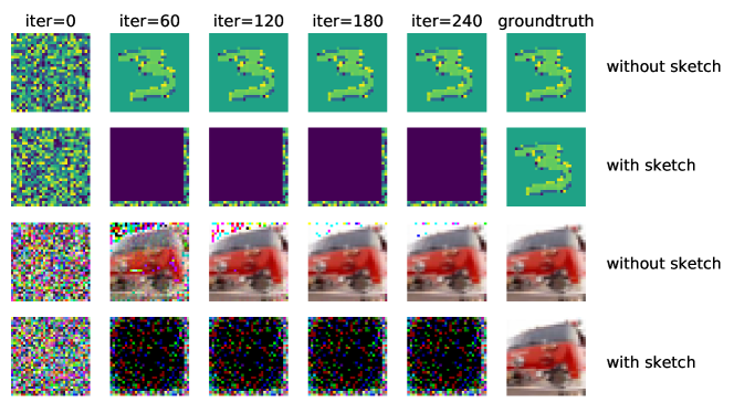
Figure 4: The images are generated by the gradient-matching attack of (Zhu et al., 2019). The attack is effective for the standard CNNs. Using sketching, the gradient-matching attack cannot recover the images.

Appendix B Algorithm Derivation

In this section, we derive the algorithm outlined in Section 4. In Section B.1 and B.2, we apply sketching to dense layer and convolutional layer, respectively, and derive the gradients.

B.1 Dense Layers

For simplicity, we study the case of batch size $b=1$ for a dense layer. Let ${\bf x}\in{\mathbb{R}}^{1\times{d_{\textrm{in}}}}$ be the input, ${\bf W}\in{\mathbb{R}}^{{d_{\textrm{out}}}\times{d_{\textrm{in}}}}$ be the parameter matrix, ${\bf S}\in{\mathbb{R}}^{{d_{\textrm{in}}}\times s}$ ($s<{d_{\textrm{in}}}$) be a sketching matrix, and

$${\bf z}\>=\>{\bf x}{\bf S}({\bf W}{\bf S})^{T}\in{\mathbb{R}}^{1\times{d_{\textrm{out}}}}$$

be the output (during training). For out-of-sample prediction, sketching is not applied, equivalently, ${\bf S}={\bf I}_{{d_{\textrm{in}}}}$.

In the following, we describe how to propagate gradient from the loss function back to ${\bf x}$ and ${\bf W}$. The dependence among the variables can be depicted as

$$\begin{array}[]{c}\textsf{input}\>\longrightarrow\>\cdots\>\longrightarrow\\ {}\hfil\end{array}\underbrace{\left.\begin{array}[]{c}{\bf x}\\ {\bf W}\\ \end{array}\right\}\>\longrightarrow\>{\bf z}}_{\textsf{the studied layer}}\>\longrightarrow\>\cdots\>\longrightarrow\>\textsf{loss}.$$

During the backpropagation, the gradients propagated to the studied layer are

$${\bf g}\>\triangleq\>\frac{\partial\,L}{\partial\,{\bf z}}\>\in\>{\mathbb{R}}^{1\times{d_{\textrm{out}}}},$$ (6)

where $L$ is some loss function. Then we further propagate the gradient from ${\bf z}$ to ${\bf x}$ and ${\bf W}$:

$$\frac{\partial\,L}{\partial\,{\bf x}}\>=\>\frac{\partial\,L}{\partial\,{\bf z}}\,\frac{\partial\,{\bf z}}{\partial\,({\bf x}{\bf S})}\,\frac{\partial\,({\bf x}{\bf S})}{\partial\,{\bf x}}\>=\>{\bf g}({\bf W}{\bf S}){\bf S}^{T}\>\in\>{\mathbb{R}}^{1\times{d_{\textrm{in}}}},$$ (7)

$$\frac{\partial\,L}{\partial\,{\bf W}}\>=\>{\bf g}^{T}({\bf x}{\bf S}){\bf S}^{T}\>\in\>{\mathbb{R}}^{{d_{\textrm{out}}}\times{d_{\textrm{in}}}}.$$ (8)

We prove (8) in the following. Let $\tilde{{\bf x}}={\bf x}{\bf S}\in{\mathbb{R}}^{1\times s}$ and $\widetilde{{\bf W}}={\bf W}{\bf S}\in{\mathbb{R}}^{{d_{\textrm{out}}}\times s}$. Let ${\bf w}_{j:}$ and $\tilde{{\bf w}}_{j:}$ be the $j$-th row of ${\bf W}$ and $\widetilde{{\bf W}}$, respectively. It can be shown that

$$\frac{\partial\,L}{\partial\,\tilde{{\bf w}}_{j:}}\>=\>\sum_{l=1}^{{d_{\textrm{out}}}}\frac{\partial\,L}{\partial\,z_{l}}\,\frac{\partial\,z_{l}}{\partial\,\tilde{{\bf w}}_{j:}}\>=\>\sum_{l=1}^{{d_{\textrm{out}}}}\frac{\partial\,L}{\partial\,z_{l}}\,\frac{\partial\,(\tilde{{\bf x}}\tilde{{\bf w}}_{l:}^{T})}{\partial\,\tilde{{\bf w}}_{j:}}\>=\>\frac{\partial\,L}{\partial\,z_{j}}\,\frac{\partial\,(\tilde{{\bf x}}\tilde{{\bf w}}_{j:}^{T})}{\partial\,\tilde{{\bf w}}_{j:}}\>=\>g_{j}\,\tilde{{\bf x}}\>\in\>{\mathbb{R}}^{1\times s}.$$

Thus, $\tilde{{\bf w}}_{j:}={\bf w}_{j:}{\bf S}\in{\mathbb{R}}^{1\times s}$; moreover, $\tilde{{\bf w}}_{j:}$ is independent of ${\bf w}_{l:}$ if $j\neq l$. It follows that

$$\frac{\partial\,L}{\partial\,{{\bf w}}_{j:}}\>=\>\frac{\partial\,L}{\partial\,\tilde{{\bf w}}_{j:}}\,\frac{\partial\,\tilde{{\bf w}}_{j:}}{\partial\,{{\bf w}}_{j:}}\>=\>g_{j}\,\tilde{{\bf x}}\,{\bf S}^{T}\>\in\>{\mathbb{R}}^{1\times{d_{\textrm{in}}}}.$$

Thus

$$\frac{\partial\,L}{\partial\,{\bf W}}\>=\>{\bf g}^{T}\,\tilde{{\bf x}}\,{\bf S}^{T}\>=\>{\bf g}^{T}({\bf x}{\bf S}){\bf S}^{T}\>\in\>{\mathbb{R}}^{{d_{\textrm{out}}}\times{d_{\textrm{in}}}}.$$

B.2 Extension to Convolutional Layers

Let ${\bf X}$ be a $d_{1}\times d_{2}\times d_{3}$ tensor and ${\bf K}$ be a $k_{1}\times k_{2}\times d_{3}$ kernel. The convolution ${\bf X}*{\bf K}$ outputs a $d_{1}\times d_{2}$ matrix (assume zero-padding is used). The convolution can be equivalently written as matrix-vector multiplication in the following way.

We segment ${\bf X}$ to many patches of shape $k_{1}\times k_{2}\times d_{3}$ and then reshape every patch to a ${d_{\textrm{in}}}\triangleq k_{1}k_{2}d_{3}$-dimensional vector. Let ${\bf p}_{i}$ be the $i$-th patch (vector). Tensor ${\bf X}$ has $q\triangleq d_{1}d_{2}$ such patches. Let

$${\bf P}\triangleq[{\bf p}_{1},\cdots,{\bf p}_{q}]^{T}\in{\mathbb{R}}^{q\times{d_{\textrm{in}}}}$$

be the concatenation of the patches. Let ${\bf w}\in{\mathbb{R}}^{{d_{\textrm{in}}}}$ be the vectorization of the kernel ${\bf K}\in{\mathbb{R}}^{k_{1}\times k_{2}\times d_{3}}$. The matrix-vector product, ${\bf z}={\bf P}{\bf w}\in{\mathbb{R}}^{q}$, is indeed the vectorization of the convolution ${\bf X}*{\bf K}$.

In practice, we typically use multiple kernels for the convolution; let ${\bf W}\triangleq[{\bf w}_{1},\cdots,{\bf w}_{{d_{\textrm{out}}}}]^{T}\in{\mathbb{R}}^{{d_{\textrm{out}}}\times{d_{\textrm{in}}}}$ be the concatenation of ${d_{\textrm{out}}}$ different (vectorized) kernels. In this way, the convolution of ${\bf X}$ with ${d_{\textrm{out}}}$ different kernels, which outputs a $d_{1}\times d_{2}\times r$ tensor, is the reshape of ${\bf X}{\bf W}^{T}\in{\mathbb{R}}^{q\times{d_{\textrm{out}}}}$.

We show in the above that tensor convolution can be equivalently expressed as matrix-matrix multiplication. Therefore, we can apply matrix sketching to convolutional layers in the same way as the dense layer. Specifically, let ${\bf S}$ be a ${d_{\textrm{in}}}\times s$ random sketching matrix. Then ${\bf X}{\bf S}({\bf W}{\bf S})^{T}$ is an approximation to ${\bf X}{\bf W}^{T}$, and the backpropagation is accordingly derived using matrix differentiation.

Appendix C Proofs

In this section, we prove Theorem 2 and Corollary 3. Theorem 2 follows from Lemmas 4 and 5. Corollary 3 follows from Lemma 6. Theorem 1 is a trivial consequence of Theorem 2.

Lemma 4.

Let ${\bf S}_{\textrm{old}}$ and ${\bf S}_{\textrm{new}}$ be independent CountSketch matrices. For any matrix ${\bf V}$ independent of ${\bf S}_{\textrm{old}}$ and ${\bf S}_{\textrm{new}}$, the following identity holds:

$${\mathbb{E}}\big{\|}\widehat{{\boldsymbol{\Delta}}}{\bf V}^{T}-{\boldsymbol{\Delta}}{\bf V}^{T}\big{\|}_{F}^{2}$$

$$=\>{\mathbb{E}}\big{\|}{\bf W}_{\textrm{old}}{\bf V}^{T}-{\bf W}_{\textrm{old}}{\bf S}_{\textrm{old}}{\bf S}_{\textrm{old}}^{T}{\bf V}^{T}\big{\|}_{F}^{2}+{\mathbb{E}}\big{\|}{\bf W}_{\textrm{new}}{\bf V}^{T}-{\bf W}_{\textrm{new}}{\bf S}_{\textrm{new}}{\bf S}_{\textrm{new}}^{T}{\bf V}^{T}\big{\|}_{F}^{2},$$

where the expectation is taken w.r.t. the random sketching matrices ${\bf S}_{\textrm{old}}$ and ${\bf S}_{\textrm{new}}$.

Proof.

Recall the definitions: ${\boldsymbol{\Delta}}={\bf W}_{\textrm{old}}-{\bf W}_{\textrm{new}}$ and $\widehat{{\boldsymbol{\Delta}}}={\bf W}_{\textrm{old}}{\bf S}_{\textrm{old}}{\bf S}_{\textrm{old}}^{T}-{\bf W}_{\textrm{new}}{\bf S}_{\textrm{new}}{\bf S}_{\textrm{new}}^{T}$. Then

$$\big{\|}\widehat{{\boldsymbol{\Delta}}}{\bf V}^{T}-{\boldsymbol{\Delta}}{\bf V}^{T}\big{\|}_{F}^{2}\>=\>\Big{\|}\big{(}{\bf W}_{\textrm{old}}{\bf S}_{\textrm{old}}{\bf S}_{\textrm{old}}^{T}-{\bf W}_{\textrm{new}}{\bf S}_{\textrm{new}}{\bf S}_{\textrm{new}}^{T}\big{)}{\bf V}^{T}-{\boldsymbol{\Delta}}{\bf V}^{T}\Big{\|}_{F}^{2}$$

$$=\>\Big{\|}\big{(}{\bf W}_{\textrm{old}}{\bf S}_{\textrm{old}}{\bf S}_{\textrm{old}}^{T}-{\bf W}_{\textrm{new}}{\bf S}_{\textrm{new}}{\bf S}_{\textrm{new}}^{T}\big{)}{\bf V}^{T}-({\bf W}_{\textrm{old}}-{\bf W}_{\textrm{new}}){\bf V}^{T}\Big{\|}_{F}^{2}$$

$$=\>\Big{\|}{\bf W}_{\textrm{old}}\big{(}{\bf S}_{\textrm{old}}{\bf S}_{\textrm{old}}^{T}-{\bf I}\big{)}{\bf V}^{T}+{\bf W}_{\textrm{new}}\big{(}{\bf I}-{\bf S}_{\textrm{new}}{\bf S}_{\textrm{new}}^{T}\big{)}{\bf V}^{T}\Big{\|}_{F}^{2}$$

$$=\>\big{\|}{\bf W}_{\textrm{old}}\big{(}{\bf S}_{\textrm{old}}{\bf S}_{\textrm{old}}^{T}-{\bf I}\big{)}{\bf V}^{T}\big{\|}_{F}^{2}+\big{\|}{\bf W}_{\textrm{new}}\big{(}{\bf I}-{\bf S}_{\textrm{new}}{\bf S}_{\textrm{new}}^{T}\big{)}{\bf V}^{T}\big{\|}_{F}^{2}$$

$$\quad+2\Big{\langle}{\bf W}_{\textrm{old}}\big{(}{\bf S}_{\textrm{old}}{\bf S}_{\textrm{old}}^{T}-{\bf I}\big{)}{\bf V}^{T},\;{\bf W}_{\textrm{new}}\big{(}{\bf I}-{\bf S}_{\textrm{new}}{\bf S}_{\textrm{new}}^{T}\big{)}{\bf V}^{T}\Big{\rangle}.$$

Since ${\mathbb{E}}[{\bf S}_{\textrm{old}}{\bf S}_{\textrm{old}}^{T}-{\bf I}]={\bf 0}$, ${\mathbb{E}}[{\bf S}_{\textrm{new}}{\bf S}_{\textrm{new}}^{T}-{\bf I}]={\bf 0}$, and ${\bf S}_{\textrm{old}}$ and ${\bf S}_{\textrm{new}}$ are independent, we have

$${\mathbb{E}}\Big{[}\Big{\langle}{\bf W}_{\textrm{old}}\big{(}{\bf S}_{\textrm{old}}{\bf S}_{\textrm{old}}^{T}-{\bf I}\big{)}{\bf V}^{T},\;{\bf W}_{\textrm{new}}\big{(}{\bf I}-{\bf S}_{\textrm{new}}{\bf S}_{\textrm{new}}^{T}\big{)}{\bf V}^{T}\Big{\rangle}\Big{]}\>=\>0.$$

It follows that

$${\mathbb{E}}\big{\|}\widehat{{\boldsymbol{\Delta}}}{\bf V}^{T}-{\boldsymbol{\Delta}}{\bf V}^{T}\big{\|}_{F}^{2}$$

$$=\>{\mathbb{E}}\big{\|}{\bf W}_{\textrm{old}}\big{(}{\bf S}_{\textrm{old}}{\bf S}_{\textrm{old}}^{T}-{\bf I}\big{)}{\bf V}^{T}\big{\|}_{F}^{2}+{\mathbb{E}}\big{\|}{\bf W}_{\textrm{new}}\big{(}{\bf I}-{\bf S}_{\textrm{new}}{\bf S}_{\textrm{new}}^{T}\big{)}{\bf V}^{T}\big{\|}_{F}^{2},$$

by which the lemma follows. ∎

Lemma 5.

Let ${\bf S}$ be a ${d\times s}$ CountSketch matrix. Let ${\bf A}\in{\mathbb{R}}^{n\times d}$ and ${\bf B}\in{\mathbb{R}}^{m\times d}$ be any non-random matrices. Then

$${\mathbb{E}}\big{[}{\bf A}{\bf S}{\bf S}^{T}{\bf B}^{T}-{\bf A}{\bf B}^{T}\big{]}^{2}\>=\>\frac{1}{s}\sum_{i=1}^{n}\sum_{j=1}^{m}\bigg{(}\sum_{k\neq l}a_{ki}^{2}b_{lj}^{2}+\sum_{k\neq l}a_{ki}b_{kj}a_{li}b_{lj}\bigg{)}.$$

Proof.

(Pham & Pagh, 2013; Weinberger et al., 2009) showed that for any vectors ${\bf a},{\bf b}\in{\mathbb{R}}^{d}$,

$${\mathbb{E}}\big{[}{\bf a}^{T}{\bf S}{\bf S}^{T}{\bf b}\big{]}\>=\>{\bf a}^{T}{\bf b},$$

$${\mathbb{E}}\big{[}{\bf a}^{T}{\bf S}{\bf S}^{T}{\bf b}-{\bf a}^{T}{\bf b}\big{]}^{2}\>=\>\frac{1}{s}\Big{(}\sum_{k\neq l}a_{k}^{2}b_{l}^{2}+\sum_{k\neq l}a_{k}b_{k}a_{l}b_{l}\Big{)}.$$

Let ${\bf a}_{i:}\in{\mathbb{R}}^{d}$ be the $i$-th row of ${\bf A}\in{\mathbb{R}}^{n\times d}$ and ${\bf b}_{j:}\in{\mathbb{R}}^{d}$ be the $j$-th column of ${\bf B}\in{\mathbb{R}}^{m\times d}$. Then,

$${\mathbb{E}}\big{[}{\bf A}{\bf S}{\bf S}^{T}{\bf B}^{T}-{\bf A}{\bf B}^{T}\big{]}^{2}\>=\>\sum_{i=1}^{n}\sum_{j=1}^{m}{\mathbb{E}}\big{[}{\bf a}_{i:}^{T}{\bf S}{\bf S}^{T}{\bf b}_{j:}-{\bf a}_{i:}^{T}{\bf b}_{j:}\big{]}^{2}$$

$$=\>\frac{1}{s}\sum_{i=1}^{n}\sum_{j=1}^{m}\bigg{(}\sum_{k\neq l}a_{ik}^{2}b_{jl}^{2}+\sum_{k\neq l}a_{ik}b_{jk}a_{il}b_{jl}\bigg{)},$$

by which the lemma follows. ∎

Lemma 6.

Let ${\bf S}$ be a ${d\times s}$ CountSketch matrix. Assume that the entries of ${\bf A}$ are IID and that the entries of ${\bf B}$ are also IID. Then

$${\mathbb{E}}\big{[}{\bf A}^{T}{\bf S}{\bf S}^{T}{\bf B}-{\bf A}^{T}{\bf B}\big{]}^{2}\>=\>\Theta\Big{(}\frac{d}{s}\Big{)}\|{\bf A}{\bf B}^{T}\|_{F}^{2}.$$

Proof.

Assume all the entries of ${\bf A}$ are IID sampled from a distribution with mean $\mu_{A}$ and standard deviation $\sigma_{A}$; assume all the entries of ${\bf B}$ are IID sampled from a distribution with mean $\mu_{B}$ and standard deviation $\sigma_{B}$. It follows from Lemma 5 that

$${\mathbb{E}}\big{[}{\bf A}{\bf S}{\bf S}^{T}{\bf B}^{T}-{\bf A}{\bf B}^{T}\big{]}^{2}\>=\>\frac{mn}{s}\big{[}(d^{2}-d)(\mu_{A}^{2}+\sigma_{A}^{2})(\mu_{B}^{2}+\sigma_{B}^{2})+(d^{2}-d)\mu_{A}^{2}\mu_{B}^{2}\big{]}$$

$$=\>\Theta\Big{(}\frac{mnd^{2}}{s}(\mu_{A}^{2}+\sigma_{A}^{2})(\mu_{B}^{2}+\sigma_{B}^{2})\Big{)}\>=\>\Theta\Big{(}\frac{d}{s}\Big{)}\|{\bf A}{\bf B}^{T}\|_{F}^{2}.$$

∎

Appendix D Decentralized Learning

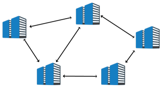
Figure 5: Decentralized learning in a peer-to-peer network.

Instead of relying on a central server, multiple parties can collaborate using such a peer-to-peer network as Figure 5. A client is a compute node in the graph and connected to a few neighboring nodes. Many decentralized optimization algorithms have been developed (Bianchi et al., 2013; Yuan et al., 2016; Sirb & Ye, 2016; Colin et al., 2016; Lian et al., 2017; Lan et al., 2017; Tang et al., 2018). The nodes collaborate by, for example, aggregating its neighbors’ model parameters, taking a weighted average of neighbors’ and its own parameters as the intermediate parameters, and then locally performing an SGD update.

We find that the attacks of (Melis et al., 2019; Zhu et al., 2019) can be applied to this kind of decentralized learning. Note that a node shares its model parameters with its neighbors. If a node is malicious, it can use its neighbors’ gradients and model parameters to infer their data. Let a neighbor’s (the victim) parameters in two consecutive rounds be ${\bf W}_{\textrm{old}}$ and ${\bf W}_{\textrm{new}}$. The difference, ${\boldsymbol{\Delta}}={\bf W}_{\textrm{old}}-{\bf W}_{\textrm{new}}$, is mainly the gradient evaluated on the victim’s data. With the model parameters ${\bf W}$ and updating direction ${\boldsymbol{\Delta}}$ at hand, the attacker can perform the gradient-based attacks of (Melis et al., 2019; Zhu et al., 2019).

Our DBCL can be easily applied under the decentralized setting: two neighboring compute nodes agree upon the random seeds, sketching their model parameters, and communicate the sketches. This can stop any node from knowing, ${\boldsymbol{\Delta}}={\bf W}_{\textrm{old}}-{\bf W}_{\textrm{new}}$, i.e., the gradient of the neighbor. We will empirically study the decentralized setting in our future work.

Appendix E Code of Core Algorithms

The following code implements the CountSketch and transposed CountSketch. Given matrix ${\bf A}$, the CountSketch outputs ${\bf C}={\bf A}{\bf S}$. Given ${\bf C}$, the transposed CountSketch outputs ${\bf B}={\bf C}{\bf S}^{T}$.

⬇

1class Sketch():

2

3 # Random Hashing

4 # Generate random indices and random signs

5 # Args:

6 # n: (integer) number of items to be hashed

7 # q: (integer) map n items to a table of s=n/q rows

8 # Return:

9 # hash_idx: (q-by-s Torch Tensor) contain random integer in {0, 1, …, s-1}

10 # rand_sgn: (n-by-1 Torch Tensor) contain random signs (+1 or -1)

11 def rand_hashing(n, q):

12 s = math.floor(n / q)

13 t = torch.randperm(n)

14 hash_idx = t[0:(s * q)].reshape((q, s))

15 rand_sgn = torch.randint(0, 2, (n,)).float() * 2 - 1

16 return hash_idx, rand_sgn

17

18 # Count sketch

19 # It converts m-by-n matrix to m-by-s matrix

20 # Args:

21 # a: (m-by-n Torch Tensor) input matrix

22 # hash_idx: (q-by-s Torch Tensor) contain random integer in {0, 1, …, s-1}

23 # rand_sgn: (n-by-1 Torch Tensor) contain random signs (+1 or -1)

24 # Return:

25 # c: m-by-s sketch (Torch Tensor) (result of count sketch)

26 def countsketch(a, hash_idx, rand_sgn):

27 m, n = a.shape

28 s = hash_idx.shape[1]

29 c = torch.zeros([m, s], dtype=torch.float32)

30 b = a.mul(rand_sgn)

31

32 for h in range(s):

33 selected = hash_idx[:, h]

34 c[:, h] = torch.sum(b[:, selected], dim=1)

35

36 return c

37

38 # Transpose count sketch

39 # The ”countsketch” function converts m-by-n matrix A to m-by-s matrix C

40 # This function maps C back to a m-by-n matrix B

41 # Args:

42 # c: (m-by-s Torch Tensor) input matrix

43 # hash_idx: (q-by-s Torch Tensor) contain random integer in {0, 1, …, s-1}

44 # rand_sgn: (n-by-1 Torch Tensor) contain random signs (+1 or -1)

45 # Return:

46 # b: m-by-n matrix

47 def transpose_countsketch(c, hash_idx, rand_sgn):

48 m, s = c.shape

49 n = len(rand_sgn)

50 b = torch.zeros([m, n], dtype=torch.float32)

51 for h in range(s):

52 selected = hash_idx[:, h]

53 b[:, selected] = c[:, h].reshape(m, 1)

54 b = b.mul(rand_sgn)

55 return b

The standard linear function of PyTorch computes ${\bf Z}={\bf X}{\bf W}^{T}+{\bf B}$, where ${\bf X}$ is a batch of inputs, ${\bf W}$ is the weight matrix, and ${\bf B}$ is the bias (aka intercept). With CountSketch applied, the output becomes ${\bf Z}={\bf X}{\bf S}{\bf S}^{T}{\bf W}^{T}+{\bf B}$. We need to implement both the forward function and the backward function. The backward function is called during backpropagation.

⬇

1class SketchLinearFunction(torch.autograd.Function):

2 @staticmethod

3 def forward(ctx, input, weight, bias, hash_idx, rand_sgn, training=True, q=2):

4 if training:

5 # input_features = weight.shape[-1]

6

7 # sketching the input and weight matrices

8 # hash_idx, rand_sgn = Sketch.rand_hashing(input_features, q)

9 input_sketch = Sketch.countsketch(input, hash_idx, rand_sgn)

10 weight_sketch = Sketch.countsketch(weight, hash_idx, rand_sgn)

11 output = input_sketch.mm(weight_sketch.t())

12

13 ctx.save_for_backward(input_sketch, weight_sketch, bias, hash_idx, rand_sgn)

14 else:

15 output = input.mm(weight.t())

16

17 output += bias.unsqueeze(0).expand_as(output)

18 return output

19

20 @staticmethod

21 def backward(ctx, grad_output):

22 input_sketch, weight_sketch, bias, hash_idx, rand_sgn = ctx.saved_tensors

23 grad_input = grad_weight = grad_bias = grad_training = None

24

25 if ctx.needs_input_grad[0]:

26 grad_input_tmp = grad_output.mm(weight_sketch)

27 grad_input = Sketch.transpose_countsketch(grad_input_tmp, hash_idx, rand_sgn)

28 if ctx.needs_input_grad[1]:

29 grad_weight_tmp = grad_output.t().mm(input_sketch)

30 grad_weight = Sketch.transpose_countsketch(grad_weight_tmp, hash_idx, rand_sgn)

31 if ctx.needs_input_grad[2]:

32 grad_bias = grad_output.sum(0).squeeze(0)

33

34 return grad_input, grad_weight, grad_bias, None, None, None, None

The following PyTorch code applies CountSketch to the parameter matrices of a dense layer (aka linear layer or fully-connected layer).

⬇

1class SketchLinear(nn.Module):

2 def __init__(self, input_features, output_features, q=2):

3 super(SketchLinear, self).__init__()

4 self.input_features = input_features

5 self.output_features = output_features

6 self.q = q

7

8 self.weight = nn.Parameter(torch.Tensor(output_features, input_features))

9 self.bias = nn.Parameter(torch.Tensor(output_features))

10 self.register_parameter(’weight’, self.weight)

11 self.register_parameter(’bias’, self.bias)

12

13 bound = 1 / math.sqrt(input_features)

14 scaling = math.sqrt(3.0)

15 self.weight.data.uniform_(-bound * scaling, bound * scaling)

16 self.bias.data.uniform_(-bound, bound)

17

18 def forward(self, input, hash_idx, rand_sgn):

19 return SketchLinearFunction.apply(input, self.weight, self.bias, hash_idx, rand_sgn, self.training, self.q)

20

21 def extra_repr(self):

22 return ’input_features={}, output_features={}, weight={}, bias={}’.format(

23 self.input_features, self.output_features, self.weight, self.bias

24 )

The following code applies CountSketch to the convolution function of PyTorch. We express convolution as matrix multiplication, and then apply CountSketch in the same way as above.

⬇

1class SketchConvFunction(torch.autograd.Function):

2 @staticmethod

3 def forward(ctx, input, weight, bias, k, hash_idx, rand_sgn, training=True, q=2):

4 ”’

5 Args:

6 input: shape=(b, c0, w0, h0)

7 weight: shape=(c1, c0*k*k)

8 bias: shape=(c1)

9 k: number of kernels

10

11 Return:

12 output: shape=(b, c1, w1, h1)

13

14 Note:

15 b: batch size

16 c0: number of input channels

17 c1: number of output channels

18 ’”

19 b, c0, w0, h0 = input.shape

20 c1 = weight.shape[0]

21 w1 = w0 + 1 - k

22 h1 = h0 + 1 - k

23

24 # input tensor (b, c0, w0, h0) to patches (b*w1*h1, k*k*c0)

25 fan_in = k * k * c0

26 x = nn.functional.unfold(input, (k, k)).transpose(1, 2).reshape(b * w1 * h1, fan_in)

27

28 if training:

29 # sketching the input and weight matrices

30 # hash_idx, rand_sgn = Sketch.rand_hashing(fan_in, q)

31 x_sketch = Sketch.countsketch(x, hash_idx, rand_sgn)

32 weight_sketch = Sketch.countsketch(weight, hash_idx, rand_sgn)

33 z = x_sketch.matmul(weight_sketch.t()) # shape=(b*w1*h1, c1)

34

35 # save for backprop

36 shapes = torch.IntTensor([k, b, c0, w0, h0, c1, w1, h1])

37 ctx.save_for_backward(x_sketch, weight_sketch, bias, shapes, hash_idx, rand_sgn)

38 else:

39 # the multiplication of x and w transpose

40 z = x.matmul(weight.t()) # shape=(b*w1*h1, c1)

41

42 # add bias

43 bias_expand = bias.reshape(1, c1).expand([b * w1 * h1, c1])

44 out_reshape = z + bias_expand # shape=(b*w1*h1, c1)

45 output = out_reshape.reshape(b, w1 * h1, c1).transpose(1, 2).reshape(b, c1, w1, h1)

46

47 return output

48

49 @staticmethod

50 def backward(ctx, grad_output):

51 x_sketch, weight_sketch, bias, shapes, hash_idx, rand_sgn = ctx.saved_tensors

52 grad_input = grad_weight = grad_bias = None

53 k, b, c0, w0, h0, c1, w1, h1 = shapes

54

55 grad_output1 = grad_output.view(b, c1, -1).transpose(1, 2).reshape(b * w1 * h1, c1) # shape=(b*w1*h1, c1)

56

57 if ctx.needs_input_grad[0]:

58 grad_x0 = grad_output1.matmul(weight_sketch) # shape=(b*w1*h1, s)

59 grad_x1 = Sketch.transpose_countsketch(grad_x0, hash_idx, rand_sgn) # shape=(b*w1*h1, c0*k*k)

60 grad_x2 = grad_x1.reshape(b, w1 * h1, c0 * k * k).transpose(1, 2)

61 grad_input = nn.functional.fold(grad_x2, (w0, h0), (k, k)) # shape=(b, c0, w0, h0)

62 if ctx.needs_input_grad[1]:

63 grad_w_sketch = grad_output1.t().matmul(x_sketch) # shape=(c1, s)

64 grad_weight = Sketch.transpose_countsketch(grad_w_sketch, hash_idx, rand_sgn) # shape=(c1, c0*k*k)

65 if ctx.needs_input_grad[2]:

66 grad_bias = grad_output1.sum(0)

67

68 return grad_input, grad_weight, grad_bias, None, None, None, None, None

The following PyTorch code applies CountSketch to the parameter matrices of a convolutional layer.

⬇

1class SketchConv(nn.Module):

2 def __init__(self, in_channels, out_channels, kernel_size, q=2):

3 super(SketchConv, self).__init__()

4 self.in_channels = in_channels

5 self.out_channels = out_channels

6 self.kernel_size = kernel_size

7 self.q = q

8

9 self.weight = nn.Parameter(torch.Tensor(out_channels, in_channels * kernel_size * kernel_size))

10 self.bias = nn.Parameter(torch.Tensor(out_channels))

11 self.register_parameter(’weight’, self.weight)

12 self.register_parameter(’bias’, self.bias)

13

14 # uniform initialization

15 scaling = math.sqrt(6.0)

16 bound = 1 / math.sqrt(in_channels * kernel_size * kernel_size)

17 self.weight.data.uniform_(-bound * scaling, bound * scaling)

18 self.bias.data.uniform_(-bound, bound)

19

20 def forward(self, input, hash_idx, rand_sgn):

21 return SketchConvFunction.apply(input, self.weight, self.bias, self.kernel_size, hash_idx, rand_sgn, self.training, self.q)

22

23 def extra_repr(self):

24 return ’in_channels={}, out_channels={}, kernel_size={}, weight={}, bias={}’.format(

25 self.in_channels, self.out_channels, self.kernel_size, self.weight, self.bias

26 )

References

- Aono et al. (2017) Aono, Y., Hayashi, T., Wang, L., Moriai, S., et al. Privacy-preserving deep learning via additively homomorphic encryption. IEEE Transactions on Information Forensics and Security, 13(5):1333–1345, 2017.
- Ateniese et al. (2015) Ateniese, G., Mancini, L. V., Spognardi, A., Villani, A., Vitali, D., and Felici, G. Hacking smart machines with smarter ones: How to extract meaningful data from machine learning classifiers. International Journal of Security and Networks, 10(3):137–150, September 2015. ISSN 1747-8405.
- Bianchi et al. (2013) Bianchi, P., Fort, G., and Hachem, W. Performance of a distributed stochastic approximation algorithm. IEEE Transactions on Information Theory, 59(11):7405–7418, 2013.
- Blocki et al. (2012) Blocki, J., Blum, A., Datta, A., and Sheffet, O. The Johnson-Lindenstrauss transform itself preserves differential privacy. In Annual Symposium on Foundations of Computer Science (FOCS), 2012.
- Bonawitz et al. (2017) Bonawitz, K., Ivanov, V., Kreuter, B., Marcedone, A., McMahan, H. B., Patel, S., Ramage, D., Segal, A., and Seth, K. Practical secure aggregation for privacy preserving machine learning. IACR Cryptology ePrint Archive, 2017:281, 2017.
- Charikar et al. (2004) Charikar, M., Chen, K., and Farach-Colton, M. Finding frequent items in data streams. Theoretical Computer Science, 312(1):3–15, 2004.
- Chen et al. (2018) Chen, Q., Xiang, C., Xue, M., Li, B., Borisov, N., Kaarfar, D., and Zhu, H. Differentially private data generative models. arXiv preprint arXiv:1812.02274, 2018.
- Clarkson & Woodruff (2013) Clarkson, K. L. and Woodruff, D. P. Low rank approximation and regression in input sparsity time. In Annual ACM Symposium on theory of computing (STOC), 2013.
- Colin et al. (2016) Colin, I., Bellet, A., Salmon, J., and Clémenccon, S. Gossip dual averaging for decentralized optimization of pairwise functions. arXiv preprint arXiv:1606.02421, 2016.
- Drineas & Mahoney (2016) Drineas, P. and Mahoney, M. W. RandNLA: randomized numerical linear algebra. Communications of the ACM, 59(6):80–90, 2016.
- Drineas et al. (2008) Drineas, P., Mahoney, M. W., and Muthukrishnan, S. Relative-error CUR matrix decompositions. SIAM Journal on Matrix Analysis and Applications, 30(2):844–881, September 2008.
- Dwork (2011) Dwork, C. Differential privacy. Encyclopedia of Cryptography and Security, pp. 338–340, 2011.
- Dwork & Naor (2010) Dwork, C. and Naor, M. On the difficulties of disclosure prevention in statistical databases or the case for differential privacy. Journal of Privacy and Confidentiality, 2(1), 2010.
- Fredrikson et al. (2015) Fredrikson, M., Jha, S., and Ristenpart, T. Model inversion attacks that exploit confidence information and basic countermeasures. In Proceedings of the 22nd ACM SIGSAC Conference on Computer and Communications Security, 2015.
- Giacomelli et al. (2018) Giacomelli, I., Jha, S., Joye, M., Page, C. D., and Yoon, K. Privacy-preserving ridge regression with only linearly-homomorphic encryption. In International Conference on Applied Cryptography and Network Security, pp. 243–261. Springer, 2018.
- Gilad-Bachrach et al. (2016) Gilad-Bachrach, R., Dowlin, N., Laine, K., Lauter, K., Naehrig, M., and Wernsing, J. CryptoNets: Applying neural networks to encrypted data with high throughput and accuracy. In International Conference on Machine Learning (ICML), 2016.
- Halko et al. (2011) Halko, N., Martinsson, P.-G., and Tropp, J. A. Finding structure with randomness: Probabilistic algorithms for constructing approximate matrix decompositions. SIAM Review, 53(2):217–288, 2011.
- Hanzely et al. (2018) Hanzely, F., Mishchenko, K., and Richtárik, P. SEGA: Variance reduction via gradient sketching. In Advances in Neural Information Processing Systems (NeurIPS), 2018.
- Hitaj et al. (2017) Hitaj, B., Ateniese, G., and Perez-Cruz, F. Deep models under the GAN: information leakage from collaborative deep learning. In Proceedings of the 2017 ACM SIGSAC Conference on Computer and Communications Security, 2017.
- Johnson & Lindenstrauss (1984) Johnson, W. B. and Lindenstrauss, J. Extensions of Lipschitz mappings into a Hilbert space. Contemporary mathematics, 26(189-206), 1984.
- Kenthapadi et al. (2012) Kenthapadi, K., Korolova, A., Mironov, I., and Mishra, N. Privacy via the Johnson-Lindenstrauss transform. arXiv preprint arXiv:1204.2606, 2012.
- Khaled & Richtárik (2019) Khaled, A. and Richtárik, P. Gradient descent with compressed iterates. arXiv, 2019.
- Koloskova et al. (2019) Koloskova, A., Stich, S. U., and Jaggi, M. Decentralized stochastic optimization and gossip algorithms with compressed communication. arXiv preprint arXiv:1902.00340, 2019.
- Lan et al. (2017) Lan, G., Lee, S., and Zhou, Y. Communication-efficient algorithms for decentralized and stochastic optimization. Mathematical Programming, pp. 1–48, 2017.
- Li et al. (2019a) Li, T., Liu, Z., Sekar, V., and Smith, V. Privacy for free: Communication-efficient learning with differential privacy using sketches. arXiv preprint arXiv:1911.00972, 2019a.
- Li et al. (2019b) Li, X., Huang, K., Yang, W., Wang, S., and Zhang, Z. On the convergence of FedAvg on Non-IID data. arXiv:1907.02189, 2019b.
- Lian et al. (2017) Lian, X., Zhang, C., Zhang, H., Hsieh, C.-J., Zhang, W., and Liu, J. Can decentralized algorithms outperform centralized algorithms? a case study for decentralized parallel stochastic gradient descent. In Advances in Neural Information Processing Systems (NIPS), 2017.
- Liu et al. (2018) Liu, Y., Chen, T., and Yang, Q. Secure federated transfer learning. arXiv preprint arXiv:1812.03337, 2018.
- Luo et al. (2019) Luo, Q., He, J., Zhuo, Y., and Qian, X. Heterogeneity-aware asynchronous decentralized training. arXiv preprint arXiv:1909.08029, 2019.
- Mahoney (2011) Mahoney, M. W. Randomized algorithms for matrices and data. Foundations and Trends in Machine Learning, 3(2):123–224, 2011.
- Martinsson & Tropp (2020) Martinsson, P.-G. and Tropp, J. Randomized numerical linear algebra: Foundations & algorithms. arXiv preprint arXiv:2002.01387, 2020.
- McMahan et al. (2017) McMahan, B., Moore, E., Ramage, D., Hampson, S., and y Arcas, B. A. Communication-efficient learning of deep networks from decentralized data. In Artificial Intelligence and Statistics (AISTATS), 2017.
- Melis et al. (2019) Melis, L., Song, C., De Cristofaro, E., and Shmatikov, V. Exploiting unintended feature leakage in collaborative learning. In IEEE Symposium on Security and Privacy (SP), 2019.
- Meng & Mahoney (2013) Meng, X. and Mahoney, M. W. Low-Distortion Subspace Embeddings in Input-Sparsity Time and Applications to Robust Linear Regression. In Annual ACM Symposium on Theory of Computing (STOC), 2013.
- Nelson & Nguyên (2013) Nelson, J. and Nguyên, H. L. OSNAP: Faster Numerical Linear Algebra Algorithms via Sparser Subspace Embeddings. In IEEE Annual Symposium on Foundations of Computer Science (FOCS), 2013.
- Pham & Pagh (2013) Pham, N. and Pagh, R. Fast and scalable polynomial kernels via explicit feature maps. In ACM SIGKDD International Conference on Knowledge Discovery and Data Mining (KDD), 2013.
- Ram et al. (2010) Ram, S. S., Nedić, A., and Veeravalli, V. V. Asynchronous gossip algorithm for stochastic optimization: Constant stepsize analysis. In Recent Advances in Optimization and its Applications in Engineering, pp. 51–60. Springer, 2010.
- Rouhani et al. (2018) Rouhani, B. D., Riazi, M. S., and Koushanfar, F. DeepSecure: Scalable provably-secure deep learning. In Proceedings of the 55th Annual Design Automation Conference, 2018.
- Sahu et al. (2019) Sahu, A. K., Li, T., Sanjabi, M., Zaheer, M., Talwalkar, A., and Smith, V. Federated optimization for heterogeneous networks. arXiv preprint arXiv:1812.06127, 2019.
- Sirb & Ye (2016) Sirb, B. and Ye, X. Consensus optimization with delayed and stochastic gradients on decentralized networks. In 2016 IEEE International Conference on Big Data (Big Data), pp. 76–85. IEEE, 2016.
- Srivastava & Nedic (2011) Srivastava, K. and Nedic, A. Distributed asynchronous constrained stochastic optimization. IEEE Journal of Selected Topics in Signal Processing, 5(4):772–790, 2011.
- Srivastava et al. (2014) Srivastava, N., Hinton, G., Krizhevsky, A., Sutskever, I., and Salakhutdinov, R. Dropout: a simple way to prevent neural networks from overfitting. Journal of Machine Learning Research, 15(1):1929–1958, 2014.
- Stich (2018) Stich, S. U. Local SGD converges fast and communicates little. arXiv preprint arXiv:1805.09767, 2018.
- Tang et al. (2018) Tang, H., Lian, X., Yan, M., Zhang, C., and Liu, J. D2: Decentralized training over decentralized data. arXiv preprint arXiv:1803.07068, 2018.
- Thorup & Zhang (2012) Thorup, M. and Zhang, Y. Tabulation-based 5-independent hashing with applications to linear probing and second moment estimation. SIAM Journal on Computing, 41(2):293–331, April 2012. ISSN 0097-5397.
- Wager et al. (2013) Wager, S., Wang, S., and Liang, P. S. Dropout training as adaptive regularization. In Advances in Neural Information Processing Systems (NIPS), 2013.
- Wang & Joshi (2018) Wang, J. and Joshi, G. Cooperative SGD: A unified framework for the design and analysis of communication-efficient SGD algorithms. arXiv preprint arXiv:1808.07576, 2018.
- Wang et al. (2019) Wang, J., Sahu, A. K., Yang, Z., Joshi, G., and Kar, S. Matcha: Speeding up decentralized sgd via matching decomposition sampling. arXiv preprint arXiv:1905.09435, 2019.
- Weinberger et al. (2009) Weinberger, K., Dasgupta, A., Langford, J., Smola, A., and Attenberg, J. Feature hashing for large scale multitask learning. In International Conference on Machine Learning (ICML), 2009.
- Woodruff (2014) Woodruff, D. P. Sketching as a tool for numerical linear algebra. Foundations and Trends® in Theoretical Computer Science, 10(1–2):1–157, 2014.
- Yu et al. (2019) Yu, H., Yang, S., and Zhu, S. Parallel restarted sgd with faster convergence and less communication: Demystifying why model averaging works for deep learning. In AAAI Conference on Artificial Intelligence, 2019.
- Yuan & Yu (2013) Yuan, J. and Yu, S. Privacy preserving back-propagation neural network learning made practical with cloud computing. IEEE Transactions on Parallel and Distributed Systems, 25(1):212–221, 2013.
- Yuan et al. (2016) Yuan, K., Ling, Q., and Yin, W. On the convergence of decentralized gradient descent. SIAM Journal on Optimization, 26(3):1835–1854, 2016.
- Zhang et al. (2018a) Zhang, D., Chen, X., Wang, D., and Shi, J. A survey on collaborative deep learning and privacy-preserving. In IEEE Third International Conference on Data Science in Cyberspace (DSC), 2018a.
- Zhang et al. (2018b) Zhang, Q., Wang, C., Wu, H., Xin, C., and Phuong, T. V. GELU-Net: A globally encrypted, locally unencrypted deep neural network for privacy-preserved learning. In International Joint Conferences on Artificial Intelligence (IJCAI), 2018b.
- Zhou & Cong (2017) Zhou, F. and Cong, G. On the convergence properties of a k-step averaging stochastic gradient descent algorithm for nonconvex optimization. arXiv preprint arXiv:1708.01012, 2017.
- Zhu et al. (2019) Zhu, L., Liu, Z., and Han, S. Deep leakage from gradients. In Advances in Neural Information Processing Systems (NeurIPS), 2019.