Data-driven ambiguity sets with probabilistic guarantees for dynamic processes

Abstract

Distributional ambiguity sets provide quantifiable ways to characterize the uncertainty about the true probability distribution of random variables of interest. This makes them a key element in data-driven robust optimization by exploiting high-confidence guarantees to hedge against uncertainty. This paper explores the construction of Wasserstein ambiguity sets in dynamic scenarios where data is collected progressively and may only reveal partial information about the unknown random variable. For random variables evolving according to known dynamics, we leverage assimilated samples to make inferences about their unknown distribution at the end of the sampling horizon. Under exact knowledge of the flow map, we provide sufficient conditions that relate the growth of the trajectories with the sampling rate to establish a reduction of the ambiguity set size as the horizon increases. Further, we characterize the exploitable sample history that results in a guaranteed reduction of ambiguity sets under errors in the computation of the flow and when the dynamics is subject to bounded unknown disturbances. Our treatment deals with both full- and partial-state measurements and, in the latter case, exploits the sampled-data observability properties of linear time-varying systems under irregular sampling. Simulations on a UAV detection application show the superior performance resulting from the proposed dynamic ambiguity sets.

I Introduction

In stochastic optimization, ambiguity sets play a key role by accounting for ’what-if’ scenarios regarding the true probability distribution of random variables affecting the objective function or the constraints. Rigorous guarantees on the probability of these sets containing the true distribution allows the designer to robustify decisions in the face of uncertainty. This explains the numerous applications that distributionally robust optimization with ambiguity sets finds in decision making under uncertainty, reliability-based design, and data-driven modeling. Moving beyond the static problem, where full-state measurements on the random variable are available all at once, this paper instead looks at scenarios where the random variable evolves dynamically and data is collected incrementally. We are interested in developing methods to construct ambiguity sets and track their evolution across time while maintaining their probabilistic guarantees about the true distribution. These methods should handle exact and approximate knowledge of the dynamics, the presence of disturbances, and the availability of partial-state measurements of the random variable. We also seek to shed light on the trade-offs between data assimilation and accuracy of the resulting ambiguity sets.

Literature review: DRO optimization is an area of stochastic programming [27] which has gained significant recent research attention [13], [26], [7], in view of the progress on robust optimization during the last two decades [5]. A main characteristic of DRO is that worst-case decisions against model uncertainty can be quantified with performance guarantees, by considering a set of distributions up to a certain distance from a candidate model. There is an exhaustive number of choices for distances in spaces of probability distributions [24]. Among the most popular distance-type notions for DRO problems are $\phi$-divergences [6], [16], and Wasserstein metrics [15], [9]. For data-driven problems where robustness is measured with respect to the empirical distribution, the Wasserstein distance becomes a suitable choice, since it does not require any absolute continuity conditions between the associated distributions. The work [13] leverages recent concentration of measure inequalities [14] to build Wasserstein ambiguity sets around the empirical distribution of the data, and provides tractable reformulations of the associated DRO problems with out-of-sample guarantees. These are exploited in [11], where a distributed reformulation of the min-max DRO problem is established via saddle-point dynamics, and in [23], where online sample assimilation is fused with an efficient optimization algorithm to provide on-the-fly data-driven DRO solutions. It is worthwhile mentioning also the work [8], where the notion of a robust Wasserstein profile function is employed, providing fast asymptotic convergence rates for high-dimensional samples. Recent work has considered distributionally robust Kalman filtering approaches for the state estimation of uncertain time-varying processes for the Kullback-Leibler [22], $\tau$-divergences [34], and the Wasserstein [25] metrics.

Observability of linear and nonlinear systems occupies a central part of the control literature [28]. Of considerable practical interest is the case where the output of a system is not continuously measured and samples are collected instead. Classical results regarding observability for linear time-invariant systems under periodic sampling with equidistributed measurements can be found in [28]. For the same system class, a periodic sampling schedule which always maintains observability of the continuous plant was proposed in [20]. Observability under regular sampling for nonlinear models has been studied in [3] for systems on compact manifolds, in [1] for bilinear systems, and conditions under which the property become generic are given in [2]. Results on the asymptotic state estimation in the nonlinear case through sampled-data observes are derived in [17]. Also, the observability of linear time-invariant (LTI) systems under irregular sampling, using properties of exponential polynomials, has been studied in the recent works [31, 32], and exploited to establish observability of LTI ensembles in [33].

Statement of contributions: We consider dynamically evolving random variables of unknown distribution on which samples from multiple independent realizations are collected in an online fashion. Our contributions revolve around providing solutions to integrate the data to construct distributional ambiguity sets based on the Wasserstein metric that enjoy rigorous probabilistic guarantees. Throughout the technical approach, we pay attention to characterizing how the information contained in the incrementally collected data can be pushed forward in time to infer properties about the evolving distribution of the process. Under full-state measurements and exact pushforward through the flow, our first contribution builds ambiguity balls that incorporate past data to enjoy desirable guarantees on the probability of containing the true distribution. We also identify conditions on the growth of the dynamics of the random variable under which the ambiguity radius shrinks as the horizon increases. Our second contribution considers scenarios with approximate pushforwards and disturbances in the dynamics, and characterizes the modifications necessary in the ambiguity radius that retain the same high-confidence probabilistic guarantees. This result allows us to quantify the effective sampling horizon that ensures the monotonic reduction of the ambiguity set with the number of sampling times. To enable the extension of these results to the case with partial-state measurements, our third contribution studies robust sample-data observability under irregular sampling of linear time-varying systems. We provide conditions on the inter-sampling time of the trajectories under which full-state information can be extracted. Our final contribution is the construction of high-confidence distributional ambiguity sets under partial-state measurements. We illustrate our results in a UAV detection scenario application formulated as a distributionally robust optimization problem.

II Problem Formulation

A distributionally robust optimization problem (DROP) takes the form

$${\rm(P)}\qquad\qquad\inf_{x\in\mathcal{X}}\sup_{P\in\widehat{\mathcal{P}}^{N}}\mathbb{E}_{P}[f(x,\xi)],$$

where $x\in\mathcal{X}\subset\mathbb{R}^{n}$ is the decision variable and $\xi$ represents a random variable distributed according to a distribution $P_{\xi}\in{\mathcal{P}}({}^{d})$. This distribution is unknown and hence one formulates a worst-case expectation problem over an ambiguity set $\widehat{\mathcal{P}}^{N}$ which contains it with some probabilistic guarantee. Such guarantees can be obtained when data about the random variable is available: given $N$ i.i.d. samples $\xi^{1},\ldots,\xi^{N}$ drawn according to the unknown distribution $P_{\xi}$ and a reliability parameter $\beta\in(0,1)$, one can construct [13] an ambiguity set such that $\mathbb{P}(P_{\xi}\in\widehat{\mathcal{P}}^{N})\geq 1-\beta$. We refer to this common formulation as a static DROP. Here, we are interested in building the ambiguity set from dynamically varying, possibly partial data in an online manner, as it may not be feasible to collect and process many samples in a given time instant. We next present an illustrative example.

II-A Motivating example

Let $\xi_{t}=(\xi_{1t},\xi_{2t})$ describe the position and velocity of a unit acceleration particle, evolving according to the known dynamics

$$\dot{\xi}_{1t}=\xi_{2t},\quad\dot{\xi}_{2t}=1,$$

over a time horizon $[0,T]$. Assume that we can measure the position $\zeta_{t}=H(\xi_{t}):=\xi_{1t}$, but not the velocity. Then, taking two position measurements are sufficient to reconstruct the full state of the particle. Both its initial position and velocity are random with unknown probability distribution. Therefore, the particle state at each $t$ is a random variable with law $P_{\xi_{t}}$. Given that these distributions are unknown, we focus on specifying an ambiguity set $\widehat{\mathcal{P}}_{T}^{N}$ at time $T$ which contains the true distribution $P_{\xi_{T}}$ with high confidence. To do this, independent output samples from the distribution of $\zeta_{t}=H(\xi_{t})$ are available at time instants $0\leq t_{1}<\ldots<t_{\bar{N}}=T$, cf. Figure 1. In this scenario, a direct application of the conventional approach to static DROPs would only employ the samples obtained at $t_{\bar{N}}$ to construct the ambiguity set and solve (P). This would not be desirable because (i) constructing reliable ambiguity sets requires a finite, but sufficiently large amount of data, and (ii) the output map reveals information about the particle’s position, but not about its velocity.

Figure 1: Partial measurements across a sequence of time instants of trajectories of the random variable can be exploited to generate samples of the full-state distribution at $T$. The latter can be employed to construct ambiguity sets that contain the true unknown distribution with high confidence. The blue curves show how the probability density of the state distribution evolves over time. We display the output samples with the red stars and use a bent arrow to represent the output map applied to the trajectories’ states at the sampling instants. Each yellow star depicts either the reconstructed state of a trajectory once the last output sample is collected from it, or its corresponding value pushed forward to $t_{\bar{N}}=T$.

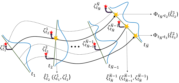
These considerations motivate the question of how to leverage the full set of samples and the system’s observability properties to construct a better ambiguity set at time $T$. If full-state samples were drawn from different realizations of the system at each $t_{i}$, they could be pushed forward through the flow map to obtain their corresponding values at $T$ and increase the exploitable data for the construction of the ambiguity set. Building on this observation, we address here three interconnected problems: (i) the dynamics transforms, and may potentially increase, the initial uncertainty about the random variable. It is therefore of interest to understand to what extent this may be compensated by the number of collected samples; (ii) bounded errors in the dynamics or, even if it is fully known, when the flow map cannot be computed exactly, induce errors in the propagation of the collected samples. It is therefore of interest to characterize accuracy versus horizon-length trade-offs; (iii) in the case of partial-state measurements, the issues (i) and (ii) need to be revisited to unveil how multiple output samples from each realization can be leveraged to recover the corresponding full state at time $T$.

II-B Fixed horizon dynamic DROP

We depart here from the static DROP paradigm and formulate the dynamic DROPs considered in this paper, where the data evolves according to the dynamics

$$\dot{\xi}_{t}=F(t,\xi_{t}),\qquad\xi_{t}\in\mathbb{R}^{d},$$ (1)

and is measured through the output map

$$\zeta_{t}=H(t,\xi_{t}),\qquad\zeta_{t}\in\mathbb{R}^{m}.$$ (2)

The initial condition $\xi_{0}$ is considered random with an unknown distribution $P_{\xi_{0}}$. Based on the evolution of (1) over an horizon $T$, we are interested in solving a DROP with respect to the unknown distribution $P_{\xi_{T}}$. As in Section II-A, cf. Figure 1, the samples are assumed to be gathered from independent realizations of the system. Because of the partial measurements, we make the following hypothesis on how trajectories are sampled.

Assumption II.1

(Sampling schedule). The data are gathered from $\bar{N}$ independent trajectories of (1) over the horizon $[0,T]$, denoted by $\xi^{i}$, $i=1,\ldots,\bar{N}$, having i.i.d. initial conditions $\xi_{0}^{i}$. From each trajectory $\xi^{i}$ we collect $\ell$ output samples $\zeta_{t_{i}^{l}}^{i}=H(t_{i}^{l},\xi_{t_{i}^{l}}^{i})$, at $t_{i}^{l}$, $l\in[1:\ell]$, with $0\leq t_{i}^{1}<\ldots<t_{i}^{\ell}\leq T$ and assume that $0\leq t_{1}^{\ell}\leq\cdots\leq t_{\bar{N}}^{\ell}=T$. We also denote $t_{i}^{\ell}\equiv t_{i}$, and, if $H(t,\xi)\equiv\xi$, we take $\ell=1$.

The assumption is motivated by scenarios where the trajectories’ outputs can be measured for a restricted amount of time. That can happen for instance when measurements are taken by a limited-range sensor, due to the fact that the location of the sensor and/or the random variable’s realizations changes with time (cf. Section VI). Figure 2 illustrates the sampling times associated to Assumption II.1. We refer to $\ell$, which represents a sufficient number of output samples to reconstruct the full state of a trajectory, as the observation horizon length. The hypothesis that $\ell$ is common for all trajectories is made without loss of generality, since we can otherwise take into account only the ones from which at least $\ell$ samples are collected, and select the last $\ell$ of them. The same holds also for the assumption that $0\leq t_{1}^{\ell}\leq\cdots\leq t_{\bar{N}}^{\ell}=T$, which can be enforced by simply relabeling the trajectories.

Figure 2: Sampling times where data are collected from independent trajectories according to Assumption II.1. The green arrows depict the tightest inter-trajectory sampling-time bound $\Delta$ and intra-trajectory inter-sampling-time bound $\Delta^{\prime}$. The blue double-sided arrow illustrates the time span associated to the effective sampling horizon.

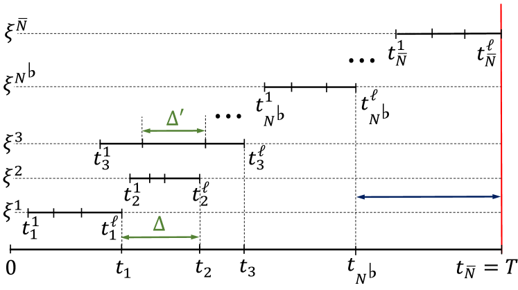
We call any $\Delta>0$ such that $\Delta\geq\max\{t_{i}-t_{i-1}\,|\,i\in[2:\bar{N}]\}$, an inter-trajectory sampling-time bound, and any $\Delta^{\prime}>0$ such that $\Delta^{\prime}\geq\max\{t_{i}^{l}-t_{i}^{l-1}\,|\,l\in[2:\ell],i\in[1:\bar{N}]\}$ an intra-trajectory inter-sampling-time bound. In addition, we introduce the effective sampling horizon $[N^{\flat}:\bar{N}]$, to indicate that the data used for the ambiguity set construction is collected from the trajectories $\xi^{N^{\flat}}$ up to $\xi^{\bar{N}}$, which we call effective trajectories (cf. Figure 2). The samples are exploited to estimate the state values of the $N:=\bar{N}-N^{\flat}+1$ effective trajectories at the horizon end $T$. The reason for considering this subset of trajectories is that it may not be desirable to use measurements from trajectories where the assimilation starts before $t_{N^{\flat}}$, due to the errors induced by the pushforward, which accumulate over time.

Problem statement: Given the horizon $[0,T]$, and under Assumption II.1, we seek to use each output tuple $(\zeta_{t_{i}^{1}}^{i},\ldots,\zeta_{t_{i}^{\ell}}^{i})$ to estimate the state $\widehat{\xi}_{t_{i}^{\ell}}^{i}$ of each effective trajectory $\xi^{i}$ at $t_{i}^{\ell}(\equiv t_{i})$, and determine an ambiguity set $\widehat{\mathcal{P}}_{T}^{N}$ containing the true distribution $P_{\xi_{T}}$ with high confidence. Under a fixed inter-trajectory sampling-time bound, we also seek to characterize the effect of the horizon length $T$ on the size of the constructed ambiguity set. Finally, in the presence of numerical errors or disturbances in the dynamics, we aim to quantify the effective horizon length up to which the ambiguity set is guaranteed to improve with the number of samples.

We start by addressing these problems for the case of full-state measurements, characterizing the properties of dynamic ambiguity sets first under perfect knowledge of the flow map in Section III and then studying data-assimilation versus precision trade-offs in the presence of computational errors in Section IV. Section V extends the results to the case when the random variable is only partially measured and evolves linearly.

III Ambiguity Sets Under Full-State Measurements

In this section, we characterize ambiguity sets that appear in dynamic DROPs, as described in the problem formulation of Section II-B, when full-state measurements $H(t,\xi)\equiv\xi$ are available. Thus, according to Assumption II.1, there is an increasing sequence of sampling times $0\leq t_{1}\leq\cdots\leq t_{\bar{N}}=T$, where at each $t_{i}$, the state sample $\xi_{t_{i}}^{i}$ is collected from a trajectory $\xi^{i}$ of (1), and the observation horizon is $\ell=1$. The ambiguity set $\widehat{\mathcal{P}}_{T}^{N}$ is built based on the $N=\bar{N}-N^{\flat}+1$ last effective samples by leveraging concentration of measure inequalities. For a moment, assume that $N$ independent samples $\xi_{T}^{i}$ become available at time $T$, and that a selected confidence $1-\beta>0$ is chosen. Thus, an ambiguity ball in $\mathcal{P}_{p}(\mathbb{R}^{d})$ can be constructed using the Wasserstein metric $W_{p}$ with center at the empirical distribution $\widehat{P}_{\xi_{T}}^{N}$ and radius $\varepsilon_{N}(\beta)$. It can be shown, cf. [13, Theorem 3.5], that the true distribution $P_{\xi_{T}}$ is in this ball with probability at least $1-\beta$, namely, $\mathbb{P}(W_{p}(\widehat{P}_{\xi_{T}}^{N},P_{\xi_{T}})\leq\varepsilon_{N}(\beta))\geq 1-\beta$. Recalling that in our setting the samples $\xi_{t_{i}}^{i}$, $i\in[N^{\flat}:\bar{N}]$ are to be collected progressively prior to $t_{\bar{N}}=T$, we alternatively seek to build the cumulative empirical distribution $\bar{P}_{\xi_{T}}^{N}$, using predicted values $\bar{\xi}_{T}^{i}$ of these samples at $T$.

More formally, consider a probability space $(\Omega,\mathcal{F},\mathbb{P})$ and a finite sequence of i.i.d. $\mathbb{R}^{d}$-valued random variables $(\xi_{0}^{i})_{i\in[1:\bar{N}]}$ with law $P_{\xi_{0}}\equiv P$, where each $\xi_{0}^{i}$ represents the initial condition of a trajectory $\xi^{i}$. The trajectories evolve according to the dynamics (1). From now on, we assume that $F$ in (1) is continuous and locally Lipschitz in $\xi$, and that the system is forward complete. Then, the flow map $\Phi:\mathcal{D}_{\Phi}\to\mathbb{R}^{d}$, where $\mathcal{D}_{\Phi}:=\{(t,s,\xi)\in\mathbb{R}_{\geq 0}\times\mathbb{R}_{\geq 0}\times\mathbb{R}^{d}:t\geq s\}$, is defined by $\Phi(t,s,\xi):=\xi_{t}(s,\xi)$, inducing a family of maps $\Phi_{t,s}:\mathbb{R}^{d}\to\mathbb{R}^{d}$. Assuming that all trajectories start at time $s=0$ and using the notation $\Phi_{t}=\Phi_{t,0}$, the state of each trajectory $\xi^{i}$ at time $t\geq 0$ is given by the random variable $\xi_{t}^{i}=\Phi_{t}\circ\xi_{0}^{i}$, with common law $P_{\xi_{t}}=\Phi_{t\#}P$. We next show that, under perfect knowledge of the flow map, the cumulative empirical distribution at $T$ formed by the predicted values $\bar{\xi}_{T}^{i}:=\Phi_{T,t_{i}}(\xi_{t_{i}}^{i})$, coincides with that of all the samples gathered at time $T$. The proof of the result is given in the Appendix.

Lemma III.1

(Ideal pushforward of sampled states). Consider a sequence of trajectories $\xi^{i}$ as in Assumption II.1, and the empirical distribution $\widehat{P}_{\xi_{T}}^{N}$ formed by the $N$ state samples of the effective trajectories $\xi^{N^{\flat}},\ldots,\xi^{\bar{N}}$ at $T$, i.e.,

$$\widehat{P}_{\xi_{T}}^{N}:=\frac{1}{N}\sum_{i=N^{\flat}}^{\bar{N}}\delta_{\xi_{T}^{i}}.$$ (3)

Then, (i) all $\xi_{T}^{i}$ are i.i.d., and (ii) if we consider the cumulative empirical distribution

$$\bar{P}_{\xi_{T}}^{N}:=\frac{1}{N}\sum_{i=N^{\flat}}^{\bar{N}}\delta_{\bar{\xi}_{T}^{i}},$$ (4)

with $\bar{\xi}_{T}^{i}=\Phi_{T,t_{i}}(\xi_{t_{i}}^{i})$, $i\in[N^{\flat}:\bar{N}]$, it holds that $\bar{P}_{\xi_{T}}^{N}=\widehat{P}_{\xi_{T}}^{N}$.

This result solves the issue of computing the evolving center of the ambiguity ball. We next turn our attention to determining its radius so as to ensure that the true distribution is contained in it with high confidence.

III-A Ambiguity radius for compactly supported distributions

We next present results from concentration of measure to determine the radius of the ambiguity set $\widehat{\mathcal{P}}_{T}^{N}$ that contains the true distribution $P_{\xi_{T}}$ of the data at $T$ with a selected confidence. Our focus is on the class of compactly supported distributions, which is preserved under the flow of forward complete systems. The following result provides a concentration inequality for such laws and its explicit dependence on the distribution’s support.

Proposition III.2

(Concentration inequality). Consider a sequence $(X_{i})_{i\in\mathbb{N}}$ of i.i.d. $\mathbb{R}^{d}$-valued random variables with a compactly supported law $\mu$. Then, for any $p\geq 1$, $N\geq 1$, and $\varepsilon>0$, it holds that

$$\mathbb{P}(W_{p}^{p}(\widehat{\mu}^{N},\mu)\geq\varepsilon)\leq\chi_{N}(\varepsilon,\rho;p,d),$$

$$\chi_{N}(\varepsilon,\rho):=C\begin{cases}e^{-\frac{cN}{\rho^{2p}}\varepsilon^{2}},&{\rm if}\;p>d/2,\\ e^{-cN\frac{\varepsilon^{2}}{\rho^{2p}(\ln(2+\rho^{p}/\varepsilon))^{2}}},&{\rm if}\;p=d/2,\\ e^{-\frac{cN}{\rho^{d}}\varepsilon^{\frac{d}{p}}},&{\rm if}\;p<d/2,\end{cases}$$ (5)

where $\widehat{\mu}^{N}:=\frac{1}{N}\sum_{i=1}^{N}\delta_{X_{i}}$, $\rho:=\frac{1}{2}\operatorname{diam}({\rm supp}(\mu))$, and the constants $C$ and $c$ depend only on $p$ and $d$.

Proof:

We employ the following fact, which can be found in [30, Proposition 7.16] and [12, Lemma 1].

$\triangleright$ Fact I. Let $T:\mathbb{R}^{d}\to\mathbb{R}^{d}$ with $T(x)=\bar{x}+Lx$ for all $x\in\mathbb{R}^{d}$, where $\bar{x}\in\mathbb{R}^{d}$ and $L>0$. Then, for any $\mu,\nu\in\mathcal{P}_{p}(\mathbb{R}^{d})$ it holds that $LW_{p}(\mu,\nu)=W_{p}(T_{\#}\mu,T_{\#}\nu)$. $\triangleleft$

Let $z\in\mathbb{R}^{d}$ with $\|x-z\|_{\infty}\leq\rho$ for all $x\in{\rm supp}(\mu)$ and consider the mapping $y=T(x):=\frac{x-z}{\rho}$ and the random variables $Y_{i}=T(X_{i})$, $i\in\mathbb{N}$, with law $\mu_{Y}=T_{\#}\mu$. Then, the $Y_{i}$’s are also i.i.d. and without loss of generality they are considered supported precisely on $(-1,1]^{d}$. We claim that

$$\{W_{p}^{p}(\widehat{\mu}^{N}_{Y},\mu_{Y})\geq\varepsilon\}=\{W_{p}^{p}(\widehat{\mu}^{N},\mu)\geq\rho^{p}\varepsilon\},$$ (6)

where $\widehat{\mu}_{Y}^{N}=\sum_{i=1}^{N}\delta_{Y_{i}}$. Indeed, let $\omega\in\Omega$. Then, we have that $Y_{i}(\omega)=T(X_{i}(\omega))$ for all $i$ and using the properties of the pushforward map, we get

$$T_{\#}\widehat{\mu}^{N}(\omega) =T_{\#}\frac{1}{N}\sum_{i=1}^{N}\delta_{X_{i}(\omega)}=\frac{1}{N}\sum_{i=1}^{N}T_{\#}\delta_{X_{i}(\omega)}$$

$$=\frac{1}{N}\sum_{i=1}^{N}\delta_{T(X_{i}(\omega))}=\frac{1}{N}\sum_{i=1}^{N}\delta_{Y_{i}(\omega)}=\widehat{\mu}^{N}_{Y}(\omega).$$

Taking also into account that $T_{\#}\mu=\mu_{Y}$, and exploiting Fact I with $\bar{x}=-\frac{z}{\rho}$ and $L=\frac{1}{\rho}$, it follows that $W_{p}(\widehat{\mu}^{N},\mu)=\rho W_{p}(\widehat{\mu}^{N}_{Y},\mu_{Y})$, and we conclude that (6) holds. In order to derive the desired inequality, we will use the following result:

$\triangleright$ [14, Proposition 10] Consider a sequence $(Z_{i})_{i\in\mathbb{N}}$ of i.i.d. $\mathbb{R}^{d}$-valued random variables with law $\nu$, supported on $(-1,1]^{d}$. Then, for any $p\geq 1$, $N\geq 1$, and $\varepsilon>0$, it holds that $\mathbb{P}(W_{p}^{p}(\widehat{\nu}^{N},\nu)\geq\varepsilon)\leq\chi_{N}(\varepsilon,1)$, where $\widehat{\nu}^{N}:=\frac{1}{N}\sum_{i=1}^{N}\delta_{Z_{i}}$, $C$ and $c$ depend only on $p$ and $d$, and $\chi_{N}$ is given in (5). $\triangleleft$

By applying this result with $\nu=\mu_{Y}$ and $\widehat{\nu}^{N}=\widehat{\mu}_{Y}^{N}$ to bound $\mathbb{P}(W_{p}^{p}(\widehat{\mu}^{N}_{Y},\mu_{Y})\geq\varepsilon)$ and substituting the right-hand side of (6) in this probability, we obtain the desired result. ∎

The following corollary to Proposition III.2 characterizes the radius of the ambiguity balls in terms of the selected confidence and the support of the unknown distribution.

Corollary III.3

(Ambiguity radius). Under the assumptions of Proposition III.2, for any confidence $1-\beta$, $\beta\in(0,1)$, it holds that $\mathbb{P}(W_{p}(\widehat{\mu}^{N},\mu)\leq\varepsilon_{N}(\beta,\rho))\geq 1-\beta$, where

$$\varepsilon_{N}(\beta,\rho):=\begin{cases}\left(\frac{\ln(C\beta^{-1})}{c}\right)^{\frac{1}{2p}}\frac{\rho}{N^{\frac{1}{2p}}},&{\rm if}\;p>d/2,\\ h^{-1}\left(\frac{\ln(C\beta^{-1})}{cN}\right)^{\frac{1}{p}}\rho,&{\rm if}\;p=d/2,\\ \left(\frac{\ln(C\beta^{-1})}{c}\right)^{\frac{1}{d}}\frac{\rho}{N^{\frac{1}{d}}},&{\rm if}\;p<d/2,\end{cases}$$ (7)

with $h^{-1}$ the inverse of $h(x)=\frac{x^{2}}{(\ln(2+1/x))^{2}}$, $x>0$.

III-B Growth conditions for ambiguity radius convergence

Here, we present sufficient conditions on the system’s dynamics and the sampling rate to guarantee that, for any prescribed confidence $1-\beta$, the radius of the ambiguity balls converges to zero as the horizon $[0,T]$ grows. We start with a Lyapunov-type characterization of the growth rate of the system dynamics.

Proposition III.4

(Lyapunov-type growth rate condition). For system (1), assume that there exist a locally integrable function $\alpha:\mathbb{R}_{\geq 0}\to\mathbb{R}$, and a function $V\in C^{1}(\mathbb{R}^{d};\mathbb{R})$, with

$$a_{1}\|\xi\|^{r}\leq V(\xi)\leq a_{2}\|\xi\|^{r},\quad\forall\xi\in\mathbb{R}^{d},$$ (8a)

$$DV(\xi)F(t,\xi)\leq \alpha(t)V(\xi)+M_{1}V(\xi)^{q},$$

$$\hskip 50.00008pt\forall t\geq 0,\xi\in\mathbb{R}^{d}\setminus\{0\},$$ (8b)

for certain $a_{1},a_{2}>0$, $r>1$, $M_{1}\geq 0$, and $q\in(-\infty,1)$. Then, for any initial condition $\xi_{0}\in\mathbb{R}^{d}$: (i) if $M_{1}=0$, then

$$\|\xi(t)\|\leq(a_{2}/a_{1})^{\frac{1}{r}}\|\xi_{0}\|e^{\frac{1}{r}\int_{0}^{t}\alpha(s)ds},\quad\forall t\geq 0;$$ (9)

(ii) if $M_{1}>0$, and additionally

$$\int_{t_{1}}^{t_{2}}\alpha(t)dt\leq M_{2},\quad\forall\;t_{2}\geq t_{1}\geq 0,$$ (10)

for certain $M_{2}>0$, then

$$\|\xi(t)\|\leq\bar{M}(1+\bar{c}t)^{\frac{1}{r(1-q)}},\quad\forall t\geq 0,$$ (11)

with

$$\bar{M}:=(e^{M_{2}}(1+a_{2}\|\xi_{0}\|^{r})/a_{1})^{\frac{1}{r}},\quad\bar{c}:=M_{1}(1-q).$$ (12)

The proof of Proposition III.4 is given in the Appendix. Next, we provide the main result of this section, which shows that for bounded inter-sampling times and under the assumption that full-state measurements are gathered and pushed without errors forward in time, the ambiguity sets formed by dynamics which satisfy the growth conditions of Proposition III.4 shrink as the DROP’s horizon increases.

Proposition III.5

(Ambiguity radius convergence). Assume that system (1) satisfies the assumptions of Proposition III.4 and that $P_{\xi_{0}}$ is supported on the compact set $K$. Select a confidence $1-\beta$, an exponent $p\geq 1$, and assume that

$$M_{1}>0,\quad r(1-q)>\max\{2p,d\},$$ (13a)

where $$r,q,M_{1}$$ are given in Proposition III.4, or that

$$M_{1}=0,\quad rq^{\prime}>\max\{2p,d\},\quad\int_{0}^{t}\alpha(s)ds\leq\frac{\ln t}{q^{\prime}},\forall t\geq t_{0}$$ (13b)

for some $q^{\prime}>0$ and $t_{0}>0$. For any horizon $[0,T]$, consider a sampling sequence as in Assumption II.1, with $t_{1}=0$ and inter-trajectory sampling-time bound independent of $T$, and let

$$\rho_{T}:=\operatorname{diam}(\Phi_{T}(K))/2,$$ (14)

with $\Phi_{T}(K)$ the set of reachable states at $T$ from $K$. Then,

$$P(W_{p}(\bar{P}_{\xi_{T}}^{N},P_{\xi_{T}})\leq\varepsilon_{N}({\beta},\rho_{T})) \geq 1-\beta,$$ (15a)

$$\lim_{T\to\infty}\varepsilon_{N}({\beta},\rho_{T}) =0,$$ (15b)

where $\varepsilon_{N}$ is given in (7) and $\bar{P}_{\xi_{T}}^{N}$ is the cumulative empirical distribution in (4), with $N^{\flat}=1$ and $N=\bar{N}$.

Proof:

We will leverage the results of Lemma III.1, Corollary III.3, and Proposition III.4 for the proof. Note first that, under perfect knowledge of the flow map, it follows from Lemma III.1(ii) that the center $\bar{P}_{\xi_{T}}^{N}$ of the ambiguity ball in (15a) is the same as $\widehat{P}_{\xi_{T}}^{N}$, i.e., the empirical distribution formed by $N$ samples $\xi_{T}^{1},\ldots,\xi_{T}^{N}$ of independent trajectories at $T$. Due to Lemma III.1(i), these samples are i.i.d.. Thus, we can apply Corollary III.3 to the empirical distribution $\widehat{\mu}^{N}=\widehat{P}_{\xi_{T}}^{N}=\bar{P}_{\xi_{T}}^{N}$ to infer that $\mathbb{P}(W_{p}(\bar{P}_{\xi_{T}}^{N},P_{\xi_{T}})\leq\varepsilon_{N}(\beta,\rho_{T}))\geq 1-\beta$ holds, or, in other words, (15a).

Next, note that since $K$ is compact, there is some $\rho>0$ with $K\subset\{\xi\in\mathbb{R}^{d}:\|\xi\|_{\infty}\leq\rho\}$. Thus, when (13a) is fulfilled, it follows from Proposition III.4 that

$$\rho_{T}\leq\bar{M}(1+\bar{c}T)^{\frac{1}{r(1-q)}},$$ (16)

where $\bar{c}$ and $\bar{M}$ are given by (12) with $\|\xi_{0}\|$ in the definition of $\bar{M}$ replaced by $\sqrt{d}\rho$. Next, define $i(T):={\lfloor T/\Delta\rfloor}+1$, where $\Delta$ is a common inter-trajectory sampling-time bound for each horizon $[0,T]$. Note that $i(T)\leq N$ and $T<\Delta i(T)$, implying by (16) that

$$\rho_{T}<\bar{M}(1+\bar{c}\Delta i(T))^{\frac{1}{r(1-q)}}=:\bar{\rho}_{T}.$$

From the latter, (7), the fact that $i(T)\leq N$, and that $\varepsilon_{N}(\beta,\rho_{T})$ decreases with $N$ and increases with $\rho_{T}$, it follows that

$$\varepsilon_{N}(\beta,\rho_{T})<\varepsilon_{i(T)}(\beta,\bar{\rho}_{T})$$

$$=\begin{cases}\left(\frac{\ln(C\beta^{-1})}{c}\right)^{\frac{1}{2p}}\frac{\bar{M}(1+\bar{c}\Delta i(T))^{\frac{1}{r(1-q)}}}{i(T)^{\frac{1}{2p}}},&{\rm if}\;p>d/2,\\ h^{-1}\left(\frac{\ln(C\beta^{-1})}{ci(T)}\right)^{\frac{1}{p}}\bar{M}(1+\bar{c}\Delta i(T))^{\frac{1}{r(1-q)}},&{\rm if}\;p=d/2,\\ \left(\frac{\ln(C\beta^{-1})}{c}\right)^{\frac{1}{d}}\frac{\bar{M}(1+\bar{c}\Delta i(T))^{\frac{1}{r(1-q)}}}{i(T)^{\frac{1}{d}}}&{\rm if}\;p<d/2.\end{cases}$$

Thus, it suffices to show that $\lim_{T\to\infty}\varepsilon_{i(T)}(\beta,\bar{\rho}_{T})=0$. In particular, when $p\neq d/2$, by setting $\bar{p}=\max\{2p,d\}$, we get

$$\lim_{T\to\infty}\varepsilon_{i(T)}(\beta,\bar{\rho}_{T}) =\lim_{T\to\infty}\frac{C^{\prime}(1+\bar{c}\Delta i(T))^{\frac{1}{r(1-q)}}}{i(T)^{\frac{1}{\bar{p}}}}$$

$$\leq\lim_{T\to\infty}C^{\prime\prime}i(T)^{\frac{\bar{p}-r(1-q)}{\bar{p}r(1-q)}}=0,$$

because of (13a) and the fact that $i(T)\to\infty$ when $T\to\infty$, where the constants $C^{\prime}$ and $C^{\prime\prime}$ in the derivation are independent of $T$. For the case where $p=d/2$, the result follows analogously by exploiting the following technical fact whose proof is given in the Appendix.

$\triangleright$ Fact II. For any $\bar{q}>2$ and $a>0$, it holds that $\lim_{\kappa\to\infty}h^{-1}(a/\kappa)\kappa^{\frac{1}{\bar{q}}}=0$, with $h$ given in Corollary III.3. $\triangleleft$

Finally, when (13b) holds, we obtain form (9) that

$$\|\xi(t)\|\leq(a_{2}/a_{1})^{\frac{1}{r}}\|\xi_{0}\|e^{\frac{1}{rq^{\prime}}\ln t},$$

for all $t\geq t_{0}$, and thus, that there exists a constant $\bar{M}^{\prime}$ with $\rho_{T}\leq\bar{M}^{\prime}(1+T)^{\frac{1}{rq^{\prime}}}$ for all $T>0$. Then, the result follows by using precisely the same arguments as before. ∎

IV Ambiguity Sets under Pushforward Errors and Disturbances

In general, the dynamics (1) of the random variable cannot be solved for explicitly. The pushforward of full-state samples hence requires the numerical integration of the system’s solutions, which gives rise to an approximation $\Phi^{\textup{num}}$ of the exact flow map. In addition, the dynamics of the process may be subject to disturbances. Both cases suggest that the cumulative empirical distribution $\bar{P}_{\xi_{T}}^{N}$ in (4) will no longer coincide with the empirical distribution $\widehat{P}_{\xi_{T}}^{N}$ in (3). We proceed to quantify this difference and characterize the relevant ambiguity sets, focusing first on the case where the flow is numerically integrated. Recall that the dynamics is continuous and locally Lipschitz. It therefore follows from classical approaches to bound the numerical integration error [29, Theorem 3.4.7], that for any compact set $K\subset\mathbb{R}^{n}$ and finite time horizon $[0,T]$, there exist positive constants $\mathfrak{K}$ and $L$, such that

$$\|\Phi^{\textup{num}}_{t,s}(\xi)-\Phi_{t,s}(\xi)\|\leq\mathfrak{K}(e^{L(t-s)}-1),$$ (17)

for all $0\leq s\leq t\leq T$ and $\xi\in\Phi_{s}(K)$. For the center of the ambiguity ball containing $P_{\xi_{T}}$, we consider a variant of the cumulative empirical distribution $\bar{P}_{\xi_{T}}^{N}$ in (4), formed by pushing forward the full-state samples by $\Phi^{\textup{num}}$. The following result, whose proof is in the Appendix, specifies the radius of the ambiguity set at the end of the horizon.

Theorem IV.1

(Ambiguity radius with approximate pushforward). Assume that the support of the initial condition of system (1) is contained in the compact set $K$. Consider a sampling sequence as in Assumption II.1 with inter-trajectory sampling-time bound $\Delta>0$, and the cumulative empirical distribution $\bar{P}_{\xi_{T}}^{N}$ in (4), with $\bar{\xi}_{T}^{i}:=\Phi^{\textup{num}}_{T,t_{i}}(\xi_{t_{i}}^{i})$, $i\in[N^{\flat}:\bar{N}]$. Then, for any confidence $1-\beta$ and $p\geq 1$ it holds

$$\mathbb{P}(W_{p}(\bar{P}_{\xi_{T}}^{N},P_{\xi_{T}}) \leq\psi_{N}(\beta,\Delta))\geq 1-\beta,$$ (18a)

where

$$\psi_{N}(\beta,\Delta): =\varepsilon_{N}(\beta,\rho_{T})+\bar{\varepsilon}_{N}(\Delta),$$ (18b)

$$\bar{\varepsilon}_{N}(\Delta): =\mathfrak{K}\Big{(}\frac{1}{N}\int_{1}^{N}(e^{L\Delta s}-1)^{p}ds\Big{)}^{\frac{1}{p}},$$ (18c)

with $\varepsilon_{N}(\beta,\rho_{T})$ and $\rho_{T}$, as given in (7) and (14), respectively.

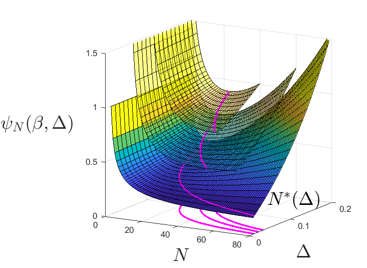
According to this result, when the exact flow map is no longer available, the ambiguity radius needs to be increased with the additional term $\bar{\varepsilon}_{N}$ to obtain the same high-confidence guarantee. In the ideal case where $\mathfrak{K}=0$ in (18c), we recover the result of Corollary III.3. The extra term $\bar{\varepsilon}_{N}$ increases as we consider more samples, since they are located farther back in time and pushing them forward induces larger errors. Based on Theorem IV.1 we quantify the effective sampling horizon size in terms of guaranteed ambiguity reduction in the presence of numerical errors.

Proposition IV.2

(Effective sampling horizon). Under the hypotheses of Theorem IV.1, assume additionally that $p\neq d/2$. Let $\bar{p}:=\max\{2p,d\}$ and $\bar{C}\equiv\bar{C}(\bar{p},\beta,\rho_{T}):=\Big{(}\frac{\ln(C\beta^{-1})}{c}\Big{)}^{\frac{1}{\bar{p}}}\rho_{T}$, with $C$, $c$ and $\rho_{T}$ as in (7) and (14), respectively. Then, there exists $\Delta^{*}\equiv\Delta^{*}(\bar{C},L,\mathfrak{K})>0$ such that for every $\Delta\in(0,\Delta^{*})$, the set

$$\mathcal{N}(\Delta):=\{N\in\mathbb{N}\,|\,\bar{C}( \kappa^{-\frac{1}{\bar{p}}}-(\kappa+1)^{-\frac{1}{\bar{p}}})$$

$$>\bar{\varepsilon}_{\kappa+1}(\Delta)-\bar{\varepsilon}_{\kappa}(\Delta),\,\forall\kappa\in[1:N]\},$$

with $\bar{\varepsilon}_{1},\ldots,\bar{\varepsilon}_{N+1}$ as given in (18c), is nonempty and bounded. In addition, the ambiguity radius $\psi_{N}(\beta,\Delta)$ in (18b) is strictly decreasing with $N$, for $N\in[1:N^{*}(\Delta)]$, with $N^{*}(\Delta):=\max(\mathcal{N}(\Delta))+1$.

Proof:

From (18c), we get that $\lim_{\Delta\to 0}\bar{\varepsilon}_{N}(\Delta)=0$ for all $N\in\mathbb{N}$. Thus, there exists $\Delta^{*}>0$ such that $\bar{\varepsilon}_{2}(\Delta)-\bar{\varepsilon}_{1}(\Delta)<\bar{C}(1-2^{-\frac{1}{\bar{p}}})$ for all $\Delta<\Delta^{*}$, implying that $1\in\mathcal{N}(\Delta)$, and hence, that $\mathcal{N}(\Delta)$ is nonempty. In addition, we have that $\lim_{N\to\infty}\bar{\varepsilon}_{N}(\Delta)=\infty$ for all $p\geq 1$, which implies that $\mathcal{N}(\Delta)$ is bounded. Indeed, otherwise it would hold that

$$\bar{\varepsilon}_{N+1}(\Delta)-\bar{\varepsilon}_{1}(\Delta)=\sum_{\kappa=1}^{N}(\bar{\varepsilon}_{\kappa+1}(\Delta)-\bar{\varepsilon}_{\kappa}(\Delta))$$

$$<\sum_{\kappa=1}^{N}\bar{C}(\kappa^{-\frac{1}{\bar{p}}}-(\kappa+1)^{-\frac{1}{\bar{p}}})=\bar{C}(1-(N+1)^{-\frac{1}{\bar{p}}})<\bar{C}$$

for all $N\in\mathbb{N}$, leading to a contradiction. Thus $N^{*}(\Delta)$ is always finite. Furthermore, from (7), (18b), and the definition of $\bar{C}$, $N^{*}(\Delta)$, and $\mathcal{N}(\Delta)$, we get $\psi_{N+1}(\beta,\Delta)<\psi_{N}(\beta,\Delta)$ for all $N\in[1:N^{*}(\Delta)-1]$, as desired. ∎

Proposition IV.2 identifies the upper bound $N^{*}(\Delta)$ on the number of samples below which one can guarantee that the more samples the better regarding the ambiguity radius. Figure 3 illustrates how the ambiguity radius $\psi_{N}(\beta,\Delta)$ in (18b) varies with respect to the sampling period and the number of samples in the presence of numerical errors.

Figure 3: (a) shows how the ambiguity radius $\psi_{N}(\beta,\Delta)$ in (18b) varies with respect to $\Delta$ and $N$ for a fixed confidence $1-\beta$, and the parameter values $d=1$, $p=1$, $L=0.1$, $\mathfrak{K}=1$, and $\rho_{T}\in\{1,2,3\}$. Given that the component $\varepsilon_{N}$ of the radius, which is strictly decreasing with $N$, is proportional to the distributions’ support size and that the effect of numerical errors is independent of $\rho_{T}$, the effective sampling horizon increases with $\rho_{T}$, as shown in (b).

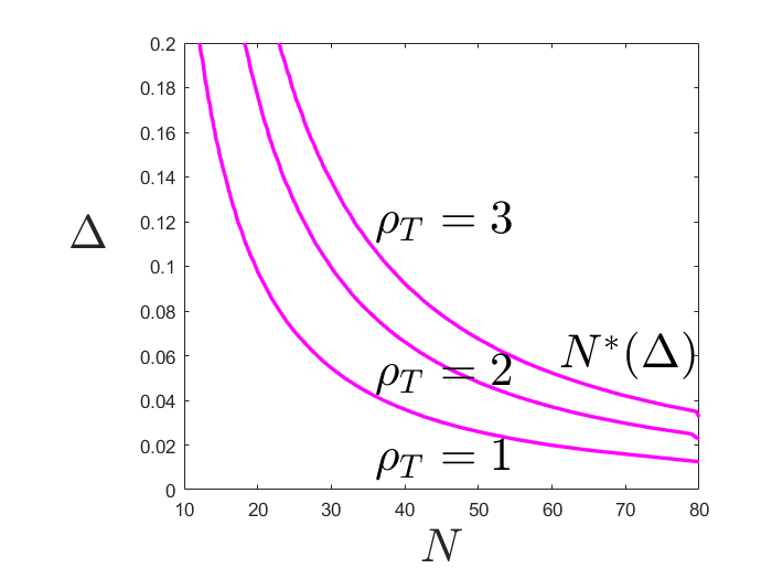
Theorem IV.1 and Proposition IV.2 are also applicable when the sampled trajectories are subject to unknown disturbances $\mathfrak{d}$. Formally, the dynamics in this case takes the form

$$\dot{\xi_{t}}=F(t,\xi_{t},\mathfrak{d}_{t}),$$

where $\mathfrak{d}$ belongs to a class $\mathcal{D}$ of functions, which are uniformly bounded for every finite time horizon, and with $\mathfrak{d}\equiv 0$ being an element of $\mathcal{D}$. Additionally, we assume that $F$ is also locally Lipschitz with respect to its $\mathfrak{d}$ argument. For any constant $\varepsilon>0$ and horizon $[0,T]$, let $B:=\{\Phi_{t}(\xi)\,|\,\xi\in K,t\in[0,T]\}$ and $B_{\varepsilon}:=\{\xi\in\mathbb{R}^{d}\,|\,\operatorname{dist}(\xi,B)\leq\varepsilon\}$, where $K$ is a compact set containing the initial state $\xi_{0}$. Using the local Lipschitzness assumption, we can select a constant $L>0$ so that

$$\|F(t,\xi,\mathfrak{d}_{t})-F(t,\xi^{\prime},\mathfrak{d}_{t}^{\prime})\|\leq L\|(\xi,\mathfrak{d}_{t})-(\xi^{\prime},\mathfrak{d}_{t}^{\prime})\|,$$

for all $t\in[0,T]$, $\xi,\xi^{\prime}\in B_{\varepsilon}$ and $\mathfrak{d},\mathfrak{d}^{\prime}\in\mathcal{D}$. Then, from [18, Theorem 3.4], it follows that (17) holds with $\Phi^{\textup{num}}_{t,s}$ replaced by the flow of $\dot{\xi_{t}}=F(t,\xi_{t},\mathfrak{d}_{t})$ and $\mathfrak{K}:=\min\{\sup_{t\in[0,T],\mathfrak{d}\in\mathcal{D}}\mathfrak{d}_{t},\frac{\varepsilon}{e^{LT}-1}\}$, for all disturbances $\mathfrak{d}\in\mathcal{D}$ with $\max_{t\in[0,T]}\mathfrak{d}_{t}\leq\mathfrak{K}$. With this bound in place, the proofs of Theorem IV.1 and Proposition IV.2 also hold for the case with disturbances.

V Ambiguity Sets for Partially Observable Linear Systems

Here we consider the case of partial measurements, where multiple samples are collected from each independent trajectory. We restrict our attention to linear time-varying systems with linear outputs, i.e.,

$$\dot{\xi}_{t}=A(t)\xi_{t},\quad\zeta_{t}=C(t)\xi_{t},$$ (19)

with $A(t)\in\mathbb{R}^{d\times d}$ and $C(t)\in\mathbb{R}^{m\times d}$. In this case, the full state of each trajectory $\xi^{i}$ is no longer directly available through the individual output samples. However, it is possible to recover it when the system is sampled-data observable, and combine this knowledge with our approach in the previous sections to build the ambiguity sets. We therefore start by examining observability conditions under which the state reconstruction is possible when a sufficient number of output samples is collected.

V-A Sampled data observability

For the linear time-varying system (19), let $\Phi(t,s)\in\mathbb{R}^{d\times d}$, for $t,s\geq 0$, denote its fundamental matrix, satisfying $\Phi_{t,s}(\xi)=\Phi(t,s)\xi$ for all $\xi\in\mathbb{R}^{d}$. According to Assumption II.1, we have $\ell$ output samples from each trajectory $\xi^{i}$. Each such sample can be evaluated as $\zeta_{t_{i}^{l}}^{i}=C(t_{i}^{l})\Phi(t_{i}^{l},t_{i}^{\ell})\xi_{t_{i}^{\ell}}^{i}$, $l\in[1:\ell]$, by taking the state at $t_{i}^{\ell}$ backward to time $t_{i}^{l}$ through the flow and computing its output value. Consequently, recovering the unmeasured state $\xi_{t_{i}^{\ell}}^{i}$ at the last sampling instant is equivalent to requiring that the sample-observability matrix

$$\bm{\mathcal{O}}_{i}\equiv\bm{\mathcal{O}}_{t_{i}^{1}\cdots t_{i}^{\ell}}^{\exp-}:=\left(\begin{matrix}C(t_{i}^{1})\Phi(t_{i}^{1},t_{i}^{\ell})\\ C(t_{i}^{2})\Phi(t_{i}^{2},t_{i}^{\ell})\\ \vdots\\ C(t_{i}^{\ell})\end{matrix}\right),$$ (20)

is left invertible. This turns out to hold when system (19) is sampled data observable and the observation horizon length $\ell$ is sufficiently large. We next present such sampled-data observability results, starting with the case when the system is (linear) time-invariant (LTI), i.e., $A(t)\equiv A$ and $C(t)\equiv C$.

Assumption V.1

The pair $(A,C)$ is observable and the sampling schedule satisfies either one of the following hypotheses:

H1 (Equidistant sampling). The sampling times are given by $t_{i}^{l}=t_{i}^{1}+(l-1)\Delta^{\prime}$, $l\in[1:\ell]$, $i\in[1:\bar{N}]$, for some $\Delta^{\prime}>0$, with $\Delta^{\prime}(\lambda-\lambda^{\prime})\neq 2k\pi j$ for all $k\in\mathbb{Z}$ and distinct eigenvalues $\lambda$, $\lambda^{\prime}$ of $A$, and $\ell\geq d$ (denoting $j\equiv\sqrt{-1}\in\mathbb{C}$).

H2 (Periodic non-equidistant sampling). The sampling times are given by the pattern

$$t_{i}^{l}:=\begin{cases}t_{i}^{1}+(l-1)\Delta^{\prime},&l\in[1:\bar{d}+1],\\ t_{i}^{1}+\bar{d}\Delta^{\prime}+\Delta^{\prime\prime},&l=\bar{d}+2,\\ t_{i}^{l-(\bar{d}+1)}+\bar{d}\Delta^{\prime}+\Delta^{\prime\prime},&l\in[\bar{d}+3:\ell],\end{cases}$$

with $\Delta^{\prime},\Delta^{\prime\prime}>0$, $\Delta^{\prime}/\Delta^{\prime\prime}\notin\mathbb{Q}$, $\bar{d}\geq d$, and $\ell\geq(\bar{d}+1)d$.

H3 (Irregular sampling). The observation horizon length $\ell$ satisfies the lower bound

$$\ell>\mathfrak{m}-1+\tau\delta/(2\pi),$$

where $\delta:=\max_{1\leq j,j^{\prime}\leq q}\{\Im(\lambda_{j}^{\prime}-\lambda_{j})\}$, $\mathfrak{m}:=\sum_{j=1}^{q}\mathfrak{m}_{j}$, $\tau:=\max\{t_{i}^{\ell}-t_{i}^{1},{i\in[1:\bar{N}]}\}$, and $\mathfrak{m}_{1},\ldots,\mathfrak{m}_{q}$ are the indices of $A$’s eigenvalues $\lambda_{1},\ldots,\lambda_{q}$.

The first sampling hypothesis in Assumption V.1 is a classical result, commonly known as the Kalman-Ho-Narendra criterion (see e.g., [28]). The second hypothesis is given in [20], whereas the last observability criterion under irregular sampling was originally presented in [31]. Here, we provide a slightly refined version of the latter from the more recent work [32, Theorem 2]. We next state formally that under either of the three cases for the sampling schedule, the sample observability matrix $\bm{\mathcal{O}}_{i}$ is left invertible. The proof of this result invokes classical arguments from LTI system theory. For completeness, since we found no verbatim statement in the literature, we provide a brief proof in the Appendix.

Lemma V.2

(Sampled-data observability for LTI systems). Assume that system (19) is LTI and that samples are collected according to Assumption II.1. Then, under the observability Assumption V.1, each matrix $\bm{\mathcal{O}}_{i}$ is left invertible.

Left invertibility of $\bm{\mathcal{O}}_{i}$ is equivalent to the property that its smallest singular value is strictly positive. However, the result of Lemma V.2 does not provide a bound on how far the smallest singular value lies from zero, or in other words, on the distance of the matrix from becoming singular. This distance is of particular interest when the collected output samples are perturbed.

We next provide conditions which guarantee robust invertibility of the sample-observability matrix by deriving uniform lower bounds for the smallest singular value of a weighted variant of $\bm{\mathcal{O}}_{i}$. These constitute a robust observability criterion under irregular sampling for the general time-varying case (19). We make the following assumption:

Assumption V.3

(Time-varying observability). System (19) is observable on any interval $[a,b]\subset[0,T]$, $t\mapsto A(t)$ is continuous, and $t\mapsto C(t)$ is continuously differentiable.

For each trajectory $\xi^{i}$, let $\tau(i):=t_{i}^{\ell}-t_{i}^{1}$ denote the length of the time interval during which output samples are collected. It holds that

$$0<\tau^{\textup{low}}:=\min_{i\in[1:\bar{N}]}\tau(i)\leq\tau(i)\leq\tau^{\textup{up}}:=\max_{i\in[1:\bar{N}]}\tau(i)\leq T,$$

for all $i\in[1:\bar{N}]$. Next, define

$$K(s,t):=\Phi(s,t)^{\top}C(s)^{\top}C(s)\Phi(s,t)$$ (21)

and

$$\mathcal{W}_{\varsigma}(t):=\int_{t}^{t+\varsigma}K(s,t+\varsigma)ds,$$ (22)

for $s,t,\varsigma\geq 0$. Then, $\mathcal{W}_{\varsigma}(t)=\Phi({t,t+\varsigma})^{\top}\widetilde{\mathcal{W}}_{\varsigma}(t)\Phi({t,t+\varsigma})$, where $\widetilde{\mathcal{W}}_{\varsigma}(t):=\int_{t}^{t+\varsigma}K(s,t)ds$ is the observability Gramian of (19) on $[t,t+\varsigma]$, which is continuous with respect to $t$. By Assumption V.3, the observability Gramian $\widetilde{\mathcal{W}}_{\tau^{\textup{low}}}(t)$ is also positive definite for all $t\in[0,T-\tau^{\textup{low}}]$ (see e.g., [28, Exercise 6.3.2]). Thus, the same properties hold for $\mathcal{W}_{\tau^{\textup{low}}}(t)$, implying

$$\lambda_{\min}\big{(}\mathcal{W}_{\tau^{\textup{low}}}(t)|_{0}^{T-\tau^{\textup{low}}}\big{)}:=\min_{t\in[0,T-\tau^{\textup{low}}]}\lambda_{\min}(\mathcal{W}_{\tau^{\textup{low}}}(t))>0,$$ (23)

where $\lambda_{\min}$ denotes smallest eigenvalue. Next, fix any $i\in[1:\bar{N}]$ and let

$${\tau_{l}(i)}:=t_{i}^{l+1}-t_{i}^{l},\;l\in[1:\ell-1],$$ (24)

be the lengths of the inter-sampling time intervals. Define the weight matrix

$$\bm{W}_{i} :=\operatorname{diag}(w_{1}(i),\ldots,w_{\ell}(i))\otimes I_{m},$$ (25)

$$\quad w_{1}^{2}(i)=\frac{\tau_{1}(i)}{2},\;w_{l}^{2}(i)=\frac{\tau_{l-1}(i)+\tau_{l}(i)}{2},$$

$$\hskip 33.99998ptl\in[2:\ell-1],\;w_{\ell}^{2}(i)=\frac{\tau_{\ell-1}(i)}{2}.$$

Next, we find a positive lower bound for the smallest eigenvalue of $\bm{\mathcal{O}}_{i}^{\top}\bm{W}_{i}\bm{W}_{i}\bm{\mathcal{O}}_{i}$. This fact implies the left invertibility of $\bm{\mathcal{O}}_{i}$. The proof of the result is given in the Appendix.

Proposition V.4

(Robust sampled-data observability). Under Assumption V.3, for $a\in(0,1)$, assume the intra-trajectory inter-sampling-time bound $\Delta^{\prime}$ satisfies

$$\Delta^{\prime}\leq\frac{4(1-a)\lambda_{\min}\big{(}\mathcal{W}_{\tau^{\textup{low}}}(t)|_{0}^{T-\tau^{\textup{low}}}\big{)}}{\tau^{\textup{up}}\max_{\tau^{\textup{low}}\leq t\leq T,\max\{0,t-\tau^{\textup{up}}\}\leq s\leq t}\|K_{s}(s,t)\|},$$ (26)

where $K_{s}(s,t):=\frac{\partial}{\partial s}K(s,t)$. Then, the system is sampled-data observable, i.e., for any $i\in[1:\bar{N}]$ the matrix $\bm{\mathcal{O}}_{i}$ is invertible. In addition,

$$\lambda_{\min}(\bm{\mathcal{O}}^{\top}_{i}\bm{W}_{i}\bm{W}_{i}\bm{\mathcal{O}}_{i})\geq a\lambda_{\min}\big{(}\mathcal{W}_{\tau^{\textup{low}}}(t)|_{0}^{T-\tau^{\textup{low}}}\big{)}.$$ (27)

We employ the bound in Proposition V.4 to quantify the state reconstruction error under perturbed measurements in the next section. The result of Proposition V.4 takes a more explicit form for LTI systems. In this case, note that $K(s,t)=\widehat{K}(s-t)$, with

$$\widehat{K}(t):=e^{A^{\top}t}C^{\top}Ce^{At}.$$ (28)

Hence, $\widehat{\mathcal{W}}_{\varsigma}:=\mathcal{W}_{\varsigma}(t)=\int_{0}^{\varsigma}\widehat{K}(s-{\varsigma})ds$ is independent of $t$, and $\lambda_{\min}\big{(}\mathcal{W}_{\tau^{\textup{low}}}(t)|_{0}^{T-\tau^{\textup{low}}}\big{)}=\lambda_{\min}(\widehat{\mathcal{W}}_{\tau^{\textup{low}}})$.

Corollary V.5

(Robust sampled-data observability for LTI systems). Under the assumptions of Proposition V.4, when (19) is time-invariant and the intra-trajectory inter-sampling-time bound $\Delta^{\prime}$ satisfies

$$\Delta^{\prime}\leq\frac{2(1-a)\lambda_{\min}(\widehat{\mathcal{W}}_{\tau^{\textup{low}}})}{\tau^{\textup{up}}\max_{s\in[0,\tau^{\textup{up}}]}\|\widehat{K}(s-\tau^{\textup{up}})A\|},$$ (29)

the system is sampled-data observable and (27) holds.

V-B Ambiguity sets under exact and inexact observations

Here we exploit the sampled observability results to characterize dynamic ambiguity sets under progressively collected output measurements. The next result is the analogue of Lemma III.1 when (19) is sampled data observable and measurements are exact.

Lemma V.6

(Ideal pushforward of output-sample reconstructed states). Consider a sequence of trajectories $\xi^{i}$ as in Assumption II.1, the empirical distribution $\widehat{P}_{\xi_{T}}^{N}$ in (3), and the cumulative empirical distribution $\bar{P}_{\xi_{T}}^{N}$ given by (4), with

$$\bar{\xi}_{T}^{i}:={\Phi(T,t_{i}^{\ell})}\bm{\mathcal{O}}_{i}^{\dagger}\bm{\zeta}^{i},$$ (30)

for $i\in[N^{\flat}:\bar{N}]$, where $\bm{\zeta}^{i}:=(\zeta_{t_{i}^{1}}^{i},\dots,\zeta_{t_{i}^{\ell}}^{i})$. Assume that either (19) is time-invariant and Assumption V.1 or the hypotheses of Corollary V.5 hold, or that it is time-varying and the assumptions of Proposition V.4 hold. Then, $\bar{P}_{\xi_{T}}^{N}=\widehat{P}_{\xi_{T}}^{N}$.

Proof:

From the definition of $\widehat{P}_{\xi_{T}}^{N}$ and $\bar{P}_{\xi_{T}}^{N}$, the result follows if we establish that $\bar{\xi}_{T}^{i}=\xi_{T}^{i}$ for all $i\in[N^{\flat}:\bar{N}]$. For each of the possible cases, we get from either Lemma V.2, Proposition V.4, or Corollary V.5, that the matrices $\bm{\mathcal{O}}_{i}$ are left invertible, and hence, that $\bm{\mathcal{O}}_{i}^{\dagger}\bm{\zeta}^{i}=\xi_{t_{\ell}^{i}}^{i}$. Thus, we deduce that $\bar{\xi}_{T}^{i}:={\Phi(T,t_{i}^{\ell})}\xi_{t_{\ell}^{i}}^{i}=\xi_{T}^{i}$, as desired. ∎

It is also worth noting that the result of Lemma V.6 generalizes to the nonlinear case under the same arguments, provided that the map associating the system’s initial states to the output samples is invertible.

Corollary V.7

(Nonlinear pushforward of output-sample reconstructed states). Consider the nonlinear system (1)-(2) and a sequence of trajectories $\xi^{i}$ as in Assumption II.1, Assume that for each $i\in[N^{\flat}:\bar{N}]$, the map $\mathcal{H}_{i}:\Phi_{t_{i}^{\ell}}(K)\to\mathbb{R}^{\ell m}$,

$$\mathcal{H}_{i}(\xi):=(H(t_{i}^{1},\Phi_{t_{i}^{1},t_{i}^{\ell}}(\xi)),H(t_{i}^{2},\Phi_{t_{i}^{2},t_{i}^{\ell}}(\xi)),\ldots,H(t_{i}^{\ell},\xi))$$

is invertible on its image, where $\Phi_{t_{i}^{\ell}}(K)\subset\mathbb{R}^{d}$ and $K$ contains the support of the initial conditions’ distribution. Then, the result of Lemma V.6 remains valid with $\bar{\xi}_{T}^{i}:=\Phi_{T,t_{i}^{\ell}}(\mathcal{H}_{i}^{-1}(\bm{\zeta}^{i}))$.

Using Lemma V.6, we obtain the analogue of Proposition III.5 for system (19) when exact output samples are assimilated.

Corollary V.8

(Output-sample based ambiguity radius convergence). Under Assumption V.3, further assume that the intra-trajectory inter-sampling-time bound $\Delta^{\prime}$ satisfies (26) and consider the cumulative empirical distribution in (4), where $\bar{\xi}_{T}^{i}$ is given by (30) with $N^{\flat}=1$. Then, under the hypotheses of Proposition III.5, for any confidence $1-\beta$, the ambiguity radius $\varepsilon_{N}(\beta,\rho_{T})$ satisfies $\lim_{T\to\infty}\varepsilon_{N}(\beta,\rho_{T})=0$.

Based on the derived observability results, we also obtain bounds for the discrepancy between the estimated state from the measurements and the true state, when the output samples are subject to bounded observation errors.

Proposition V.9

(State estimation error under bounded observation errors). Under Assumption V.3, further assume that, for each state trajectory $\xi^{i}$, instead of the exact output samples $\bm{\zeta}^{i}$ in (30), we measure

$$\bm{\widehat{\zeta}}^{i}=\bm{\zeta}^{i}+\bm{\delta}^{i},$$ (31)

for some $\bm{\delta}^{i}=(\delta_{1}^{i},\dots,\delta_{\ell}^{i})$, with $\|\delta_{l}^{i}\|\leq\delta^{*}$, for $l\in[1:\ell]$. Also, assume that the intra-trajectory inter-sampling-time bound $\Delta^{\prime}$ satisfies (26), or (29) if the system is time-invariant. Then, the estimated state $\widehat{\xi}_{t_{i}^{\ell}}^{i}:={(\bm{W}_{i}\bm{\mathcal{O}}_{i})^{\dagger}\bm{W}_{i}}\widehat{\bm{\zeta}}^{i}$ satisfies

$$\|\widehat{\xi}_{t_{i}^{\ell}}^{i}-\xi_{t_{i}^{\ell}}^{i}\|\leq\varepsilon^{*}:=\sqrt{\frac{\tau^{\textup{up}}}{a\lambda_{\min}\big{(}\mathcal{W}_{\tau^{\textup{low}}}(t)|_{0}^{T-\tau^{\textup{low}}}\big{)}}}\delta^{*}.$$ (32)

The proof of Proposition V.9 is given in the Appendix. We next provide the analogue to Theorem IV.1, i.e., we determine the ambiguity radius obtained through the cumulative empirical distribution $\bar{P}_{\xi_{T}}^{N}$, by pushing forward the estimated states from the perturbed measurements through the numerical approximation of the flow. Note that since according to Assumption V.3 the map $t\mapsto A(t)$ is continuous, $\Phi^{\textup{num}}$ satisfies (17) for all $0\leq s\leq t\leq T$, for some $\mathfrak{K}>0$, and $L:=\max_{t\in[0,T]}\|A(t)\|$.

Theorem V.10

(Ambiguity radius with approximate pushforward and observation errors). Under Assumption V.3, let the initial condition of (19) be supported on the compact set $K$. Consider a sampling sequence as in Assumption II.1, with inter-trajectory sampling-time bound $\Delta>0$, and intra-trajectory inter-sampling-time bound $\Delta^{\prime}>0$. For each effective trajectory $\xi^{i}$, $i\in[N^{\flat}:\bar{N}]$, we measure the inexact samples $\widehat{\bm{\zeta}}^{i}$ in (31), and we consider the cumulative empirical distribution $\bar{P}_{\xi_{T}}^{N}$ in (4), with

$$\bar{\xi}_{T}^{i}:=\Phi^{\textup{num}}_{T,t_{i}^{\ell}}({(\bm{W}_{i}\bm{\mathcal{O}}_{i})^{\dagger}\bm{W}_{i}}\widehat{\bm{\zeta}}^{i}),$$

and $\bm{\mathcal{O}}_{i}$ given by (20) for all $i$. Then, for any confidence $1-\beta$ and $p\geq 1$, (18a) holds, with $\psi_{N}$ as in (18b), $\bar{\varepsilon}_{N}$ given by

$$\bar{\varepsilon}_{N}(\Delta):=\Big{(}\frac{2^{p-1}}{N}\Big{(}\frac{(\varepsilon^{*})^{p}}{pL\Delta}(e^{pL\Delta N}-1)$$

$$\hskip 80.00012pt+\mathfrak{K}^{p}\int_{1}^{N}(e^{L\Delta s}-1)^{p}ds\Big{)}\Big{)}^{\frac{1}{p}},$$ (33)

instead of (18c), and $\varepsilon^{*}$ given by (32).

The proof of this result is given in the Appendix. Under the hypothesis of Theorem V.10, the result of Proposition IV.2 remains valid with $\bar{\varepsilon}_{N}$ as given by (33).

VI Application to UAV Detection

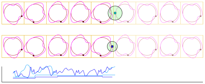
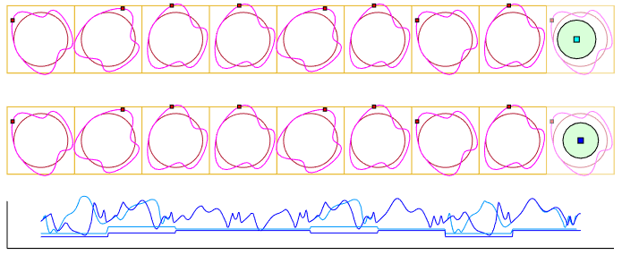
Here we illustrate our results in an application scenario involving a blue UAV that seeks to avoid detection while passing through an area surveilled by a team of red UAVs, cf. Figure 4.

Figure 4: (a) Red stars depict the location of red UAVs $A_{1},\ldots,A_{i},A_{i+1},\ldots$ at a specific time instant and the filled blue star depicts the location of the blue UAV $B$. Red circles represent the trajectories tracked by the red UAVs. The non-filled blue star represents the goal position of the blue UAV at the end of the optimization horizon, and the non-filled stars/dashed trajectories of the red UAVs with index $i+1$ and beyond signify that they have not been yet observed by the blue UAV. (b) shows the phase angle distribution of the reference trajectory tracked by red UAVs, which is unknown to the blue UAV.

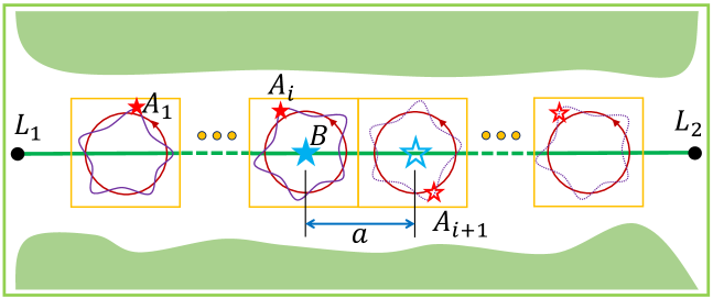
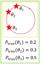
The red team has split the area into squares of identical size and assigned one UAV per square. With the vehicle’s coordinate system centered at the middle of the square, each red UAV tracks a circular orbit $\chi(t,\theta):=r(\cos(\theta+t),\sin(\theta+t))$ of radius $r$ according to the dynamics

$$\dot{\xi}_{1}(t) =\xi_{2}(t)$$

$$\dot{\xi}_{2}(t) =\kappa^{2}({\chi}(t,\theta)-\xi_{1}(t)).$$ (34)

Here, the phase angle $\theta$ is a parameter not known to the blue UAV that the red team selects randomly according to some distribution to make things harder for potential intruders. Note that this fits into the model (1) by setting $\dot{\theta}(t)=0$. The state of each UAV is $\xi=(\xi_{1},\xi_{2},\theta)\in\mathbb{R}^{5}$. The purpose of the blue UAV is to traverse the area along the straight path from location $L_{1}$ to location $L_{2}$ in Figure 4 while minimizing the possibility of being detected. The blue UAV is kinematic, actuating the magnitude of its velocity vector, which points from $L_{1}$ to $L_{2}$ and is upper bounded by $v_{\max}$ and lower bounded by $v_{\min}>0$, since it has not the ability to hover. The initial conditions of the red UAVs, i.e., initial position, velocity, and phase angle are independently sampled from a compactly supported distribution which is unknown to the blue UAV, except from its support. Thus, vehicle $B$ has no information about the state of each UAV $A_{i}$ before reaching region $i$.

DRO formulation

While traversing the corresponding square, the blue vehicle collects (at least three) exact position measurements from $A_{i}$ before reaching the center of the square. At the middle of each square $i$, the blue UAV solves an optimization problem to tune its velocity up to the center of the next region $i+1$ in order to simultaneously maximize the worst-case distance from UAV $A_{i}$, which has already been observed, and the worst-case expected distance from UAV $A_{i+1}$, based on the collected data of the preceding UAVs’ locations. This maximization is carried out during the traversal between the centers of squares $i$ and $i+1$, which are at a distance $a$ apart, and must be performed in $2\pi$ time units (the surveillance period of the red UAVs). For the purpose of the optimization, we divide $[0,2\pi]$ into $n$ equal subintervals so that, at time ${T_{i}}=i\cdot 2\pi$, the blue UAV seeks to determine its velocity profile $x=(x_{1},\ldots,x_{n})$ for the next $2\pi$ seconds as

$$v(T_{i}+t,x):=x_{\mathfrak{n}}\cdot(1,0),\quad t\in\bigg{[}(\mathfrak{n}-1)\frac{2\pi}{n},\mathfrak{n}\frac{2\pi}{n}\bigg{]},$$

for $\mathfrak{n}=1,\ldots,n$. Here, the velocity profile must belong to

$$\mathcal{X}:=\{x\in\mathbb{R}^{n}\,|\, 0<v_{\min}\leq x_{\mathfrak{n}}\leq v_{\max},\mathfrak{n}=1,\ldots,n,$$

$$\hskip 51.00014ptx_{1}+\cdots+x_{n}=an/(2\pi)\}.$$

Since the blue UAV has no knowledge of the location of UAV $A_{i+1}$, it uses the previously collected data to solve a DRO formulation that robustifies its decision against said uncertainty. Assuming measurements are exact, it exploits sampled-data observability of the UAVs’ dynamics to recover the states $\xi_{T_{i}}^{1},\ldots,\xi_{T_{i}}^{i}$ of the observed red vehicles, and construct an ambiguity set containing the true distribution of $\xi$ at $T_{i}$ with confidence $1-\beta$. Specifically, using Corollary V.7, we build an ambiguity ball $\widehat{\mathcal{P}}_{T_{i}}^{i}$ centered at the empirical distribution $\frac{1}{i}\sum_{k=1}^{i}\xi_{T_{i}}^{k}$ with radius $\varepsilon_{i}(\beta)\equiv\varepsilon_{i}(\beta,\rho_{T_{i}})$. For each $i=1,2,\ldots$ and associated time $T_{i}=i\cdot 2\pi$, we solve the DRO problem

$$\sup_{x\in\mathcal{X}}\inf_{P\in\widehat{\mathcal{P}}_{T_{i}}^{i}}\mathbb{E}_{P}[f_{i}(x,\xi)],$$

where the objective function $f_{i}$ is given by

$$f_{i}(x,\xi):=\min_{t\in[T_{i},T_{i}+2\pi]}\bigg{\{} \min\Big{\{}\Big{\|}\xi_{1t}^{i}-\int_{T_{i}}^{t}v(s,x)ds\Big{\|}^{2},$$

$$\quad\Big{\|}\Phi^{\textup{pos+}}_{t}(\xi)-\int_{T_{i}}^{t}v(s,x)ds\Big{\|}^{2}\Big{\}}\bigg{\}},$$

with $\xi^{i}$ the known trajectory of UAV $A_{i}$, $\Phi^{\textup{pos+}}_{t}(\xi):=\rm pr_{\textup{pos}}(\Phi_{\mathit{t}}(\xi))+(a,0)$, and $\rm pr_{\textup{pos}}(\xi_{1},\xi_{2},\theta):=\xi_{1}$.

Simulation results

For the simulation results we select the radius $r=1$ for the tracked trajectories, the square side length $a=2.5$, and set the velocity bounds for UAV $B$ to $v_{\min}=0.3a/(2\pi)$ and $v_{\max}=1.5a/(2\pi)$, respectively. The tracking (angular) frequency in their dynamics (VI) is $\kappa=4$, implying that their trajectory is periodic with period $2\pi$. Thus, any set of states is invariant under the flow $\Phi_{T_{i}}$, for all $T_{i}=i\cdot 2\pi$. The random values of the phase angle $\theta$ are sampled from the finite set $\{2.8\pi/4,3.5\pi/4,4.6\pi/4\}$, with the associated probabilities depicted in Figure 4(b), and each UAV is initiated from the corresponding position $(\cos(\theta),\sin(\theta))$ with zero velocity, inducing the compact set of initial states $K:=\{(\cos(\theta),\sin(\theta),0,0,\theta)\}_{\theta\in\{2.8\pi/4,3.5\pi/4,4.6\pi/4\}}\subset\mathbb{R}^{5}$. Due to invariance of the flow maps $\Phi_{T_{i}}$, the corresponding diameters $\rho_{T_{i}}$ of the sets $\Phi_{T_{i}}(K)$ do not change with $i$. The velocity profile of the blue UAV has $n=4$ subintervals.

We compare the DRO approach of the paper, where the ambiguity set is constructed by exploiting all progressively collected samples, with the static DRO approach, where the ambiguity set is built exclusively based on the last trajectory’s state. We perform 10 independent realizations of the detection scenario to illustrate the consistency of the dynamic DRO benefits throughout each of these independent experiments. In each one, we take randomly up to 160 samples from the probability distribution of $\theta$ to determine the dynamics of the corresponding red UAVs. For each realization, we solved the dynamic DRO using all the samples of the first 10, 40, and 160 red UAVs, respectively, with the optimal value depicted with cyan in Figure 5. The static DRO is also solved using only the single sample of the 10-th, 40-th, and 160-th trajectory (depicted in blue in Figure 5). It is clear that the statistical average of the DRO values obtained through the cumulative empirical distribution outperforms significantly its single-state-sample counterpart. Furthermore, the performance of the suggested DRO scheme improves as the number of samples increases. We consider a confidence $1-\beta$ such that the ambiguity radius for $i=10$ trajectory samples is $\varepsilon_{i}(\beta)=0.17$. From Corollary III.3, the corresponding radius for $i=40$, $i=160$, and $i=1$ (static DRO), is $\varepsilon_{i}(\beta)=0.1201$, $\varepsilon_{i}(\beta)=0.085$, and $\varepsilon_{i}(\beta)=0.3023$, respectively.

Figure 5: This plot illustrates the solution of the DRO problem from 10 independent realizations of the whole detection scenario, when the blue UAV crosses the area monitored by the 10th, 40th, and 160th red UAV, depicted at the left, center, and right region, respectively. For each of the 10 realizations the solutions of the dynamic and static DRO are illustrated with the cyan and blue circles, respectively, and the number of each realization is inscribed in the circle. The superiority of the dynamic DRO can be seen in the higher optimal values, which statistically increase with the number of samples. The fluctuations in the individual differences occur due to randomness of the realizations.

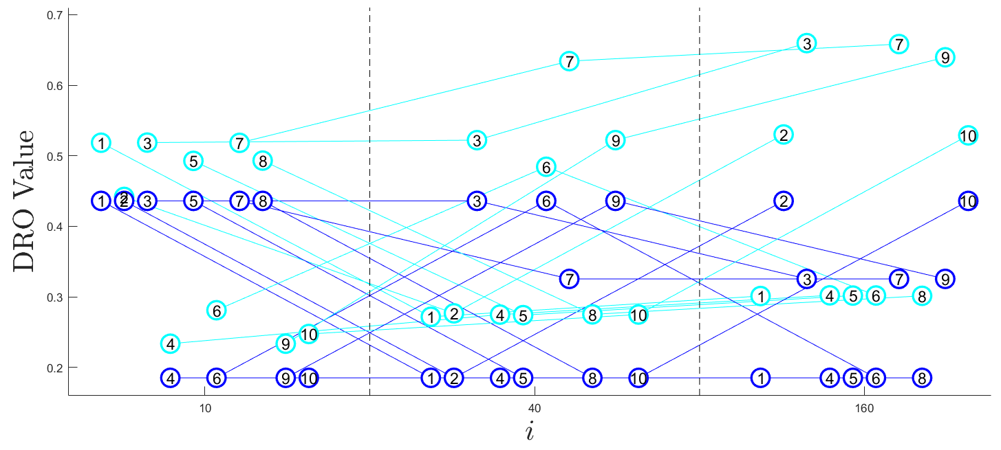
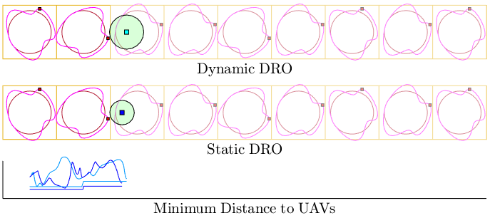
Figure 6 shows snapshots from the blue UAV traversing the area monitored by the 151 to 159th red UAVs in one of the realizations. The radius of the circle moving with vehicle $B$ represents the root of the minimum squared distance from the red UAVs as obtained from the solution of the DRO. The dynamic DRO circle is larger than the static one since a better optimum is obtained in this case due to the ambiguity set being considerably smaller.

Figure 6: The figure depicts three snapshots of the blue UAV at (a) $T_{i}=151.6\cdot 2\pi$, (b) $T_{i}=154.4\cdot 2\pi$, and (c) $T_{i}=157.6\cdot 2\pi$. The upper and lower row of vehicle trajectories in each picture shows the outcome of the dynamic and static DRO, respectively. The circles’ radius is the square root of the DRO value, given also in the corresponding piecewise constant plots that are shown below. We additionally plotted the evolution of the minimum distance between the blue UAV and the red UAVs during the traversal, in cyan and blue, for the dynamic and the static DRO, respectively. The part of the snapshots with faded color includes the red UAVs that have not been observed by the blue one.

VII Conclusions

We have developed a framework to compute ambiguity sets of unknown probability distributions using data collected from dynamically varying processes that retain the same probabilistic guarantees as their static counterparts. Under exact knowledge of the dynamic evolution of the data and full-state measurements, we have identified conditions on its growth rate and the sampling rate that ensure the ambiguity sets shrink with time. In the presence of numerical errors and/or disturbances in the dynamics, we have also quantified the number of exploitable past samples necessary to establish the reduction of the ambiguity sets. We have generalized these results to the case of partial-state measurements of linear time-varying systems building on their sample-data observability properties. Future work will exploit the construction of time-varying ambiguity sets in receding horizon DRO problems and explore the extension of the results to consider data storage limitations, stochastic descriptions of the disturbances, measurement noise in the observations, and scenarios with incomplete knowledge of the dynamic evolution of the data.

Appendix A Appendix

Here we provide proofs of various results of the paper.

A-A Proofs from Section III

Proof:

Part (i) follows directly from the fact that $\{\xi_{0}^{i}\}_{i\in[N^{\flat}:\bar{N}]}$ are i.i.d. and $\Phi_{T}$ is measurable, implying that all $\xi_{T}^{i}=\Phi_{T}\circ\xi_{0}^{i}$ are also i.i.d. (see [19, Remark 2.15(iii)]). For part (ii), note that $\bar{P}_{\xi_{T}}^{N}=\frac{1}{N}\sum_{i=N^{\flat}}^{\bar{N}}\delta_{\bar{\xi}_{T}^{i}}=\frac{1}{N}\sum_{i=N^{\flat}}^{\bar{N}}\delta_{\Phi_{T,t_{i}}(\xi_{t_{i}}^{i})}=\frac{1}{N}\sum_{i=N^{\flat}}^{\bar{N}}\delta_{\xi_{T}^{i}}=\widehat{P}_{\xi_{T}}^{N}$, as desired, where we have exploited the fact that $\Phi_{T,t_{i}}(\xi_{t_{i}}^{i})=\Phi_{T,t_{i}}\circ\Phi_{t_{i}}(\xi_{0}^{i})=\Phi_{T}(\xi_{0}^{i})$ in the second to last equality. ∎

The proof of Proposition III.4 is based on the following comparison lemma.

Lemma A.1

(Polynomial growth). Consider a locally absolutely continuous function $\theta:\mathbb{R}_{\geq 0}\to\mathbb{R}_{\geq 0}$ which satisfies for almost all $t\geq 0$

$$\theta(t)>0\Rightarrow\dot{\theta}(t)\leq\alpha(t)\theta(t)+M_{1}\theta(t)^{q},$$ (35)

for certain $q\in(-\infty,1)$ and $M_{1}>0$, where the function $\alpha$ is locally integrable and satisfies (10) for certain $M_{2}>0$. Then,

$$\theta(t)\leq e^{M_{2}}(1+M_{1}(1-q)t)^{\frac{1}{1-q}}(1+\theta_{0}),$$ (36)

where $\theta_{0}=\theta(0)$.

Proof:

Let $A(t)=\int_{0}^{t}\alpha(s)ds$ and $\bar{A}(t):=\min_{0\leq s\leq t}A(s)$. Since $A(0)=0$, also $\bar{A}(0)=0$. Furthermore, $\bar{A}$ is locally absolutely continuous due to the fact that the same property holds for $A$. From the latter, combined with the fact that $\bar{A}$ is nonincreasing and satisfies $\bar{A}(0)=0$, it follows that there exists a nonnegative locally integrable function $\bar{\alpha}$ with $\bar{A}(t)=-\int_{0}^{t}\bar{\alpha}(s)ds$, for all $t\geq 0$. Then, if we define $\widehat{\alpha}(t):=\alpha(t)+\bar{\alpha}(t)$, $t\geq 0$, we obtain for all $t\geq 0$,

$$\widehat{\alpha}(t) \geq\alpha(t),$$ (37a)

$$\int_{0}^{t}\widehat{\alpha}(s)ds \geq 0,$$ (37b)

$$\int_{0}^{t}\widehat{\alpha}(s)ds \leq M_{2},$$ (37c)

Indeed, (37a) follows directly from the fact that $\bar{\alpha}$ is nonnegative. In addition, we have that $\int_{0}^{t}\widehat{\alpha}(s)ds=\int_{0}^{t}\alpha(s)ds+\int_{0}^{t}\bar{\alpha}(s)ds=A(t)-\bar{A}(t)=A(t)-\min_{0\leq s\leq t}A(s)\geq 0$, which establishes (37b). Finally, given that $\bar{A}(t)=\min_{0\leq s\leq t}A(s)=\int_{0}^{\tau}\alpha(s)ds$ for some $\tau\in[0,t]$, we get that $\int_{0}^{t}\widehat{\alpha}(s)ds=\int_{0}^{t}\alpha(s)ds-\bar{A}(t)=\int_{0}^{t}\alpha(s)ds-\int_{0}^{\tau}\alpha(s)ds=\int_{\tau}^{t}\alpha(s)ds\leq M_{2}$, because of (10). From (35) and (37a), we obtain for almost all $t\geq 0$, $\theta(t)>0\Rightarrow\dot{\theta}(t)\leq\widehat{\alpha}(t)\theta(t)+M_{1}\theta(t)^{q}$. Hence, by defining

$$\sigma(t):=\theta(t/M_{1}),t\geq 0,$$ (38)

it follows that for almost all $t\geq 0$,

$$\sigma(t)>0\Rightarrow\dot{\sigma}(t)=\frac{1}{M_{1}}\dot{\theta}(t/M_{1})\leq\gamma(t)\sigma(t)+\sigma(t)^{q},$$ (39)

with $\gamma(t):=1/M_{1}\widehat{\alpha}(t/M_{1})$. Then, we get from (37b) that

$$\int_{0}^{t}\gamma(s)ds\geq 0,\quad\forall t\geq 0,$$ (40)

and from (37c) that

$$\int_{0}^{t}\gamma(s)ds=\int_{0}^{t}\frac{1}{M_{1}}\widehat{\alpha}\Big{(}\frac{s}{M_{1}}\Big{)}ds=\int_{0}^{t/M_{1}}\widehat{\alpha}(\tau)d\tau\leq M_{2},$$ (41)

for all $t\geq 0$. Now, let $\lambda$ be the solution of

$$\dot{\lambda}(t)=\gamma(t)\lambda(t)+\lambda(t)^{q},\quad\lambda(0)=\sigma(0)+1,$$ (42)

which is defined for all $t\geq 0$ and is nondecreasing. We claim

$$\lambda(t)\geq\sigma(t),\quad\textup{for all}\;t\geq 0.$$ (43)

Indeed, suppose on the contrary that $\sigma(T)>\lambda(T)$ for certain $T>0$. Define $\tau:=\inf\{\bar{t}\geq 0\,|\,\sigma(t)>\lambda(t),\forall t\in(\bar{t},T]\}$. Then,

$$\sigma(t) >\lambda(t),\;\forall t\in(\tau,T],$$ (44a)

$$\sigma(\tau) =\lambda(\tau).$$ (44b)

By (39), (42), (44b), and the comparison lemma [18, Lemma 3.4], we get that $\sigma(t)\leq\lambda(t)$ for all $t\in(\tau,T]$, contradicting (44a). We next show that the absolutely continuous function

$$\eta(t):=e^{\int_{0}^{t}\gamma(s)ds}(1+t(1-q))^{\frac{1}{1-q}}(1+\theta_{0}),t\geq 0,$$ (45)

satisfies

$$\dot{\eta}(t)\geq\gamma(t)\eta(t)+\eta(t)^{q}$$ (46)

for almost all $t\geq 0$. Indeed, note that $\dot{\eta}(t)=\gamma(t)\eta(t)+e^{\int_{0}^{t}\gamma(s)ds}(1+\theta_{0})(1+t(1-q))^{\frac{q}{1-q}}$ for almost all $t\geq 0$. Solving with respect to $1+t(1-q)$ in (45), we deduce

$$\dot{\eta}(t) =\gamma(t)\eta(t)+e^{\int_{0}^{t}\gamma(s)ds}(1+\theta_{0})\bigg{(}\frac{\eta(t)}{e^{\int_{0}^{t}\gamma(s)ds}(1+\theta_{0})}\bigg{)}^{q}$$

$$=\gamma(t)\eta(t)+\big{(}e^{\int_{0}^{t}\gamma(s)ds}(1+\theta_{0})\big{)}^{1-q}\eta(t)^{q},$$

which implies (46), due to (40) and the fact that $1-q>0$. Thus, since by (38) and (42) it holds that $\eta(0)=1+\theta(0)=1+\sigma(0)=\lambda(0)$, we get from (42), (46), and the comparison lemma [18, Lemma 3.4], that $\eta(t)\geq\lambda(t)$ for all $t\geq 0$. Hence, from (43) and the definition of $\sigma$, we have that $\eta(t)\geq\theta(\frac{t}{M_{1}})$ for all $t\geq 0$. From the latter, (41), and (45), we deduce (36), which completes the proof. ∎

We are ready to prove Proposition III.4.

Proof:

Consider an initial condition $\xi_{0}\in\mathbb{R}^{d}$ and let $\xi$ denote the solution of (1) defined for all $t\geq 0$. Then, $t\mapsto V(\xi(t))$ is differentiable, and from (8b),

$$V(\xi(t))>0\Rightarrow\frac{d}{dt}V(\xi(t)) =DV(\xi(t))F(t,\xi(t))$$

$$\leq\alpha(t)V(\xi(t))+M_{1}V(\xi(t))^{q}.$$

Then, if $M_{1}=0$, we obtain by the comparison lemma [18, Lemma 3.4] that $V(\xi(t))\leq V(\xi_{0})e^{\int_{0}^{t}\alpha(s)ds}$ for all $t\geq 0$, and thus, by (8a), that (9) holds. If $M_{1}>0$, then, by using Lemma A.1 with $\theta(t):=V(\xi(t))$, we have from (36) that $V(\xi(t))\leq e^{M_{2}}(1+M_{1}(1-q)t)^{\frac{1}{1-q}}(1+V(\xi_{0}))$ for all $t\geq 0$. Consequently, it follows from (8a) that

$$\|\xi(t)\|\leq(e^{M_{2}}(1+a_{2}\|\xi_{0}\|^{r})/a_{1})^{\frac{1}{r}}(1+M_{1}(1-q)t)^{\frac{1}{r(1-q)}}$$

for all $t\geq 0$, which establishes (11) with $\bar{M}$ and $\bar{c}$ as given by (12). The proof is complete. ∎

Proof:

It suffices to show that $\lim_{x\to 0}h^{-1}(ax)/x^{\frac{1}{\bar{q}}}=0$, or equivalently, that

$$h^{-1}(ax)^{\frac{\bar{q}+2}{2}}/(x^{\frac{1}{\bar{q}}})^{\frac{\bar{q}+2}{2}}\to 0.$$

Using L’Hôpital’s rule and $\bar{q}>2$, it follows that there exists $\bar{y}>0$ with $h(y)>y^{\frac{\bar{q}+2}{2}}$ for all $0<y\leq\bar{y}$. Thus,

$$h^{-1}(ax)^{\frac{\bar{q}+2}{2}}/(x^{\frac{1}{\bar{q}}})^{\frac{\bar{q}+2}{2}} <h(h^{-1}(ax))/(x^{\frac{1}{\bar{q}}})^{\frac{\bar{q}+2}{2}}$$

$$=ax/x^{\frac{\bar{q}+2}{2\bar{q}}}=ax^{\frac{\bar{q}-2}{2\bar{q}}}\to 0,$$

since $\bar{q}>2$, and we get the result. ∎

A-B Proofs from Section IV

The proof of Theorem IV.1 relies on the following elementary result on the Wasserstein distance between two discrete distributions with the same number of elements.

Lemma A.2

(Wasserstein distance of discrete distributions). Consider the finite sequences $(X_{i})_{i=1}^{N}$, $(Y_{i})_{i=1}^{N}$ in $\mathbb{R}^{d}$ and the corresponding discrete distributions $\widehat{\mu}_{X}^{N}=\frac{1}{N}\sum_{i=1}^{N}\delta_{X_{i}}$, $\widehat{\mu}_{Y}^{N}=\frac{1}{N}\sum_{i=1}^{N}\delta_{Y_{i}}$. Then, it holds that $W_{p}(\widehat{\mu}_{X}^{N},\widehat{\mu}_{Y}^{N})\leq(\frac{1}{N}\sum_{i=1}^{N}\|X_{i}-Y_{i}\|^{p})^{\frac{1}{p}}$.

Proof:

Consider the probability measure $\pi=\frac{1}{N}\sum_{i=1}^{N}\delta_{(X_{i},Y_{i})}$ on $\mathbb{R}^{d}\times\mathbb{R}^{d}$. Then, it follows that $\widehat{\mu}_{X}^{N}$, $\widehat{\mu}_{Y}^{N}$ are marginals of $\pi$ and that $W_{p}(\widehat{\mu}_{X}^{N},\widehat{\mu}_{Y}^{N})\leq(\int_{\mathbb{R}^{d}\times\mathbb{R}^{d}}\|x-y\|^{p}\pi(dx,dy))^{\frac{1}{p}}=(\frac{1}{N}\sum_{i=1}^{N}\|X_{i}-Y_{i}\|^{p})^{\frac{1}{p}}$, as claimed. ∎

Proof:

Notice that the true distribution $P_{\xi_{T}}$ of the system state at $T$ will be supported in the compact set $\Phi_{T}(K)$. Thus, we get from (14) and Corollary III.3 that for the given confidence $1-\beta$, the Wasserstein distance between the ideal empirical distribution $\widehat{P}_{\xi_{T}}^{N}$ in (3) and $P_{\xi_{T}}$ will satisfy $\mathbb{P}(W_{p}(\widehat{P}_{\xi_{T}}^{N},P_{\xi_{T}})\leq\varepsilon_{N}(\beta,\rho_{T}))\geq 1-\beta$. Based on the latter, to establish (18a), it suffices to show that

$$W_{p}(\bar{P}_{\xi_{T}}^{N},\widehat{P}_{\xi_{T}}^{N}) \leq\bar{\varepsilon}_{N}(\Delta),$$ (47)

and take into account (18b) and the triangle inequality for $W_{p}$.

To show (47), recall that $\widehat{P}_{\xi_{T}}^{N}=\frac{1}{N}\sum_{i=N^{\flat}}^{\bar{N}}\delta_{\xi_{T}^{i}}$ and that $\xi_{T}^{i}=\Phi_{T,t_{i}}(\xi_{t_{i}}^{i})$ for each $i$. Then, given that $t_{i+1}-t_{i}\leq\Delta$ for each $i$ and taking into account (17), and that $t_{\bar{N}}=T$, we get from Lemma A.2 that

$$W_{p}(\bar{P}_{\xi_{T}}^{N},\widehat{P}_{\xi_{T}}^{N})\leq\Big{(}\frac{1}{N}\sum_{i=N^{\flat}}^{\bar{N}}\|\xi_{T}^{i}-\bar{\xi}_{T}^{i}\|^{p}\Big{)}^{\frac{1}{p}}$$

$$=\Big{(}\frac{1}{N}\sum_{i=N^{\flat}}^{\bar{N}}\|\Phi_{T,t_{i}}(\xi_{t_{i}}^{i})-\Phi^{\textup{num}}_{T,t_{i}}(\xi_{t_{i}}^{i})\|^{p}\Big{)}^{\frac{1}{p}}$$

$$\leq\Big{(}\frac{1}{N}\sum_{i=N^{\flat}}^{\bar{N}}\mathfrak{K}^{p}(e^{L(T-t_{i})}-1)^{p}\Big{)}^{\frac{1}{p}}$$

$$\leq\mathfrak{K}\Big{(}\frac{1}{N}\sum_{i=1}^{N}(e^{L\Delta(N-i)}-1)^{p}\Big{)}^{\frac{1}{p}}=\mathfrak{K}\Big{(}\frac{1}{N}\sum_{i=1}^{N-1}(e^{L\Delta i}-1)^{p}\Big{)}^{\frac{1}{p}}.$$

Then, the result is a consequence of the derived bound and the fact that for any $a>0$, $p\geq 1$, and $N\in\mathbb{N}$, it holds that $\sum_{i=1}^{N-1}(e^{ai}-1)^{p}\leq\int_{1}^{N}(e^{as}-1)^{p}ds$. ∎

A-C Proofs from Section V

Proof:

Under H1 in Assumption V.1,

$$\bm{\mathcal{O}}_{i}e^{A(t_{i}^{\ell}-t_{i}^{1})}=\bm{\mathcal{O}}_{\ell}(e^{A\Delta^{\prime}},C):=\left(\begin{matrix}C\\ Ce^{A\Delta^{\prime}}\\ \vdots\\ C\big{(}e^{A\Delta^{\prime}}\big{)}^{\ell-1}\end{matrix}\right).$$ (48)

In addition, due to H1, it follows that system (19) is $\Delta^{\prime}$-sampled observable [28, Proposition 6.2.11], namely, the pair $(e^{A\Delta^{\prime}},C)$ is observable. Thus, the observability matrix $\bm{\mathcal{O}}_{d}(e^{A\Delta^{\prime}},C)$ corresponding to this pair has full rank $d$. Since $\ell\geq d$, $\bm{\mathcal{O}}_{\ell}(e^{A\Delta^{\prime}},C)$ is also of full rank $d$, which by (48), establishes left invertibility of $\bm{\mathcal{O}}_{i}$. When H2 holds, the result follows analogously from the Corollary in Section IV of [20], which implies that

$${\rm rank}(\bm{\mathcal{O}}_{i})\equiv{\rm rank}\Big{(}\bm{\mathcal{O}}_{t_{i}^{1}\cdots t_{i}^{(\bar{d}+1)d}}^{\exp-}\Big{)}=d.$$

Thus, since $\ell\geq(\bar{d}+1)d$, we also obtain that $\bm{\mathcal{O}}_{i}$ is of full rank, and hence, left invertible. Finally, the same approach can be followed under H3, with left invertibility of $\bm{\mathcal{O}}_{i}$ guaranteed by [32, Theorem 2]. ∎

Before proceeding with the proof of Proposition V.4, we state some intermediate results to ensure robust invertibility of the sample-observability matrix $\bm{\mathcal{O}}_{i}$. Given $i\in[1:\bar{N}]$, let

$${\mathcal{W}_{\tau(i)}(t_{i}^{1})\big{|}_{[t_{i}^{l},t_{i}^{l+1}]}} :=\int_{t_{i}^{l}}^{t_{i}^{l}+\tau_{l}(i)}K(s,t_{i}^{1}+\tau(i))ds,$$ (49)

for each $l\in[1:\ell-1]$, with the intra-trajectory inter-sampling-time lengths $\tau_{l}(i)=t_{i}^{l+1}-t_{i}^{l}$ as in (24), and $\tau(i)=t_{i}^{\ell}-t_{i}^{1}$. Also, recall that $K_{s}(s,t)=\frac{\partial}{\partial s}K(s,t)$, which is continuous because of the regularity hypotheses of Assumption V.3.

Lemma A.3

(Integral-limits inequalities). For each $l\in[1:\ell-1]$, the integral ${\mathcal{W}_{\tau(i)}(t_{i}^{1})\big{|}_{[t_{i}^{l},t_{i}^{l+1}]}}$ satisfies

$$\Big{\|}\mathcal{W}_{\tau(i)}(t_{i}^{1})\big{|}_{[t_{i}^{l},t_{i}^{l+1}]}-\frac{\tau_{l}(i)}{2}( K(t_{i}^{l},t_{i}^{1}+\tau(i))$$

$$+K(t_{i}^{l+1},t_{i}^{1}+\tau(i)))\Big{\|}$$

$$\leq \frac{\tau_{l}^{2}(i)}{4}\max_{s\in[t_{i}^{l},t_{i}^{l+1}]}\|K_{s}(s,t_{i}^{1}+\tau(i))\|.$$

Proof:

From the mean value inequality,

$$\Big{\|}\mathcal{W}_{\tau(i)}(t_{i}^{1})\big{|}_{[t_{i}^{l},t_{i}^{l+1}]}-\frac{\tau_{l}(i)}{2}(K(t_{i}^{l},t_{i}^{1}+\tau(i))$$

$$\hskip 112.00014pt+K(t_{i}^{l+1},t_{i}^{1}+\tau(i)))\Big{\|}$$

$$=\bigg{\|}\int_{t_{i}^{l}}^{t_{i}^{l}+\frac{\tau_{l}(i)}{2}}(K(s,t_{i}^{1}+\tau(i))-K(t_{i}^{l},t_{i}^{1}+\tau(i)))ds$$

$$\quad+\int_{t_{i}^{l}+\frac{\tau_{l}(i)}{2}}^{t_{i}^{l}+\tau_{l}(i)}(K(s,t_{i}^{1}+\tau(i))-K(t_{i}^{l+1},t_{i}^{1}+\tau(i)))ds\bigg{\|}$$

$$\leq\int_{t_{i}^{l}}^{t_{i}^{l}+\frac{\tau_{l}(i)}{2}}(s-t_{i}^{l})ds\max_{s\in[t_{i}^{l},t_{i}^{l}+\frac{\tau_{l}(i)}{2}]}\|K_{s}(s,t_{i}^{1}+\tau(i))\|$$

$$\quad+\int_{t_{i}^{l}+\frac{\tau_{l}(i)}{2}}^{t_{i}^{l}+\tau_{l}(i)}\Big{(}s-t_{i}^{l}-\frac{\tau_{l}(i)}{2}\Big{)}ds$$

$$\hskip 82.00009pt\times\max_{s\in[t_{i}^{l}+\frac{\tau_{l}(i)}{2},t_{i}^{l+1}]}\|K_{s}(s,t_{i}^{1}+\tau(i))\|$$

$$\leq\frac{\tau_{l}^{2}(i)}{4}\max_{s\in[t_{i}^{l},t_{i}^{l+1}]}\|K_{s}(s,t_{i}^{1}+\tau(i))\|,$$

establishing the result. ∎

The following result provides an upper bound for the distance between the matrices $\bm{\mathcal{O}}_{i}^{\top}\bm{W}_{i}\bm{W}_{i}\bm{\mathcal{O}}_{i}$ and $\mathcal{W}_{\tau(i)}(t_{i}^{1})$ in the induced Euclidean norm.

Lemma A.4

(Distance between $\bm{\mathcal{O}}_{i}^{\top}\bm{W}_{i}\bm{W}_{i}\bm{\mathcal{O}}_{i}$ and $\mathcal{W}_{\tau(i)}(t_{i}^{1})$). Let $\mathcal{W}_{\tau(i)}(t_{i}^{1})$ and $\bm{W}_{i}$ as given by (22) and (25), and consider the sample-observability matrix $\bm{\mathcal{O}}_{i}$ in (20) and an intra-trajectory inter-sampling-time bound $\Delta^{\prime}>0$. Then,

$$\|\bm{\mathcal{O}}_{i}^{\top}\bm{W}_{i}\bm{W}_{i}\bm{\mathcal{O}}_{i} -\mathcal{W}_{\tau(i)}(t_{i}^{1})\|$$

$$\leq \frac{\tau(i)\Delta^{\prime}}{4}\max_{s\in[t_{i}^{1},t_{i}^{1}+\tau(i)]}\|K_{s}(s,t_{i}^{1}+\tau(i))\|.$$ (50)

Proof:

From the definitions of $\bm{\mathcal{O}}_{i}$ in (20), $K(s,t)$ in (21), $\mathcal{W}_{\tau(i)}(t_{i}^{1})$ in (22), the $\tau_{l}(i)$’s in (24), the matrix $\bm{W}_{i}$ in (25), and the matrices $\mathcal{W}_{\tau(i)}(t_{i}^{1})\big{|}_{[t_{i}^{l},t_{i}^{l+1}]}$ in (49), we have

$$\|\bm{\mathcal{O}}_{i}^{\top}\bm{W}_{i}\bm{W}_{i}\bm{\mathcal{O}}_{i}-\mathcal{W}_{\tau(i)}(t_{i}^{1})\|$$

$$=\|\left(\begin{matrix}w_{1}(i)\Phi(t_{i}^{1},t_{i}^{\ell})^{\top}C(t_{i}^{1})^{\top}&\cdots&w_{\ell}(i)\Phi(t_{i}^{\ell},t_{i}^{\ell})^{\top}C(t_{i}^{\ell})^{\top}\end{matrix}\right)$$

$$\hskip 85.00012pt\left.\times\left(\begin{matrix}w_{1}(i)C(t_{i}^{1})\Phi(t_{i}^{1},t_{i}^{\ell})\\ \vdots\\ w_{\ell}(i)C(t_{i}^{\ell})\Phi(t_{i}^{\ell},t_{i}^{\ell})\end{matrix}\right)-\mathcal{W}_{\tau(i)}(t_{i}^{1})\right\|$$

$$=\bigg{\|}\sum_{l=1}^{\ell}w_{l}^{2}(i)K(t_{i}^{l},t_{i}^{1}+\tau(i))-\mathcal{W}_{\tau(i)}(t_{i}^{1})\bigg{\|}$$

$$=\bigg{\|}\sum_{l=1}^{\ell-1}\frac{\tau_{l}(i)}{2}(K(t_{i}^{l},t_{i}^{1}+\tau(i))+K(t_{i}^{l+1},t_{i}^{1}+\tau(i)))$$

$$\hskip 180.00027pt-\mathcal{W}_{\tau(i)}(t_{i}^{1})\bigg{\|}$$

$$\leq\sum_{l=1}^{\ell-1}\Big{\|}\frac{\tau_{l}(i)}{2}(K(t_{i}^{l},t_{i}^{1}+\tau(i))+K(t_{i}^{l+1},t_{i}^{1}+\tau(i)))$$

$$\hskip 160.00024pt-\mathcal{W}_{\tau(i)}(t_{i}^{1})\big{|}_{[t_{i}^{l},t_{i}^{l+1}]}\Big{\|}$$

$$\leq\sum_{l=1}^{\ell-1}\frac{\tau_{l}^{2}(i)}{4}\max_{s\in[t_{i}^{l},t_{i}^{l+1}]}\|K_{s}(s,t_{i}^{1}+\tau(i))\|,$$ (51)

where we have used Lemma A.3 in the last inequality. Thus, from the bound on the maximum inter-sampling time, we get (A.4), which establishes the result. ∎

When the system is time invariant, i.e., $A(t)\equiv A$ and $C(t)\equiv C$, we obtain the following corollary to Lemma A.4, with a more explicit bound for $\|\bm{\mathcal{O}}_{i}^{\top}\bm{W}_{i}\bm{W}_{i}\bm{\mathcal{O}}_{i}-\mathcal{W}_{\tau(i)}(t_{i}^{1})\|$.

Corollary A.5

(Distance between $\bm{\mathcal{O}}_{i}^{\top}\bm{W}_{i}\bm{W}_{i}\bm{\mathcal{O}}_{i}$ and $\mathcal{W}_{\tau(i)}(t_{i}^{1})$ for LTI systems). Under the assumptions of Lemma A.4, when (19) is time invariant,

$$\|\bm{\mathcal{O}}_{i}^{\top}\bm{W}_{i}\bm{W}_{i}\bm{\mathcal{O}}_{i}- \mathcal{W}_{\tau(i)}(t_{i}^{1})\|$$

$$\leq\frac{\tau(i)\Delta^{\prime}}{2}\max_{s\in[0,\tau(i)]}\|\widehat{K}(s-\tau(i))A\|.$$

Proof:

From (28), note that $\dot{\widehat{K}}(s)=\frac{d}{ds}(e^{A^{\top}s}C^{\top}Ce^{As})=A^{\top}e^{A^{\top}s}C^{\top}Ce^{As}+e^{A^{\top}s}C^{\top}Ce^{As}A$. Since the spectral norm of a matrix equals that of its transpose, it follows that $\|\dot{\widehat{K}}(s)\|\leq 2\|\widehat{K}(s)A\|$. Combining this with the bound for $\|\bm{\mathcal{O}}_{i}^{\top}\bm{W}_{i}\bm{W}_{i}\bm{\mathcal{O}}_{i}-\mathcal{W}_{\tau(i)}(t_{i}^{1})\|$ in Lemma A.4, and the fact that $K(s,t)=\widehat{K}(s-t)$,

$$\frac{\tau(i)\Delta^{\prime}}{4}\max_{s\in[t_{i}^{1},t_{i}^{1}+\tau(i)]}\|K_{s}(s,t_{i}^{1}+\tau(i))\|$$

$$=\frac{\tau(i)\Delta^{\prime}}{4}\max_{s\in[t_{i}^{1},t_{i}^{1}+\tau(i)]}\|\dot{\widehat{K}}(s-(t_{i}^{1}+\tau(i)))\|$$

$$=\frac{\tau(i)\Delta^{\prime}}{4}\max_{s\in[0,\tau(i)]}\|\dot{\widehat{K}}(s-\tau(i))\|$$

$$\leq\frac{\tau(i)\Delta^{\prime}}{2}\max_{s\in[0,\tau(i)]}\|\widehat{K}(s-\tau(i))A\|,$$

which completes the proof. ∎

Based on the obtained results, we prove Proposition V.4.

Proof:

Let $i\in[1:\bar{N}]$ and note that for any pair of symmetric matrices $P$ and $Q$,

$$\lambda_{\min}(P) =\min_{\|x\|=1}x^{\top}Px=\min_{\|x\|=1}x^{\top}(Q+P-Q)x$$

$$\leq\min_{\|x\|=1}x^{\top}Qx+\max_{\|x\|=1}x^{\top}(P-Q)x$$

$$=\lambda_{\min}(Q)+\|P-Q\|.$$

Combining this observation with the result of Lemma A.4,

$$\lambda_{\min}(\mathcal{W}_{\tau(i)}(t_{i}^{1}))\leq \;\lambda_{\min}(\bm{\mathcal{O}}_{i}^{\top}\bm{W}_{i}\bm{W}_{i}\bm{\mathcal{O}}_{i})$$

$$+\|\bm{\mathcal{O}}_{i}^{\top}\bm{W}_{i}\bm{W}_{i}\bm{\mathcal{O}}_{i}-\mathcal{W}_{\tau(i)}(t_{i}^{1})\|$$

$$\leq \;\lambda_{\min}(\bm{\mathcal{O}}_{i}^{\top}\bm{W}_{i}\bm{W}_{i}\bm{\mathcal{O}}_{i})$$

$$+\frac{\tau(i)\Delta^{\prime}}{4}\max_{s\in[t_{i}^{1},t_{i}^{1}+\tau(i)]}\|K_{s}(s,t_{i}^{1}+\tau(i))\|.$$

Thus, we get from (23) and by plugging in (26) that

$$\lambda_{\min}(\bm{\mathcal{O}}_{i}^{\top}\bm{W}_{i}\bm{W}_{i}\bm{\mathcal{O}}_{i})$$

$$\geq\lambda_{\min}(\mathcal{W}_{\tau(i)}(t_{i}^{1}))-\frac{\tau(i)\Delta^{\prime}}{4}\max_{s\in[t_{i}^{1},t_{i}^{1}+\tau(i)]}\|K_{s}(s,t_{i}^{1}+\tau(i))\|$$

$$\geq\lambda_{\min}(\mathcal{W}_{\tau(i)}(t_{i}^{1}))-\frac{\tau(i)(1-a)\lambda_{\min}\big{(}\mathcal{W}_{\tau^{\textup{low}}}(t)|_{0}^{T-\tau^{\textup{low}}}\big{)}}{\tau^{\textup{up}}}$$

$$\hskip 75.0001pt\times\frac{\max_{s\in[t_{i}^{1},t_{i}^{1}+\tau(i)]}\|K_{s}(s,t_{i}^{1}+\tau(i))\|}{\max_{\tau^{\textup{low}}\leq t\leq T,\max\{0,t-\tau^{\textup{up}}\}\leq s\leq t}\|K_{s}(s,t)\|}$$

$$\geq\lambda_{\min}(\mathcal{W}_{\tau(i)}(t_{i}^{1}))-\frac{\tau(i)}{\tau^{\textup{up}}}(1-a)\lambda_{\min}\big{(}\mathcal{W}_{\tau^{\textup{low}}}(t)|_{0}^{T-\tau^{\textup{low}}}\big{)}$$

$$\geq\lambda_{\min}(\mathcal{W}_{\tau(i)}(t_{i}^{1}))-(1-a)\lambda_{\min}\big{(}\mathcal{W}_{\tau^{\textup{low}}}(t)|_{0}^{T-\tau^{\textup{low}}}\big{)}$$

$$\hskip 110.00017pt\geq a\lambda_{\min}\big{(}\mathcal{W}_{\tau^{\textup{low}}}(t)|_{0}^{T-\tau^{\textup{low}}}\big{)},$$

which concludes the proof. ∎

The result of Corollary V.5 is obtained by the same arguments by using the bound from Corollary A.5 instead of that given in Lemma A.4. We are now in position to prove Proposition V.9.

Proof:

To show the result, note that $\bm{\zeta}^{i}=\bm{\mathcal{O}}_{i}\xi_{t_{i+\ell}}^{i}$, or equivalently, $\bm{W}_{i}\bm{\zeta}^{i}=\bm{W}_{i}\bm{\mathcal{O}}_{i}\xi_{t_{i+\ell}}^{i}$, and consequently $\xi_{t_{i+\ell}}^{i}=(\bm{W}_{i}\bm{\mathcal{O}}_{i})^{\dagger}\bm{W}_{i}\bm{\zeta}^{i}$, since $\bm{W}_{i}\bm{\mathcal{O}}_{i}$ is of full rank. Thus, we obtain

$$\|\widehat{\xi}_{t_{i+\ell}}^{i} -\xi_{t_{i+\ell}}^{i}\|=\|{(\bm{W}_{i}\bm{\mathcal{O}}_{i})^{\dagger}\bm{W}_{i}}(\widehat{\bm{\zeta}}^{i}-\bm{\zeta}^{i})\|$$

$$=\|(\bm{W}_{i}\bm{\mathcal{O}}_{i})^{\dagger}\bm{W}_{i}\bm{\delta}^{i}\|\leq\|(\bm{W}_{i}\bm{\mathcal{O}}_{i})^{\dagger}\|\|\bm{W}_{i}\bm{\delta}^{i}\|.$$ (52)

We upper bound the first term on the right hand side of the above inequality as

$$\|\bm{W}_{i}\bm{\delta}^{i}\| =\Big{(}\sum_{l=1}^{\ell}w_{l}^{2}(i)\|\delta_{l}^{i}\|^{2}\Big{)}^{\frac{1}{2}}$$

$$\leq\delta^{*}\Big{(}\frac{\tau_{1}(i)}{2}+\sum_{l=2}^{\ell-1}\frac{\tau_{l-1}(i)+\tau_{l}(i)}{2}+\frac{\tau_{\ell-1}(i)}{2}\Big{)}^{\frac{1}{2}}$$

$$=\delta^{*}\sqrt{\tau(i)}\leq\delta^{*}\sqrt{\tau^{\textup{up}}},$$

where we have use the definition of $w_{l}(i)$ from (25) and the bound $\delta^{*}$ on each $\delta_{l}^{i}$. While the second term satisfies

$$\|(\bm{W}_{i}\bm{\mathcal{O}}_{i})^{\dagger}\|=\sigma_{\max}((\bm{W}_{i}\bm{\mathcal{O}}_{i})^{\dagger})=\frac{1}{\sigma_{\min}(\bm{W}_{i}\bm{\mathcal{O}}_{i})},$$

with $\sigma_{\max}$ and $\sigma_{\min}$ denoting the largest and smallest nonzero singular value of the corresponding non-degenerate matrix, respectively. The second equality follows from the fact that $\bm{W}_{i}\bm{\mathcal{O}}_{i}$ is of full rank (see [21, Page 435, Proposition 4]). Thus, by taking into account (27) and that $\lambda_{\min}(\bm{\mathcal{O}}_{i}^{\top}\bm{W}_{i}\bm{W}_{i}\bm{\mathcal{O}}_{i})=\sigma_{\min}(\bm{W}_{i}\bm{\mathcal{O}}_{i})^{2}$, it follows from (52) that (32) is fulfilled. ∎

Finally, we give the proof of Theorem V.10.

Proof:

The proof is analogous to that of Theorem IV.1, with the key modification being establishment of (47) with $\bar{\varepsilon}_{N}$ as in (33). By taking into account (17), (32), the elementary inequality $(a+b)^{p}\leq 2^{p-1}(a^{p}+b^{p})$, which holds for any $a,b\geq 0$ and $p\geq 1$ [4, Lemma 2.4.6], and that the flow $\Phi$ is linear, as in the proof of Theorem IV.1, we obtain

$$W_{p}(\bar{P}_{\xi_{T}}^{N},\widehat{P}_{\xi_{T}}^{N})\leq\Big{(}\frac{1}{N}\sum_{i=N^{\flat}}^{\bar{N}}\|\xi_{T}^{i}-\bar{\xi}_{T}^{i}\|^{p}\Big{)}^{\frac{1}{p}}$$

$$=\Big{(}\frac{1}{N}\sum_{i=N^{\flat}}^{\bar{N}}\|\Phi_{T,t_{i}^{\ell}}(\xi_{t_{i}^{\ell}}^{i})-\Phi^{\textup{num}}_{T,t_{i}^{\ell}}(\widehat{\xi}_{t_{i}^{\ell}}^{i})\|^{p}\Big{)}^{\frac{1}{p}}$$

$$\leq\Big{(}\frac{2^{p-1}}{N}\sum_{i=N^{\flat}}^{\bar{N}}\big{(}\|\Phi_{T,t_{i}^{\ell}}(\xi_{t_{i}^{\ell}}^{i}-\widehat{\xi}_{t_{i}^{\ell}}^{i})\|^{p}$$

$$\hskip 70.0001pt+\|\Phi_{T,t_{i}^{\ell}}(\widehat{\xi}_{t_{i}^{\ell}}^{i})-\Phi^{\textup{num}}_{T,t_{i}^{\ell}}(\widehat{\xi}_{t_{i}^{\ell}}^{i})\|^{p}\big{)}\Big{)}^{\frac{1}{p}}$$

$$\leq\Big{(}\frac{2^{p-1}}{N}\sum_{i=N^{\flat}}^{\bar{N}}\big{(}(\varepsilon^{*})^{p}e^{pL(T-t_{i}^{\ell})}+\mathfrak{K}^{p}(e^{L(T-t_{i}^{\ell})}-1)^{p}\big{)}\Big{)}^{\frac{1}{p}}$$

$$\leq\Big{(}\frac{2^{p-1}}{N}\sum_{i=1}^{N}\big{(}(\varepsilon^{*})^{p}e^{pL\Delta(N-i)}+\mathfrak{K}^{p}(e^{L\Delta(N-i)}-1)^{p}\big{)}\Big{)}^{\frac{1}{p}}$$

$$=\Big{(}\frac{2^{p-1}}{N}\Big{[}(\varepsilon^{*})^{p}\sum_{i=0}^{N-1}e^{pL\Delta i}+\mathfrak{K}^{p}\sum_{i=1}^{N-1}(e^{L\Delta i}-1)^{p}\Big{]}\Big{)}^{\frac{1}{p}}$$

$$\leq\Big{(}\frac{2^{p-1}}{N}\Big{[}(\varepsilon^{*})^{p}\int_{0}^{N}e^{pL\Delta s}ds+\mathfrak{K}^{p}\int_{1}^{N}(e^{L\Delta s}-1)^{p}ds\Big{]}\Big{)}^{\frac{1}{p}}.$$

By evaluating the first integral in the latter expression we obtain the desired result. ∎

Dimitris Boskos Dimitris Boskos was born in Athens, Greece in 1981. He has received the Diploma in Mechanical Engineering from the National Technical University of Athens (NTUA), Greece, in 2005, the M.Sc. in Applied mathematics from the NTUA in 2008 and the Ph.D. in Applied mathematics from the NTUA in 2014. Between August 2014 and August 2018, he has been a Postdoctoral Researcher at the Department of Automatic Control, School of Electrical Engineering, Royal Institute of Technology (KTH), Stockholm, Sweden. Since August 2018, he is a Postdoctoral Researcher at the Department of Mechanical and Aerospace Engineering, University of California, San Diego, CA, USA. His research interests include distributionally robust optimization, distributed control of multi-agent systems, formal verification, and nonlinear observer design.

Jorge Cortés (M’02, SM’06, F’14) received the Licenciatura degree in mathematics from Universidad de Zaragoza, Zaragoza, Spain, in 1997, and the Ph.D. degree in engineering mathematics from Universidad Carlos III de Madrid, Madrid, Spain, in 2001. He held postdoctoral positions with the University of Twente, Twente, The Netherlands, and the University of Illinois at Urbana-Champaign, Urbana, IL, USA. He was an Assistant Professor with the Department of Applied Mathematics and Statistics, University of California, Santa Cruz, CA, USA, from 2004 to 2007. He is currently a Professor in the Department of Mechanical and Aerospace Engineering, University of California, San Diego, CA, USA. He is the author of Geometric, Control and Numerical Aspects of Nonholonomic Systems (Springer-Verlag, 2002) and co-author (together with F. Bullo and S. Martínez) of Distributed Control of Robotic Networks (Princeton University Press, 2009). At the IEEE Control Systems Society, he has been a Distinguished Lecturer (2010-2014), and is currently its Director of Operations and an elected member (2018-2020) of its Board of Governors. His current research interests include distributed control and optimization, network science, resource-aware control, nonsmooth analysis, reasoning and decision making under uncertainty, network neuroscience, and multi-agent coordination in robotic, power, and transportation networks.

Sonia Martínez (M’02-SM’07-F’18) is a Professor of Mechanical and Aerospace Engineering at the University of California, San Diego, CA, USA. She received the Ph.D. degree in Engineering Mathematics from the Universidad Carlos III de Madrid, Spain, in May 2002. Following a year as a Visiting Assistant Professor of Applied Mathematics at the Technical University of Catalonia, Spain, she obtained a Postdoctoral Fulbright Fellowship and held appointments at the Coordinated Science Laboratory of the University of Illinois, Urbana-Champaign during 2004, and at the Center for Control, Dynamical systems and Computation (CCDC) of the University of California, Santa Barbara during 2005. In a broad sense, her main research interests include the control of network systems, multi-agent systems, nonlinear control theory, and robotics. For her work on the control of underactuated mechanical systems she received the Best Student Paper award at the 2002 IEEE Conference on Decision and Control. She was the recipient of a NSF CAREER Award in 2007. For the paper “Motion coordination with Distributed Information,” co-authored with Jorge Cortés and Francesco Bullo, she received the 2008 Control Systems Magazine Outstanding Paper Award. She has served on the editorial board of the European Journal of Control (2011-2013) and the Journal of Geometric Mechanics (2009-present), and currently serves as a Senior Editor of the IEEE Transactions on Control of Network Systems.

References

- [1] S. Ammar, H. Feki, and J.-C. Vivalda, “Observability under sampling for bilinear system,” International Journal of Control, vol. 87, no. 2, p. 312–319, 2014.
- [2] S. Ammar, M. Massaoud, and J.-C. Vivalda, “Genericity of the strong observability for sampled systems,” SIAM Journal on Control and Optimization, vol. 56, no. 2, p. 1463–1490, 2018.
- [3] S. Ammar and J.-C. Vivalda, “On the preservation of observability under sampling,” Systems and Control Letters, vol. 52, no. 1, p. 7–15, 2004.
- [4] R. B. Ash, Real Analysis and Probability. Academic Press, 1972.
- [5] A. Ben-Tal, L. E. Ghaoui, and A. Nemirovski, Robust optimization. Princeton University Press, 2009.
- [6] A. Ben-Tal, D. D. Hertog, A. D. Waegenaere, B. Melenberg, and G. Rennen, “Robust solutions of optimization problems affected by uncertain probabilities,” Management Science, vol. 59, no. 2, p. 341–357, 2013.
- [7] D. Bertsimas, M. Sim, and M. Zhang, “Adaptive distributionally robust optimization,” Management Science, vol. 65, no. 2, p. 604–618, 2018.
- [8] J. Blanchet, Y. Kang, and K. Murthy, “Robust Wasserstein profile inference and applications to Machine Learning,” arXiv preprint arXiv:1610.05627, 2016.
- [9] J. Blanchet and K. Murthy, “Quantifying distributional model risk via optimal transport,” Mathematics of Operations Research, vol. 44, no. 2, pp. 565–600, 2019.
- [10] D. Boskos, J. Cortés, and S. Martínez, “Dynamic evolution of distributional ambiguity sets and precision tradeoffs in data assimilation,” in European Control Conference, Naples, Italy, 2019, pp. 2252–2257.
- [11] A. Cherukuri and J. Cortés, “Cooperative data-driven distributionally robust optimization,” IEEE Transactions on Automatic Control, 2018, submitted.
- [12] S. Dereich, M. Scheutzow, and R. Schottstedt, “Constructive quantization: Approximation by empirical measures,” Annales de l’Institut Henri Poincaré, Probabilités et Statistiques, vol. 49, no. 4, p. 1183–1203, 2013.
- [13] P. M. Esfahani and D. Kuhn, “Data-driven distributionally robust optimization using the Wasserstein metric: performance guarantees and tractable reformulations,” Mathematical Programming, no. 1-2, p. 115–166, 2018.
- [14] N. Fournier and A. Guillin, “On the rate of convergence in Wasserstein distance of the empirical measure,” Probability Theory and Related Fields, vol. 162, no. 3-4, p. 707–738, 2015.
- [15] R. Gao and A. Kleywegt, “Distributionally robust stochastic optimization with Wasserstein distance,” arXiv preprint arXiv:1604.02199, 2016.
- [16] R. Jiang and Y. Guan, “Data-driven chance constrained stochastic program,” Mathematical Programming, vol. 158, no. 1-2, p. 291–327, 2016.
- [17] I. Karafyllis and C. Kravaris, “From continuous-time design to sampled-data design of observers,” IEEE Transactions on Automatic Control, vol. 54, no. 9, p. 2169–2174, 2009.
- [18] H. Khalil, Nonlinear Systems. Prentice Hall, 2002.
- [19] A. Klenke, Probability theory: a comprehensive course. Springer, 2013.
- [20] G. Kreisselmeier, “On sampling without loss of observability/controllability,” IEEE Transactions on Automatic Control, vol. 44, no. 5, p. 1021–1025, 1999.
- [21] P. Lancaster and M. Tismenetsky, The theory of matrices: with applications. Elsevier, 1985.
- [22] B. C. Levy and R. Nikoukhah, “Robust state space filtering under incremental model perturbations subject to a relative entropy tolerance,” IEEE Transactions on Automatic Control, vol. 58, no. 3, p. 682–695, 2013.
- [23] D. Li and S. Martínez, “Online data assimilation in distributionally robust optimization,” arXiv preprint arXiv:180307984, 2018.
- [24] S. T. Rachev, L. Klebanov, S. V. Stoyanov, and F. Fabozzi, The methods of distances in the theory of probability and statistics. Springer, 2013.
- [25] S. Shafieezadeh-Abadeh, V. A. Nguyen, D. Kuhn, and P. M. Esfahani, “Wasserstein distributionally robust Kalman filtering,” in Advances in Neural Information Processing Systems, 2018, pp. 8474–8483.
- [26] A. Shapiro, “Distributionally robust stochastic programming,” SIAM Journal on Optimization, vol. 27, no. 4, p. 2258–2275, 2017.
- [27] A. Shapiro, D. Dentcheva, and A. Ruszczyński, Lectures on Stochastic Programming: Modeling and Theory. Philadelphia, PA: SIAM, 2014, vol. 16.
- [28] E. D. Sontag, Mathematical control theory: deterministic finite dimensional systems. Springer, 1998.
- [29] A. Stuart and A. R. Humphries, Dynamical systems and numerical analysis. Cambridge University Press, 1998, vol. 2.
- [30] C. Villani, Topics in optimal transportation. American Mathematical Society, 2003, no. 58.
- [31] L. Y. Wang, C. Li, G. Yin, L. Guo, and C.-Z. Xu, “State observability and observers of linear-time-invariant systems under irregular sampling and sensor limitations,” IEEE Transactions on Automatic Control, vol. 56, no. 11, p. 2639–2654, 2011.
- [32] S. Zeng and F. Allgöwer, “A general sampled observability result and its applications,” in IEEE Int. Conf. on Decision and Control, 2016, p. 3997–4002.
- [33] S. Zeng, H. Ishii, and F. Allgöwer, “Sampled observability and state estimation of linear discrete ensembles,” IEEE Transactions on Automatic Control, vol. 62, no. 5, p. 2406–2418, 2017.
- [34] M. Zorzi, “Robust Kalman filtering under model perturbations,” IEEE Transactions on Automatic Control, vol. 62, no. 6, p. 2902–2907, 2017.
![[Uncaptioned image]](/html/1909.11194/assets/x5.jpg) |