The New Physics Reach of Null Tests with $D\to\pi\ell\ell$ and $D_{s}\to K\ell\ell$ Decays

Abstract

$|\Delta c|=|\Delta u|=1$ processes are unique probes of flavor physics in the up-sector within and beyond the Standard Model (SM). SM tests with rare semileptonic charm meson decays are based on an approximate CP–symmetry, a superior GIM–mechanism, angular distributions, lepton-universality and lepton flavor conservation. We analyze the complete set of null test observables in $D\to\pi\ell\ell^{(\prime)}$ and $D_{s}\to K\ell\ell^{(\prime)}$ decays, $\ell^{(\prime)}=e,\mu$, and find large room for new physics safely above the SM contribution. We identify signatures of supersymmetry, leptoquarks and anomaly-free $U(1)^{\prime}$–models with generation-dependent charges, for which we provide explicit examples. $Z^{\prime}$–effects in $c\to u\ell\ell^{(\prime)}$ transitions can be sizable if both left-handed and right-handed couplings to quarks are present.

I Introduction

New physics (NP) can be probed in rare semileptonic charm decays Burdman:2001tf ; Paul:2011ar ; deBoer:2015boa ; Fajfer:2015mia ; Fajfer:2012nr ; deBoer:2018buv ; Cappiello:2012vg . Null test observables, already key to ongoing and future precision programs in rare semileptonic $b$-decays Kou:2018nap ; Cerri:2018ypt , are indispensable when methods to achieve sufficient theoretical control on decay amplitudes are not available. This is exactly the case in charm decays, subject to notorious resonance pollution and poor convergence of the heavy quark expansion Feldmann:2017izn . Null tests are based on approximate symmetry limits, which follow from parametric or structural features of the Standard Model (SM) that do not have to be present in general models beyond the SM. Useful limits include the suppression of CP-violation, lepton-nonuniversality and lepton flavor violation (LFV), and an efficient Glashow-Iliopoulos-Maiani (GIM) mechanism in $|\Delta c|=|\Delta u|=1$ processes. Looking for a breakdown of such symmetries above the residual SM background is a useful strategy when there is a limit only, or even none, and large room for NP. Null test searches with rare charm decays provide hence a unique opportunity to test the SM now.

Here we study the complete catalog of null tests in $D\to\pi\ell\ell^{(\prime)}$ and $D_{s}\to K\ell\ell^{(\prime)}$ decays, $\ell^{(\prime)}=e,\mu$. We closely follow deBoer:2015boa and include experimental updates and recent lattice results for $D\to\pi$ form factors Lubicz:2017syv ; Lubicz:2018rfs . While the decays $D\to\pi^{+}\pi^{-}\mu^{+}\mu^{-}$ and $D\to K^{+}K^{-}\mu^{+}\mu^{-}$ have been observed at a level consistent with the SM Aaij:2017iyr ; deBoer:2018buv ; Cappiello:2012vg , for the branching ratios of $D\to\pi\ell^{+}\ell^{-}$ and $D_{s}\to K\ell^{+}\ell^{-}$ only upper limits exist Tanabashi:2018oca . Experimental study is suitable for high luminosity flavor facilities LHCb Bediaga:2012py , Belle II Aushev:2010bq and BESIII Asner:2008nq . We also discuss signatures in concrete BSM models, specifically leptoquarks, supersymmetry, and flavorful $Z^{\prime}$-models. We comment on the complementarity between charm and $K,B$-flavor probes.

The plan of the paper is as follows: In Sec. II we review the predictions in the SM, taking into account improved form factor computations. In Sec. III constraints on Wilson coefficients are obtained, and null test observables for $D\to\pi\ell\ell^{(\prime)}$ and $D_{s}\to K\ell\ell^{(\prime)}$ decays, $\ell^{(\prime)}=e,\mu$, are analyzed. Signatures of concrete BSM models in $c\to u\ell\ell^{(\prime)}$ transitions are worked out in Sec. IV. In Sec. V we conclude. In App. A we provide details on the $D\to\pi$ form factors. Constraints from $D^{0}-\overline{D}^{0}$ mixing are discussed in App. B. In App. C we give details on and explicit examples of anomaly-free $Z^{\prime}$–models with generation-dependent charges.

II Standard Model predictions

We discuss exclusive rare charm meson decays in the SM. In Sec. II.1 we review the SM contribution in an effective field theory framework at the charm mass scale. We discuss resonant contributions from intermediate mesons in Sec. II.2. In Sec. II.3 we present the $D\to\pi\ell^{+}\ell^{-}$ and $D_{s}\to K\ell^{+}\ell^{-}$ differential branching ratios and discuss SM uncertainties.

II.1 An effective field theory approach to charm physics

Rare $c\to u\ell^{+}\ell^{-}$ processes can be described by the effective Hamiltonian,

$$\mathcal{H}_{\rm eff}\supset-\frac{4G_{F}}{\sqrt{2}}\frac{\alpha_{e}}{4\pi}\biggl{[}\sum_{i=7,9,10,S,P}\bigl{(}C_{i}O_{i}+C_{i}^{\prime}O_{i}^{\prime}\bigr{)}+\sum_{i=T,T5}C_{i}O_{i}+\sum_{q=d,s}V_{cq}^{*}V_{uq}\sum_{i=1}^{2}C_{i}O_{i}^{q}\biggr{]}\,,$$ (1)

where the dimension 6 operators which can receive BSM contributions are defined as follows:

$$\begin{split}O_{7}&={m_{c}\over e}(\overline{u}_{L}\sigma_{\mu\nu}c_{R})F^{\mu\nu}\,,\\ O_{9}&=(\overline{u}_{L}\gamma_{\mu}c_{L})(\overline{\ell}\gamma^{\mu}\ell)\,,\\ O_{10}&=(\overline{u}_{L}\gamma_{\mu}c_{L})(\overline{\ell}\gamma^{\mu}\gamma_{5}\ell)\,,\\ O_{S}&=(\overline{u}_{L}c_{R})(\overline{\ell}\ell)\,,\\ O_{P}&=(\overline{u}_{L}c_{R})(\overline{\ell}\gamma_{5}\ell)\,,\\ O_{T}&=\frac{1}{2}(\overline{u}\sigma_{\mu\nu}c)(\overline{\ell}\sigma^{\mu\nu}\ell)\,,\\ O_{T5}&=\frac{1}{2}(\overline{u}\sigma_{\mu\nu}c)(\overline{\ell}\sigma^{\mu\nu}\gamma_{5}\ell)\,.\end{split}$$ (2)

The operators $O_{i}^{\prime}$ are obtained from the $O_{i}$ by interchanging left-handed $(L)$ and right-handed $(R)$ chiral fields, $L\leftrightarrow R$. As in $B$-decays, in the SM, $C_{S,P,T,T5}=0$, and all $C_{i}^{\prime}$ are negligible. Unlike in $B$–physics, the GIM–mechanism kills penguin contributions to $C_{7,9,10}$ at the $W$-scale $\mu_{W}$ in $\mathcal{H}_{\rm eff}$. Therefore, the SM contributions to $O_{7,9,10}$ are induced by the charged-current operators

$$O_{1}^{q}=(\overline{u}_{L}\gamma_{\mu}T^{a}\,q_{L})(\overline{q}_{L}\gamma^{\mu}T^{a}\,c_{L})\,,\quad O_{2}^{q}=(\overline{u}_{L}\gamma_{\mu}q_{L})(\overline{q}_{L}\gamma^{\mu}c_{L})\,,\quad q=d,\,s\,,\\$$ (3)

by renormalization group running to the charm scale $\mu_{c}$. After two-step matching at $\mu_{W}$ and the $b$-mass scale, see deBoer:2015boa ; deBoer:thesis for details, the effective coefficients $C_{7/9}^{\,\rm eff}$ at $\mu_{c}$ can be estimated as deBoer:2015boa

$$\begin{split}C_{7}^{\,\rm eff}(q^{2}\approx 0)&\simeq-0.0011-0.0041\,\text{i}\,,\\ C_{9}^{\,\rm eff}(q^{2})&\simeq-0.021[V_{cd}^{*}V_{ud}L(q^{2},m_{d},\mu_{c})+V_{cs}^{*}V_{us}L(q^{2},m_{s},\mu_{c})]\,,\end{split}$$ (4)

where

$$\begin{split}L(q^{2},m_{q},\mu_{c})&={5\over 3}-\ln{m_{q}^{2}\over\mu_{c}^{2}}+x-(2+x)\sqrt{x-1}\begin{cases}2\,{\rm arctan}{1\over\sqrt{x-1}}\,,\quad~{}~{}x>1\\ \ln{1+\sqrt{1-x}\over\sqrt{x}}-{\text{i}\pi\over 2}\,,\quad x\leq 1\end{cases}\,,\\ L(q^{2},0,\mu_{c})&={5\over 3}-\ln{q^{2}\over\mu_{c}^{2}}+\text{i}\,\pi\,,\end{split}$$ (5)

with $x=4m_{q}^{2}/q^{2}$ and the dilepton invariant mass squared $q^{2}$. Taking $\mu_{c}=m_{c}=1.275$ GeV one obtains $|C_{9}^{\,\rm eff}|\lesssim 0.01$. $\text{Im}[C_{7}^{\,\rm eff}]$ increases from -0.004 at $q^{2}=0$ to -0.001 at high $q^{2}$ at NNLL order deBoer:thesis . Importantly, $C_{10}^{\rm SM}=0$, which implies that at the charm scale effects from the V-A structure of the weak interaction are shut off. Numerically, the short-distance SM contributions are negligible in the $D\to P\ell^{+}\ell^{-}$ decay rates compared to the resonance-induced effects, discussed in Sec. II.2.

II.2 Resonance contributions

The dominant process inducing the $O_{9,P}$ operators is $D\to P\gamma^{*}$ with $\gamma^{*}\to M\to\ell^{+}\ell^{-}$, which can be parametrized by a phenomenological shape,

$$\begin{split}C_{9}^{R}(q^{2})&=a_{\rho}e^{\text{i}\,\delta_{\rho}}\biggl{(}{1\over q^{2}-m_{\rho}^{2}+\text{i}\,m_{\rho}\Gamma_{\rho}}-{1\over 3}{1\over q^{2}-m_{\omega}^{2}+\text{i}\,m_{\omega}\Gamma_{\omega}}\biggr{)}+{a_{\phi}e^{\text{i}\,\delta_{\phi}}\over q^{2}-m_{\phi}^{2}+\text{i}\,m_{\phi}\Gamma_{\phi}}\,,\\ C_{P}^{R}(q^{2})&={a_{\eta}e^{\text{i}\,\delta_{\eta}}\over q^{2}-m_{\eta}^{2}+\text{i}\,m_{\phi}\Gamma_{\eta}}+{a_{\eta^{\prime}}\over q^{2}-m_{\eta^{\prime}}^{2}+\text{i}\,m_{\eta^{\prime}}\Gamma_{\eta^{\prime}}}\,,\end{split}$$ (6)

with resonance parameters $a_{M}$, $M=\rho,\phi,\eta,\eta^{\prime}$ and $P=\pi,K$.

Table 1: Phenomenological resonance parameters (in GeV²) extracted from the experimental measurements of $\mathcal{B}(D\to\pi M)$ and $\mathcal{B}(D_{s}\to KM)$ with resonances $M=\rho,\phi,\eta,\eta^{\prime}$ decaying to $\mu^{+}\mu^{-}$.

		$a_{\rho}$		$a_{\phi}$		$a_{\eta}$		$a_{\eta^{\prime}}$
$D^{+}\to\pi^{+}$		$0.18\pm 0.02$		$0.23\pm 0.01$		$(5.7\pm 0.4)\times 10^{-4}$		$\sim 8\times 10^{-4}$
$D^{0}\to\pi^{0}$		$0.86\pm 0.04$		$0.25\pm 0.01$		$(5.3\pm 0.4)\times 10^{-4}$		$\sim 8\times 10^{-4}$
$D_{s}\to K$		$0.48\pm 0.04$		$0.07\pm 0.01$		$(5.9\pm 0.7)\times 10^{-4}$		$\sim 7\times 10^{-4}$

Here, $m_{M}$ and $\Gamma_{M}$ denote the mass and the total decay rate, respectively, of the resonance $M$. The moduli of the $a_{M}$ parameters can be extracted from measurements of branching ratios $\mathcal{B}(D\to PM)$ and $\mathcal{B}(M\to\ell^{+}\ell^{-})$, and are given in Tab. 1. To reduce the number of input parameters and corresponding theoretical uncertainties we employ the isospin relation $a_{\omega}=a_{\rho}/3$ in (6). This is justified by the measurement of $\mathcal{B}(D^{+}\to\pi^{+}\omega)$, which returns $a_{\omega}^{D\pi^{+}}\simeq 0.03\,\mbox{GeV}^{2}$ and $a_{\omega}^{D\pi^{+}}/a_{\rho}^{D\pi^{+}}\simeq 0.2$, somewhat smaller than the isospin limit; for $D^{0}\to\pi^{0}\omega$, $a_{\omega}^{D\pi^{0}}\simeq 0.04\,\mbox{GeV}^{2}$ and $a_{\omega}^{D\pi^{0}}/a_{\rho}^{D\pi^{0}}\simeq 0.05$. From the presently only available upper limit on $\mathcal{B}(D_{s}\to K\omega)$ one obtains $a_{\omega}^{D_{s}K}\lesssim 0.13\,\mbox{GeV}^{2}$, yielding $a_{\omega}^{D_{s}K}/a_{\rho}^{D_{s}K}\lesssim 0.27$, consistent with the isospin limit. The strong phases $\delta_{\rho,\,\phi,\,\eta}$ remain undetermined by this procedure and are varied within $-\pi$ and $\pi$ in the numerical analyses.

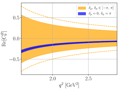
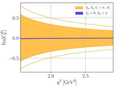
Fig. 1 illustrates the impact of the uncertainties from the unknown phases on real and imaginary parts of $C_{9}^{R}$ in the high $q^{2}$–region ($\sqrt{q^{2}}\geq 1.25$ GeV) for $D\to\pi\mu^{+}\mu^{-}$ decays. The phases $\delta_{\rho,\,\phi}$ give rise to huge uncertainties, shown by the yellow wider bands. As a result, even the sign of $C_{9}^{R}$ cannot be predicted. Once the phases are fixed, the residual uncertainties from $a_{\rho},a_{\phi}$, shown by the blue bands, are small. In addition, they could be reduced by improved measurements of $D\to PM$ and $M\to\ell^{+}\ell^{-}$ branching ratios. Darker shaded solid lines correspond to central values of input with strong phases fixed to $\delta_{\rho}=0$, $\delta_{\phi}=\pi$, consistent with the $SU(3)_{F}$ limit $\delta_{\rho}-\delta_{\phi}=\pi$.

Figure 1: Resonance contributions to the real part (plot to the left) and the imaginary part (plot to the right) of $C_{9}^{R}$ in the high $q^{2}$–region using the $D^{+}\to\pi^{+}$ parameters from Tab. 1. The wider yellow bands correspond to the uncertainties from strong phases $\delta_{\rho},\delta_{\phi}$ varied within $[-\pi,+\pi]$, whereas the smaller blue bands correspond to fixed strong phases $\delta_{\rho}=0,\delta_{\phi}=\pi$. Additional uncertainties arise from $a_{\rho},a_{\phi}$, and are included in the plots. The dashed curves illustrate the uncertainties in the case of $D^{0}\to\pi^{0}$ parameters.

II.3 Phenomenological $q^{2}$–distributions

The differential decay distribution of $D\to P\ell^{+}\ell^{-}$ can be written as Bobeth:2007dw

$$\begin{split}{\text{d}\Gamma\over\text{d}q^{2}}&={G_{F}^{2}\alpha_{e}^{2}\over 1024\pi^{5}m_{D}^{3}}\sqrt{\lambda_{DP}\biggl{(}1-{4m_{\ell}^{2}\over q^{2}}\biggr{)}}\,\biggl{\{}\biggr{.}\\ &\quad{2\over 3}\biggl{|}C_{9}+C_{9}^{R}+C_{7}{2m_{c}\over m_{D}+m_{P}}{f_{T}\over f_{+}}\biggr{|}^{2}\left(1+{2m_{\ell}^{2}\over q^{2}}\right)\lambda_{DP}f_{+}^{2}\\ &\quad+|C_{10}|^{2}\left[{2\over 3}\left(1-{4m_{\ell}^{2}\over q^{2}}\right)\lambda_{DP}f_{+}^{2}+{4m_{\ell}^{2}\over q^{2}}(m_{D}^{2}-m_{P}^{2})^{2}f_{0}^{2}\right]\\ &\quad+\left[|C_{S}|^{2}\left(1-{4m_{\ell}^{2}\over q^{2}}\right)+|C_{P}+C_{P}^{R}|^{2}\right]{q^{2}\over m_{c}^{2}}(m_{D}^{2}-m_{P}^{2})^{2}f_{0}^{2}\\ &\quad+{4\over 3}\left[|C_{T}|^{2}+|C_{T5}|^{2}\right]\left(1-{4m_{\ell}^{2}\over q^{2}}\right){q^{2}\over(m_{D}+m_{P})^{2}}\lambda_{DP}f_{T}^{2}\\ &\quad+8\,\text{Re}\left[\left(C_{9}+C_{9}^{R}+C_{7}{2m_{c}\over m_{D}+m_{P}}{f_{T}\over f_{+}}\right)C_{T}^{*}\right]{m_{\ell}\over m_{D}+m_{P}}\lambda_{DP}f_{+}f_{T}\\ &\quad+4\,\text{Re}\left[C_{10}\left(C_{P}+C_{P}^{R}\right)^{*}\right]{m_{\ell}\over m_{c}}(m_{D}^{2}-m_{P}^{2})^{2}f_{0}^{2}+16\,|C_{T}|^{2}\frac{m_{\ell}^{2}}{(m_{D}+m_{P})^{2}}\lambda_{DP}f_{T}^{2}\biggr{.}\biggr{\}}\end{split}$$ (7)

with $\lambda_{DP}=m_{D}^{4}+m_{P}^{4}+q^{4}-2m_{D}^{2}\,m_{P}^{2}-2m_{D}^{2}\,q^{2}-2m_{P}^{2}q^{2}\,$. To ease notation, here and in the following, all Wilson coefficients $C_{i}$, with the exception of the tensor ones, are understood as

$$C_{i}\to C_{i}+C_{i}^{\prime}\,.$$ (8)

We neglect the up-quark mass. The corresponding $D_{s}\to K\ell^{+}\ell^{-}$ decay distribution can be obtained by replacing $m_{D}\to m_{D_{s}}$, using $D_{s}\to K$ form factors $f_{+,0,T}$ and resonance parameters $a_{\rho,\,\phi,\,\eta,\,\eta^{\prime}}$ from Tab. 1. A detailed discussion of the form factors can be found in App. A.

In this work we give predictions for $D^{+}\to\pi^{+}\ell\ell^{(\prime)}$ observables. Predictions for $D^{0}\to\pi^{0}\ell\ell^{(\prime)}$ decays are, within uncertainties, the same as for $D^{+}\to\pi^{+}\ell\ell^{(\prime)}$ decays except for branching ratios, which need to be rescaled by the ratio of lifetimes, $\tau(D^{+})/\tau(D^{0})=2.54$ Tanabashi:2018oca .

Figure 2: The differential SM branching fractions of $D^{+}\to\pi^{+}\mu^{+}\mu^{-}$ (plot to the left) and $D_{s}^{+}\to K^{+}\mu^{+}\mu^{-}$ (plot to the right) decays. Yellow (blue) bands show pure resonant (short-distance) contributions. The band widths represent theoretical uncertainties of hadronic form factors, resonance parameters and $\mu_{c}$. Darker shaded thin curves represent all parameters set to their central values including $\delta_{\rho}=0$ and $\delta_{\phi}=\pi$ (solid) and $\delta_{\rho}=\delta_{\phi}=0$ (dashed). For the experimental limit by LHCb Aaij:2013sua see Eq. (9).

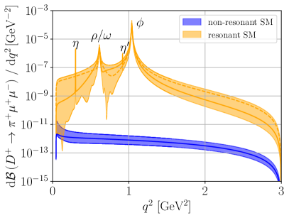
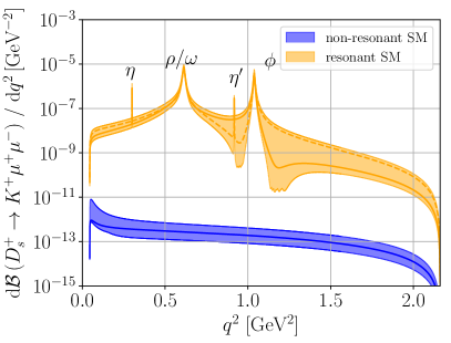
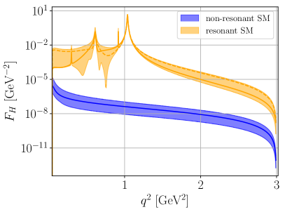
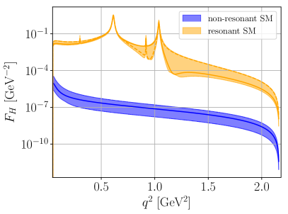
In Fig. 2 we show the pure non-resonant $q^{2}$–spectra determined by the SM short-distance $C_{7,9}^{\rm eff}$ coefficients (lower, blue curves) and the pure resonant ones determined by $C_{9,P}^{R}$ (yellow, wiggly curves). The non-resonant contribution is suppressed by several orders of magnitude with respect to the resonant one and negligible in the SM. The band width represents theoretical uncertainties of the form factors, the resonance parameters $a_{M}$ with corresponding phases $\delta_{M}$, see Eq. (6), and the scale $\mu_{c}$. The largest uncertainty stems from the unknown phases $\delta_{M}$, an effect which is pronounced through resonance interference.

The uncertainties from the strong phases $\delta_{M}$ are highly dependent on the values of the $a_{M}$. One can infer from Fig. 2 that the $D$–mode has huge uncertainties at low $q^{2}$ and around the $\rho/\omega$ peak, and it has much smaller uncertainties and more stable behavior above the $\phi$ mass, while for the $D_{s}$–mode the situation is the opposite. The reason for this difference is the numerical values and hierarchy of $a_{\rho}$ and $a_{\phi}$ (see Tab. 1). Although the tiny uncertainty band in the low $q^{2}$–region of the $D_{s}$–mode looks promising for testing new physics, we stress that the uncertainty band width can change with future measurements of the $D_{s}\to KM$ and $M\to\ell^{+}\ell^{-}$ branching ratios.

III Beyond the Standard Model

BSM effects in the $c\to u\ell\ell^{(\prime)}$ transition are discussed in a model-independent way. In Sec. III.1 we update the constraints on the Wilson coefficients coming from $D^{+}\to\pi^{+}\mu^{+}\mu^{-}$ and $D^{0}\to\mu^{+}\mu^{-}$ branching ratios and discuss the BSM sensitivity of $\mathcal{B}(D\to P\ell^{+}\ell^{-}$) at high $q^{2}$. In Sec. III.2 lepton universality tests are considered. Null tests of the SM based on the angular distributions are discussed in Sec. III.3. CP–asymmetries and their sensitivity to BSM benchmark values is analyzed in Sec III.4. In Sec. III.5 lepton flavor violating $c\to ue^{\pm}\mu^{\mp}$ decays are discussed.

III.1 Updated constraints on Wilson coefficients

Using the experimental limits on the branching fraction of $D^{+}\to\pi^{+}\mu^{+}\mu^{-}$ in high and full $q^{2}$–regions at 90% CL Aaij:2013sua ,

$$\begin{split}\mathcal{B}(D^{+}\to\pi^{+}\mu^{+}\mu^{-})|_{{\rm full}~{}q^{2}}&<7.3\times 10^{-8}\quad(250\,{\rm MeV}\leq\sqrt{q^{2}}\leq m_{D^{+}}-m_{\pi^{+}})\,,\\ \mathcal{B}(D^{+}\to\pi^{+}\mu^{+}\mu^{-})|_{{\rm high}~{}q^{2}}&<2.6\times 10^{-8}\quad(\sqrt{q^{2}}\geq 1.25~{}{\rm GeV})\,,\end{split}$$ (9)

and neglecting the SM contributions, we obtain the following constraints on the BSM Wilson coefficients in the full $q^{2}$–region,

$$\begin{split}&1.2|C_{7}|^{2}+1.2|C_{9}|^{2}+1.2|C_{10}|^{2}+2.4|C_{S}|^{2}+2.5|C_{P}|^{2}+0.4|C_{T}|^{2}+0.3|C_{T5}|^{2}\\ &+0.3\,\mathrm{Re}[C_{9}C_{T}^{*}]+1.0\,\mathrm{Re}[C_{10}C_{P}^{*}]+2.4\,\mathrm{Re}[C_{7}C_{9}^{*}]+0.6\,\mathrm{Re}[C_{7}C_{T}^{*}]\lesssim 1\,.\end{split}$$ (10)

and in the high $q^{2}$–region,

$$\begin{split}&0.6|C_{7}|^{2}+0.7|C_{9}|^{2}+0.8|C_{10}|^{2}+4.4|C_{S}|^{2}+4.5|C_{P}|^{2}+0.4|C_{T}|^{2}+0.4|C_{T5}|^{2}\\ &+0.3\,\mathrm{Re}[C_{9}C_{T}^{*}]+1.1\,\mathrm{Re}[C_{10}C_{P}^{*}]+1.4\,\mathrm{Re}[C_{7}C_{9}^{*}]+0.3\,\mathrm{Re}[C_{7}C_{T}^{*}]\lesssim 1\,,\end{split}$$ (11)

We find good agreement between Eq. (11), in the limit when only one $C_{i}$ is present, and Ref. Fajfer:2015mia . The limits (10), (11) are also consistent with the fact that in all $D\to P\ell^{+}\ell^{-}$ distributions the leptonic vector current is probed only through the combination

$$C_{9}+C_{9}^{R}+C_{9}^{\prime}+\gamma(C_{7}+C_{7}^{\prime})\,,$$ (12)

with $\gamma={2m_{c}\over m_{D}+m_{P}}{f_{T}\over f_{+}}$, which numerically is around one in the full $q^{2}$–region, $\gamma\approx 1$, as shown in App. A. Present bounds on dipole operators from $D\to\rho\gamma$ Abdesselam:2016yvr ; deBoer:2017que are in agreement with (10), (11).

The numerical coefficients in Eqs. (10) and (11) are smaller than the corresponding ones in Eqs. (29) and (30) of Ref. deBoer:2015boa . This difference is caused by the $D\to\pi$ form factors, for which we use new lattice results Lubicz:2017syv ; Lubicz:2018rfs (for details, see App. A). This in particular affects $f_{T}$ and hence the available space for NP in $C_{T,T5}$ and $C_{7}^{(\prime)}$.

Note that in Eqs. (10) and (11) we neglected the contributions from $C_{9,\,P}^{R}$. Taking them into account, we obtain one additional constant term plus several interference terms proportional to Re$[C_{i}]$ and Im$[C_{i}]$ on the left-hand side of Eqs. (10) and (11). When varying strong phases, the constant term turns out to be smaller than 0.1. The largest numerical coefficients of the interference terms can vary in the full $q^{2}$–region within [-0.1, 0.1] and [-0.2, 0.2] for $C_{9}$ and $C_{7}$, respectively, whereas at high $q^{2}$ the corresponding ranges turn out to be larger, about a factor $\sim 2$ to 5. Despite being less tight we use in the following the constraint from the $D^{+}\to\pi^{+}\mu^{+}\mu^{-}$ branching fraction in the high $q^{2}$–region as it is the best available bound we trust, since no extrapolations of signal have been included, in contrast to the full $q^{2}$–region. One may wonder whether Wilson coefficients as large as order one of $|\Delta c|=|\Delta u|=1$ four-fermion operators are constrained from high-$p_{T}$ searches. While a dedicated analysis for up-sector flavor changing neutral currents (FCNCs) is currently not available, constraints derived from $36.1\,\rm{fb}^{-1}$ ATLAS data on semileptonic operators with two charm singlets or two second generation quark doublets Greljo:2017vvb are close to probing the range allowed by charm decays into muons, and are somewhat stronger for electrons.

Further constraints on $C_{10,S,P}^{(\prime)}$ can be obtained from the $D^{0}\to\ell^{+}\ell^{-}$ branching ratio

$$\begin{split}\mathcal{B}(D^{0}\to\ell^{+}\ell^{-})&=\tau_{D}{G_{F}^{2}\alpha_{e}^{2}m_{D}^{5}f_{D}^{2}\over 64\pi^{3}m_{c}^{2}}\sqrt{1-{4m_{\ell}^{2}\over m_{D}^{2}}}\left[\left(1-{4m_{\ell}^{2}\over m_{D}^{2}}\right)|C_{S}-C_{S}^{\prime}|^{2}\right.\\ &\quad\left.+\left|C_{P}-C_{P}^{\prime}+{2m_{\ell}m_{c}\over m_{D}^{2}}(C_{10}-C_{10}^{\prime})\right|^{2}\right]\,.\end{split}$$ (13)

The upper limit $\mathcal{B}(D^{0}\to\mu^{+}\mu^{-})<6.2\times 10^{-9}$ at 90% CL Aaij:2013cza gives

$$|C_{S}-C_{S}^{\prime}|^{2}+|C_{P}-C_{P}^{\prime}+0.1(C_{10}-C_{10}^{\prime})|^{2}\lesssim 0.007\,.$$ (14)

In addition, tensor Wilson coefficients are constrained by the leptonic decays as they induce scalar ones from renormalization group running Gonzalez-Alonso:2017iyc . In the subsequent analysis we use $|C_{S,P}|\simeq 0.1$ and $|C_{i}|\simeq 0.5$ for all other NP Wilson coefficients as benchmark values. An exception is Sec. III.4 on CP-violating effects, which are subject to model-dependent, generically stronger $D$-mixing constraints, see App. B for details. In the following $C_{i(j)}$ stands for "$C_{i}$ or $C_{j}$".

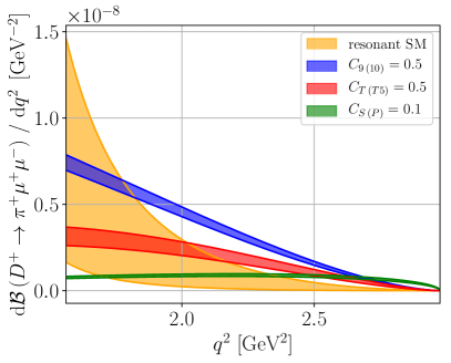
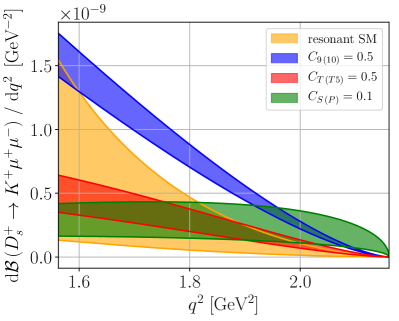
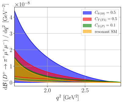
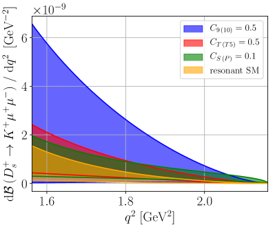
In Fig. 3 and Tab. 2 we illustrate the NP sensitivity of the $D_{(s)}^{+}\to\pi(K)^{+}\mu^{+}\mu^{-}$ differential and integrated branching fractions, respectively, at high $q^{2}$. Results for the intermediate resonance region and at low $q^{2}$ are not given due to sizable theoretical uncertainties, see, for instance, Fig. 2. The largest deviations from the SM in the branching ratios are possible with (axial)-vector operators $O_{9,10}^{(\prime)}$, followed by tensors $O_{T,T5}$ and (pseudo)-scalar operators $O_{S,P}^{(\prime)}$. An exception to this arises close to the endpoint, where $O_{S,P}^{(\prime)}$ effects can become the largest as they do have one power of the Källen function $\lambda_{DP}$ less in Eq. (7). While there can be NP distributions in excess of the SM one shown by the yellow band, the window for NP is small. In view of the sizable hadronic uncertainties NP branching ratios need to be close to the present experimental upper limit to support a BSM interpretation without further input or data. Taking the resonances into account enhances the BSM branching ratios and makes them more uncertain, see the lower plots in Fig. 3 (resonances plus NP), in comparison to the upper plots of Fig. 3 (pure NP). The sensitivity to BSM dipole operators $O_{7}^{(\prime)}$ is similar to the one of $O_{9}^{(\prime)}$, see Eq. (12), and therefore not shown.

Figure 3: The differential branching fractions in the SM and in three BSM scenarios in the high $q^{2}$–region for $D^{+}\to\pi^{+}\mu^{+}\mu^{-}$ (plots to the left) and $D_{s}^{+}\to K^{+}\mu^{+}\mu^{-}$ (plots to the right). Orange bands correspond to the pure resonant contributions. The band width represents theoretical uncertainties, where we distinguish between pure BSM contributions (upper plots) and BSM benchmarks including interference with the SM resonance contributions, such that the variation of the strong phases also effects the BSM predictions (lower plots). Predictions for BSM coefficients $C_{7}^{(\prime)}$ are similar to those of $C_{9}^{(\prime)}$ (cf. Eq. (12)), and not shown.

Table 2: Integrated branching fractions in the high $q^{2}$–bin ($\sqrt{q^{2}}\geq 1.25$ GeV) in the SM and in the NP benchmark scenarios as in Fig. 3. In the third to sixth column, upper entries correspond to NP-only branching ratios while for the lower entries the resonance contributions are taken into account.

$\mathcal{B}|_{\text{high}\,q^{2}}\,\times 10^{9}$			SM			$C_{9\,(10)}=0.5$			$C_{S\,(P)}=0.1$			$C_{T\,(T5)}=0.5$			$C_{9}=\pm C_{10}=0.5$
$D^{+}\to\pi^{+}\mu^{+}\mu^{-}$			$0.3\ldots 3.0$			$4.5\pm 0.3$			$1.1\pm 0.1$			$2.6\pm 0.4$			$9.4\pm 0.6$
						$7.8\pm 7.4$			$2.9\pm 1.4$			$5.0\pm 2.9$			$12.6\pm 7.7$
$D_{s}^{+}\to K^{+}\mu^{+}\mu^{-}$			$0.03\ldots 0.3$			$0.40\pm 0.05$			$0.15\pm 0.07$			$0.15\pm 0.05$			$0.8\pm 0.1$
						$0.8\pm 0.7$			$0.3\pm 0.2$			$0.4\pm 0.3$			$1.2\pm 0.8$

III.2 Testing lepton universality

Lepton universality can be probed in semileptonic decays with the ratios Fajfer:2015mia ; deBoer:2018buv

$$R_{P}^{D}={\displaystyle{\int_{q_{\rm min}^{2}}^{q_{\rm max}^{2}}{\text{d}\mathcal{B}(D\to P\mu^{+}\mu^{-})\over\text{d}q^{2}}\text{d}q^{2}}\over\displaystyle{\int_{q_{\rm min}^{2}}^{q_{\rm max}^{2}}{\text{d}\mathcal{B}(D\to Pe^{+}e^{-})\over\text{d}q^{2}}\text{d}q^{2}}}\,.$$ (15)

Here, $q_{\rm min}^{2}$ ($q_{\rm max}^{2}$) denotes the lower (upper) dilepton mass cut; to ensure maximal cancellation of hadronic uncertainties and hence a controlled SM prediction near unity it is crucial that the cuts for electron and muon modes are identical Hiller:2003js . Assuming that NP contributes only to the muon mode, we present in Tabs. 3 and 4 the predicted ranges of $R_{\pi}^{D}$ and $R_{K}^{D_{s}}$, respectively, in the full, low and high $q^{2}$–integrated intervals. As for the resonance parametrization, we use the same $C_{9,P}$ for electron and muon modes. Due to poor knowledge of the resonances’ behavior, the predictions for the low $q^{2}$–region ($\sqrt{q^{2}}\in[250,525]$ MeV) have sizable uncertainties and we only give the order of magnitude of the largest values found. The main uncertainty comes from the phases $\delta_{\rho,\,\phi,\,\eta}$ which are varied within $-\pi$ and $\pi$, while the uncertainties due to hadronic form factors are of the order of few percent. Integration over the full $q^{2}$–interval gives ratios $R_{\pi}^{D}$ and $R_{K}^{D_{s}}$ which are insensitive to NP. On the other hand, in the high $q^{2}$–region NP can induce significant effects. BSM effects in the low $q^{2}$–region can be huge in the $D$–mode, however, there are large uncertainties.

Table 3: $R_{\pi}^{D}$ (15) in the SM and in NP scenarios for different $q^{2}$–bins. Ranges correspond to uncertainties from form factors and resonance parameters. Due to large uncertainties at low $q^{2}$ in some cases only the order of magnitude of the largest values is given.

	SM	$|C_{9}|=0.5$	$|C_{10}|=0.5$	$|C_{9}|=\pm|C_{10}|=0.5$	$|C_{S\,(P)}|=0.1$	$|C_{T}|=0.5$	$|C_{T5}|=0.5$
full $q^{2}$	$1.00\pm\mathcal{O}(\%)$	SM-like	SM-like	SM-like	SM-like	SM-like	SM-like
low $q^{2}$	$0.95\pm\mathcal{O}(\%)$	$\mathcal{O}(100)$	$\mathcal{O}(100)$	$\mathcal{O}(100)$	$0.9\ldots 1.4$	$\mathcal{O}(10)$	$1.0\ldots 5.9$
high $q^{2}$	$1.00\pm\mathcal{O}(\%)$	$0.2\ldots 11$	$3\ldots 7$	$2\ldots 17$	$1\ldots 2$	$1\ldots 5$	$2\ldots 4$

Table 4: $R_{K}^{D_{s}}$ (15) in the SM and in NP scenarios for different $q^{2}$–bins, see Tab. 3 and text.

	SM	$|C_{9}|=0.5$	$|C_{10}|=0.5$	$|C_{9}|=\pm|C_{10}|=0.5$	$|C_{S\,(P)}|=0.1$	$|C_{T}|=0.5$	$|C_{T5}|=0.5$
full $q^{2}$	$1.00\pm\mathcal{O}(\%)$	SM-like	SM-like	SM-like	SM-like	SM-like	SM-like
low $q^{2}$	$0.94\pm\mathcal{O}(\%)$	$0.1\ldots 3.0$	$1.3\ldots 1.5$	$0.5\ldots 3.6$	SM-like	$0.7\ldots 1.2$	SM-like
high $q^{2}$	$1.00\pm\mathcal{O}(\%)$	$0.2\ldots 16$	$3\ldots 11$	$2\ldots 26$	$1.5\ldots 3.7$	$1\ldots 6$	$1.6\ldots 4.1$

III.3 Angular observables

The double differential distribution of $D\to P\ell^{+}\ell^{-}$ decays Bobeth:2007dw

$${\text{d}^{2}\Gamma\over\text{d}q^{2}\,\text{d}\cos\theta}=a(q^{2})+b(q^{2})\cos\theta+c(q^{2})\cos^{2}\theta\,,$$ (16)

where $\theta$ denotes the angle between the $\ell^{-}$–momentum and the $P$–momentum in the dilepton rest frame, offers the measurement of two angular observables: The lepton forward-backward asymmetry,

$$\begin{split}A_{\rm FB}(q^{2})&={1\over\Gamma}\left[\int_{0}^{1}-\int_{-1}^{0}\right]{\text{d}^{2}\Gamma\over\text{d}q^{2}\text{d}\cos\theta}\text{d}\cos\theta={b(q^{2})\over\Gamma}={1\over\Gamma}{G_{F}^{2}\alpha_{e}^{2}\over 512\pi^{5}m_{D}^{3}}\lambda_{DP}\biggl{(}1-{4m_{\ell}^{2}\over q^{2}}\biggr{)}\biggl{\{}\biggr{.}\\ &\quad\text{Re}\left[\left(C_{9}+C_{9}^{R}+C_{7}{2m_{c}\over m_{D}+m_{P}}{f_{T}\over f_{+}}\right)C_{S}^{*}\right]{m_{\ell}\over m_{c}}f_{+}+2\text{Re}\left[C_{10}C_{T5}^{*}\right]{m_{\ell}\over m_{D}+m_{P}}f_{T}\\ &\quad+\text{Re}\left[C_{S}C_{T}^{*}+\left(C_{P}+C_{P}^{R}\right)C_{T5}^{*}\right]{q^{2}\over m_{c}(m_{D}+m_{P})}f_{T}\biggl{.}\biggr{\}}(m_{D}^{2}-m_{P}^{2})f_{0}\,,\end{split}$$ (17)

and the “flat” term,

$$\begin{split}F_{H}(q^{2})&={2\over\Gamma}[a(q^{2})+c(q^{2})]={1\over\Gamma}{G_{F}^{2}\alpha_{e}^{2}\over 1024\pi^{5}m_{D}^{3}}\sqrt{\lambda_{DP}\biggl{(}1-{4m_{\ell}^{2}\over q^{2}}\biggr{)}}\,\biggl{\{}\biggr{.}\\ &\quad\biggl{|}C_{9}+C_{9}^{R}+C_{7}{2m_{c}\over m_{D}+m_{P}}{f_{T}\over f_{+}}\biggr{|}^{2}{4m_{\ell}^{2}\over q^{2}}\lambda_{DP}f_{+}^{2}+|C_{10}|^{2}{4m_{\ell}^{2}\over q^{2}}(m_{D}^{2}-m_{P}^{2})^{2}f_{0}^{2}\\ &\quad+\left[|C_{S}|^{2}\left(1-{4m_{\ell}^{2}\over q^{2}}\right)+|C_{P}+C_{P}^{R}|^{2}\right]{q^{2}\over m_{c}^{2}}(m_{D}^{2}-m_{P}^{2})^{2}f_{0}^{2}\\ &\quad+4\,\left[|C_{T}|^{2}+|C_{T5}|^{2}\right]\left(1-{4m_{\ell}^{2}\over q^{2}}\right){q^{2}\over(m_{D}+m_{P})^{2}}\lambda_{DP}f_{T}^{2}\\ &\quad+8\,\text{Re}\left[\left(C_{9}+C_{9}^{R}+C_{7}{2m_{c}\over m_{D}+m_{P}}{f_{T}\over f_{+}}\right)C_{T}^{*}\right]{m_{\ell}\over m_{D}+m_{P}}\lambda_{DP}f_{+}f_{T}\\ &\quad+4\,\text{Re}\left[C_{10}\left(C_{P}+C_{P}^{R}\right)^{*}\right]{m_{\ell}\over m_{c}}(m_{D}^{2}-m_{P}^{2})^{2}f_{0}^{2}+16\,|C_{T}|^{2}\frac{m_{\ell}^{2}}{(m_{D}+m_{P})^{2}}\lambda_{DP}f_{T}^{2}\biggr{.}\biggr{\}}\,.\end{split}$$ (18)

both with normalization to the $q^{2}$-integrated decay rate,

$$\Gamma=\Gamma(q^{2}_{\rm min},q^{2}_{\rm max})=\int_{q^{2}_{\rm min}}^{q^{2}_{\rm max}}{\text{d}\Gamma\over\text{d}q^{2}}\text{d}q^{2}=2\int_{q^{2}_{\rm min}}^{q^{2}_{\rm max}}\left(a(q^{2})+\frac{c(q^{2})}{3}\right)\,\text{d}q^{2}\,,$$ (19)

with integration limits depending on the $q^{2}$–bin. Since the scalar and pseudotensor operators are absent in the SM, $A_{\rm FB}$ constitutes a null test . We find that in the SM $F_{H}(D\to\pi\mu^{+}\mu^{-})$ is $\mathcal{O}(10^{-3})$ at low $q^{2}$, whereas $F_{H}(D_{s}\to K\mu^{+}\mu^{-})$ is $\mathcal{O}(10^{-2})$ and both are even smaller at high $q^{2}$, see Fig. 4. $F_{H}(D_{(s)}\to\pi(K)e^{+}e^{-})$ in the SM is even further suppressed. We learn that $F_{H}$ is yet another a very promising null test of the SM, sensitive to NP in (pseudo)-scalar and tensor operators.

Figure 4: The SM contributions to $F_{H}(q^{2})$ given in Eq. (18) for $D^{+}\to\pi^{+}\mu^{+}\mu^{-}$ (plot to the left) and $D_{s}^{+}\to K^{+}\mu^{+}\mu^{-}$ (plot to the right) decays, see Fig. 2.

Figure 5: The forward-backward asymmetry $A_{\rm FB}$ (upper plots) and $F_{H}$ (lower plots) in the high–$q^{2}$ region in different BSM scenarios for $D^{+}\to\pi^{+}\mu^{+}\mu^{-}$ (plots to the left) and $D_{s}^{+}\to K^{+}\mu^{+}\mu^{-}$ (plots to the right).

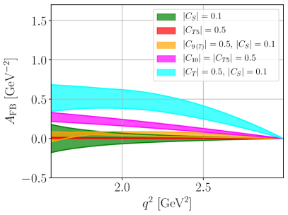
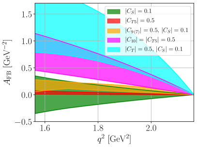
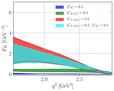
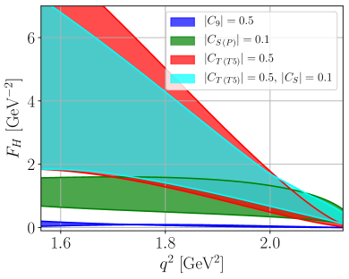
In Fig. 5 we show $A_{\rm FB}$ and $F_{H}$ in different NP scenarios for $D^{+}\to\pi^{+}\mu^{+}\mu^{-}$ (plots to the left) and $D_{s}^{+}\to K^{+}\mu^{+}\mu^{-}$ (plots to the right) at high $q^{2}$, that is, $q^{2}_{\rm min}=(1.25\,\mbox{GeV})^{2}$ and $q^{2}_{\rm max}=(m_{D}-m_{P})^{2}$. The band width represents theoretical uncertainties. One can see that $A_{\rm FB}$ is mostly sensitive to the combinations of tensor and (pseudo)scalar operators, while it is significantly suppressed if only scalar or pseudotensor structure is present. The latter effect comes from interference terms, $C_{9}^{R}C_{S}^{*}$ and $C_{P}^{R}C_{T5}^{*}$, which are suppressed by the light lepton mass and small $\eta$-resonance contribution to $C_{P}^{R}$, respectively. The flat term turns out to be sensitive to the (pseudo)scalar and especially to the (pseudo)tensor operators. The effect of simultaneous presence of scalar and tensor contributions (in cyan) is essentially indistinguishable from the one induced by pure (pseudo)tensor (in red) structure. However, large effects in both $F_{H}$ and $A_{\rm FB}$ would be a signal of tensor and scalar nature of NP. In Sec. IV we zoom into Fig. 5, and discuss in more detail possible signals of NP induced predominantly by (axial-)vector contributions. The normalization of angular observables has significant impact on the shape of the distributions. Choosing $d\Gamma/dq^{2}$, as in Sahoo:2017lzi , instead of $\Gamma$ (19), results in markedly different behavior for $F_{H}$ near the endpoint $q^{2}\to(m_{D}-m_{P})^{2}$, where cancellations can occur.

III.4 CP–asymmetry

Another promising observable to probe NP is the CP–asymmetry, defined as Fajfer:2012nr ; deBoer:2015boa

$$A_{\rm CP}(q^{2})={1\over\Gamma+\overline{\Gamma}}\left({\text{d}\Gamma\over\text{d}q^{2}}-{\text{d}\overline{\Gamma}\over\text{d}q^{2}}\right)\,,$$ (20)

where $\overline{\Gamma}$ denotes the decay rate of the CP–conjugated mode, defined with $q^{2}$-bin dependence as $\Gamma$ in Eq. (19). The difference of the differential rates can be written as

$$\begin{split}{\text{d}\Gamma\over\text{d}q^{2}}-{\text{d}\overline{\Gamma}\over\text{d}q^{2}}&={G_{F}^{2}\alpha_{e}^{2}\over 256\pi^{5}m_{D}^{3}}\sqrt{\lambda_{DP}\biggl{(}1-{4m_{\ell}^{2}\over q^{2}}\biggr{)}}\,\biggl{\{}\biggr{.}\\ &\quad{2\over 3}\,\text{Im}\left[C_{9}+2C_{7}{m_{c}\over m_{D}+m_{P}}{f_{T}\over f_{+}}\right]\text{Im}\left[C_{9}^{R}\right]\left(1+{2m_{\ell}^{2}\over q^{2}}\right)\lambda_{DP}f_{+}^{2}\\ &\quad+\text{Im}\left[C_{P}\right]\text{Im}\left[C_{P}^{R}\right]{q^{2}\over m_{c}^{2}}(m_{D}^{2}-m_{P}^{2})^{2}f_{0}^{2}\\ &\quad+4\,\text{Im}\left[C_{T}\right]\text{Im}\left[C_{9}^{R}\right]{m_{\ell}\over m_{D}+m_{P}}\lambda_{DP}f_{+}f_{T}\\ &\quad+2\,\text{Im}\left[C_{10}\right]\text{Im}\left[C_{P}^{R}\right]{m_{\ell}\over m_{c}}(m_{D}^{2}-m_{P}^{2})^{2}f_{0}^{2}\biggr{.}\biggr{\}}\,.\end{split}$$ (21)

$A^{\rm SM}_{\rm CP}$ is determined by the first term in Eq. (21) and remains tiny due to small phases of the CKM factors in $C_{9}$, see Eq. (4). Existing bounds from $A_{\rm CP}(D^{0}\to\rho^{0}\gamma)=0.056\pm 0.152\pm 0.006$ Abdesselam:2016yvr do not provide further constraints on $C_{7}^{(\prime)}$ beyond the ones from branching ratio measurements deBoer:2017que . Naïve T-odd CP-asymmetries from angular distributions in $D\to\pi\pi\mu^{+}\mu^{-}$ decays can probe CP-phases even for vanishing strong phases. First experimental studies are at the ${\cal{O}}(10\,\%)$ level Aaij:2018fpa which is about where sensitivity to BSM physics starts deBoer:2018buv .

Figure 6: The CP–asymmetry in $D^{+}\to\pi^{+}\mu^{+}\mu^{-}$ (plots to the left) and $D_{s}^{+}\to K^{+}\mu^{+}\mu^{-}$ (plots to the right) decays around the $\phi$ resonance $[(m_{\phi}-5\Gamma_{\phi})^{2},(m_{\phi}+5\Gamma_{\phi})^{2}]$ (upper plots) and in the high–$q^{2}$ region (lower plots) for different values of $\delta_{\phi}=0,\pm\pi/2,\pi$ and $C_{9}=0.1\exp(\text{i}\,\pi/4)$. The uncertainties are due to the other strong phases $(\delta_{\rho},\,\delta_{\eta})$, the form factors, as well as the charm quark mass $m_{c}$.

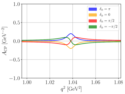
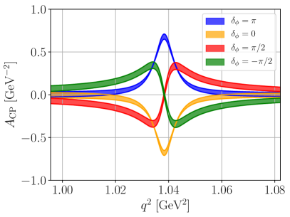
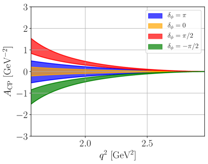
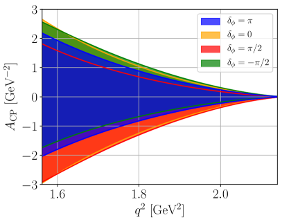
For a sizable (T-even) CP–asymmetry, enhanced strong phases and therefore resonance effects are instrumental Fajfer:2012nr . In Fig. 6 we show $A_{\rm CP}$ in the $\phi$–region (upper plots) and at high $q^{2}$ (lower plots) for $C_{9}=0.1\exp(\text{i}\,\pi/4)$ and different values of $\delta_{\phi}$. The band width corresponds to the $1\sigma$ uncertainty due to $m_{c}$, form factors and resonance parameters ($\delta_{\rho,\eta}$, varied within $-\pi$ and $\pi$). NP effects in $C_{T}$ and $C_{P,10}$ are suppressed by the light lepton mass and the completely negligible $\text{Im}[C_{P}^{R}(q^{2}\simeq m_{\phi}^{2})]$ respectively. We learn from Fig. 6 that irrespective of the value of $\delta_{\phi}$, sizable BSM effects occur making this observable promising for NP searches. Except for $D_{s}\to K\ell^{+}\ell^{-}$ at high $q^{2}$, $A_{\rm CP}$ has rather small uncertainties and is useful to extract strong and weak parameters. Note that $A_{\rm CP}$ can change its sign around $q^{2}\sim m_{\phi}^{2}$ and hence, to avoid a vanishing integrated asymmetry, binning is required. Due to the way Eq. (12) with which leptonic vector contributions enter $D\to P\ell^{+}\ell^{-}$ decays, $A_{\rm CP}$ has similar sensitivity to BSM effects from $C_{7}^{(\prime)}$ than from $C_{9}^{(\prime)}$.

Similar to the behavior observed in the angular observables $F_{H}$ and $A_{\rm FB}$, BSM effects in $A_{\rm CP}$ in the $D_{s}\to K\ell^{+}\ell^{-}$ mode are enhanced relative to the $D\to\pi\ell^{+}\ell^{-}$ one, due to the smaller decay rate of the former, caused predominantly by kinematics.

III.5 Lepton flavor violation

To discuss LFV in $c\to u\ell^{-}\ell^{\prime+}$ ($\ell\neq\ell^{\prime}$) decays we introduce the following effective Hamiltonian,

$$\mathcal{H}_{\text{eff}}^{\rm LFV}=-{4G_{F}\over\sqrt{2}}{\alpha_{e}\over 4\pi}\sum_{i}\left(K_{i}^{(\ell\ell^{\prime})}O_{i}^{(\ell\ell^{\prime})}+K_{i}^{\prime\,(\ell\ell^{\prime})}O_{i}^{\prime\,(\ell\ell^{\prime})}\right)\,,$$ (22)

where the $K_{i}^{(\prime)}$ denote Wilson coefficients and the operators $O_{i}^{(\prime)}$ read as

$$O_{9}^{(\ell\ell^{\prime})}=(\overline{u}_{L}\gamma_{\mu}c_{L})(\overline{\ell}\gamma^{\mu}\ell^{\prime})\,,\quad\quad O_{9}^{\prime\,(\ell\ell^{\prime})}=(\overline{u}_{R}\gamma_{\mu}c_{R})(\overline{\ell}\gamma^{\mu}\ell^{\prime})\,,$$ (23)

with other operators from Eq. (2) defined in similar way by changing flavor in lepton currents. Note that there is no $O_{7}^{(\prime)}$ contribution since the photon does not couple to different lepton flavors.

The differential distribution for the LFV decays $D\to Pe^{\pm}\mu^{\mp}$ is given as

$$\begin{split}{\mathrm{d}\Gamma(D\to Pe^{\pm}\mu^{\mp})\over\mathrm{d}q^{2}}&={G_{F}^{2}\alpha_{e}^{2}\over 1024\pi^{5}m_{D}^{3}}\sqrt{\lambda_{DP}}\bigg{\{}\frac{2}{3}\left(|K_{9}|^{2}+|K_{10}|^{2}\right)\lambda(m_{D}^{2},m_{P}^{2},q^{2})f_{+}^{2}\\ &+\left(|K_{S}|^{2}+|K_{P}|^{2}\right){q^{2}\over m_{c}^{2}}(m_{D}^{2}-m_{P}^{2})^{2}f_{0}^{2}\\ &+\frac{4}{3}\left(|K_{T}|^{2}+|K_{T5}|^{2}\right){q^{2}\over(m_{D}+m_{P})^{2}}\lambda_{DP}f_{T}^{2}\\ &+2\mathrm{Re}\left[\pm K_{9}K_{S}^{*}+K_{10}K_{P}^{*}\right]{m_{\mu}\over m_{c}}(m_{D}^{2}-m_{P}^{2})^{2}f_{0}^{2}\\ &+4\mathrm{Re}\left[K_{9}K_{T}^{*}\pm K_{10}K_{T5}^{*}\right]{m_{\mu}\over m_{D}+m_{P}}\lambda_{DP}f_{+}f_{T}\bigg{\}}+\mathcal{O}\left(m_{\mu}^{2}\right)\,,\end{split}$$ (24)

where $K_{i}=K_{i}^{(\mu e)}+K_{i}^{\prime\,(\mu e)}$ for $D\to Pe^{+}\mu^{-}$ and $K_{i}=K_{i}^{(e\mu)}+K_{i}^{\prime\,(e\mu)}$ for $D\to Pe^{-}\mu^{+}$. Here we neglected the electron mass.

Similarly to Eq. (10), we obtain the following constraints on the LFV Wilson coefficients using the 90% C.L. upper limits $\mathcal{B}(D^{+}\to\pi^{+}e^{+}\mu^{-})<2.9\times 10^{-6}$ and $\mathcal{B}(D^{+}\to\pi^{+}e^{-}\mu^{+})<3.6\times 10^{-6}$ Lees:2011hb :

$$\begin{split}&1.3\,\big{(}|K_{9}|^{2}+|K_{10}|^{2}\big{)}+2.6\,\big{(}|K_{S}|^{2}+|K_{P}|^{2}\big{)}+0.4\,\big{(}|K_{T}|^{2}+\big{|}K_{T5}\big{|}^{2}\big{)}+\\ &0.5\,\mathrm{Re}\big{[}K_{10}K_{P}^{*}\pm K_{9}K_{S}^{*}\big{]}+0.3\,\mathrm{Re}\big{[}K_{9}K_{T}^{*}\pm K_{10}K_{T5}^{*}\big{]}\lesssim 50\,.\end{split}$$ (25)

Tighter constraints on $K_{9,10,S,P}^{(\prime)}$ can be obtained from data on leptonic decays,

$$\begin{split}\mathcal{B}(D^{0}\to e^{\pm}\mu^{\mp})&=\tau_{D^{0}}{G_{F}^{2}\alpha_{e}^{2}m_{D}^{5}f_{D}^{2}\over 64\pi^{3}m_{c}^{2}}\left(1-{m_{\mu}^{2}\over m_{D}^{2}}\right)^{2}\bigg{\{}\left|K_{S}-K_{S}^{\prime}\pm{m_{\mu}m_{c}\over m_{D}^{2}}\left(K_{9}-K_{9}^{\prime}\right)\right|^{2}\\ &\quad+\left|K_{P}-K_{P}^{\prime}+{m_{\mu}m_{c}\over m_{D}^{2}}\left(K_{10}-K_{10}^{\prime}\right)\right|^{2}\bigg{\}}\,,\end{split}$$ (26)

with $K_{i}^{(\prime)}=K_{i}^{(\prime)(\mu e)}$ for $D^{0}\to e^{+}\mu^{-}$ and $K_{i}^{(\prime)}=K_{i}^{(\prime)(e\mu)}$ for $D^{0}\to e^{-}\mu^{+}$. Using $\mathcal{B}(D^{0}\to e^{\pm}\mu^{\mp})<1.3\times 10^{-8}$ @ 90% C.L. Aaij:2015qmj , we obtain

$$\big{|}K_{S}-K_{S}^{\prime}\pm 0.04\,\big{(}K_{9}-K_{9}^{\prime}\big{)}\big{|}^{2}+\big{|}K_{P}-K_{P}^{\prime}+0.04\,\big{(}K_{10}-K_{10}^{\prime}\big{)}\big{|}^{2}\lesssim 0.01\,.\\$$ (27)

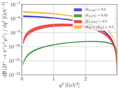
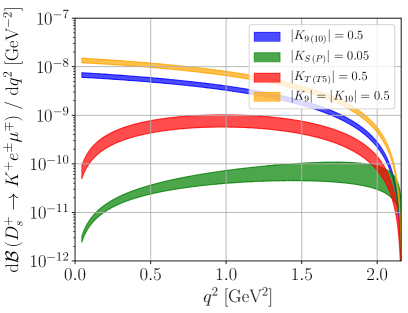
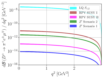
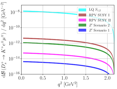
In Fig. 7 we present the differential branching fractions for LFV decays $D^{+}\to\pi^{+}e^{\pm}\mu^{\mp}$ and $D_{s}^{+}\to K^{+}e^{\pm}\mu^{\mp}$ for various NP Wilson coefficients allowed by Eqs. (25),(27). Since the resonant contributions are absent in the LFV processes, the uncertainties are due to the form factors and $m_{c}$, making the band widths in Fig. 7 significantly smaller than in Fig. 2. The difference in the shapes for vector and (pseudo)tensor/scalar structure allow to experimentally distinguish different operators and BSM scenarios.

Figure 7: The differential branching ratio of $D^{+}\to\pi^{+}e^{\pm}\mu^{\mp}$ (plot to the left) and $D_{s}^{+}\to K^{+}e^{\pm}\mu^{\mp}$ (plot to the right) decays in different LFV-BSM scenarios.

Note that there exists one opportunity to study $\tau$-couplings in leptonic charm decays,

$$\mathcal{B}(D^{0}\to e^{\pm}\tau^{\mp})=1.2\times 10^{-8}\,\left(\big{|}K_{S}-K_{S}^{\prime}\pm 0.7\,\big{(}K_{9}-K_{9}^{\prime}\big{)}\big{|}^{2}+\big{|}K_{P}-K_{P}^{\prime}+0.7\,\big{(}K_{10}-K_{10}^{\prime}\big{)}\big{|}^{2}\right)\,.\\$$ (28)

IV New Physics models for $c\to u\ell\ell$

We discuss signatures of leptoquarks in Sec. IV.1, and supersymmetry (SUSY) in Sec. IV.2. Contributions to $c\to u$ FCNCs in flavorful $Z^{\prime}$-models including explicit, anomaly-free realizations are worked out in Sec. IV.3.

In general, the models’ reach in rare charm decays is limited by kaon data, $D$-mixing and high-$p_{T}$ searches. Constraints from the down-sector can be escaped with contributions from singlet up-type quarks, giving rise to primed operators. Decoupling the doublets from kaon constraints requires assumptions on flavor. While this introduces model-dependence, it highlights the importance of joint charm and kaon studies and their impact on flavor model building. $D$-mixing constraints are most severe for the $Z^{\prime}$-models because, unlike in SUSY or leptoquark scenarios, meson mixing arises at tree-level, see App. B for details. We point out that the simultaneous presence of left-handed and right-handed couplings to quarks allows to avoid such constraints.

At the end of each model section we summarize how the model can signal NP in which observable from Sec. III, and refer to corresponding figures and tables.

IV.1 Leptoquark signatures

In order to bypass the constraints from the kaon sector in a most straightforward manner, we consider only the scalar leptoquarks $S_{1(2)}$ with right(left)-handed couplings and the vector ones $\widetilde{V}_{1,2}$, e.g. deBoer:2015boa ; Hiller:2016kry . The subscript "$1$" denotes $SU(2)_{L}$-singlets, whereas "$2$" denotes doublets. This precludes any (pseudo-)scalar or tensor operators, which otherwise would be induced by $S_{1,2}$, as well as (axial-)vector ones with left-handed quarks. We stress, however, that even small Wilson coefficients involving doublet quarks can signal NP in $A_{\rm CP}$, if CP-violating deBoer:2015boa . The interaction Lagrangian contributing to $c\to u\ell^{-}\ell^{\prime+}$ processes then reads Buchmuller:1986zs

$$\mathcal{L}_{\rm LQ}\supset\lambda_{S_{1}}^{ij}\,\overline{u}_{iR}^{c}l_{jR}\,S_{1}+\lambda_{S_{2}}^{ij}\,\overline{u}_{iR}L_{jL}\,S_{2}+\lambda_{\widetilde{V}_{1}}^{ij}\,\overline{u}_{iR}\gamma^{\mu}l_{jR}\,\widetilde{V}_{1\mu}+\lambda_{\widetilde{V}_{2}}^{ij}\,\overline{u}_{iR}^{c}\gamma^{\mu}L_{jL}\,\widetilde{V}_{2\mu}+{\rm c.c.}\,,$$ (29)

where $L_{L}$ denote lepton doublet and $l_{R},u_{R}$ lepton and up-type quark singlets; $i,j$ are the generation indices. Hypercharge-assignments of the leptoquarks can be read-off from (29); all leptoquarks are color-triplets. Charm signatures of $S_{2}$ have been studied in Fajfer:2015mia ; Sahoo:2017lzi and $\widetilde{V}_{1}$ in Fajfer:2015mia . Only $S_{2}^{5/3}$ and $\widetilde{V}_{2}^{1/3}$, and $S_{1}^{1/3}$, $\widetilde{V}_{1}^{5/3}$ mediate an interaction between up-type quarks and charged leptons, where superscripts indicate the electric charge. Using Fierz identities the Wilson coefficients of the $O_{9}^{\prime\,(\ell\ell^{\prime})}$ and $O_{10}^{\prime\,(\ell\ell^{\prime})}$ operators can be written as, e.g. deBoer:2015boa ,

$$\begin{split}K_{9}^{\prime\,(\ell\ell^{\prime})}&={\sqrt{2}\pi\over G_{F}\alpha_{e}}\left[{\lambda_{S_{1}}^{c\ell^{\prime}}\lambda_{S_{1}}^{u\ell*}\over 4M_{S_{1}}^{2}}-{\lambda_{S_{2}}^{u\ell^{\prime}}\lambda_{S_{2}}^{c\ell*}\over 4M_{S_{2}}^{2}}-{\lambda_{\widetilde{V}_{1}}^{u\ell^{\prime}}\lambda_{\widetilde{V}_{1}}^{c\ell*}\over 2M_{\widetilde{V}_{1}}^{2}}+{\lambda_{\widetilde{V}_{2}}^{c\ell^{\prime}}\lambda_{\widetilde{V}_{2}}^{u\ell*}\over 2M_{\widetilde{V}_{2}}^{2}}\right]\,,\\ K_{10}^{\prime\,(\ell\ell^{\prime})}&={\sqrt{2}\pi\over G_{F}\alpha_{e}}\left[{\lambda_{S_{1}}^{c\ell^{\prime}}\lambda_{S_{1}}^{u\ell*}\over 4M_{S_{1}}^{2}}+{\lambda_{S_{2}}^{u\ell^{\prime}}\lambda_{S_{2}}^{c\ell*}\over 4M_{S_{2}}^{2}}-{\lambda_{\widetilde{V}_{1}}^{u\ell^{\prime}}\lambda_{\widetilde{V}_{1}}^{c\ell*}\over 2M_{\widetilde{V}_{1}}^{2}}-{\lambda_{\widetilde{V}_{2}}^{c\ell^{\prime}}\lambda_{\widetilde{V}_{2}}^{u\ell*}\over 2M_{\widetilde{V}_{2}}^{2}}\right]\,,\end{split}$$ (30)

where $M_{X}$, $X=S_{1,2},\widetilde{V}_{1,2}$ denotes the leptoquark mass. For the singlets ($S_{1}$, $\widetilde{V}_{1}$) $K_{9}^{\prime}=K_{10}^{\prime}$, while for the doublets ($S_{2}$, $\widetilde{V}_{2}$) $K_{9}^{\prime}=-K_{10}^{\prime}$. The corresponding lepton flavor conserving contributions to $C_{9,10}^{\prime}$ can be obtained from Eq. (30) for $\ell^{\prime}=\ell$.

Using Eqs. (13),(26) and neglecting the SM contribution, we obtain the following constraints from the upper limits on $\mathcal{B}(D^{0}\to\mu^{+}\mu^{-})$ Aaij:2013cza and $\mathcal{B}(D^{0}\to e^{\pm}\mu^{\mp})$ Aaij:2015qmj ,

$$\begin{split}&\bigl{|}\lambda_{S_{1,2}}^{c\mu}\lambda_{S_{1,2}}^{u\mu*}\bigr{|}\lesssim 0.07\,\left({M_{S_{1,2}}\over 1~{}{\rm TeV}}\right)^{2}\,,\quad\quad\quad\bigl{|}\lambda_{\widetilde{V}_{1,2}}^{c\mu}\lambda_{\widetilde{V}_{1,2}}^{u\mu*}\bigr{|}\lesssim 0.03\,\left({M_{\widetilde{V}_{1,2}}\over 1~{}{\rm TeV}}\right)^{2}\,,\\ &\bigl{|}\lambda_{S_{1,2}}^{ce(c\mu)}\lambda_{S_{1,2}}^{u\mu(ue)*}\bigr{|}\lesssim 0.13\,\left({M_{S_{1,2}}\over 1~{}{\rm TeV}}\right)^{2}\,,\quad\bigl{|}\lambda_{\widetilde{V}_{1,2}}^{ce(c\mu)}\lambda_{\widetilde{V}_{1,2}}^{u\mu(ue)*}\bigr{|}\lesssim 0.07\,\left({M_{\widetilde{V}_{1,2}}\over 1~{}{\rm TeV}}\right)^{2}\,.\end{split}$$ (31)

Constraints in a similar ballpark are obtained from $\mathcal{B}(D\to\pi\mu^{+}\mu^{-})$ using Eq. (11),

$$\bigl{|}\lambda_{S_{1,2}}^{c\mu}\lambda_{S_{1,2}}^{u\mu*}\bigr{|}\lesssim 0.09\,\left({M_{S_{1,2}}\over 1~{}{\rm TeV}}\right)^{2}\,,\quad\bigl{|}\lambda_{\widetilde{V}_{1,2}}^{c\mu}\lambda_{\widetilde{V}_{1,2}}^{u\mu*}\bigr{|}\lesssim 0.05\,\left({M_{\widetilde{V}_{1,2}}\over 1~{}{\rm TeV}}\right)^{2}\,.$$ (32)

Figure 8: $F_{H}$ in $D^{+}\to\pi^{+}\mu^{+}\mu^{-}$ (plot to the left) and $D_{s}^{+}\to K^{+}\mu^{+}\mu^{-}$ (plot to the right) decays in the high–$q^{2}$ region in the SM (thin yellow band). Also shown are maximal effects in a $Z^{\prime}$-model (green bands) for $C_{9}+C_{9}^{\prime}=-(C_{10}+C_{10}^{\prime})=0.63$ and a leptoquark scenario (red bands) with $C^{\prime}_{9}=-C^{\prime}_{10}=0.63$, $C_{S}=C_{P}=11\,C_{T}=11\,C_{T5}=-0.0056$, in concordance with kaon and high $p_{T}$-data and RG-effects, see text for details. The lilac bands illustrate the impact of a less maximal BSM scenario from leptoquarks, or in $Z^{\prime}$-models, with $C_{9}+C_{9}^{\prime}=-(C_{10}+C_{10}^{\prime})=0.1$.

Leptoquark contributions to $D^{0}-\overline{D}^{0}$ mixing are induced by one-loop box diagrams. Yet, data on $\Delta m_{D^{0}}$ results in a somewhat more stringent constraint than the rare decays, deBoer:2015boa ,

$$\big{|}\lambda_{S_{1,2}}^{ce}\lambda_{S_{1,2}}^{ue*}+\lambda_{S_{1,2}}^{c\mu}\lambda_{S_{1,2}}^{u\mu*}+\lambda_{S_{1,2}}^{c\tau}\lambda_{S_{1,2}}^{u\tau*}\big{|}\lesssim 0.01\,\left({M_{S_{1,2}}\over 1~{}{\rm TeV}}\right)\,,$$ (33)

which can be eased for the individual, lepton-specific terms due to cancellations. Note that the corresponding mixing bound on the imaginary part is about a factor $0.2$ stronger, see App. B. Also dipole operators are induced by leptoquark-lepton loops deBoer:2017que . As we do not consider leptoquarks with couplings to left-handed quarks, no chirality-flipping $\tau$-loops are available, and the resulting $C_{7}^{(\prime)}$ is below $\mathcal{O}(10^{-3})$ for $S_{1,2}$, but could reach ${\cal{O}}(10^{-2})$ for $\widetilde{V}_{1,2}$, see deBoer:2017que for details.

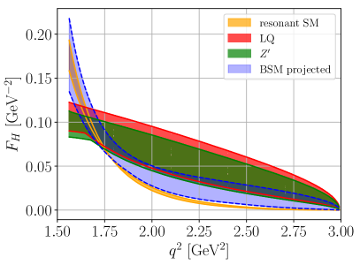
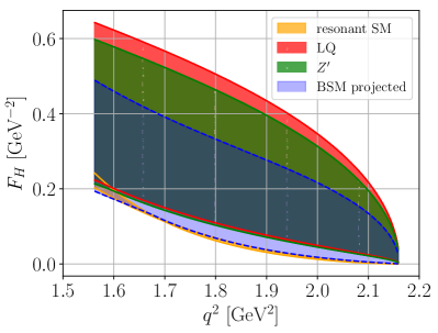
Note that scenarios with larger coupling $\lambda^{c\mu}_{S_{2}}\simeq 3.5$ Fajfer:2015mia ; Sahoo:2017lzi , that could induce significant $C_{S,P,T,T5}$ together with even a suppressed coupling to doublet quarks, are excluded by high-$p_{T}$ studies, $\lambda^{c\mu}_{S_{2}}\lesssim 0.4M_{S_{2}}/\mbox{TeV}$ Greljo:2017vvb . Taking this constraint into account leptoquark effects in $D\to\pi\mu^{+}\mu^{-}$ decays ($D_{s}\to K\mu^{+}\mu^{-}$ decays) in $A_{\rm FB}(q^{2})$ do not exceed (few) permille-level. On the other hand, $F_{H}(q^{2})\lesssim 0.1\,(\mbox{few}\times 0.1)$ for $D\to\pi\mu^{+}\mu^{-}$ decays ($D_{s}\to K\mu^{+}\mu^{-}$ decays) in the high $q^{2}$-region for $C^{\prime}_{9}=-C^{\prime}_{10}=0.63$ and small, however viable $C_{S}=C_{P}=11\,C_{T}=11\,C_{T5}=-0.0056$, with RG-factors between $C_{S,P}$ and $C_{T,T5}$ from Hiller:2016kry , see Fig. 8 (red bands). For the $Z^{\prime}$-model (green bands) with $C_{S,P,T,T5}=0$ but comparable maximal (axial-)vector contributions as the leptoquark one exhibits a similar small window for NP above the SM prediction (thin yellow band). The impact of the (pseudo-)scalar and tensor contributions on $F_{H}$ from viable leptoquark scenarios is thus very small.

It is apparent from Fig. 8 that the SM prediction of the angular observable $F_{H}$ (18) at high $q^{2}$ normalized to the high-$q^{2}$ integrated decay rate – unlike in Fig. 4, where the normalization is to the full decay rate – has very small theory uncertainties. The reason is that the high-$q^{2}$ region is dominated by a single resonance in $C_{9}^{R}$, the $\phi$, whose phase drops out in $F_{H}$. In the BSM curves the uncertainties, which are given by the band width, arise from interference with the SM, which prohibits the dropping of strong phases.

Leptoquark signals can hence be observed in $D\to P\ell\ell^{(\prime)}$ decays in lepton-universality tests, with corresponding effects from $C_{9,10}^{(\prime)}$ given in Tabs. 3 and 4, LFV searches and, if CP-violating, in $A_{\rm CP}$, illustrated in Fig. 6. LFV branching ratios from $S_{1,2}$ (cyan) together with SUSY predictions (brown, magenta) and in $Z^{\prime}$-models (green, blue) are shown in Fig. 9. There is a small window for NP signals from leptoquarks in the angular observable $F_{H}$ in the muon modes, shown in Fig. 8 by the red bands.

Figure 9: The differential branching ratio of $D^{+}\to\pi^{+}e^{\pm}\mu^{\mp}$ (plot to the left) and $D_{s}^{+}\to K^{+}e^{\pm}\mu^{\mp}$ (plot to the right) decays in models with leptoquarks $S_{1,2}$, $|K_{9}^{\prime}|=|K_{10}^{\prime}|=0.5$ (cyan), for two R-parity violating SUSY benchmarks, $K_{9}=-K_{10}=0.009$ (brown) and $K_{9}=-K_{10}=0.001$ (magenta), and in $Z^{\prime}$-model solution $2$, $K_{9}+K_{9}^{\prime}=-(K_{10}+K_{10}^{\prime})=4.6\times 10^{-3}$ (green), and solution $1$, $K_{9}+K_{9}^{\prime}=-(K_{10}+K_{10}^{\prime})=2.8\times 10^{-4}$ (blue). Solutions $3$-$6,8$ (not shown) give rates near the magenta RPV SUSY II band. See text for details.

IV.2 Charm reach of SUSY models

Supersymmetric SM extensions offer two ways for BSM signals in rare charm decays. One is through enhanced dipole couplings $C_{7}^{(\prime)}$ from scalar quark mixing; corresponding contributions to $c\to u\gamma$ decays have been studied recently in deBoer:2017que , to which we refer for details. The sensitivity of rare semileptonic $D\to P\ell^{+}\ell^{-}$ decays to $C_{7}^{(\prime)}$ can be read-off from Fig. 3 for the branching ratio and from Fig. 6 for the CP-asymmetry using Eq. (12). Note that the $D\to P\ell^{+}\ell^{-}$ distributions are sensitive to the sum of dipole coefficients, $C_{7}+C_{7}^{\prime}$, only. This ambiguity can be resolved with polarization studies in $D\to V\gamma$, $V=\rho,K^{*},\phi,K_{1}$ deBoer:2018zhz ; Adolph:2018hde , which probe the fraction of right-handed to left-handed photons. While the sensitivity window to NP in the branching ratio is rather small, there is large room in $A_{\rm CP}$ for CP-violating dipole contributions from supersymmetric flavor violation.

Another possibility to probe SUSY in $c\to u$ FCNCs is with R-parity violating terms $\lambda^{\prime}LQD$, which induce (axial)-vector couplings with $C_{9}=-C_{10}$ through tree level exchange of a scalar partner of a singlet down quark, see Burdman:2001tf for details; also Wang:2014uiz . However, this unavoidably involves doublet up-type quarks, hence is subject to constraints from rare kaon decays, specifically $K\to\pi\nu\bar{\nu}$. This situation resembles the one of the coupling to left-handed leptons of the scalar leptoquark $S_{1}$, which has the same quantum numbers as a singlet down quark. In SUSY additionally even stronger constraints from $K_{L}\to e^{\pm}\mu^{\mp}$ apply if the squark doublet masses are smaller or close to the down-singlet ones. We illustrate maximal LFV branching ratios in Fig. 9 for $K_{9}=-K_{10}\simeq 0.009$ (benchmark I) from $K\to\pi\nu\bar{\nu}$ Deandrea:2004ae for decoupled doublet squarks and $K_{9}=-K_{10}\simeq 0.001$ (benchmark II) from $K_{L}\to e^{\pm}\mu^{\mp}$ assuming degenerate squarks Allanach:1999ic ; Tanabashi:2018oca .

To summarize, the only realistic opportunity for SUSY to signal NP in $D\to P\ell^{+}\ell^{-}$ decays is with CP-violating contributions in $A_{\rm CP}$, illustrated in Fig. 6, and in LFV branching ratios in R-parity violating models, shown in Fig. 9.

IV.3 Flavorful $Z^{\prime}$–models

The effective $Z^{\prime}$–interaction Hamiltonian part for $c\to u\ell^{-}\ell^{\prime+}$ processes can be written as

$$\mathcal{H}_{Z^{\prime}}\supset\left(g_{L}^{uc}\,\overline{u}_{L}\gamma_{\mu}c_{L}+g_{R}^{uc}\,\overline{u}_{R}\gamma_{\mu}c_{R}+g_{L}^{\ell\ell^{\prime}}\,\overline{\ell}_{L}\gamma_{\mu}\ell_{L}^{\prime}+g_{R}^{\ell\ell^{\prime}}\,\overline{\ell}_{R}\gamma_{\mu}\ell_{R}^{\prime}\right)Z^{\prime\,\mu}+{\rm h.c.}\,.$$ (34)

The following Wilson coefficients are induced at tree-level

$$C_{9/10}^{(\ell\ell)} =-{\pi\over\sqrt{2}G_{F}\alpha_{e}}\,{g_{L}^{uc}\bigl{(}g_{R}^{\ell\ell}\pm g_{L}^{\ell\ell}\bigr{)}\over M_{Z^{\prime}}^{2}}\,,\quad C_{9/10}^{\prime\,(\ell\ell)}=-{\pi\over\sqrt{2}G_{F}\alpha_{e}}\,{g_{R}^{uc}\bigl{(}g_{R}^{\ell\ell}\pm g_{L}^{\ell\ell}\bigr{)}\over M_{Z^{\prime}}^{2}}\,,$$ (35)

$$K_{9/10}^{(\ell\ell^{\prime})} =-{\pi\over\sqrt{2}G_{F}\alpha_{e}}\,{g_{L}^{uc}\bigl{(}g_{R}^{\ell\ell^{\prime}}\pm g_{L}^{\ell\ell^{\prime}}\bigr{)}\over M_{Z^{\prime}}^{2}}\,,\quad K_{9/10}^{\prime\,(\ell\ell^{\prime})}=-{\pi\over\sqrt{2}G_{F}\alpha_{e}}\,{g_{R}^{uc}\bigl{(}g_{R}^{\ell\ell^{\prime}}\pm g_{L}^{\ell\ell^{\prime}}\bigr{)}\over M_{Z^{\prime}}^{2}}\,.$$ (36)

Using Eqs. (13),(26) and (11), respectively, we obtain the following constraints on the $Z^{\prime}$–model

$$\bigl{|}(g_{L}^{uc}-g_{R}^{uc})(g_{L}^{\mu\mu}-g_{R}^{\mu\mu})\big{|}\lesssim 0.03\,\left({M_{Z^{\prime}}\over 1~{}{\rm TeV}}\right)^{2}\,,$$

$$\bigl{|}g_{L}^{uc}-g_{R}^{uc}\bigr{|}\sqrt{\bigl{|}g_{L}^{\mu e}\bigr{|}^{2}+\bigl{|}g_{R}^{\mu e}\bigr{|}^{2}}\lesssim 0.07\,\left({M_{Z^{\prime}}\over 1~{}{\rm TeV}}\right)^{2}\,,$$ (37)

$$\bigl{|}g_{L}^{uc}+g_{R}^{uc}\bigr{|}\,\sqrt{\bigl{|}g_{L}^{\mu\mu}\bigr{|}^{2}+\bigl{|}g_{R}^{\mu\mu}\bigr{|}^{2}}\lesssim 0.04\,\left({M_{Z^{\prime}}\over 1~{}{\rm TeV}}\right)^{2}\,,$$

where $M_{Z^{\prime}}$ denotes the mass of the $Z^{\prime}$. Stronger bounds, however, arise from the $Z^{\prime}$ tree level contribution to $D^{0}-\overline{D}^{0}$ mixing, see App. B for details (Here and in the following the superscript ’$uc$’ has been dropped.),

$$g_{L}^{2}+g_{R}^{2}-X\,g_{L}\,g_{R}\simeq(4.2\pm 1.5)\times 10^{-7}\,\left({M_{Z^{\prime}}\over 1~{}{\rm TeV}}\right)^{2}\,,$$ (38)

with $X\sim 20$ for $1\,{\rm TeV}\lesssim M_{Z^{\prime}}\lesssim 10\,{\rm TeV}$. Main uncertainties are due to the experimental limit on the $D^{0}-\overline{D}^{0}$ mixing parameter and the hadronic matrix elements. In the case of only one non-zero coupling present ($g_{L}\neq 0$ and $g_{R}=0$ or $g_{R}\neq 0$ and $g_{L}=0$), constraints are severe, $|g_{L/R}|\lesssim 8\times 10^{-4}\,(M_{Z^{\prime}}/{\rm TeV})$; assuming order one muon couplings in Eq. (37), the resulting bounds on the BSM Wilson coefficients read $C_{9/10}\lesssim\mathcal{O}(10^{-2})$ for $M_{Z^{\prime}}\gtrsim 1\,$TeV, consistent with Fajfer:2015mia . However, the presence of both couplings $g_{L}\neq 0$ and $g_{R}\neq 0$ allows to satisfy the mixing constraints even with arbitrarily large values, bounded only by Eq. (37), see App. B for details, if

$$g_{L}\approx Xg_{R}\quad\text{or}\quad g_{L}\approx\frac{1}{X}g_{R}\,.$$ (39)

In the following we show that these conditions can be met in flavorful $Z^{\prime}$–models by flavor rotations without introducing unnatural hierarchies. Here, FCNC $c\to u$–transitions arise from non-universal charges, denoted by $F$. Specifically, inducing $g_{L}$ ($g_{R}$) requires the charges of the doublet (singlet) charm and up-quarks to be different from each other

$$\Delta F_{L}=F_{Q_{2}}-F_{Q_{1}}\,,\quad\Delta F_{R}=F_{u_{2}}-F_{u_{1}}\,,$$ (40)

i.e., $\Delta F_{L(R)}\neq 0$. Another requisite ingredient is flavor mixing. Four such rotations between flavor and mass bases exist, those for up-singlets, $U_{u}$, for down-singlets $U_{d}$, and those for up- and down-doublets, $V_{u}$ and $V_{d}$, respectively. $U_{d},U_{u},V_{u}$ and $V_{d}$ are unitary matrices; in absence of a theory of flavor they are unconstrained, except for $V_{u}^{\dagger}V_{d}=V_{\rm CKM}$. Here we consider rotations residing in the up-sector, $U_{d}=1,V_{d}=1$, hence $V_{u}=V_{\rm CKM}^{\dagger}$, as flavor rotations in the down sector are subject to strong constraints from the rare kaon decays, e.g. Buras:2012jb . Small mixings, $(V_{d})_{12}/(V_{u})_{12}\lesssim 10^{-3}$, however, would still be consistent with sizable effects in charm. To understand the interplay between rotations and charges in order to satisfy Eq. (39), we simplify the analysis by assuming the third generations to be sufficiently decoupled. This allows us to work with 2 by 2 orthogonal matrices, parametrized by a single angle each, $\theta_{u}$ and $\Phi_{u}$ for the up-singlets and -doublets, respectively. Then,

$$g_{L}=g_{4}\,\Delta F_{L}\cos\Phi_{u}\sin\Phi_{u}\,,\quad g_{R}=g_{4}\,\Delta F_{R}\cos\theta_{u}\sin\theta_{u}\,,$$ (41)

with $g_{4}$ the $U(1)^{\prime}$ gauge coupling strength and, since $V_{u}=V_{\rm CKM}^{\dagger}$, we obtain

$$\frac{g_{R}}{g_{L}}\simeq\frac{\Delta F_{R}\cos\theta_{u}\sin\theta_{u}}{\Delta F_{L}\lambda}\,,$$ (42)

where $\lambda\sim 0.2$ denotes the Wolfenstein parameter.

We obtain $g_{R}/g_{L}=X$ for

$$\frac{\Delta F_{R}}{\Delta F_{L}}\sin 2\theta_{u}\simeq 8\,,$$ (43)

and $g_{R}/g_{L}=1/X$ for

$$\frac{\Delta F_{R}}{\Delta F_{L}}\sin\theta_{u}\simeq 1/100\,.$$ (44)

The former case, in the following termed right-handed (RH)-dominated, requires some mild hierarchy between the left versus right charges, whereas the latter case, termed left-handed (LH)-dominated, can be accommodated with mixing alone $\theta_{u}\sim 10^{-2}$. In either case, the ratio of left- and right-handed couplings is fixed,

$$\frac{C_{9/10}}{C_{9/10}^{\prime}},\frac{K^{(\ell\ell^{\prime})}_{9/10}}{K^{(\prime)\,(\ell\ell^{\prime})}_{9/10}}\sim X~{}(\mbox{LH})~{}~{}\mbox{or}~{}~{}\sim 1/X~{}(\mbox{RH})\,.$$ (45)

In Tab. 5 we present sample scenarios of $Z^{\prime}$–models with sizable BSM coefficients, which obey Eq. (39). The models differ in their charge assignments, all of which fulfill anomaly cancellation conditions, see App. C for details. For the models presented $\Delta F_{R}/\Delta F_{L}$ ranges within $\sim[0.9,\,35]$. Also given are the values of the mixing angle $\theta_{u}$ for each model. Models with $\Delta F_{R}/\Delta F_{L}\geq 8$ can be either RH or LH-dominated, depending on the flavor rotation $\theta_{u}$.

Table 5: Scenarios of anomaly-free $Z^{\prime}$–models and the mixing angle $\theta_{u}$ for different charge assignments taken from Tab. 6. The primed solutions are RH-dominated, whereas the unprimed ones are LH-dominated.

sol. $\#$	$\Delta F_{R}$		$\Delta F_{L}$		$g_{R}/g_{L}$ case		$\theta_{u}$
1	3		2		$1/X$		0.008
2	12		9		$1/X$		0.009
$3^{\prime}$	35		1		$X$		0.122
3	35		1		$1/X$		0.0003
4	3		3		$1/X$		0.011
5	3		3		$1/X$		0.011
6	15		16		$1/X$		0.012
7	0		0		-		-
$8^{\prime}$	18		1		$X$		0.244
8	18		1		$1/X$		0.0006

We work out constraints on the parameters of the concrete $Z^{\prime}$–models. The constraints from $D\to\pi\mu^{+}\mu^{-}$ branching ratios in Eq. (11), using $g_{L}^{\ell\ell}=g_{4}F_{L_{\ell}},\,g_{R}^{\ell\ell}=g_{4}F_{e_{\ell}}$, can be written as

$$g_{4}^{4}\left(\lambda\,\Delta F_{L}\right)^{2}\left\{1+\left(\frac{\Delta F_{R}\sin 2\theta_{u}}{\Delta F_{L}2\lambda}\right)\right\}^{2}\left(F_{L_{2}}^{2}+F_{e_{2}}^{2}\right)\lesssim 1.8\times 10^{-3}\,\,\left({M_{Z^{\prime}}\over 1~{}{\rm TeV}}\right)^{4}\,.$$ (46)

Imposing in addition the constraints from $D^{0}-\overline{D}^{0}$ mixing fixes $g_{4}/M_{Z^{\prime}}$ for each model, with two solutions for those with large $\Delta F_{R}/\Delta F_{L}$. We obtain

$$g_{4}^{2}\lesssim\frac{0.21}{\Delta F_{L}\,\sqrt{F_{L_{2}}^{2}+F_{e_{2}}^{2}}}\,\left(\frac{M_{Z^{\prime}}}{1\,\text{TeV}}\right)^{2}\times\begin{cases}(1+X)^{-1}~{}~{}(\mbox{RH})\\ (1+1/X)^{-1}~{}~{}(\mbox{LH})\end{cases}\quad.$$ (47)

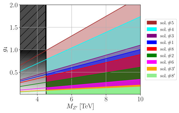
In Fig. 10 the BSM coupling $g_{4}$ is shown as a function of the $Z^{\prime}$ mass. Each line corresponds to an upper limit in the scenarios from Tab. 5 with one specific choice for the charges $F_{L_{1}}\,(F_{L_{2}})$ and $F_{e_{1}}\,(F_{e_{2}})$ for electrons (muons). Constraints for RH cases are stronger than for corresponding LH ones in Eq. (47). The black region shows the exclusion region due to resonance searches in dilepton searches of $M_{Z^{\prime}}>4.5\,$TeV Tanabashi:2018oca . The true lower bound for the $Z^{\prime}$ mass is different for every solution due to the different quark charge assignments and overall coupling strength and in general different for electrons and muons. Therefore, part of the region $g_{4}<0.5$ and $M_{Z^{\prime}}<4.5\,$TeV might still be viable or constrained by other searches Smolkovic:2019jow .

Figure 10: Upper limits on the $U(1)^{\prime}$ gauge coupling $g_{4}$ as a function of the $Z^{\prime}$ mass (47) for the models in Tab. 5. The black region is excluded by direct searches in dimuon and dielectron spectra Tanabashi:2018oca . For lower values of $g_{4}$, the bounds become model-dependent as indicated by the lighter color, see main text.

$Z^{\prime}$-contributions to charged LFV arise by a similar misalignment between flavor and mass bases as for the quarks. Likewise, there is no left-handed charged LFV if the PMNS-matrix is only due to rotations in the neutrino sector. In the presence of charged lepton rotations, the decays $(i)$ $\tau\to(\mu,e)\ell\ell$ with $\ell=e,\mu$ , as well as $(ii)$ $\mu\to eee$ and $\mu\to e\gamma$ provide the most stringent constraints Tanabashi:2018oca . Charm constraints, shown in Fig. 10, continue to be more restrictive for the scenarios in Tab. 5 if the charged lepton rotations are ${\cal{O}}(10^{-2}$–$10^{-3})$ and ${\cal{O}}(10^{-4}$–$10^{-5})$ or smaller for the modes $(i)$ and $(ii)$, respectively. Upper limits on $D\to\pi e^{\pm}\mu^{\mp}$ and $D_{s}\to Ke^{\pm}\mu^{\mp}$ branching ratios consistent with leptonic LFV data are shown in Fig. 9.

As we work in the limit $V_{u}=V_{\text{CKM}}^{\dagger}$ we automatically avoid $Z^{\prime}$-FCNCs with down-type doublet quarks and hence are unable to address present discrepancies in semileptonic rare $B$-decays between the data and the SM. We would like to point out, however, that simultaneous left-handed contributions to $|\Delta c|=|\Delta u|=1$ and $|\Delta b|=|\Delta s|=1$ arise if $V_{us}$ stems from up-rotations and $V_{cb}$ from down-rotations. A detailed investigation is beyond the scope of this work.

To summarize, flavorful $Z^{\prime}$-models can signal NP in lepton-universality tests, with corresponding effects from $C_{9,10}^{(\prime)}$ given in Tabs. 3 and 4. As we neglect in the $U(1)^{\prime}$-study CP-phases in the flavor rotations there are no CP-asymmetries. We illustrate maximal effects in $F_{H}$ in the muon modes in Fig. 8 for $C_{9}+C_{9}^{\prime}=-(C_{10}+C_{10}^{\prime})=0.63$ (green bands), leaving a small window above the SM at high $q^{2}$. Charged LFV effects in $Z^{\prime}$-models are model-dependent, with branching ratios $\mathcal{B}\left(D\to\pi\mu^{\pm}e^{\mp}\right)\lesssim\text{few}\,10^{-12}$ and $\mathcal{B}\left(D_{s}\to K\mu^{\pm}e^{\mp}\right)\lesssim 10^{-12}$, see Fig. 9.

V Conclusions

We worked out the NP sensitivity of $|\Delta c|=|\Delta u|=1$ SM null tests based on lepton-universality in Sec. III.2, angular distributions in Sec. III.3, approximate CP–symmetry in Sec. III.4 and lepton flavor conservation in Sec. III.5 in $D\to\pi\ell\ell^{(\prime)}$ and $D_{s}\to K\ell\ell^{(\prime)}$ decays into electrons or muons. These studies provide a rich arena to test the SM and look for different kinds of BSM phenomena:

For $q^{2}$–values above the $\phi$, a region with lesser resonance pollution, see Fig. 2, branching ratios are about $\mathcal{O}(10^{-9}$–$10^{-8})$. Here, lepton universality tests $R_{\pi}^{D}$ and $R_{K}^{D_{s}}$ can be sizable, up to ${\mathcal{O}}(10)$, and cleanly signal BSM physics which exhibits more differences between electrons and muons than their mass, see Tabs. 3 and 4. The angular observables $A_{\rm FB}$ and $F_{H}$ and CP–asymmetries, the latter around the $\phi$ as well, can be of the order one, see Figs. 5 and 6. Due to the somewhat smaller $q^{2}$–integrated decay rates, which appear in the null test observables $F_{H},A_{\rm FB}$ and $A_{\rm CP}$ in the denominator, NP effects in $D_{s}\to K\ell^{+}\ell^{-}$ decays are pronounced relative to the ones in $D\to\pi\ell^{+}\ell^{-}$. Semileptonic LFV branching ratios can reach $\mathcal{O}(10^{-7})$ model-independently, see Fig. 7.

Concrete models with potentially large (pseudo)scalar and tensor contributions, which could be signaled with angular observables, are scalar leptoquarks with representations $S_{1}$ and $S_{2}$. However, it is exactly those representations that allow for chirality flipping operators that are unavoidably subject to tight constraints from the kaon sector. The largest effects in charm decays within leptoquark models are therefore from couplings to right-handed up-quarks, inducing primed (axial-)vector operators. Both right-handed and left-handed (axial-)vector couplings $C_{9,10}^{(\prime)}$ are generically induced in $Z^{\prime}$–models. We give explicit examples with generation-dependent $U(1)^{\prime}$-charges that are anomaly-free (App. C).

Sizable BSM (axial-)vector couplings, as in leptoquarks $S_{1,2},\widetilde{V}_{1,2}$ and flavorful $U(1)^{\prime}$-models, can be probed in all null test observables analyzed in this work, except for $A_{\rm FB}$. There is a small window for NP in $F_{H}$ in the muon modes at high $q^{2}$, shown in Fig. 8. SUSY models with flavor mixing are prime suspects for chirally-enhanced dipole contributions. CP-violating BSM dipole operators in semileptonic modes can be probed with $A_{\rm CP}$. The sensitivity to the dipole operators is similar to the one of the four-fermion ones since both types appear in the combination (12), which contains the sum of $C_{7}$ and $C_{7}^{\prime}$. Polarization studies in $D\to V\gamma$, $V=\rho,K^{*},\phi,K_{1}$ deBoer:2018zhz ; Adolph:2018hde , on the other hand, are sensitive to the fraction of right-handed to left-handed photons. R-parity violating SUSY LFV branching ratios can reach $\mathcal{O}(10^{-11})$, see Fig. 9. Each BSM model’s section, Sec. IV.1 (leptoquarks), Sec. IV.2 (SUSY) and Sec. IV.3 (flavorful $Z^{\prime}$-models) ends with a brief summary of possible "smoking gun"-observables for new physics.

The analysis in $U(1)^{\prime}$–models explicitly highlights the complementarity between charm and $K$ and $B$–physics. Tree level $Z^{\prime}$–induced FCNCs arise only if the quark flavor basis is sufficiently misaligned with the up quark mass basis, and CKM stems predominantly from up-rotations. Looking for BSM physics in charm can therefore provide unique insights into the origin of flavor structure of fundamental matter.

Appendix A Form Factors

The hadronic matrix elements for $D\to P$ transitions are parametrized in terms of three form factors, $f_{+\,,0\,,T}(q^{2})$, defined as 

$$\langle P(k)|\bar{u}\gamma^{\mu}c|D(p)\rangle=\left[(p+k)^{\mu}-{m_{D}^{2}-m_{P}^{2}\over q^{2}}q^{\mu}\right]f_{+}(q^{2})+q^{\mu}{m_{D}^{2}-m_{P}^{2}\over q^{2}}f_{0}(q^{2})\,,$$ (48)

$$\langle P(k)|\bar{u}\sigma^{\mu\nu}(1\pm\gamma_{5})c|D(p)\rangle=-\text{i}\,(p^{\mu}k^{\nu}-k^{\mu}p^{\nu}\pm\text{i}\,\epsilon^{\mu\nu\rho\sigma}p_{\rho}k_{\sigma}){2f_{T}(q^{2})\over m_{D}+m_{P}}\,.$$ (49)

In this work we use the $D\to\pi$ form factors computed recently by Lubicz et al. Lubicz:2017syv ; Lubicz:2018rfs using lattice QCD (LQCD), parametrized in terms of the $z$–expansion as, $i=+,0,T$,

$$f_{i}(q^{2})={1\over 1-P_{i}\,q^{2}}\biggl{[}f_{i}(0)+c_{i}\,(z(q^{2})-z(0))\,\biggl{(}1+{z(q^{2})+z(0)\over 2}\biggr{)}\biggr{]}\,,$$ (50)

where

$$z(q^{2})={\sqrt{t_{+}-q^{2}}-\sqrt{t_{+}-t_{0}}\over\sqrt{t_{+}-q^{2}}+\sqrt{t_{+}-t_{0}}}\,,\quad t_{\pm}=(m_{D}\pm m_{P})^{2}\,,\quad t_{0}=(m_{D}+m_{P})(\sqrt{m_{D}}-\sqrt{m_{P}})^{2}\,.$$ (51)

The numerical values of $f_{i}(0)$, $c_{i}$ and $P_{i}$ parameters together with their uncertainties and covariance matrices are given in Lubicz:2017syv ; Lubicz:2018rfs  . In particular, $P_{0,\,T}$ and $c_{T}$ have large uncertainties, about 40% and 90%, respectively, such that naïve variation of parameters independently produces larger(huge) uncertainties for $f_{+,0}$($f_{T}$) at high $q^{2}$. Taking into account correlations, we present in Fig. 11 the $D\to\pi$ form factors within $1\sigma$ uncertainties.

Figure 11: The $D\to\pi$ form factors $f_{+},f_{0},f_{T}$ from lattice QCD Lubicz:2017syv ; Lubicz:2018rfs and $f_{+}$ from HFLAV Amhis:2016xyh (gray band) with $1\sigma$ theoretical uncertainties.

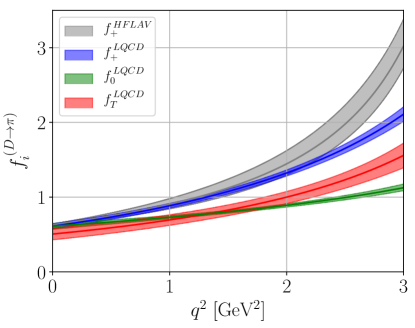
Also shown (gray band) is $f_{+}$ obtained from the HFLAV collaboration Amhis:2016xyh , parametrized as

$$f_{+}(q^{2})={1\over\phi(q^{2})}\sum_{k=0}^{2}a_{k}\,z^{k}(q^{2})\,,$$ (52)

where the parameters $r_{k}=a_{k}/a_{0}$ are extracted from data on semileptonic $D\to\pi\ell\overline{\nu}$ decays from several experiments. Both results for $f_{+}$ are in good agreement with each other up to $q^{2}\gtrsim 2.3\,\mbox{GeV}^{2}$. Towards the low recoil end point, $f_{+}^{\rm HFLAV}/f_{+}^{\rm LQCD}\simeq 1.4$ at $q_{\rm max}^{2}=(m_{D}-m_{\pi})^{2}$. Symmetry breaking effects in the form factor relation $f_{T}=f_{+}(1+\mathcal{O}(\alpha_{s},\Lambda_{\rm QCD}/m_{c}))$ amount to about ${\cal{O}}(30\%)$ in the LQCD results. We assume the $D_{s}\to K$ and $D\to\pi$ form factors to be the same, supported by the lattice study Koponen:2012di . The $D^{0}\to\pi^{0}$ form factors receive an additional isospin factor $f_{i}\to f_{i}/\sqrt{2}$.

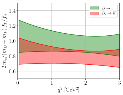
In Fig. 12 we show the factor $\gamma=\frac{2m_{c}}{m_{D}+m_{P}}\frac{f_{T}}{f_{+}}$, defined in Eq. (12) for the $D\to\pi$ ($D_{s}\to K$) transition in green (red). As noted previously, $\gamma\approx 1$ is a good approximation in the full $q^{2}$–range.

Figure 12: The $q^{2}$–dependence of the factor $\gamma=\frac{2m_{c}}{m_{D}+m_{P}}\frac{f_{T}}{f_{+}}$, defined in Eq. (12) for $D\to\pi$ (green) and $D_{s}\to K$ (red).

Appendix B Constraints from $D^{0}-\overline{D}^{0}$ mixing

We compute constraints from the current world average of the $D^{0}-\overline{D}^{0}$ mixing parameter $x_{D}$ Amhis:2016xyh

$$x_{D}^{\text{exp}}=(4.1^{+1.4}_{-1.5})\times 10^{-3}\,,$$ (53)

defined as

$$\begin{split}x_{D}=\frac{\Delta m_{D^{0}}}{\Gamma_{D^{0}}}=\frac{2\,|M_{12}|}{\Gamma_{D^{0}}}=\frac{2}{\Gamma_{D^{0}}}\,\frac{1}{2m_{D^{0}}}\,\langle D^{0}|\mathcal{H}_{\rm eff}^{\Delta c=2}|\overline{D}^{0}\rangle\,.\end{split}$$ (54)

Here, $\mathcal{H}^{\Delta c=2}_{\rm eff}=\sum_{i}c_{i}Q_{i}$ and Golowich:2009ii

$$\begin{split}Q_{1}&=(\overline{u}_{L}\gamma_{\mu}c_{L})(\overline{u}_{L}\gamma^{\mu}c_{L})\,,\quad Q_{5}=(\overline{u}_{R}\sigma_{\mu\nu}c_{L})(\overline{u}_{R}\sigma^{\mu\nu}c_{L})\,,\\ Q_{2}&=(\overline{u}_{L}\gamma_{\mu}c_{L})(\overline{u}_{R}\gamma^{\mu}c_{R})\,,\quad Q_{6}=(\overline{u}_{R}\gamma_{\mu}c_{R})(\overline{u}_{R}\gamma^{\mu}c_{R})\,,\\ Q_{3}&=(\overline{u}_{L}c_{R})(\overline{u}_{R}c_{L})\,,\quad\quad\quad\,Q_{7}=(\overline{u}_{L}c_{R})(\overline{u}_{L}c_{R})\,,\\ Q_{4}&=(\overline{u}_{R}c_{L})(\overline{u}_{R}c_{L})\,,\quad\quad\quad\,Q_{8}=(\overline{u}_{L}\sigma_{\mu\nu}c_{R})(\overline{u}_{L}\sigma^{\mu\nu}c_{R})\,.\end{split}$$ (55)

In the $Z^{\prime}$–model the following $\Delta C=2$ Wilson coefficients are induced at the scale $\mu=M_{Z^{\prime}}$

$$c_{1}(M_{Z^{\prime}}) =\frac{g_{L}^{2}}{2M_{Z^{\prime}}^{2}}\,,~{}c_{2}(M_{Z^{\prime}})=\frac{g_{L}\,g_{R}}{M_{Z^{\prime}}^{2}}\,,~{}c_{6}(M_{Z^{\prime}})=\frac{g_{R}^{2}}{2M_{Z^{\prime}}^{2}}\,.$$ (56)

The operator $Q_{3}$ is radiatively induced and needs to be taken into account as well. At the scale $\mu=3$ GeV the $Z^{\prime}$–contribution is given as Golowich:2007ka ; Golowich:2009ii

$$\begin{split}x_{D}^{Z^{\prime}}=\frac{1}{\Gamma_{D^{0}}m_{D^{0}}}\,&\left[\phantom{\frac{1}{2}}r_{1}\,c_{1}(M_{Z^{\prime}})\,\langle Q_{1}\rangle+\sqrt{r_{1}}\,c_{2}(M_{Z^{\prime}})\,\langle Q_{2}\rangle\right.\\ &\left.+\,\frac{2}{3}\,c_{2}(M_{Z^{\prime}})\,(\sqrt{r_{1}}-r_{1}^{-4})\,\langle Q_{3}\rangle+r_{1}\,c_{6}(M_{Z^{\prime}})\,\langle Q_{6}\rangle\phantom{\frac{1}{2}}\right]\,,\end{split}$$ (57)

with the renormalization factor

$$r_{1}=\left(\frac{\alpha_{s}(M_{Z^{\prime}})}{\alpha_{s}(m_{t})}\right)^{2/7}\left(\frac{\alpha_{s}(m_{t})}{\alpha_{s}(m_{b})}\right)^{6/23}\left(\frac{\alpha_{s}(m_{b})}{\alpha_{s}(\mu)}\right)^{6/25}\,,$$ (58)

and the hadronic matrix elements computed at $\mu=3\,$GeV Bazavov:2017weg

$$\begin{split}\langle Q_{1}\rangle&=\phantom{-}0.0805(55)=\langle Q_{6}\rangle\,,\\ \langle Q_{2}\rangle&=-0.2070(142)\,,\\ \langle Q_{3}\rangle&=\phantom{-}0.2747(129)\,.\end{split}$$ (59)

In terms of the $Z^{\prime}$–model parameters one obtains from Eq. (57)

$$x_{D}^{Z^{\prime}}=\frac{r_{1}\langle Q_{1}\rangle}{2\,\Gamma_{D^{0}}\,m_{D^{0}}}\,\frac{g_{L}^{2}+g_{R}^{2}-Xg_{L}g_{R}}{M_{Z^{\prime}}^{2}}\,,$$ (60)

where

$$X =-2\,\left(\sqrt{r_{1}}\,\langle Q_{2}\rangle+\,\frac{2}{3}\,(\sqrt{r_{1}}-r_{1}^{-4})\,\langle Q_{3}\rangle\right)\left(r_{1}\langle Q_{1}\rangle\right)^{-1}\,,$$ (61)

and recovers Eq. (38). Numerically, $X=19.2,\,24.0,\,26.2$ for $M_{Z^{\prime}}=1,5,10$ TeV, respectively. To obtain the approximations (39), we rewrite Eq. (38) as

$$|g_{L}|=|g_{R}|\,\left(\frac{X}{2}\pm\,\sqrt{\left(\frac{X^{2}}{4}-1\right)+\frac{\tilde{x}}{|g_{R}|^{2}}}\right)\,,\quad\tilde{x}=\frac{2\,x_{D}^{\text{exp}}\,\Gamma_{D^{0}}\,m_{D^{0}}\,M^{2}_{Z^{\prime}}}{r_{1}\langle Q_{1}\rangle}\,,$$ (62)

and employ $\tilde{x}\ll|g_{R}|^{2}$ and $4/X^{2}\ll 1$.

Experimental constraints on CP-violation in $D^{0}-\overline{D}^{0}$ mixing, $x_{12}\sin\phi_{12}\lesssim 2\times 10^{-4}$, are stronger than (53) by about $\sim 0.04$ Amhis:2016xyh ; Gedalia:2009kh . Both SUSY and leptoquark models contribute to $\Delta C=2$ Wilson coefficients with the square of the couplings relevant for $\Delta C=1$ coefficients. For instance, $C_{7}^{(\prime)}$ in SUSY is proportional to one power of flavor-violating scalar quark mass terms whereas mixing is induced at second order. Constraints on the $\Delta C=1$ couplings from mixing allowing for order one phases are hence about $\sim 0.2$ stronger than without CP-phases.

Appendix C Anomaly-free $Z^{\prime}$–models

We consider $Z^{\prime}$–extensions of the SM with generation-dependent $U(1)^{\prime}$–charges $F_{\psi_{i}}$ for quarks and leptons $\psi=Q,u,d,L,e,\nu$ in representations under $SU(3)_{C}\times SU(2)_{L}\times U(1)_{Y}\times U(1)^{\prime}$

$$\begin{split}Q_{i}&\sim(3,2,1/6,F_{Q_{i}})\,,\quad u_{i}\sim(3,1,2/3,F_{u_{i}})\,,\quad d_{i}\sim(3,1,-1/3,F_{d_{i}})\,,\\ L_{i}&\sim(1,2,-1/2,F_{L_{i}})\,,\quad e_{i}\sim(1,1,-1,F_{e_{i}})\,,\quad\nu_{i}\sim(1,1,0,F_{\nu_{i}})\,,\end{split}$$ (63)

where we allow for the possibility of having three RH neutrinos $\nu$. The charges $F_{\psi_{i}}$ are subject to constraints from gauge anomaly cancellation conditions (ACCs). An excellent introduction to the subject is given in Bilal:2008qx , for recent phenomenological applications, see, for instance, Ellis:2017nrp ; Allanach:2018vjg ; Rathsman:2019wyk ; Costa:2019zzy . The ACCs read Allanach:2018vjg :

$$SU(3)_{C}^{2}\times U(1)_{F}^{\prime}:\quad\quad \sum_{i=1}^{3}\,\left(2F_{Q_{i}}-F_{u_{i}}-F_{d_{i}}\right)=0\,,$$ (64)

$$SU(2)_{L}^{2}\times U(1)_{F}^{\prime}:\quad\quad \sum_{i=1}^{3}\,\left(3F_{Q_{i}}+F_{L_{i}}\right)=0\,,$$ (65)

$$U(1)_{Y}^{2}\times U(1)_{F}^{\prime}:\quad\quad \sum_{i=1}^{3}\,\left(F_{Q_{i}}+3F_{L_{i}}-8F_{u_{i}}-2F_{d_{i}}-6F_{e_{i}}\right)=0\,,$$ (66)

gauge-gravity: $$\sum_{i=1}^{3}\,\left(6F_{Q_{i}}+2F_{L_{i}}-3F_{u_{i}}-3F_{d_{i}}-F_{e_{i}}-F_{\nu_{i}}\right)=0\,,$$ (67)

$$U(1)_{Y}\times U(1)^{\prime 2}_{F}:\quad\quad \sum_{i=1}^{3}\,\left(F^{2}_{Q_{i}}-F^{2}_{L_{i}}-2F^{2}_{u_{i}}+F^{2}_{d_{i}}+F^{2}_{e_{i}}\right)=0\,,$$ (68)

$$U(1)_{F}^{\prime 3}:\quad\quad \sum_{i=1}^{3}\,\left(6F^{3}_{Q_{i}}+2F^{3}_{L_{i}}-3F^{3}_{u_{i}}-3F^{3}_{d_{i}}-F^{3}_{e_{i}}-F^{3}_{\nu_{i}}\right)=0\,.$$ (69)

Since they are SM singlets, the RH neutrinos only appear in Eqs. (67),(69). In the SM+$3\nu_{R}$ (the SM), the 18 (15) charges are constrained by 6 ACCs. Important features of the ACCs and their solutions are (see Allanach:2018vjg and references therein for details):

• Rational solutions: We assume that all $U(1)^{\prime}$–charges are rational numbers $F_{\psi}\in\mathbb{Q}$ .

• Rescaling invariance: Any solution of the ACCs can be rescaled by any rational number $k\in\mathbb{Q}$ , $F_{\psi}\rightarrow kF_{\psi},\,\forall\psi\in\left\{Q_{i},u_{i},d_{i},L_{i},e_{i},\nu_{i}\right\}$, which constitutes another solution. As rescaling all charges is equivalent to a rescaling of the $U(1)^{\prime}$ gauge coupling, these solutions are in the same equivalence class and, hence, are not independent from each other. We therefore assume integer solutions $F_{\psi}\in\mathbb{Z}$ without loss of generality.

• Permutation invariance of fermions: The ACCs are invariant under the permutation of generation indices within each specific species $\psi$.

To extract concrete solutions of the non-linear Eqs. (64)-(69), we use computational algebraic geometry and perform a Gröbner basis computation Rathsman:2019wyk with the aid of Mathematica and obtain analytical expressions for the charges $F_{\psi}$. We impose phenomenological constraints, for instance, $F_{d_{i}}=F_{\nu_{i}}=0$, to further reduce the number of free parameters. We then search for integer charges for all fermions by employing rescaling invariance, and focus on solutions with the smallest absolute value of the sum of all charges. To obtain large $c\to u$ FCNCs we search for solutions with $\Delta F_{L,R}\neq 0$, see Eq. (40), that are consistent with Eq. (43).

Table 6: Sample solutions of the ACCs (64)-(69) in a $U(1)^{\prime}$ extension of the SM$+3\nu_{R}$. Only solutions 4, 7 require RH neutrinos. The ordering of generations is arbitrary due to permutation invariance, see text.

solution $\#$	$F_{Q_{i}}$	$F_{u_{i}}$	$F_{d_{i}}$	$F_{L_{i}}$	$F_{e_{i}}$	$F_{\nu_{i}}$
1	$\begin{matrix}-4&-2&\phantom{-}6\\ \end{matrix}$	$\begin{matrix}-2&\phantom{-}1&\phantom{-}1\\ \end{matrix}$	$\begin{matrix}\phantom{-}0&\phantom{-}0&\phantom{-}0\\ \end{matrix}$	$\begin{matrix}-8&\phantom{-}3&\phantom{-}5\\ \end{matrix}$	$\begin{matrix}-3&-3&\phantom{-}6\\ \end{matrix}$	$\begin{matrix}\phantom{-}0&\phantom{-}0&\phantom{-}0\\ \end{matrix}$
2	$\begin{matrix}-6&\phantom{-}3&\phantom{-}3\\ \end{matrix}$	$\begin{matrix}-8&\phantom{-}4&\phantom{-}4\\ \end{matrix}$	$\begin{matrix}-10&\phantom{-}0&\phantom{-}10\\ \end{matrix}$	$\begin{matrix}-6&\phantom{-}1&\phantom{-}5\\ \end{matrix}$	$\begin{matrix}\phantom{-}0&\phantom{-}0&\phantom{-}0\\ \end{matrix}$	$\begin{matrix}\phantom{-}0&\phantom{-}0&\phantom{-}0\\ \end{matrix}$
3	$\begin{matrix}-20&\phantom{-}7&\phantom{-}8\\ \end{matrix}$	$\begin{matrix}-29&\phantom{-}3&\phantom{-}6\\ \end{matrix}$	$\begin{matrix}-19&\phantom{-}4&\phantom{-}25\\ \end{matrix}$	$\begin{matrix}\phantom{-}0&\phantom{-}6&\phantom{-}9\\ \end{matrix}$	$\begin{matrix}\phantom{-}3&\phantom{-}13&\phantom{-}14\\ \end{matrix}$	$\begin{matrix}\phantom{-}0&\phantom{-}0&\phantom{-}0\\ \end{matrix}$
4	$\begin{matrix}-1&-1&\phantom{-}2\\ \end{matrix}$	$\begin{matrix}-1&-1&\phantom{-}2\\ \end{matrix}$	$\begin{matrix}\phantom{-}0&\phantom{-}0&\phantom{-}0\\ \end{matrix}$	$\begin{matrix}-1&\phantom{-}0&\phantom{-}1\\ \end{matrix}$	$\begin{matrix}-2&\phantom{-}0&\phantom{-}2\\ \end{matrix}$	$\begin{matrix}-2&-1&\phantom{-}3\\ \end{matrix}$
5	$\begin{matrix}-1&-1&\phantom{-}2\\ \end{matrix}$	$\begin{matrix}-1&-1&\phantom{-}2\\ \end{matrix}$	$\begin{matrix}-1&-1&\phantom{-}2\\ \end{matrix}$	$\begin{matrix}-1&\phantom{-}0&\phantom{-}1\\ \end{matrix}$	$\begin{matrix}-1&\phantom{-}0&\phantom{-}1\\ \end{matrix}$	$\begin{matrix}\phantom{-}0&\phantom{-}0&\phantom{-}0\\ \end{matrix}$
6	$\begin{matrix}-10&\phantom{-}2&\phantom{-}6\\ \end{matrix}$	$\begin{matrix}-13&\phantom{-}2&\phantom{-}3\\ \end{matrix}$	$\begin{matrix}-11&\phantom{-}2&\phantom{-}13\\ \end{matrix}$	$\begin{matrix}-6&\phantom{-}3&\phantom{-}9\\ \end{matrix}$	$\begin{matrix}\phantom{-}2&\phantom{-}4&\phantom{-}6\\ \end{matrix}$	$\begin{matrix}\phantom{-}0&\phantom{-}0&\phantom{-}0\\ \end{matrix}$
7	$\begin{matrix}\phantom{-}1&\phantom{-}1&\phantom{-}1\\ \end{matrix}$	$\begin{matrix}\phantom{-}1&\phantom{-}1&\phantom{-}1\\ \end{matrix}$	$\begin{matrix}\phantom{-}1&\phantom{-}1&\phantom{-}1\\ \end{matrix}$	$\begin{matrix}-3&-3&-3\\ \end{matrix}$	$\begin{matrix}-3&-3&-3\\ \end{matrix}$	$\begin{matrix}-3&-3&-3\\ \end{matrix}$
8	$\begin{matrix}-15&\phantom{-}6&\phantom{-}7\\ \end{matrix}$	$\begin{matrix}-14&\phantom{-}2&\phantom{-}4\\ \end{matrix}$	$\begin{matrix}-25&\phantom{-}9&\phantom{-}20\\ \end{matrix}$	$\begin{matrix}-24&\phantom{-}11&\phantom{-}19\\ \end{matrix}$	$\begin{matrix}\phantom{-}1&\phantom{-}3&\phantom{-}8\\ \end{matrix}$	$\begin{matrix}\phantom{-}0&\phantom{-}0&\phantom{-}0\end{matrix}$

In Tab. 6 we present examples of anomaly-free $Z^{\prime}$–models. Due to permutation invariance, the ordering of generations within each fermion species is not fixed. Solution 1 has $F_{d_{i}}=F_{\nu_{i}}=0$, and solution 2 has $F_{e_{i}}=F_{\nu_{i}}=0$. Solutions 4 and 7, which are also discussed in Allanach:2018vjg , are the only ones with non-zero RH neutrino charges. Solution 7 has generation-independent couplings, and therefore no $Z^{\prime}$-induced FCNCs at tree level. Solution 4 has $F_{d_{i}}=0$ and equal charges for two generations of $Q$ and $U$-quarks. To induce both $\Delta F_{L,R}\neq 0$, the generations with equal charges could be first and third, or second and third generation. (This assignment does not have to be the same for $Q$ and $U$.) The "two generations have equal charge"-condition for all quarks $Q,U,D$ is imposed in solution 5. Solutions 3 and 8 are obtained by searching for large (small) values of $\Delta F_{R}$ ($\Delta F_{L}$) to satisfy Eq. (43). As shown in Sec. IV.3, these solutions can be either RH- or LH-dominated depending on flavor mixing.

Sizable renormalization group coefficients can be induced in models with large $U(1)^{\prime}$–charges. The study of these effects is beyond the scope of this work.

References

- (1) G. Burdman, E. Golowich, J. L. Hewett and S. Pakvasa, Phys. Rev. D 66, 014009 (2002) doi:10.1103/PhysRevD.66.014009 [hep-ph/0112235].
- (2) A. Paul, I. I. Bigi and S. Recksiegel, Phys. Rev. D 83, 114006 (2011) doi:10.1103/PhysRevD.83.114006 [arXiv:1101.6053 [hep-ph]].
- (3) S. Fajfer and N. Košnik, Phys. Rev. D 87, no. 5, 054026 (2013) [arXiv:1208.0759 [hep-ph]].
- (4) L. Cappiello, O. Cata and G. D’Ambrosio, JHEP 1304, 135 (2013) doi:10.1007/JHEP04(2013)135 [arXiv:1209.4235 [hep-ph]].
- (5) S. de Boer and G. Hiller, Phys. Rev. D 93 (2016) no.7, 074001 doi:10.1103/PhysRevD.93.074001 [arXiv:1510.00311 [hep-ph]].
- (6) S. Fajfer and N. Košnik, Eur. Phys. J. C 75 (2015) no.12, 567 doi:10.1140/epjc/s10052-015-3801-2 [arXiv:1510.00965 [hep-ph]].
- (7) S. De Boer and G. Hiller, Phys. Rev. D 98, no. 3, 035041 (2018) doi:10.1103/PhysRevD.98.035041 [arXiv:1805.08516 [hep-ph]].
- (8) E. Kou et al. [Belle-II Collaboration], arXiv:1808.10567 [hep-ex].
- (9) A. Cerri et al., arXiv:1812.07638 [hep-ph].
- (10) T. Feldmann, B. Müller and D. Seidel, JHEP 1708, 105 (2017) doi:10.1007/JHEP08(2017)105 [arXiv:1705.05891 [hep-ph]].
- (11) V. Lubicz et al. [ETM Collaboration], Phys. Rev. D 96 (2017) no.5, 054514 doi:10.1103/PhysRevD.96.054514 [arXiv:1706.03017 [hep-lat]].
- (12) V. Lubicz et al. [ETM Collaboration], Phys. Rev. D 98 (2018) no.1, 014516 doi:10.1103/PhysRevD.98.014516 [arXiv:1803.04807 [hep-lat]].
- (13) R. Aaij et al. [LHCb Collaboration], Phys. Rev. Lett. 119, no. 18, 181805 (2017) doi:10.1103/PhysRevLett.119.181805 [arXiv:1707.08377 [hep-ex]].
- (14) M. Tanabashi et al. [Particle Data Group], Phys. Rev. D 98 (2018) no.3, 030001. doi:10.1103/PhysRevD.98.030001
- (15) R. Aaij et al. [LHCb Collaboration], Eur. Phys. J. C 73, no. 4, 2373 (2013) doi:10.1140/epjc/s10052-013-2373-2 [arXiv:1208.3355 [hep-ex]].
- (16) T. Aushev et al., arXiv:1002.5012 [hep-ex].
- (17) D. M. Asner et al., Int. J. Mod. Phys. A 24, S1 (2009) [arXiv:0809.1869 [hep-ex]].
- (18) S. de Boer, http://hdl.handle.net/2003/36043. PhD thesis. Technische Universität Dortmund, 2017.
- (19) C. Bobeth, G. Hiller and G. Piranishvili, JHEP 0712 (2007) 040 doi:10.1088/1126-6708/2007/12/040 [arXiv:0709.4174 [hep-ph]].
- (20) R. Aaij et al. [LHCb Collaboration], Phys. Lett. B 724 (2013) 203 doi:10.1016/j.physletb.2013.06.010 [arXiv:1304.6365 [hep-ex]].
- (21) A. Abdesselam et al. [Belle Collaboration], Phys. Rev. Lett. 118, no. 5, 051801 (2017) doi:10.1103/PhysRevLett.118.051801 [arXiv:1603.03257 [hep-ex]].
- (22) S. de Boer and G. Hiller, JHEP 1708, 091 (2017) doi:10.1007/JHEP08(2017)091 [arXiv:1701.06392 [hep-ph]].
- (23) A. Greljo and D. Marzocca, Eur. Phys. J. C 77, no. 8, 548 (2017) doi:10.1140/epjc/s10052-017-5119-8 [arXiv:1704.09015 [hep-ph]].
- (24) R. Aaij et al. [LHCb Collaboration], Phys. Lett. B 725 (2013) 15 doi:10.1016/j.physletb.2013.06.037 [arXiv:1305.5059 [hep-ex]].
- (25) M. Gonzalez-Alonso, J. Martin Camalich and K. Mimouni, Phys. Lett. B 772, 777 (2017) doi:10.1016/j.physletb.2017.07.003 [arXiv:1706.00410 [hep-ph]].
- (26) G. Hiller and F. Krüger, Phys. Rev. D 69, 074020 (2004) doi:10.1103/PhysRevD.69.074020 [hep-ph/0310219].
- (27) S. Sahoo and R. Mohanta, Eur. Phys. J. C 77 (2017) no.5, 344 doi:10.1140/epjc/s10052-017-4888-4 [arXiv:1705.02251 [hep-ph]].
- (28) R. Aaij et al. [LHCb Collaboration], Phys. Rev. Lett. 121, no. 9, 091801 (2018) doi:10.1103/PhysRevLett.121.091801 [arXiv:1806.10793 [hep-ex]].
- (29) J. P. Lees et al. [BaBar Collaboration], Phys. Rev. D 84 (2011) 072006 doi:10.1103/PhysRevD.84.072006 [arXiv:1107.4465 [hep-ex]].
- (30) R. Aaij et al. [LHCb Collaboration], Phys. Lett. B 754 (2016) 167 doi:10.1016/j.physletb.2016.01.029 [arXiv:1512.00322 [hep-ex]].
- (31) G. Hiller, D. Loose and K. Schönwald, JHEP 1612 (2016) 027 doi:10.1007/JHEP12(2016)027 [arXiv:1609.08895 [hep-ph]].
- (32) W. Buchmuller, R. Ruckl and D. Wyler, Phys. Lett. B 191 (1987) 442 Erratum: [Phys. Lett. B 448 (1999) 320]. doi:10.1016/S0370-2693(99)00014-3, 10.1016/0370-2693(87)90637-X
- (33) S. de Boer and G. Hiller, Eur. Phys. J. C 78, no. 3, 188 (2018) doi:10.1140/epjc/s10052-018-5682-7 [arXiv:1802.02769 [hep-ph]].
- (34) N. Adolph, G. Hiller and A. Tayduganov, Phys. Rev. D 99, no. 7, 075023 (2019) doi:10.1103/PhysRevD.99.075023 [arXiv:1812.04679 [hep-ph]].
- (35) R. M. Wang, J. H. Sheng, J. Zhu, Y. Y. Fan and Y. G. Xu, Int. J. Mod. Phys. A 30, no. 12, 1550063 (2015) doi:10.1142/S0217751X15500633 [arXiv:1409.0181 [hep-ph]].
- (36) A. Deandrea, J. Welzel and M. Oertel, JHEP 0410, 038 (2004) doi:10.1088/1126-6708/2004/10/038 [hep-ph/0407216].
- (37) B. C. Allanach, A. Dedes and H. K. Dreiner, Phys. Rev. D 60, 075014 (1999) doi:10.1103/PhysRevD.60.075014 [hep-ph/9906209].
- (38) A. J. Buras, F. De Fazio and J. Girrbach, JHEP 1302 (2013) 116 doi:10.1007/JHEP02(2013)116 [arXiv:1211.1896 [hep-ph]].
- (39) A. Smolkovič, M. Tammaro and J. Zupan, arXiv:1907.10063 [hep-ph].
- (40) Y. Amhis et al. [HFLAV Collaboration], Eur. Phys. J. C 77 (2017) no.12, 895 doi:10.1140/epjc/s10052-017-5058-4 [arXiv:1612.07233 [hep-ex]].
- (41) J. Koponen et al. [HPQCD Collaboration], arXiv:1208.6242 [hep-lat].
- (42) E. Golowich, J. Hewett, S. Pakvasa and A. A. Petrov, Phys. Rev. D 79 (2009) 114030 doi:10.1103/PhysRevD.79.114030 [arXiv:0903.2830 [hep-ph]].
- (43) E. Golowich, J. Hewett, S. Pakvasa and A. A. Petrov, Phys. Rev. D 76 (2007) 095009 doi:10.1103/PhysRevD.76.095009 [arXiv:0705.3650 [hep-ph]].
- (44) A. Bazavov et al., Phys. Rev. D 97 (2018) no.3, 034513 doi:10.1103/PhysRevD.97.034513 [arXiv:1706.04622 [hep-lat]].
- (45) O. Gedalia, Y. Grossman, Y. Nir and G. Perez, Phys. Rev. D 80, 055024 (2009) doi:10.1103/PhysRevD.80.055024 [arXiv:0906.1879 [hep-ph]].
- (46) A. Bilal, arXiv:0802.0634 [hep-th].
- (47) J. Ellis, M. Fairbairn and P. Tunney, Eur. Phys. J. C 78 (2018) no.3, 238 doi:10.1140/epjc/s10052-018-5725-0 [arXiv:1705.03447 [hep-ph]].
- (48) B. C. Allanach, J. Davighi and S. Melville, JHEP 1902 (2019) 082 doi:10.1007/JHEP02(2019)082 [arXiv:1812.04602 [hep-ph]].
- (49) J. Rathsman and F. Tellander, arXiv:1902.08529 [hep-ph].
- (50) D. B. Costa, B. A. Dobrescu and P. J. Fox, arXiv:1905.13729 [hep-th].