The chemistry of stars in the bar of the Milky Way

We use a sample of 938 red clump giant stars located in the direction of the galactic long bar to study the chemistry of Milky Way bar stars. Kinematically separating stars on bar orbits from stars with inner disc orbits, we find that stars on bar-like orbits are more metal rich with a mean iron abundance of $\langle[{\rm Fe/H}]\rangle=+0.30$ compared to $\langle[{\rm Fe/H}]\rangle=+0.03$ for the inner disc. Spatially selecting bar stars is complicated by a strong vertical metallicity gradient of $-1.1{\rm dex}/\,{\rm kpc}$, but we find the metallicity distribution varies in a manner consistent with our orbital selection. Our results have two possible interpretations. The first is that the most metal rich stars in the inner Galaxy pre-existed the bar, but were kinematically cold at the time of bar formation and therefore more easily captured onto bar orbits when the bar formed. The second is that the most metal rich stars formed after the bar, either directly onto the bar following orbits or were captured by the bar after their formation.

1 Introduction

The vertically extended bulge region of the Milky Way is shaped as a box/peanut bulge (B/P bulge; Lopez-Corredoira et al., 2005; Saito et al., 2011; Wegg & Gerhard, 2013). Such shapes naturally arise in simulations of barred galaxies (e.g. Athanassoula, 2005; Martinez-Valpuesta et al., 2006), and they are commonly seen in external galaxies (Bureau et al., 2006; Laurikainen et al., 2014). In these simulations and in external galaxies the bar becomes thinner outside of the central B/P bulge (Erwin & Debattista, 2013). An equivalent longer, thinner bar structure also exists in the Milky Way outside the bulge; this structure is termed the long bar (Hammersley et al., 1994, 2000). However, because the long bar has comparable thickness to the surrounding disc, with consequently higher extinction, fundamental parameters such as its length and orientation and even relationship to the barred bulge have been difficult to determine (Lopez-Corredoira et al., 2006; Cabrera-Lavers et al., 2008; Wegg et al., 2015).

In this work, we study the chemistry of stars in the long bar of the Milky Way from a spectroscopic sample of $\sim$2500 stars. From these we select $\sim$1000 red clump giants (RCGs) whose standard candle nature provides $\sim 10\%$ accurate distances. When combined with Gaia proper motions, this provides a homogeneous sample of long bar stars with full 6D kinematic information. We use this, together with spectroscopic iron abundances, to study the long bar and compare it to the surrounding inner disc. The recent work of Bovy et al. (2019) found, using APO Galactic Evolution Experiment (APOGEE) data on the inner Galaxy, that the bar was more metal poor than the surrounding disc. We study a smaller region of sky, which has a more homogeneous sample, and find contrasting results.

We first describe our sample of stars and their spectroscopic analysis in section 2. In section 3 we describe the construction of our sample of RCGs. In section 4 we make spatial and kinematic selections of stars that are likely to be bar stars and show the chemistry of these bar stars compared to the inner disc of the Milky Way. In section 5 we discuss the implications of our results.

2 Sample of stars in the inner Galaxy

2.1 Target selection

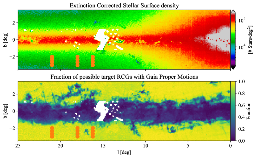
We selected fields in the bar region of the Milky Way, targeting low extinction regions close to the galactic plane, where the bar is most prominent in star counts (see footnote 6). Field centres were placed at longitudes of $l=16.2,18,21\deg$, each with latitudes of $b=-2.0,-2.33,-2.66,-3.0\deg$, for a total of 12 fields (see Figure 2).

In order to construct a clean sample of bar stars with accurate distances, we targeted standard candle RCGs for which $\sim 10\%$ accurate distances can be calculated (Bovy et al., 2014). In each field we selected stars whose extinction free ${K_{s}}$ band magnitude would place them in the bar if they were RCGs. Specifically we targeted stars whose $(H-{K_{s}})$ extinction free magnitude would place then at $\sim 4-8\,{\rm kpc}$ (i.e. we used eqn 1 of Wegg et al., 2015). To avoid biasing the sample we did not make a strict colour cut, removing only the small fraction of stars with $(H-{K_{s}})<0.06$. These stars are too blue to be RCGs even without extinction. We note that at our chosen latitudes almost all our target RCGs have Gaia astrometry available (Figures 6 and 2).

Figure 1: Upper panel: Surface density of stars with extinction corrected magnitude consistent with being red clump stars 5-8$\,{\rm kpc}$ from the Sun (specifically $13.5<\mu_{K}<14.5$ in Equation 2). Several features are notable: (i) the B/P bulge of the Milky Way in the central $10\deg;$ (ii) the higher surface density of stars at $l>0$ compared to $l<0$ outside the bulge near to the galactic plane, indicative of the extension of the bar outside the bulge; and (iii) the tilt of the galactic plane towards the edge of the plot at $|l|>70\deg,$ which is indicative of the warp/ripples in the outer disc of the Milky Way. We used near-infrared (NIR) data from the VVVsurvey (Smith et al., 2017) where available, falling back to UKIDSS-GPSdata (Lucas et al., 2008), and finally 2MASS(Skrutskie et al., 2006). After combining these three datasets only a few small regions lacked NIR of sufficient depth and these are left white. Lower panel: Fraction of stars in the upper panel which have proper motions in Gaia DR2. Outside the $\sim 1\deg$ thick dust layer in the inner Galaxy, almost all possible target RCGs have Gaia proper motions. Our selected fields, shown in red, are located in the bar outside the bulge. We show a zoom of the red dashed region containing our fields in Figure 2.

Figure 2: Zoom of footnote 6 to the region containing our fields. The 12 selected fields, shown in orange, are positioned outside the bulge close to the galactic plane where the bar is still visible in star counts, but where almost all target stars have Gaia proper motions available.

2.2 Spectral analysis

Spectra were obtained with the Fibre Large Array Multi Element Spectrograph of the Very Large Telescope at ESO (ESO/VLT/FLAMES; Pasquini et al., 2000) in the Medusa mode of the GIRAFFE multi-object spectrograph. The HR21 set-up was employed, providing a spectral coverage spanning from 8484 to 9001Å with a resolving power of $R\sim 18000$. This set-up covers the calcium triplet region and was chosen as it is also a set-up used by the Gaia-ESO Survey (GES) (Gilmore et al., 2012) and therefore facilitates comparison with other regions of the Galaxy.

The sample comprises 2456 spectra of unique stars that have a mean signal-to-noise ratio (S/N) of 40. The raw data were reduced through flat-fielding, extraction, wavelength calibration, and correction to heliocentric reference system by ESO as part of the GIRAFFE stream release.

We used the IRAF task skytweak to remove the sky emission lines from the individual spectra by adopting a median sky spectrum computed from individual spectra of dedicated fibres at each pointing. After this, we applied the continuum task to normalise the stellar continuum to the unit through a cubic spline fit. The radial velocity of each individual spectrum was derived by cross correlation against a coarse grid of synthetic templates covering the parameter space of FGK type stars. The radial velocity pipeline selects in a first iteration the best template to the observed spectrum in a $\chi^{2}$ sense, which is then used to re-compute the final radial velocity.

The set of fundamental parameters ($T_{\rm eff}$, $\log(g)$, [M/H]) and global alpha-elements enhancement [$\alpha$/Fe] were obtained by comparing the observed spectra against a grid of synthetic models. We adopted the synthetic spectral library of the GES (de Laverny et al., 2012) and the code FERRE. This code performs a global fit search for the set of fundamental parameters providing the best agreement (by minimisation of $\chi^{2}$) between the observed spectrum and the synthetic grid, allowing for interpolation between the models. During the $\chi^{2}$ minimisation search, both the models and observed spectra are re-normalised by applying a fourth-degree polynomial. This is intended to be a linear and homogeneous process (i.e. without applying any kind of iterative pixel rejection process), thereby decreasing normalisation systematic differences between observed and model spectra. We tested a couple of different strategies for re-normalisation (using a sample of GES spectra; see below) and we found that our results do not change significantly with the adopted strategy, and are of better quality than those obtained without any re-normalisation. A pixel weight mask was constructed to avoid fitting the core of Ca II triplet (CaT) lines whose modelling suffer from larger uncertainties. A number of other small spectral regions were discarded because of their systematically larger residuals, many of which are attributable to residuals of sky line subtraction.

Figure 3: Comparison of fundamental parameters and final iron abundances obtained for a sample of $\sim 600$ stars from the GES DR3. In all panels we compare the results obtained by applying to the spectra our spectral analysis procedure to those released as part of the GES DR3. In the four upper panels, we compare results for the global fundamental parameters ${\rm T_{eff}}$, ${\rm\log(g)}$, [M/H], and [$\alpha$/Fe]. In the large lower panel, we compare GES recommended metallicity with those we measured with Bacchus, both determined from iron line-by-line measurements.

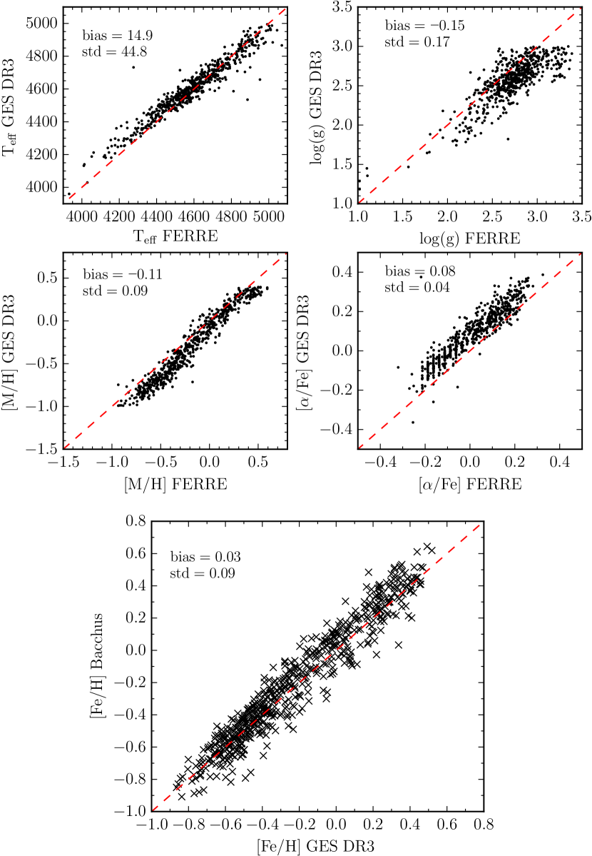
In order to verify the quality of the fitted stellar parameters and abundances obtained with our procedure, we processed a sample of spectra from the GES in the same way as our dataset. We considered stars whose set of recommended fundamental parameters (${\rm T_{eff}}$, ${\rm\log(g)}$, [M/H], [$\alpha$/Fe]), and metallicity [Fe/H] were available from the third public data release (DR3). From this, we selected a random sample of $\sim 600$ bulge giant ($\log(g)<3.0$) stars observed in the same instrumental set-up, in order to be representative of those we are studying in this work. We then ran our complete pipeline on the retrieved spectra and obtained estimates of ${\rm T_{eff}}$, ${\rm\log(g)}$, [M/H], and [$\alpha$/Fe]. In the upper panels of Figure 3 we compare our set of parameters with those of GES. There is good agreement between both sets of estimates; comparisons follow linear trends reassuringly near to the 1:1 line with small dispersion and systematic scale differences. These plots show the ability of our pipeline to produce results of comparable quality as those of the GES. We also used these comparisons to estimate the small zero points in the stellar parameters compared to GES and these are shown in the figure. We applied these zero points to calibrate the parameters of our programme stars into the astrophysical scale of the GES survey.

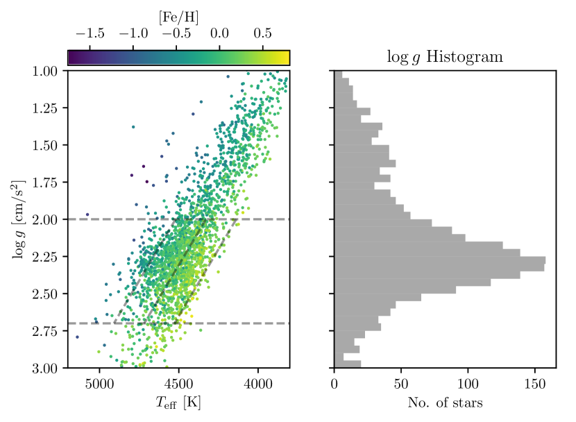
Once calibrated fundamental parameters were obtained for our programme stars, we adopted these parameters to estimate elemental abundances through line-by-line spectrum synthesis calculations using the BACCHUS code (Masseron et al., 2016). In the case of the $[{\rm Fe/H}]$ iron abundances adopted in this letter, they were computed from the mean of individual estimates over five clean Fe I lines. In the large lower panel of Fig. 3, we compare the results of this procedure applied on the $\sim 600$ test stars from the GES. The comparison between our [Fe/H] estimates and those from the GES is linear and essentially unbiased. In consideration of that, we do not apply any zero point calibration to the [Fe/H] estimates of our programme stars. In Fig. 4 we show the distribution of our programme stars in the Hertzsprung–Russell diagram, colour coded by iron abundance.

In a forthcoming paper (Rojas-Arriagada et al. in prep.) we will measure further elemental abundances beyond [Fe/H], and the complete sample and further details on our processing pipeline will be presented.

Figure 4: Left panel: Distribution of calibrated ($T_{\rm eff}$, $\log(g)$) colour coded by [Fe/H] for the entire sample. We also show the cuts used to define the sample of RCGs as dashed lines (see Equation 1); the diagonal cuts correspond from left to right to metallicities of $[{\rm Fe/H}]=-0.5,0.0,0.5$. Right panel: Histogram of the surface gravity, $\log(g)$. The peak at $\log(g)\approx 2.3$ is due to RCGs and is clear and distinct.

3 Red clump giant sample selection

Figure 5: Upper panel: Iron abundance distribution of stars within 0.5$\,{\rm kpc}$ of the bar major axis (blue) compared to those in front and behind the bar (red and green, respectively). Middle panel: Iron abundance distribution of stars in three vertical slices. The slices are chosen so each contains one-third of the sample. Lower panel: Iron abundance distribution of stars spatially in the bar, separated kinematically into bar stars (red) and inner disc stars (blue; see subsection 4.2 for details). Although these stars are in the same region of space, the stars on bar orbits are on average more metal rich than their inner disc counterparts. In black we show the iron abundance distribution of Baade’s window measured using the same instrument set-up (Schultheis et al., 2017). The highest metallicities in the bar are similar to those in the bulge, but there is a much smaller fraction of metal poor stars.

In this paper we focus our analysis on RCGs. We use RCGs because first, they are standard candles with distances accurate to $\approx 10\%$ (Bovy et al., 2014) and second, they form a very homogeneous sample, which makes differential analysis such as whether the bar is more metal rich than the disc, more straightforward. Therefore, from the sample of 2456 stars we select a clean sample of RCGs by making very similar cuts in the ($T_{\rm eff}$, $\log(g)$) plane to those described by Bovy et al. (2014) as follows:

$$2.0<\log(g)<2.7$$

$$\log(g)\leq 0.0018(T_{\rm eff}-T_{\rm eff}^{\rm ref}))+2.5$$ (1)

$$T_{\rm eff}<5000\,{\rm K,}$$

where $T_{\rm eff}^{\rm ref}=-382.5[{\rm Fe/H}]+4607\,{\rm K}$. The first of these cuts isolates clump stars in the $\log(g)$ histogram (Figure 4), while the second removes first ascent giants. We also remove stars a small number of sample stars flagged as having problems with the NIR photometry or spectroscopic fitting.

We cross match this sample of 944 stars to Gaia DR2 in which every sample star has a companion within 0.35” (footnote 6). We remove the 6 clear foreground stars whose parallax places them closer than 3$\,{\rm kpc}$ at 2$\sigma$, i.e. those with $\varpi-2\sigma(\varpi)>1/3\,{\rm kpc}$.

We do not use the Gaia parallaxes beyond this foreground cut because they provide limited information at the distance of the bar for our sample. Instead we compute distances to our stars using the distance modulus

$$\mu_{K}={K_{s}}-\overbrace{\frac{A_{K_{s}}}{E(J-{K_{s}})}\underbrace{\left[(J-{K_{s}})-(J-{K_{s}})_{\rm RC}\right]}_{\mbox{reddening}}}^{\mbox{extinction correction}}-M_{{K_{s}},{\rm RC}}\leavevmode\nobreak\ ,$$ (2)

where we adopt $M_{{K_{s}},{\rm RC}}=-1.61$ (Hawkins et al., 2017), $(J-{K_{s}})_{\rm RC}=0.68$ and $\frac{A_{K_{s}}}{E(J-{K_{s}})}=0.528$ (Gonzalez et al., 2011). An alternative approach would be to use spectro-photometric distances, however for RCGs the population corrections predicted by isochrones are highly uncertain (Girardi, 2016; Chan & Bovy, 2019). Fortunately, since RCGs are standard candles, these are at the $\sim 0.05-0.1$ level and so we adopt the more straightforward approach of Equation 2. We also checked that we find similar results using distances computed using spectro-photometric distances derived using the method of Rojas-Arriagada et al. (2017). We also checked that selecting RCGs from APOGEE DR14 and applying Equation 2 gives distances that are consistent with the spectro-photometric distances computed by Queiroz et al. (2018) with a mean absolute deviation of less than 9%. Our final sample comprises 938 RCGs stars with full 6D kinematic information together with spectroscopic iron abundance measurements.

4 Chemistry of the long bar of the Milky Way

4.1 Spatial selection of bar stars

To investigate how the chemistry of the bar compares to that of the inner disc we use the 3D position of our stars to divide the sample into three parts: (i) Those in the bar region, defined to be within $\pm 0.5\,{\rm kpc}$ of the major axis of the bar. In making this selection we assume $R_{0}=8.2\,{\rm kpc}$ (The GRAVITY Collaboration et al., 2019) and that the bar major axis lies at $27\deg$ (Wegg & Gerhard, 2013) to the Sun-galactic centre line of sight. (ii) Those in front of this bar region, but still more than $3\,{\rm kpc}$ distant from the Sun. (iii) Those behind this bar region, but still less than $10\,{\rm kpc}$ distant from the Sun. For reference, at a longitude of $l\sim 18\deg$ typical for our sample, these correspond to (i) bar stars with distance $4.6\,{\rm kpc}<d<5.8\,{\rm kpc}$, (ii) stars in front of the bar with $3\,{\rm kpc}<d<4.6\,{\rm kpc}$, and (iii) stars behind the bar with $5.8\,{\rm kpc}<d<10\,{\rm kpc}$.

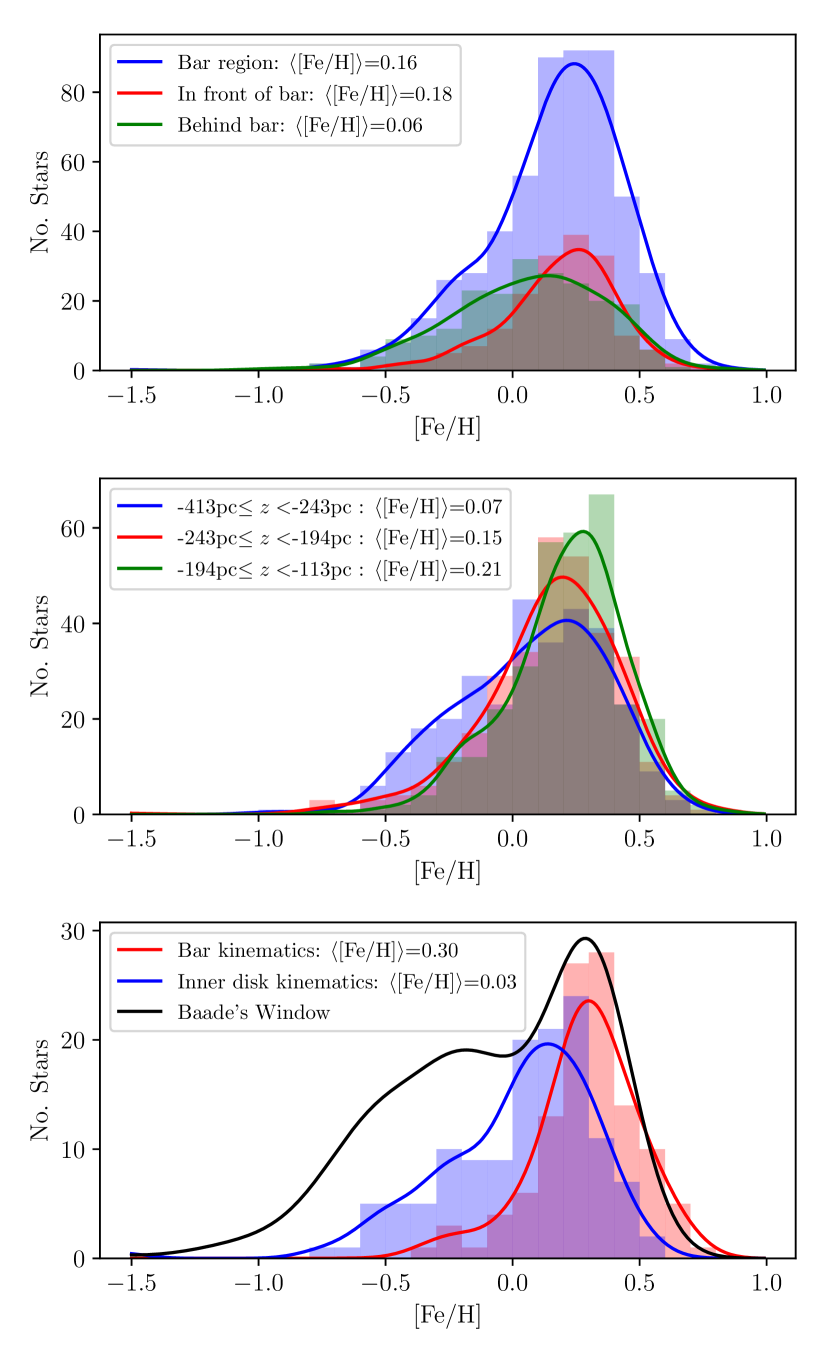
In the upper panel of Figure 5 we show the iron-abundance distribution of each of these sub-samples. We find that the metallicity distribution function (MDF) of the stars in the bar and in front of the bar are very similar, while those behind the bar are more metal poor. Quantitatively the mean $[{\rm Fe/H}]$ of the bar stars is $0.16\pm 0.01\,{\rm dex}$ compared to $0.18\pm 0.02\,{\rm dex}$ for those in front of the bar and $0.06\pm 0.02\,{\rm dex}$ for those behind.

However, we also find a very strong vertical metallicity gradient. We show the distribution of $[{\rm Fe/H}]$ in three vertical slices in Figure 5. The population of stars changes as a function of distance to the galactic plane; a higher fraction of more metal poor stars is found in the slice furthest from the galactic plane. Fitting a linear relation between $[{\rm Fe/H}]$ and distance from the galactic plane across the entire sample, the vertical gradient is $-1.1\pm 0.2\,{\rm dex}\,{\rm kpc}^{-1}$.

Because we use pencil beam fields just away from the galactic plane, our more distant stars are also on average further from the galactic plane. We must therefore account for this vertical gradient to compare the [Fe/H] distribution in the bar to the surrounding inner disc. Using the measured vertical gradient of $-1.1\,{\rm dex}\,{\rm kpc}^{-1}$ to correct our entire sample to $200\,{\rm pc}$ from the galactic plane, we find the mean $[{\rm Fe/H}]$ of the stars in the bar region is $0.18\pm 0.01\,{\rm dex}$ compared to $0.15\pm 0.02\,{\rm dex}$ for those in front of the bar and $0.15\pm 0.02\,{\rm dex}$ for those behind.

We conclude that, at the same distance from the galactic plane, the bar region in our sample is slightly more metal rich than the surrounding disc. We note that this conclusion is the opposite from that found by Bovy et al. (2019), a disagreement we discuss further in section 5.

4.2 Kinematic selection of bar stars

Figure 6: Upper panels: Kinematics of sample stars (left) and model stars (right) within 0.5$\,{\rm kpc}$ of the bar major axis. Middle panels: Model stars separated into whether they are on bar orbits (see text for details). Lower panels: The mean metallicity (left) and fraction of super solar metallicity stars (right). In the middle and lower panels we also plot the model circular velocity at these galactocentric distances (red) and orbits with zero angular momentum in a frame rotating at $\Omega=35\,{\rm km}\,{\rm s}^{-1}\,{\rm kpc}^{-1}$ (orange). These zero angular momentum orbits correspond to an pencil thin bar and have galactocentric velocity -80$\,{\rm km}\,{\rm s}^{-1}$ to 80$\,{\rm km}\,{\rm s}^{-1}$ in steps of 20$\,{\rm km}\,{\rm s}^{-1}$. In the model, bar orbits have kinematics near these low angular momentum orbits, and the stars in this region of kinematic space are preferentially metal rich.

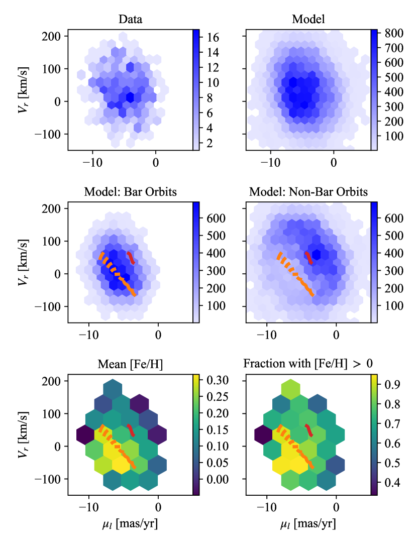
In this section we present the 2D kinematics of bar stars and make a kinematic selection of stars whose orbits indicate they follow the bar. To guide our selection and methods we use a barred made-to-measure Milky Way model of the Galaxy, which was fitted to a range of data on the inner Galaxy by Portail et al. (2017, hereafter P17). We note however, that this model was fit only to star count data in the long bar (the region studied in this work) because of the lack of kinematic data at that time. We choose to show a model with a pattern speed of $\Omega=35\,{\rm km}\,{\rm s}^{-1}\,{\rm kpc}$ because its kinematics agrees qualitatively slightly better than the fiducial model ($\Omega=40\,{\rm km}\,{\rm s}^{-1}\,{\rm kpc}$), however our conclusions would remain unchanged with any model from P17. To compare this model to our data we use the Galaxia code (Sharma et al., 2011) to generate mock catalogues of stars generated from the Padova isochrones with a 10 Gyr old population. For our fiducial MDF we use a Gaussian with $\langle[{\rm Fe/H}]\rangle=0$, $\sigma([{\rm Fe/H}])=0.3$. To these mock catalogues we apply our selection criteria, both spatially and in the ($T_{\rm eff}$, $\log(g)$) plane, to generate a mock sample of RCG stars. We also compute distances to this mock catalogue using Equation 2 in the same manner as the real sample. In the mock sample the mean absolute deviation of this RCG distance to the true distance is 6.1%. To replicate the treatment of the real sample we use these RCG distances when using the mock catalogue in what follows.

In the upper left panel of Figure 6 we show the kinematics of the stars selected to be in the bar region in the longitudinal proper motion versus radial velocity plane (i.e. $\mu_{l},V_{r}$ plane). This 2D plane encodes similar information as the well-known $(U,V)$ plane locally. We compare this to the mock sample finding qualitatively very good agreement. The sample is centred at $\mu_{l}\approx-6\,{\rm mas}\,{\rm yr}^{-1}$ similar to the $\mu_{l}=-6.24\,{\rm mas}\,{\rm yr}^{-1}$ of Sgr A* (Reid & Brunthaler, 2004). This is largely due to the motion of the Sun with respect to the galactic centre and it is reassuring for the purity of our sample that there is a complete lack of stars at $\mu_{l}>0\,{\rm mas}\,{\rm yr}^{-1}$ where nearby foreground contaminants would lie.

Using our mock sample of stars we can investigate the kinematic signatures of the bar in this 2D kinematic plane. We integrate the model stars and define long bar stars as those which spend more than 40% of their time in the long bar region; that is within $\pm 0.5\,{\rm kpc}$ of the bar major axis and more than 2$\,{\rm kpc}$ from the galactic centre. We also used the orbital frequency based definition from Portail et al. (2015) (specifically $f_{r}/f_{x}\in 2\pm 0.1$) finding very similar results. However we use the orbital time definition because it both better selects particles which were human-classified to be on bar orbits, and better photometrically separates bar stars from inner disc stars in face-on projections.

We split the model based on this orbital selection of bar stars in the middle panels of Figure 6. In these panels we also plot the position of the circular velocity for our $l=18\deg$ longitudinal field (the red line), together with the orbits of stars travelling directly along the major axis of the bar, i.e. with zero angular momentum in the co-rotating frame (orange lines). These pencil thin bar orbits cover a galactocentric radial velocity range -80$\,{\rm km}\,{\rm s}^{-1}$ to 80$\,{\rm km}\,{\rm s}^{-1}$ in steps of 20$\,{\rm km}\,{\rm s}^{-1}$. As expected, the model bar orbits lie in the region of these pencil thin orbits with a scatter due to the width of the bar and its underlying orbits (Valluri et al., 2016).

In the lower panel of Figure 6 we plot the iron abundance of our sample in the same plane. In the region of kinematic space where the bar stars lie, both the mean metallicity and the fraction of stars with super-solar abundance ($[{\rm Fe/H}]>0$) appear significantly higher.

To quantify these differences we use the $\mu_{l},V_{r}$ plane shown in Figure 6 to assign each of our sample stars a probability, $p_{\rm bar}$, that it is on a bar following orbit. We do this by for each sample star computing the fraction of bar following orbits among the 100 nearest neighbour mock sample stars in this plane. This provides a sample of stars with ($[{\rm Fe/H}]$,$p_{\rm bar}$). We use this to plot in the lower panel of Figure 5 the MDF of stars with bar orbits, $P([{\rm Fe/H}]|p_{\rm bar}=1)$, and inner disc orbits, $P([{\rm Fe/H}]|p_{\rm bar}=0)$. We compute this using a conditional kernel density estimate (KDE) $P([{\rm Fe/H}]|p_{\rm bar})=P([{\rm Fe/H}],p_{\rm bar})/P(p_{\rm bar}),$ where both probability distributions on the right-hand side are estimated using a Gaussian KDE. We also plot histograms of the stars with the highest probability to be bar stars, $p_{\rm bar}>0.8,$ and the lowest, $p_{\rm bar}<0.2$. These are very similar to the KDE estimated bar and inner disc MDFs.

Using this kinematic selection of bar stars we find that the bar is more metal rich than the inner disc with a mean iron abundance of $\langle[{\rm Fe/H}]\rangle=0.30$ compared to 0.03 for the kinematically selected inner disc stars.

5 Discussion and conclusions

We find that the bar of the Milky Way outside the B/P bulge (the so-called long bar) is more metal rich than the inner disc. We find this both kinematically and spatially selecting bar stars. The kinematic sample of bar stars is extremely metal rich with $\langle[{\rm Fe/H}]\rangle=0.30$. This MDF is comparable to the metal rich part of the MDF measured in the bulge, but unlike in the bulge, there are very few metal poor stars; only 10% of our kinematically selected bar stars have sub-solar iron abundance.

In contrast, the sample of stars selected spatially to be within the bar are only slightly more metal rich (with $\langle[{\rm Fe/H}]\rangle=0.18$ at $z=200$pc) compared to foreground and background stars (which had $\langle[{\rm Fe/H}]\rangle=0.15$). Spatially the bar and inner disc samples have a more similar mean metallicity than the kinematic selection for two reasons. First, the spatially selected samples of bar stars and inner disc stars will both contain a mixture of stars with bar orbits and inner disc orbits. Second, the distance errors are $\sim$10%, which is larger than the kinematic errors and will tend to scatter stars between the samples, reducing the contrast.

To test the consistency of our kinematic and spatial results, we therefore constructed a mock survey where the bar stars had a Gaussian MDF with $\langle[{\rm Fe/H}]\rangle=0.35$, $\sigma([{\rm Fe/H}])=0.2$ at $z=200$pc and the inner disc stars had a Gaussian MDF with $\langle[{\rm Fe/H}]\rangle=0.07$, $\sigma([{\rm Fe/H}])=0.3$ at $z=200$pc. Both populations were given a vertical gradient of $d\langle[{\rm Fe/H}]\rangle/d|z|=-1{\rm dex}/\,{\rm kpc}$ and the sample was constructed using Galaxia to sample the P17 models as described in subsection 4.2. After applying our selection function, this mock sample was analysed just as the real sample. We find that the kinematically selected bar stars in the mock sample have $\langle[{\rm Fe/H}]\rangle=0.32$ while the inner disc has $\langle[{\rm Fe/H}]\rangle=0.02$; these are very similar values to the real sample, which has $0.30$ and $0.03,$ respectively. However, the spatially selected mock sample has a much more similar mean metallicity: $0.16$ in the bar region at $z=200$pc compared to $0.12$ in front of the bar and $0.12$ behind. This simple model shows that our sample indicates that the bar is more metal rich than the inner disc in a consistent manner both when kinematically and spatially selecting bar stars.

A metal rich bar has several interesting interpretations: (i) If these stars were in place at the time of bar formation, then stars which make up the bar would preferentially sample the kinematically coolest populations (Debattista et al., 2017; Fragkoudi et al., 2017). Assuming that the inner disc at bar formation had a metallicity-age-dispersion relation analogous to that seen locally now, where young stars are preferentially metal rich with low dispersion and scale height, it would then be natural that the bar would be more metal rich than the inner disc.

However this picture is influenced by two further effects: (ii) bars in simulations grow by capturing stars from the disc over their life, particularly in the long bar region (Aumer & Schönrich, 2015). These captured stars are likely to be kinematically cool stars with guiding radii just outside the bar, a region whose stars are known to be metal rich (e.g. Hayden et al., 2015); and (iii) star formation in the bar region preferentially occurs in gas clouds that trace the bar together with associated dust lanes (Martin & Friedli, 1997). These recently formed stars are therefore preferentially be bar following and are also likely be metal rich.

Understanding the relative importance of these effects will require further data. Ages, or age indicators, in particular would help clarify if the metal rich stars formed early, together with the inner disc as expected by (i), or instead have an extended star formation history as expected by (ii) or (iii).

It is noteworthy that a bar which extends outside a B/P bulge and is more metal rich than the surrounding inner disc is also seen in our neighbouring barred galaxy, M31 (Saglia et al., 2018). This situation is also common in other nearby barred spirals (Gadotti et al., 2018).

We note that our results appear to be in disagreement with the recently submitted paper by Bovy et al. (2019) who finds that the bar is more metal poor than the surrounding disc. The reason for this apparent disagreement is unclear, but we emphasise the homogeneity of our RCG sample.

References

- Athanassoula (2005) Athanassoula, E. 2005, MNRAS, 358, 1477
- Aumer & Schönrich (2015) Aumer, M. & Schönrich, R. 2015, MNRAS, 454, 3166
- Bovy et al. (2019) Bovy, J., Leung, H. W., Hunt, J. A. S., et al. 2019, eprint arXiv:1905.11404
- Bovy et al. (2014) Bovy, J., Nidever, D. L., Rix, H.-W., et al. 2014, ApJ, 790, 127
- Bureau et al. (2006) Bureau, M., Aronica, G., Athanassoula, E., et al. 2006, MNRAS, 370, 753
- Cabrera-Lavers et al. (2008) Cabrera-Lavers, A., Gonzalez-Fernandez, C., Garzon, F., Hammersley, P. L., & Lopez-Corredoira, M. 2008, A&A, 491, 781
- Chan & Bovy (2019) Chan, V. C. & Bovy, J. 2019, arXiv e-prints, arXiv:1910.00398
- de Laverny et al. (2012) de Laverny, P., Recio-Blanco, A., Worley, C. C., & Plez, B. 2012, A&A, 544, A126
- Debattista et al. (2017) Debattista, V. P., Ness, M., Gonzalez, O. A., et al. 2017, MNRAS, 469, 1587
- Erwin & Debattista (2013) Erwin, P. & Debattista, V. P. 2013, MNRAS, 431, 3060
- Fragkoudi et al. (2017) Fragkoudi, F., Di Matteo, P., Haywood, M., et al. 2017, A&A, 606, A47
- Gadotti et al. (2018) Gadotti, D. A., Sánchez-Blázquez, P., Falcón-Barroso, J., et al. 2018, MNRAS, 482, 506
- Gilmore et al. (2012) Gilmore, G., Randich, S., Asplund, M., et al. 2012, The Messenger, 147, 25
- Girardi (2016) Girardi, L. 2016, ARA&A, 54, 95
- Gonzalez et al. (2011) Gonzalez, O. A., Rejkuba, M., Zoccali, M., Valenti, E., & Minniti, D. 2011, A&A, 534, 3
- Hammersley et al. (1994) Hammersley, P. L., Garzon, F., Mahoney, T., & Calbet, X. 1994, MNRAS, 269, 753
- Hammersley et al. (2000) Hammersley, P. L., Garzon, F., Mahoney, T. J., Lopez-Corredoira, M., & Torres, M. A. P. 2000, MNRAS, 317, L45
- Hawkins et al. (2017) Hawkins, K., Leistedt, B., Bovy, J., & Hogg, D. W. 2017, MNRAS, 471, 722
- Hayden et al. (2015) Hayden, M. R., Bovy, J., Holtzman, J. A., et al. 2015, ApJ, 808, 132
- Laurikainen et al. (2014) Laurikainen, E., Salo, H., Athanassoula, E., Bosma, A., & Herrera-Endoqui, M. 2014, MNRAS, 444, L80
- Lopez-Corredoira et al. (2005) Lopez-Corredoira, M., Cabrera-Lavers, A., & Gerhard, O. E. 2005, A&A, 439, 107
- Lopez-Corredoira et al. (2006) Lopez-Corredoira, M., Cabrera-Lavers, A., Mahoney, T. J., et al. 2006, AJ, 133, 154
- Lucas et al. (2008) Lucas, P. W., Hoare, M. G., Longmore, A., et al. 2008, MNRAS, 391, 136
- Martin & Friedli (1997) Martin, P. & Friedli, D. 1997, A&A, 326, 449
- Martinez-Valpuesta et al. (2006) Martinez-Valpuesta, I., Shlosman, I., & Heller, C. 2006, ApJ, 637, 214
- Masseron et al. (2016) Masseron, T., Merle, T., & Hawkins, K. 2016, BACCHUS: Brussels Automatic Code for Characterizing High accUracy Spectra, Astrophysics Source Code Library
- Pasquini et al. (2000) Pasquini, L., Avila, G., Allaert, E., et al. 2000, in Astronomical Telescopes and Instrumentation, ed. M. Iye & A. F. M. Moorwood (SPIE), 129
- Portail et al. (2017) Portail, M., Gerhard, O., Wegg, C., & Ness, M. 2017, MNRAS, 465, 1621
- Portail et al. (2015) Portail, M., Wegg, C., & Gerhard, O. 2015, MNRAS, 450, L66
- Queiroz et al. (2018) Queiroz, A. B. A., Anders, F., Santiago, B. X., et al. 2018, MNRAS, 476, 2556
- Reid & Brunthaler (2004) Reid, M. J. & Brunthaler, A. 2004, ApJ, 616, 872
- Rojas-Arriagada et al. (2017) Rojas-Arriagada, A., Recio-Blanco, A., de Laverny, P., et al. 2017, A&A, 601, A140
- Saglia et al. (2018) Saglia, R. P., Opitsch, M., Fabricius, M. H., et al. 2018, A&A, 618, A156
- Saito et al. (2011) Saito, R. K., Zoccali, M., McWilliam, A., et al. 2011, AJ, 142, 76
- Schultheis et al. (2017) Schultheis, M., Rojas-Arriagada, A., Garcia-Perez, A. E., et al. 2017, A&A, 600, A14
- Sharma et al. (2011) Sharma, S., Bland-Hawthorn, J., Johnston, K. V., & Binney, J. 2011, ApJ, 730, 3
- Skrutskie et al. (2006) Skrutskie, M. F., Cutri, R. M., Stiening, R., et al. 2006, AJ, 131, 1163
- Smith et al. (2017) Smith, L. C., Lucas, P. W., Kurtev, R., et al. 2017, MNRAS, 474, 1826
- The GRAVITY Collaboration et al. (2019) The GRAVITY Collaboration, Abuter, R., Amorim, A., et al. 2019, A&A, 625, L10
- Valluri et al. (2016) Valluri, M., Shen, J., Abbott, C., & Debattista, V. P. 2016, ApJ, 818, 141
- Wegg & Gerhard (2013) Wegg, C. & Gerhard, O. 2013, MNRAS, 435, 1874
- Wegg et al. (2015) Wegg, C., Gerhard, O., & Portail, M. 2015, MNRAS, 450, 4050