Gamma radiation from areal radius minima in a quasi-spherical Szekeres metric

Abstract

In previous papers it was shown that in a quasi-spherical Szekeres (QSS) metric, impulses of gamma radiation can arise that have several properties in common with the observed gamma-ray bursts. This happens when the bang-time function $t_{B}(r)$ has a gate-shaped hump around the origin of the QSS region. The gamma rays arise along two preferred directions of the QSS geometry (coincident with dipole extrema when axially symmetric, otherwise unrelated). In these directions, the rays of the relic radiation are blueshifted rather than redshifted. The blueshift is generated in a thin region between the Big Bang (BB) and the extremum-redshift hypersurface (ERH). But the Szekeres models can describe the real Universe only forward in time from the last-scattering hypersurface (LSH) because the matter in them has zero pressure. The ERH is tangent to the BB at the origin, so in a neighbourhood thereof the ERH lies earlier than the LSH and no blueshift is generated in the physical region. The question thus arose whether the BB and ERH can be “unglued” if the QSS region has no origin, but the areal radius function $\Phi$ has a local maximum or minimum somewhere. In the present paper it is demonstrated that this is indeed the case. If the hump in $t_{B}(r)$ is centered around the minimum of $\Phi$, then the BB and ERH in general do not coincide there and a stronger blueshift is generated on rays passing nearby. It follows that a lower and narrower hump on the BB set can generate sufficient blueshift to move the initial frequencies of the relic radiation to the gamma range. These facts are demonstrated by numerical calculations in an explicit example of a QSS region.

PACS numbers come here

1 Motivation and background

In previous papers [1] – [4] it was shown that flashes of gamma radiation with characteristics similar to those of the gamma-ray bursts (GRBs) [5] – [11] may arise in a Lemaître [12] – Tolman [13] (L–T) and a quasi-spherical Szekeres (QSS) model [14, 15] if the Big Bang (BB) function $t_{B}(r)$ has a suitably chosen profile in some regions. The complete model of the Universe consisted of an L–T or QSS region embedded in a $k<0$ Friedmann background; each inhomogeneous region contained an origin [16, 17]. The gamma radiation arises by blueshifting [18, 19] the light emitted at the end of the last scattering epoch along radial directions in an L–T region [1] and along two preferred directions in a QSS region [2, 3]. In Refs. [1, 3, 4] it was shown that in this way one can imitate most observed properties of the GRBs: their frequency (i.e. energy) range, the presence of afterglows, the collimation into narrow jets, the large distances to their sources, the brief durations of the bursts and their large number. However, two properties were in quantitative disagreement with the observations: the durations of the afterglows in the models were much longer than observed, and the angular radii of the sources seen by a present observer (equal to $\approx 1^{\circ}$) were larger than the localisation errors for most of the GRBs; see the last paragraph of this section for an update on this.

Refs. [1] – [4] employed models in which the energy function had the Friedmannian form $E=-\tfrac{1}{2}kr^{2}$ (with $k=-0.4$) everywhere, while the BB function $t_{B}(r)$ had a gate-shaped hump around the origin of the inhomogeneous region. The blueshift is generated in a thin slice of spacetime between the nonconstant segment of $t_{B}(r)$ [1, 3] and the etremum-redshift hypersurface (ERH) in L–T models or extremum-redshift surface (ERS) in QSS models. After crossing the ERH/ERS to the future, each ray acquires only redshift. If it were possible to observe rays emitted at the BB, and if the real Universe had the L–T or QSS geometry down to the BB, then all the blueshifted rays would display infinite blueshift to any later observer, i.e. the observed radiation would have infinite frequency. The redshift acquired after crossing the ERH/ERS could not compensate it.

However, the L–T and Szekeres models have zero pressure, so they do not apply to the earliest cosmic epochs. It is assumed that they apply toward the future from the last-scattering hypersurface (LSH) [1, 3]. (The LSH in inhomogeneous models is that on which the local mass density is equal to $\rho_{\rm LS}$ – the mass density at last scattering in the $\Lambda$CDM model, see Ref. [1] for the calculation and Eq. (15) here for the value.) The blueshift generated between the LSH and the ERH/ERS is finite, and the redshift acquired later may overcompensate it. To generate a strong blueshift, the hump on $t_{B}(r)$ should be sufficiently high and wide, but to keep the perturbations of the cosmic microwave background radiation within the limits allowed by observations, the hump should be as low and narrow as possible. These contradictive factors must be balanced to ensure that the initially generated blueshift is strong enough to survive the later redshifting while the height and diameter of the hump on $t_{B}(r)$ are within tolerable limits.

In Refs. [1] – [4] the hump on $t_{B}(r)$ was centered on the origin of the L–T or QSS region (at $r=0$ in the coordinates used there), where the ERH or ERS was tangent to the BB [1, 3]. Then, the blueshift-generating region disappears at $r=0$ and is thin (in the timelike direction) in a neighbourhood. The question thus arose whether the ERH/ERS and the BB could be “unglued”. It is shown in Appendix A that, if the hump on $t_{B}(r)$ is centered at the origin, then the unglueing of ERS and BB is possible only at the cost of shifting the BB at the origin to future infinity, which does not look realistic (somewhere in the Universe the BB would be going on forever). It still needed to be investigated whether the ERS and BB detach if the hump on the BB set is centered around a maximum or minimum of the areal radius that does not coincide with the origin. In the present paper it is demonstrated by explicit examples that this indeed happens. With the ERS and BB detached, each blueshifted ray is building up its blueshift in a longer segment of its path. Consequently, achieving the frequency range of the GRBs requires a lower or narrower hump, and the angular size of the radiation source becomes much smaller; see below. (The problem of too-long-lasting afterglows still remains and is not discussed here.)

Sections 2 and 3 present the QSS model used in this paper, the null geodesic equations and properties of redshift along them. In Sec. 4, the parameters of the QSS region around a local minimum of the areal radius are specified. In Sec. 5, a set of numerical values of the parameters of the QSS region is chosen as a starting point for improvements. In Sec. 6, the equation defining the ERS is derived and it is shown that is has a unique solution at every $r$. In Sec. 7, examples are given of QSS regions that generate sufficiently strong blueshift to reach the frequency range of the GRBs. In Sec. 8, one of the examples is further perfected to make the hump on the BB as low as possible. With the “best” parameters, the BB hump has the diameter smaller than 1/5 and the height smaller than 1/23 of that from Refs. [3, 4]. Sec. 9 investigates the numerical discrepancies between a ray calculated from the central world line of the QSS region to the present time and the same ray calculated backward from the present time to the starting point. It is shown how the discrepancies can be minimised. In Sec. 10, the angular radius of the gamma-ray source as seen by the present observer is calculated – it is $\approx 0.176^{\circ}$, and the whole sky could accommodate more than 330,000 such sources without overlaps. This fits well with the localisation errors for the 186 GRBs observed by the Large Area Telescope (LAT) from 2008 to 2018 [10], which are mostly contained between 0.04^∘ and 1.0^∘ (only 18 are greater). Sec. 11 summarises the results of this paper and prospects for improving the model.

2 The quasispherical Szekeres (QSS) spacetimes

The signature is $(+,-,-,-)$, the coordinates are $\left(x^{0},x^{1},x^{2},x^{3}\right)=(t,r,x,y)$ or $(t,r,\vartheta,\varphi)$ and we assume the cosmological constant $\Lambda=0$.

The metric of the QSS spacetimes is [14, 15, 17, 21]

$${\rm d}s^{2}={\rm d}t^{2}-\frac{\left(\Phi,_{r}-\Phi{\cal E},_{r}/{\cal E}\right)^{2}}{1+2E(r)}{\rm d}r^{2}-\left(\frac{\Phi}{\cal E}\right)^{2}\left({\rm d}x^{2}+{\rm d}y^{2}\right),\ \ \ \ \$$ (1)

$$\rm{where}\qquad{\cal E}\ {\overset{\rm def}{=}}\ \frac{S}{2}\left[\left(\frac{x-P}{S}\right)^{2}+\left(\frac{y-Q}{S}\right)^{2}+1\right],$$ (2)

$P(r)$, $Q(r)$, $S(r)$ and $E(r)$ being arbitrary functions such that $S\neq 0$ and $E\geq-1/2$ at all $r$.

The source in the Einstein equations is dust ($p=0$) with the velocity field $u^{\alpha}={\delta_{0}}^{\alpha}$. The surfaces of constant $t$ and $r$ are nonconcentric spheres, and $(x,y)$ are the stereographic coordinates on each sphere. At a fixed $r$, they are related to the spherical coordinates by

$$x = P+S\cot(\vartheta/2)\cos\varphi,$$

$$y = Q+S\cot(\vartheta/2)\sin\varphi.$$ (3)

The functions $(P,Q,S)$ determine the centres of the spheres in the spaces of constant $t$ [2, 22]. Because of the non-concentricity, the QSS spacetimes in general have no symmetry [23]. The function $\Phi(t,r)$ obeys

$${\Phi,_{t}}^{2}=2E(r)+\frac{2M(r)}{\Phi},$$ (4)

where $M(r)$ is an arbitrary function. We will consider only models with $E>0$, then the solution of (4) is

$$\Phi(t,r) = \frac{M}{2E}(\cosh\eta-1),$$

$$\sinh\eta-\eta = \frac{(2E)^{3/2}}{M}\left[t-t_{B}(r)\right],$$ (5)

where $t_{B}(r)$ is an arbitrary function; $t=t_{B}(r)$ is the time of the BB singularity, at which $\Phi(t_{B},r)=0$. We assume $\Phi,_{t}>0$ (the Universe is expanding).

The mass density implied by (1) is

$$\kappa\rho=\frac{2\left(M,_{r}-3M{\cal E},_{r}/{\cal E}\right)}{\Phi^{2}\left(\Phi,_{r}-\Phi{\cal E},_{r}/{\cal E}\right)},\quad\kappa\ {\overset{\rm def}{=}}\ \frac{8\pi G}{c^{2}}.$$ (6)

This is a mass-dipole superposed on a spherical monopole [20], [15]. The dipole vanishes where ${\cal E},_{r}=0$. The density is minimum where ${\cal E},_{r}/{\cal E}$ is maximum and vice versa [16].

The arbitrary functions must be such that no shell-crossing singularities exist. This is ensured by [16]:

$$\frac{M,_{r}}{3M} \geq \frac{\cal P}{S},\qquad\frac{E,_{r}}{2E}>\frac{\cal P}{S}~{}~{}~{}~{}\forall~{}r,$$ (7)

$${\rm where}\ \ {\cal P} \ {\overset{\rm def}{=}}\ {\sqrt{(S,_{r})^{2}+(P,_{r})^{2}+(Q,_{r})^{2}}}.$$ (8)

These inequalities imply [16]

$$\frac{M,_{r}}{3M}\geq\frac{{\cal E},_{r}}{\cal E},\qquad\frac{E,_{r}}{2E}>\frac{\Phi,_{r}}{\Phi}\qquad\forall~{}r.$$ (9)

The extrema of ${\cal E},_{r}/{\cal E}$ with respect to $(x,y)$ are [16]

$$\left.\frac{{\cal E},_{r}}{\cal E}\right|_{\rm ex}=\varepsilon_{2}\frac{\cal P}{S},\qquad\varepsilon_{2}=\pm 1,$$ (10)

with $+$ at a maximum and $-$ at minimum; they occur at

$$x=P-\frac{\varepsilon_{2}SP,_{r}}{{\cal P}+\varepsilon_{2}S},\qquad y=Q-\frac{\varepsilon_{2}SQ,_{r}}{{\cal P}+\varepsilon_{2}S}.$$ (11)

The model (1) – (2) becomes axially symmetric when $P$ and $Q$ are constant. Then, $x$ and $y$ can be chosen such that $P=Q=0$, and the set $x=y=0$ is the axis of symmetry. This is the case discussed here; then

$${\cal E}=\frac{1}{2S}\ \left(x^{2}+y^{2}+S^{2}\right).$$ (12)

In the axially symmetric case the maximally blueshifted rays stay in a fixed hypersurface (they intersect the symmetry axis in every space of constant time [2, 3]), which takes away one source of numerical errors. Without any symmetry, since the direction of strongest blueshift is unstable [2], tracing the rays would require extreme numerical precision. The form of the function $S$ is defined in Sec. 4, and conditions (7) are discussed there, too.

The following equation will be useful further on [17]:

$$\Phi,_{tr}=\frac{E,_{r}}{2E}\Phi,_{t}-\frac{M}{\Phi^{2}}\left[\left(\frac{3}{2}\frac{E,_{r}}{E}-\frac{M,_{r}}{M}\right)\left(t-t_{B}\right)-t_{B,r}\right].$$ (13)

The values of various parameters of the real Universe expressed in standard physical units are too large numbers for numerical calculations. Therefore, the numerical length unit (NLU) and the numerical time unit (NTU) were introduced in Ref. [24]:

$$1\ {\rm NTU}=1\ {\rm NLU}=3\times 10^{4}\ {\rm Mpc}=9.26\times 10^{23}\ {\rm km}=9.8\times 10^{10}\ {\rm y}.$$ (14)

The quantity $\kappa\rho$ in (6) has the dimension of (length)^-2, and in the units of (14) its value at last scattering is [1]

$$\kappa\rho_{\rm LS}=56.1294161975316\times 10^{9}\ ({\rm NLU})^{-2}.$$ (15)

In numerical calculations of past-directed null geodesics, $\kappa\rho$ is calculated along. Where its value reaches (15), that point is taken to lie on the LSH, as explained in Sec. 1, and the calculation stops.

The L–T models are the limit of (1) – (2) at constant $(P,Q,S)$. The Friedmann limit is obtained from QSS when $E/M^{2/3}$ and $t_{B}$ are constant (then $(P,Q,S)$ can be made constant by a coordinate transformation). QSS and Friedmann spacetimes can be matched at any constant $r$.

The spacetime model used further in this paper consists of a QSS region of finite spatial volume matched to a Friedmann region across a $r=r_{b}=$ constant hypersurface. The metric in the Friedmann region is

$${\rm d}s^{2}={\rm d}t^{2}-{\mathcal{R}}^{2}(t)\left[\frac{{\rm d}r^{2}}{1-kr^{2}}+r^{2}\left({\rm d}\vartheta^{2}+\sin^{2}\vartheta{\rm d}\varphi^{2}\right)\right],\ \ \ \ \$$ (16)

where the value of $k$ will be given in Sec. 4.

3 Null geodesics in the axially symmetric QSS spacetimes

In (1) – (2) $x=\infty$ and $y=\infty$ occur at the pole of the stereographic projection. This is a coordinate singularity where numerical integration of geodesics breaks down. So, we introduce the coordinates $(\vartheta,\varphi)$ by

$$x=S_{b}\cot(\vartheta/2)\cos\varphi,\qquad y=S_{b}\cot(\vartheta/2)\sin\varphi,$$ (17)

where $S_{b}$ is the value of $S$ at the Szekeres/Friedmann boundary

$$S_{b}\ {\overset{\rm def}{=}}\ S(r_{b})$$ (18)

This changes (1) and (2) to

$${\rm d}s^{2} = {\rm d}t^{2}-\frac{{\cal N}^{2}{\rm d}r^{2}}{1+2E(r)}-\left(\frac{\Phi}{\cal F}\right)^{2}\left({\rm d}\vartheta^{2}+\sin^{2}\vartheta{\rm d}\varphi^{2}\right),$$ (19)

$${\cal F} = \frac{S_{b}}{2S}\ (1+\cos\vartheta)+\frac{S}{2S_{b}}\ (1-\cos\vartheta),$$ (20)

$${\rm where} \qquad{\cal N}\ {\overset{\rm def}{=}}\ \Phi,_{r}-\Phi{\cal F},_{r}/{\cal F},$$ (21)

and the axis of symmetry is now at $\vartheta=\pi$ (where $x=y=0$) and at $\vartheta=0$ (where both $x$ and $y$ become infinite – in the stereographic coordinates this is the antipodal point to $x=y=0$).

In general, $(\vartheta,\varphi)$ are not the spherical coordinates because ${\cal F}$ depends on $\vartheta$. The dipole equator ${\cal F},_{r}=0$ is at $\cot(\vartheta_{\rm eq}/2)=S/S_{b}$. At $r=r_{b}$ ${\cal F}=1$ and $(\vartheta,\varphi)$ become the spherical coordinates with the origin at $r=0$.

In the coordinates of (19) – (20) equation (6) becomes

$$\kappa\rho=\frac{2\left(M,_{r}-3M{\cal F},_{r}/{\cal F}\right)}{\Phi^{2}\left(\Phi,_{r}-\Phi{\cal F},_{r}/{\cal F}\right)}.$$ (22)

Along a geodesic, with $\lambda$ an affine parameter, we denote

$$\left(k^{t},k^{r},k^{\vartheta},k^{\varphi}\right)\ {\overset{\rm def}{=}}\ \frac{{\rm d}{(t,r,\vartheta,\varphi)}}{{\rm d}{\lambda}}.$$ (23)

Then, the geodesic equations for (19) – (20) are

$$\frac{{\rm d}{k^{t}}}{{\rm d}{\lambda}} + \frac{{\cal N}{\cal N},_{t}}{1+2E}\left(k^{r}\right)^{2}+\frac{\Phi{\Phi,_{t}}}{{\cal F}^{2}}\left[\left(k^{\vartheta}\right)^{2}+\sin^{2}\vartheta\left(k^{\varphi}\right)^{2}\right]=0,$$ (24)

$$\frac{{\rm d}{k^{r}}}{{\rm d}{\lambda}} + 2\frac{{\cal N},_{t}}{\cal N}k^{t}k^{r}+\left(\frac{{\cal N},_{r}}{\cal N}-\frac{E,_{r}}{1+2E}\right)\left(k^{r}\right)^{2}+2\frac{S,_{r}\sin\vartheta\Phi}{S{\cal F}^{2}{\cal N}}\ k^{r}k^{\vartheta}$$ (25)

$$- \frac{\Phi(1+2E)}{{\cal F}^{2}{\cal N}}\left[\left(k^{\vartheta}\right)^{2}+\sin^{2}\vartheta\left(k^{\varphi}\right)^{2}\right]=0,$$

$$\frac{{\rm d}{k^{\vartheta}}}{{\rm d}{\lambda}} + 2\frac{\Phi,_{t}}{\Phi}k^{t}k^{\vartheta}-\frac{S,_{r}\sin\vartheta{\cal N}}{S\Phi(1+2E)}\ \left(k^{r}\right)^{2}+2\frac{\cal N}{\Phi}k^{r}k^{\vartheta}$$ (26)

$$+ \frac{{\cal F},_{\vartheta}}{\cal F}\ \left[-\left(k^{\vartheta}\right)^{2}+\sin^{2}\vartheta\left(k^{\varphi}\right)^{2}\right]-\cos\vartheta\sin\vartheta\left(k^{\varphi}\right)^{2}=0,$$

$$\frac{{\rm d}{k^{\varphi}}}{{\rm d}{\lambda}} + 2\frac{\Phi,_{t}}{\Phi}k^{t}k^{\varphi}+2\frac{\cal N}{\Phi}k^{r}k^{\varphi}+2\left[\frac{\cos\vartheta}{\sin\vartheta}-\frac{{\cal F},_{\vartheta}}{\cal F}\right]k^{\vartheta}k^{\varphi}=0.$$ (27)

The geodesics determined by (24) – (27) are null when

$$\left(k^{t}\right)^{2}-\frac{{\cal N}^{2}\left(k^{r}\right)^{2}}{1+2E(r)}-\left(\frac{\Phi}{\cal F}\right)^{2}\left[\left(k^{\vartheta}\right)^{2}+\sin^{2}\vartheta\left(k^{\varphi}\right)^{2}\right]=0.$$ (28)

On past-directed rays $k^{t}<0$, and $\lambda$ along each of them can be chosen such that at the observation point

$$k^{t}_{o}=-1.$$ (29)

(On future-directed rays $k^{t}>0$ and a convenient choice of $\lambda$ is $k^{t}_{e}=+1$.)

In the Friedmann region we choose the coordinates so that [1]

$$S=S_{b}.$$ (30)

Then, throughout the Friedmann region, ${\cal F}=1$ and $(\vartheta,\varphi)$ are the spherical coordinates. They coincide with the coordinates of the QSS region at $r=r_{b}$.

To calculate $k^{r}$ on nonradial rays, (28) will be used, which is insensitive to the sign of $k^{r}$. This sign will be changed by the numerical program integrating {(24), (26) – (28)} at each point where $k^{r}$ reaches zero.

Note that $\vartheta\equiv 0$ and $\vartheta\equiv\pi$ are solutions of (26). These axial rays intersect every space of constant $t$ on the symmetry axis.

Along a ray emitted at $P_{e}$ and observed at $P_{o}$, with $k^{\alpha}$ being affinely parametrised, we have

$$1+z=\frac{\left(u_{\alpha}k^{\alpha}\right)_{e}}{\left(u_{\alpha}k^{\alpha}\right)_{o}},$$ (31)

where $u_{\alpha}$ are four-velocities of the emitter and of the observer [25]. In our case, both the emitter and the observer comove with the cosmic matter, so $u_{\alpha}={\delta^{0}}_{\alpha}$, and the affine parameter is chosen so that (29) holds; then

$$1+z=-{k_{e}}^{t}.$$ (32)

Equation (27) has the first integral:

$$k^{\varphi}\sin^{2}\vartheta\Phi^{2}/{\cal F}^{2}=J_{0},$$ (33)

where $J_{0}$ is constant along each geodesic. Using (33), eq. (28) implies

$$(k^{t})^{2}=\frac{{\cal N}^{2}\left(k^{r}\right)^{2}}{1+2E}+\left(\frac{\Phi}{\cal F}\right)^{2}\left(k^{\vartheta}\right)^{2}+\left(\frac{J_{0}{\cal F}}{\sin\vartheta\Phi}\right)^{2}.$$ (34)

At the observation/emission point, (29)/(32), respectively, apply. Equations (34) and (32) show that for rays emitted at the BB, where $\Phi=0$, the observed $z$ is infinite when $J_{0}\neq 0$. A necessary condition for infinite blueshift ($1+z_{o}=0$) is thus $J_{0}=0$, so

(a) either $k^{\varphi}=0$,

(b) or $\vartheta=0,\pi$ along the ray ((33) implies $J_{0}/\sin\vartheta\to 0$ when $\vartheta\to 0,\pi$).

Condition (b) appears to be also sufficient, but so far this has been demonstrated only numerically in concrete examples of QSS models ([2, 3]).

Condition (a) is not sufficient, and Ref. [2] contains numerical counterexamples: there exist rays that proceed in a surface of constant $\varphi$, but approach the BB with $z\to\infty$; the value of $\vartheta$ along them changes and is different from $0,\pi$. For those rays, (34) with $J_{0}=0$ implies one more thing

$${\rm If\ }\lim_{t\to t_{B}}z=\infty\ {\rm and}\ \lim_{t\to t_{B}}\left|k^{r}\right|<\infty$$

$${\rm then}\ \lim_{t\to t_{B}}k^{\vartheta}=\pm\infty,$$ (35)

i.e., such rays approach the BB tangentially to the surfaces of constant $r$.

Consider a ray proceeding from event $P_{1}$ to $P_{2}$ and then from $P_{2}$ to $P_{3}$. Let the redshifts acquired in the intervals $[P_{1},P_{2}]$, $[P_{2},P_{3}]$ and $[P_{1},P_{3}]=[P_{1},P_{2}]\cup[P_{2},P_{3}]$ be $z_{12}$, $z_{23}$ and $z_{13}$, respectively. Then, from (31),

$$1+z_{13}=\left(1+z_{12}\right)\left(1+z_{23}\right).$$ (36)

Thus, for a ray proceeding to the past from $P_{1}$ to $P_{2}$, and then back to the future from $P_{2}$ to $P_{1}$:

$$1+z_{12}=\frac{1}{1+z_{21}}.$$ (37)

4 Relations around a spatial minimum of $\Phi(t,r)$

For the metric (1) – (2), in the orthonormal tetrad of differential forms:

$${\rm e}^{0} = {\rm d}t,\quad\quad{\rm e}^{1}=\frac{F}{\sqrt{1+2E}}\ {\rm d}r,\quad{\rm e}^{2}=\frac{\Phi}{\cal E}\ {\rm d}x,\quad{\rm e}^{3}=\frac{\Phi}{\cal E}\ {\rm d}y,\ \ \ \ \$$ (38)

$${\rm where} \ F\ {\overset{\rm def}{=}}\ \Phi,_{r}-\Phi{\cal E},_{r}/{\cal E},$$ (39)

the tetrad components of the curvature tensor are

$$R_{0101}=\frac{2M}{\Phi^{3}}-\frac{M,_{r}-3M{\cal E},_{r}/{\cal E}}{\Phi^{2}F},$$ (40)

$$R_{0202}=R_{0303}=\frac{1}{2}\ R_{2323}=-\frac{M}{\Phi^{3}},$$ (41)

$$R_{1212}=R_{1313}=\frac{M}{\Phi^{3}}-\frac{M,_{r}-3M{\cal E},_{r}/{\cal E}}{\Phi^{2}F}.$$ (42)

These are scalars, so any scalar polynomial in curvature components is determined by them.

The metric (1) has a singularity where $F=0$, but as seen from the above, this will not be a curvature singularity if $M,_{r}-3M{\cal E},_{r}/{\cal E}$ has there a zero of the same order. Such a location is either a neck (where $2E+1=0$ of the same order) [17, 16] or a local spatial extremum of $\Phi$. In those cases, $F=0$ is just a coordinate singularity.

For a neck to exist, $E$ must be negative in its neighbourhood. To consider this case, we would have to either take a different background $E$ from those considered in Refs. [1] – [4] (where $E$ was positive and Friedmannian) or allow the sign of $E$ to vary within the QSS region. In the first case, we would give up on the correspondence with the previous papers, the second case would introduce an additional complication. So, for this exploratory investigation, we will consider a spatial extremum of $\Phi(t,r)$.

The equations $F=0$ and $M,_{r}-3M{\cal E},_{r}/{\cal E}=0$ can be simultaneously fulfilled only if, at that location,

$$M,_{r}=E,_{r}=P,_{r}=Q,_{r}=S,_{r}={{{\rm d}{t_{B}}}/{{\rm d}{r}}}=0,$$ (43)

and then the extremum is comoving with the cosmic dust [17, 16]. All zeros must be of the same order. If the extremum does not coincide with the origin $\Phi=0$, then $M$ at it must be nonzero – see (2).

The metric (1) – (2) is covariant with transformations of the form $r=f(r^{\prime})$, where $f$ is an arbitrary function. Consequently, we can choose $r$ such that the extremum is at $r=0$. Suppose that all the zeros in (43) are of order $(n-1)$, where $n\geq 2$ is a natural number to be chosen later. The simplest $M$, $E$, $t_{B}$ and $S$ with this property have the following form:

$$M = M_{\rm ext}+Dr^{n},$$ (44)

$$E = E_{\rm ext}+Ar^{n},$$ (45)

$$t_{B} = t_{\rm Bext}-Br^{n},$$ (46)

$$S = \sqrt{r^{n}+a^{n}},$$ (47)

where the subscript “e” stands for “at extremum of $\Phi$”, and all the symbols newly introduced here are constants. The signs in (44) – (46) were chosen such that $D$, $A$ and $B$ are all positive for a spatial minimum of $\Phi$ at $r=0$. Also, $M_{\rm ext}=M(0)>0$ (because $M>0$ always) and $E_{\rm ext}=E(0)>0$ because we now follow the $E>0$ model. The form of $S$ was chosen for correspondence with Refs. [2, 3, 4] when $n=2$. We shall consider a minimum because this leads to simpler formulae (a maximum is left for a later paper, if anybody cares to write it).

For a spatial minimum of $\Phi$, a neighbourhood of $r=0$ exists in which, at a fixed $t=t_{o}$, $\Phi,_{r}>0$. Then, to avoid shell crossings in this neighbourhood, the following conditions must be obeyed ([16] with $P=Q=0$):

$$M,_{r}>0,\qquad E,_{r}>0,\qquad t_{B,r}<0,\ \ \ \ \$$ (48)

$$\frac{S,_{r}}{S}<\frac{M,_{r}}{3M},\qquad\frac{S,_{r}}{S}<\frac{E,_{r}}{2E}.$$ (49)

Since $M>0$ and we assume $E>0$ (for correspondence with earlier papers), the equations above imply

$$D>0,\qquad A>0,\qquad B>0,$$ (50)

$$M_{\rm ext}<\tfrac{1}{3}\ D\left(2a^{n}-r^{n}\right),\qquad E_{\rm ext}<Aa^{n}.$$ (51)

Somewhere in the range of $r$ determined by (51), the QSS region will be matched to a Friedmann background, where $E(r)=-\tfrac{1}{2}\ kr^{2}$ and $M(r)=M_{0}r^{3}$, with constant $k$ and $M_{0}$. Let the matching hypersurface be $r=r_{b}$. Since $r\leq r_{b}$ in the QSS region, a sufficient condition for the first of (51) is

$$M_{\rm ext}<\tfrac{1}{3}\ D\left(2a^{n}-{r_{b}}^{n}\right).$$ (52)

The value of $k$ is in principle arbitrary, but, for correspondence (we wish to have the same Friedmann background as in Refs. [1] – [4]), we choose

$$k=-0.4.$$ (53)

Also for correspondence, we choose

$$M_{0}=1\ {\rm NLU}.$$ (54)

At the QSS/Friedmann boundary we must thus have

$$E_{\rm ext}+A{r_{b}}^{n} = -\tfrac{1}{2}\ k{r_{b}}^{2},$$ (55)

$$M_{\rm ext}+D{r_{b}}^{n} = M_{0}{r_{b}}^{3}.$$ (56)

The $M_{\rm ext}$ and $D$ must be chosen in agreement with (52) and (56), and for $E_{\rm ext}$ consistency between (51) and (55) imposes the condition

$$E_{\rm ext}=-\tfrac{1}{2}\ k{r_{b}}^{2}-A{r_{b}}^{n}<Aa^{n},$$ (57)

which is equivalent to

$$A>\frac{-\frac{1}{2}\ k{r_{b}}^{2}}{{r_{b}}^{n}+a^{n}}\ {\overset{\rm def}{=}}\ {\overline{A}}.$$ (58)

5 The initial choice of parameter values

As a test of the model, the numerical calculation of blueshift on the rays emitted at the spatial minimum of $\Phi(t,r)$ was at first done with the values of the parameters in the QSS region that were not too different from those in the previous papers [1, 3]. The QSS/Friedmann boundary is here at $r=r_{b}$, and in Ref. [3] it was at

$$r=B_{1}+A_{1}=0.015+10^{-10},$$ (59)

so a realistic first choice is

$$r_{b}=0.015.$$ (60)

The BB time at $r=0$ is here $t_{\rm Bext}$, at $r=r_{b}$ it is $t_{\rm Bext}-B{r_{b}}^{n}$. The difference, $B{r_{b}}^{n}$, is the height of the hump on the BB. In Ref. [3], the height was

$$B_{0}+A_{0}=0.000126\ {\rm NTU}\ {\overset{\rm def}{=}}\ H.$$ (61)

So, we impose the condition

$$B{r_{b}}^{n}=H.$$ (62)

All these conditions now have to be made into a self-consistent set. So, the initial prescription for constructing a QSS region free of shell crossings around a spatial minimum of $\Phi$ is:

($i$) Select $n$. We choose $n=6$, since in previous papers the BB profile was a curve of degree 6.

($ii$) Choose $r_{b}=0.015$, as in (60).

($iii$) With $H$ given by (61), $B$ is

$$B=H/{r_{b}}^{n}=11\ 061\ 728.395061729\ {\rm NTU}.$$ (63)

($iv$) Choose $a^{n}$. We take it the same as $a^{2}$ in the previous papers:

$$a^{n}=0.001.$$ (64)

($v$) Choose $A>{\overline{A}}$ in agreement with (58). We choose

$$A=0.05.$$ (65)

With $k=-0.4$, $n=6$ and $r_{b}\leq 0.015$, the ${\overline{A}}$ defined in (58) has ${{\rm d}{\overline{A}}}/{{\rm d}{r_{b}}}>0$. Consequently, when $r_{b}$ is made smaller, $A=0.05$ will fulfil (58) with a wider margin. With $k$, $r_{b}$ and $A$ already defined, we obtain from (57)

$$E_{\rm ext}=4.4999999430468751\times 10^{-5}.$$ (66)

This obeys $E_{\rm ext}<Aa^{n}$ since $Aa^{n}=5\times 10^{-5}$. Similarly to what happens with ${\overline{A}}$, with the values of $n$, $k$ and $A$ given above, $E_{\rm ext}$ is an increasing function of $r_{b}$. Consequently, (57) will be fulfilled with $r_{b}<0.015$.

($vi$) Choose $D>0$. There is no other condition on $D$, so we take

$$D=1\ {\rm NLU}.$$ (67)

($vii$) Now $M_{\rm ext}$ is determined by (56). With the already-chosen values of $M_{0}$, $r_{b}$ and $D$ we have

$$M_{\rm ext}=3.3749886093750001\times 10^{-6}\ {\rm NLU},$$ (68)

while $M_{u}\ {\overset{\rm def}{=}}\ \tfrac{1}{3}D\left(2a^{n}-{r_{b}}^{n}\right)=0.0006666666628697916...$, so (52) is obeyed. Also, ${{\rm d}{M_{\rm ext}}}/{{\rm d}{r_{b}}}>0$ while $M_{u}$ becomes greater when $r_{b}$ decreases, so with $r_{b}<0.015$ $M_{\rm ext}$ will be smaller than (68) and will continue to obey (52).

As in [1] – [4], for the BB time in the Friedmann background we take

$$t_{\rm Bf}=-0.13945554689046649\ {\rm NTU}\approx-13.67\times 10^{9}\ {\rm years};$$ (69)

see Ref. [4] for justification. So,

$$t_{\rm Bext}=t_{\rm Bf}+H=-0.13932954689046649\ {\rm NTU}.$$ (70)

Caution must be exercised while calculating $k^{r}$ from (28). If $r=0$ is not a neck, then, with the $r$-coordinate used so far, ${\cal N}|_{r=0}=0$, but $1+2E|_{r=0}\neq 0$ and $\left.k^{r}\right|_{r=0}$ comes out infinite. Therefore, in using this equation, one must change the $r$-coordinate to $\overline{r}=r^{n}$, at least in a neighbourhood of $r=0$. Thus, the order of zero of the derivatives in (43) is in fact irrelevant: one can do the transformation $\overline{r}=r^{n}$, and then $r^{\prime}={\overline{r}}^{1/m}$ with any $m\neq n$ – the resulting $\Phi,_{r^{\prime}}$ will have a zero at $r^{\prime}=0$ of order $m\neq n$, but the metric will be just a coordinate transform of the original one. However, with a changed $n$ the values of the other parameters of the QSS region will be also changed.

6 The Extremum Redshift Surface

Consider a null geodesic that stays in one of the two surfaces:

$$\{\cos\vartheta,\varphi\}=\{-\varepsilon,{\rm constant}\},$$ (71)

where $\varepsilon=\pm 1$, i.e., $\vartheta=\pi$ or $\vartheta=0$, respectively. Such geodesics obey (26) and (27) provided the limit $\varphi=$ constant in (27) is taken first. Along the direction $\vartheta=\pi$ ($\varepsilon=+1$) the dipole is maximum, along the other one ($\vartheta=0,\varepsilon=-1$) it is minimum.

All along such a geodesic, $k^{r}\neq 0$ because wherever $k^{r}=0$ the geodesic would be timelike, so $r$ can be used as a parameter. Assume the geodesic is past-directed so that (32) applies. Then we obtain from (24) using (32)

$$\frac{{\rm d}{z}}{{\rm d}{r}}=\frac{{\cal N}{\cal N},_{t}}{1+2E}\ k^{r}.$$ (72)

Since ${\cal N}\neq 0$ from no-shell-crossing conditions [16] and $k^{r}\neq 0$, the extrema of $z$ on such a geodesic occur where

$${\cal N},_{t}\equiv\Phi,_{tr}-\Phi,_{t}{\cal F},_{r}/{\cal F}=0.$$ (73)

In deriving (73), the constant $\varphi$ was arbitrary. Thus, the set defined by (73) is 2-dimensional; it is the Extremum Redshift Surface (ERS) [2].

With (71) obeyed, ${\cal F},_{r}/{\cal F}=\varepsilon S,_{r}/S$. Using (13), Eq. (73) becomes

$$\left(\frac{E,_{r}}{2E}-\varepsilon\frac{S,_{r}}{S}\right)\Phi,_{t}-\frac{M}{\Phi^{2}}\left[\left(\frac{3}{2}\frac{E,_{r}}{E}-\frac{M,_{r}}{M}\right)\left(t-t_{B}\right)-t_{B,r}\right]=0.$$ (74)

Substituting for $\Phi$, $\Phi,_{t}$ and $(t-t_{B})$ from (2), Eq. (74) is transformed to

$$\sqrt{2E}\left[\left(\frac{E,_{r}}{2E}-\varepsilon\frac{S,_{r}}{S}\right)\sinh\eta\cosh\eta+\left(-2\frac{E,_{r}}{E}+\frac{M,_{r}}{M}+\varepsilon\frac{S,_{r}}{S}\right)\sinh\eta\right.$$

$$+\left.\left(\frac{3}{2}\frac{E,_{r}}{E}-\frac{M,_{r}}{M}\right)\eta\right]+\frac{(2E)^{2}}{M}\ t_{B,r}=0.\ \ \$$ (75)

This is the equation of the ERS. In the limit $S,_{r}=0$ it reproduces the equation of the Extremum Redshift Hypersurface (ERH) of Ref. [27].

Equation (75) implies that, with $S(r)$ given by (47), the ERS coincides with the BB at the origin $r=r_{\rm or}$ if and only if $\lim_{r\to r_{\rm or}}\left[(r-r_{\rm or}){{\rm d}{t_{B}}}/{{\rm d}{r}}\right]=0$; see Appendix A. Consequently, the two sets are “unglued” at $r=r_{\rm or}$ if and only if $\lim_{r\to r_{\rm or}}\left[(r-r_{\rm or}){{\rm d}{t_{B}}}/{{\rm d}{r}}\right]=C\neq 0$. Then, in a neighbourhood of the origin, the function $t_{B}(r)$ behaves like [$-\ln(r-r_{\rm or})$], so $\lim_{r\to r_{\rm or}}t_{B}(r)=\infty$. This means that somewhere in the Universe the BB would be still going on now (and would go on forever). Whether this is “plausible” or not, such a geometry deserves to be investigated, see footnote 3.

Substituting (44) – (47) in (75) and canceling $nr^{n-1}$ we obtain

$${\cal H}(r,\eta)=F_{4}(r),$$ (76)

where

$${\cal H}(r,\eta) = F_{1}(r)\sinh\eta\cosh\eta+F_{2}(r)\sinh\eta+F_{3}(r)\eta,$$ (77)

$$F_{1}(r) = \frac{A}{E_{\rm ext}+Ar^{n}}-\frac{\varepsilon}{r^{n}+a^{n}}\equiv\frac{(1-\varepsilon)Ar^{n}+Aa^{n}-\varepsilon E_{\rm ext}}{\left(E_{\rm ext}+Ar^{n}\right)\left(r^{n}+a^{n}\right)},$$ (78)

$$F_{2}(r) = -\frac{4A}{E_{\rm ext}+Ar^{n}}+\frac{2D}{M_{\rm ext}+Dr^{n}}+\frac{\varepsilon}{r^{n}+a^{n}}\ ,\ \ \ \$$ (79)

$$F_{3}(r) = \frac{3A}{E_{\rm ext}+Ar^{n}}-\frac{2D}{M_{\rm ext}+Dr^{n}}\ ,$$ (80)

$$F_{4}(r) = \frac{2^{5/2}\left(E_{\rm ext}+Ar^{n}\right)^{3/2}B}{M_{\rm ext}+Dr^{n}}.$$ (81)

Taking (76) at $r=0$ we see that $\eta=0$ fulfils it only when $E_{\rm ext}B=0$ – only then the ERS coincides with the BB at the BB extremum. If we wish to unglue these two sets at that point, we must take $BE_{\rm ext}\neq 0$ in (45) – (46). Our choice (63) and (66) guarantees this.

Extrema of redshift exist also along other directions than $\vartheta=0$ and $\vartheta=\pi$, as was demonstrated by numerical examples in Refs. [1] – [4], but a general equation defining their loci remains to be derived.

With the values of the parameters in (60) – (70), one can verify that ${\cal H}>0$ and ${\partial{\cal H}}/{\partial{\eta}}>0$ for all $\eta>0$, see Appendix B. Since $F_{4}(r)>0$ for all $r>0$ and is independent of $\eta$, the following is true: at $\eta=0$, ${\cal H}=0<F_{4}(r)$ for all $r>0$, at $\eta\to\infty$, ${\cal H}\to+\infty$, so ${\cal H}>F_{4}(r)$ at all finite $r>0$ for sufficiently great $\eta$. Thus, somewhere in the range $\eta\in(0,\infty)$ Eq. (76) has a unique solution for $\eta$ at any finite $r>0$. The initial $\eta>0$ for the numerical program solving (76) is found also in Appendix B.

7 The numerical values of blueshift

The formulae in Secs. 4 and 5 presented those features of the QSS region that will not vary between numerical experiments. This section presents the first numerical implementation and its consecutive improvements. The aim of the whole action is to (1) achieve the lowest possible value of $1+z$ with a given set of parameters by fine-tuning the point where the ray intersects the $r=0$ line, and then (2) decrease the diameter and height of the BB hump as much as possible while keeping $1+z$ in the range [1]

$$2.56\times 10^{-8}<1+z<1.689\times 10^{-5}$$ (82)

needed to blueshift the emission frequencies of hydrogen and helium atoms (the dominating matter components in the epoch of last scattering) to the range of frequencies of the observed GRBs. The lower end of this range corresponds to the highest-frequency emission radiation being blueshifted to the highest energy of the observed GRBs, the upper end of (82) corresponds to matching the lowest-frequency ends of the two bands. The aim of the current paper is to find out how low and thin the BB hump can be made while (82) still holds.

7.1 Model 1

With the numerical values of the parameters given in Secs. 4 and 5, a light ray running in the surface (71) with $\varepsilon=+1$, sent to the past from $r=0$ at $t=t_{B}(0)+\Delta t_{c1}$, where

$$\Delta t_{c1}=0.00000449960000\ {\rm NTU},$$ (83)

crossed the LSH with

$$1+z_{p1}=8.1259273421174782\times 10^{-8}$$ (84)

relative to the initial point. Achieving a still smaller $1+z$ was probably possible, but would require extreme numerical precision to correctly catch the $(t,r)$ point where the ray intersects the LSH (this is because the ray and the LSH intersect at a very small angle, see Fig. 1). The result (84) was comparable to the best one achieved in Ref. [3] and was good enough as a starting point for improvements of the BB profile.

A ray sent from the same initial point to the future, in the surface $\{\vartheta,\varphi\}=\{0,{\rm constant}\}$, reached the present time with

$$1+z_{f1} = 55.299746938015609,$$

$$t_{\rm now1} = 5.0391335364848865\times 10^{-11}\ {\rm NTU},$$

$$r_{\rm now1} = 0.89044002852488546.$$ (85)

In the following, the concatenation of the two rays described above will be called Ray 1. On it, the blueshift between the LSH and $t_{\rm now1}$ was

$$1+z_{t1}=\left(1+z_{f1}\right)\times\left(1+z_{p1}\right)=4.49361725656\times 10^{-6}.$$ (86)

This is $\approx 0.2855$ of the value obtained with a BB hump of the same height and nearly the same diameter but centered around the origin (Eq. (8.12) in Ref. [3]). Thus, a BB hump around a spatial minimum of $\Phi$ generates blueshifts more efficiently than a similar hump around the origin. The reason for this is explained at the end of the present section.

7.2 Model 2

In the second numerical experiment, the radius of the BB hump was decreased to $r_{b2}=0.01$, which changed the values of $M_{\rm ext}$, $E_{\rm ext}$ and $B$ to

$${\rm second}\ M_{\rm ext} = 10^{-6}-10^{-12},$$

$${\rm second}\ E_{\rm ext} = 0.00001999999995,$$

$${\rm second}\ B = 1.26\times 10^{8}.$$

The other parameters did not change, and, as predicted in Sec. 5, the inequalities (52) and (57) still held. On a ray sent to the past from $r=0$ in the direction of dipole maximum ((71) with $\vartheta=\pi$) the parameter $\Delta t_{c2}$ that resulted in the smallest $1+z$ at the LSH was

$$\Delta t_{c2}=0.00000133331600\ {\rm NTU},$$ (87)

and the smallest $1+z$ was

$$1+z_{p2}=7.5237815977402533\times 10^{-11}.$$ (88)

The ray sent to the future from the same initial point in the direction of the dipole minimum ($\vartheta=0$) overshot the present time by $t_{\rm now2}$ given below. The parameters of the endpoint were

$$1+z_{f2} = 56.981145007279054,$$ (89)

$$t_{\rm now2} = 4.3253430781086085\times 10^{-10}\ {\rm NTU},$$ (90)

$$r_{\rm now2} = 0.88867576379669344.$$ (91)

The total blueshift between the LSH and $t_{\rm now2}$ was thus

$$1+z_{t2}=4.2871369\times 10^{-9}.$$ (92)

In the following, the concatenation of these two rays will be called Ray 2.

7.3 Model 3

In the third numerical experiment, $r_{b}$ was decreased to $r_{b3}=0.005$. The new values of $M_{\rm ext}$, $E_{\rm ext}$ and $B$ became

$${\rm third}\ M_{\rm ext} = 1.24999984375\times 10^{-7},$$

$${\rm third}\ E_{\rm ext} = 9.9999999921875\times 10^{-7},$$

$${\rm third}\ B = 8.064\times 10^{9},$$

which again preserved (52) and (57). The past-directed ray sent from $r=0$ in the surface (71) along $\vartheta=\pi$ had the smallest $1+z$ at the LSH when

$$\Delta t_{c3}=0.00000016666400\ {\rm NTU};$$ (93)

and the blueshift on it at the LSH was

$$1+z_{p3}=1.8781317501215256\times 10^{-8}.$$ (94)

The ray sent to the future from the same initial point in the direction of the dipole minimum $(\vartheta=0)$ overshot the present time by $t_{\rm now3}$, with

$$1+z_{f3} = 73.679048074068589,$$ (95)

$$t_{\rm now3} = 5.0921478176623031\times 10^{-10}\ {\rm NTU},\ \ \ \$$ (96)

$$r_{\rm now3} = 0.88725616206450841.$$ (97)

The total $z$ between the LSH and $t_{\rm now3}$ was thus

$$1+z_{t3}=1.383789595\times 10^{-6}.$$ (98)

The concatenation of these two rays will be called Ray 3.

Further experiments with decreasing $r_{b}$ were not carried out because at $r_{b}=0.005$ a numerical instability, known from previous papers [1, 2], showed up: at $\Delta t_{c}$ slightly larger than (93), the past-directed ray overshot the BB hump and hit the BB in the Friedmann region far from the QSS region, while at $\Delta t_{c}$ slightly smaller than (93), the past-directed ray hit the BB close to $r=0$ with $1+z$ larger than the upper limit in (82).

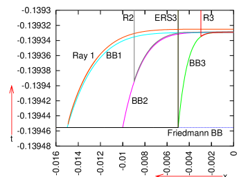
Figure 1: The segments of Rays 1 – 3 between the LSH and $r=0$, and their corresponding BB profiles. The coordinate $x=-r$ goes along the dipole maximum. See more explanation in the text.

Figure 1 shows Rays 1, 2 and 3 between $r=0$ and the LSH, and their corresponding BB profiles. The dipole maximum is to the left, at $\vartheta=\pi$. The curves BB1, BB2 and BB3 are the graphs of $t_{B}(r)$ corresponding to $r_{b}=0.015$, $r_{b}=r_{b2}=0.01$ and $r_{b}=r_{b3}=0.005$, respectively. The vertical lines R2 and R3 mark the $x=-r$ coordinates of the points where Rays 2 and 3, respectively, crossed the LSH. The LSH for each profile is, at the scale of the figure, indistinguishable from the BB. The line ERS3 is at the outer edge of the Extremum Redshift Surface corresponding to BB3. Between $r=0$ and $r=r_{b3}$, this surface lies high above the BB hump and nearly horizontally: its $t$-coordinate varies from 890.8421697 NTU at $r=0$ to 890.8421435 NTU at $r=r_{b3}$. This is high above the upper edge of Fig. 1. Consequently, all axial rays keep acquiring blueshift as long as they stay in the QSS region - unlike in Refs. [1, 2], where the ERS was tangent to the BB at the origin. For this reason, a minimum of $\Phi$ generates a stronger blueshift than an inhomogeneity around the origin, as is seen by comparing (86), (92) and (98) with $1+z=1.553\times 10^{-5}$ obtained in Ref. [3].

8 Decreasing the height of the BB hump

Figure 2 shows a closeup view on Ray 3 and BB3 of Fig. 1. As is seen, Ray 3 flew above the BB hump only for about half of the hump’s radius; the remaining part of the inhomogeneity did not influence it. Thus, a stronger blueshift could be achieved by moving the ray up so that it hits the BB hump still further down. But our ultimate aim is to give the hump the smallest possible angular diameter as seen by the present observer. Therefore, in the next step we lowered the BB hump without changing the ray parameters.

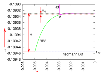
Figure 2: The segment of Ray 3 between the LSH and $r=0$, and the BB3 profile. The vertical line R3 marks the value of $x=-r$ at which Ray 3 crossed the LSH. More explanation in the text.

The part of the QSS region to the left of the R3 line did not contribute to the blueshift on Ray 3, so we replaced it by the Friedmann background. Ray 3 crossed the LSH at point A in Fig. 2, with $(t,r)=(t_{A},r_{A})$, where

$$t_{A} = -0.13933481010992060\ {\rm NTU},$$

$$r_{A} = 2.9452138001815902\times 10^{-3}.$$ (99)

The $r_{A}$ was taken as the new outer boundary of the QSS region, while $t_{\rm Bf}$ and $B$ of (69) and (63) were left the same. After this, the height of the BB hump decreased from the $H$ of (61) to

$$H_{4}=t_{\rm Bf}+H-t_{A}=5.26321945411\times 10^{-6}\ {\rm NTU},$$ (100)

see Fig. 2. Then, a past-directed Ray 4 was calculated from the initial point $(r_{4},t_{4})\ {\overset{\rm def}{=}}\ (0,t_{\rm Bf}+H_{4}+\Delta t_{c3})$ with $\Delta t_{c3}$ as in (93) along $\vartheta=\pi$. The blueshift on it on crossing the LSH was

$$1+z_{p4}=1.8786236899437370\times 10^{-8},$$ (101)

very close to that of (94). Figure 3 shows the corrected BB configuration and the past-directed part of Ray 4.

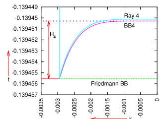
Figure 3: The BB profile with the boundary between the QSS and Friedmann regions being at point A of Fig. 2. The vertical straight line marks the value of $x=-r$ at which the ray crossed the LSH.

On the ray propagating from $(r_{4},t_{4})$ upward to the present time along $\vartheta=0$ the $r_{b}$ parameter had to be changed from $r_{b3}$ to $r_{A}$. The redshift on it between $r=0$ and the present time came out to be

$$1+z_{f4}=458.91884554506117.$$ (102)

Consequently, the total $1+z$ between the LSH and the present time was

$$1+z_{t4}=\left(1+z_{p4}\right)\left(1+z_{f4}\right)=0.862135815\times 10^{-5}.$$ (103)

This is safely within the range defined by (82). This $z_{t4}$ was achieved with the radius of the BB hump (as measured by $r$) and its height $H_{4}$ being 0.196 and 0.042, respectively, of those in Ref. [4].

In consequence of numerical inaccuracies, the future endpoint of Ray 4 overshot the present time $t=0$. The coordinates of the endpoint were

$$t_{\rm now4} = 7.6253109886207342\times 10^{-11}\ {\rm NTU},\ \ \ \$$ (104)

$$r_{\rm now4} = 0.95434899416269714.$$ (105)

For completeness, a similar operation to that described above was done on the BB2 profile. The QSS/Friedmann boundary was moved from $r_{b}=r_{b2}=0.01$ to $r=r_{b5}$, slightly beyond the $r$ at which Ray 2 crossed the LSH:

$$r_{b5}=0.0090765667.$$ (106)

The corresponding $t$ on BB2 is

$$t_{b5}=-0.1394\ {\rm NTU}.$$ (107)

This resulted in replacing the $H$ of (61) by

$$H_{5}=t_{\rm Bf}+H-t_{b5}=7.04531\times 10^{-5}\ {\rm NTU}.$$ (108)

The ray sent to the future from $(r,t)=(0,t_{\rm Bf}+H_{5}+\Delta t_{c2})$ (the same $\Delta t_{c2}$ as in (87)) is Ray 5 from Fig. 4. As the other rays, it overshot the present time by $t_{\rm now5}$, and the parameters of the endpoint were

$$1+z_{f5} = 84.123779615683631,$$ (109)

$$t_{\rm now5} = 8.6312831305632174\times 10^{-10}\ {\rm NTU},\ \ \ \$$ (110)

$$r_{\rm now5} = 0.90628860720677851.$$ (111)

The total $1+z$ between the LSH and $t_{\rm now5}$ was thus, from (88) and (109),

$$1+z_{t5}=\left(1+z_{p2}\right)\left(1+z_{f5}\right)=6.32928945\times 10^{-9}.$$ (112)

This is much better than the lower end of the range (82).

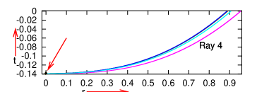
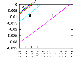
Figure 4: Upper panel: Rays 1 – 5 shown from the LSH to the present time. The arrow points to the graph of the BB3 profile, which is the tiny dot. Lower panel: The same rays near their upper ends. The difference in $r$ between the center of the BB hump and the observer is largest for Ray 4 and smallest for Ray 3.

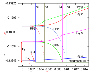
Figure 5: The segments of Rays 2 – 5 going from $r=0$ toward the present time, shown in and near the QSS region, and their corresponding BB profiles.

Figure 4 shows the $t(r)$ graphs of Rays 1 – 5 all along their length (the upper panel) and near their upper ends (the lower panel).

Figure 5 shows the segments of Rays 2 – 4 between $r=0$ and $r=0.015$, and their corresponding BB profiles. Between the LSH and $r=0$, Ray 3 has the same shape as Ray 4 and would coincide with it when translated down by $H-H_{4}$. Similarly, Ray 2 would coincide with Ray 5 between the LSH and $r=0$ when translated down by $H-H_{5}$. The same is true for the pairs of BB profiles (BB4, BB3) and (BB5, BB2).

9 Tracing the rays back from the present time

In the next section we will calculate the angular radius of the QSS region corresponding to BB4 as seen by the observer at $t=0$ who receives the maximally blueshifted gamma ray. For this purpose, we will have to integrate (24) – (28) backward in time from the observer position and find the ray that grazes the boundary of the QSS region. But we must verify whether the observer position was correctly identified, i.e., whether the axial ray emitted from the endpoint of Ray 4 at $t=0$ toward the past coincides with Ray 4 at $r=0$. As will be seen below, it does not: the two rays nearly coincide between $t=0$ and the QSS/Friedmann boundary, but the backward ray (hereafter called IR 4, short for “inverse Ray 4”) enters the QSS region with a different ${{\rm d}{t}}/{{\rm d}{r}}$ than Ray 4 had on leaving it. This problem, caused by numerical inaccuracies, existed also in Refs. [3, 4]. The present section explains how this discrepancy was handled.

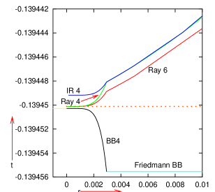
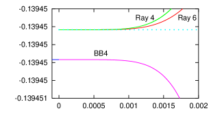
Figure 6: Upper panel: Rays 4, 6 and IR 4 in a vicinity of the BB4 hump. The dotted line marks the $t$-coordinate of Ray 4 at $r=0$. The difference between this $t$ and the top of BB4 is the $\Delta t_{c3}$ of (93). The $t$-coordinates of Rays 6 and 4 at $r=0$ differ by 0.12% of $\Delta t_{c3}$, see text. Lower panel: A closeup view on the neighbourhood of $(t,r)=(t_{B}(0)+\Delta t_{c3},0)$ in the upper panel. The difference between Rays 4 and 6 at $r=0$ is not visible at the scale of this figure. Ray IR 4 is above the upper edge of the figure.

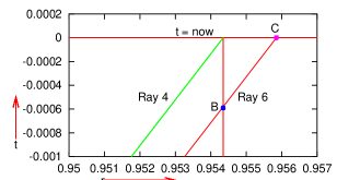
Figure 7: Rays 4 and 6 in a vicinity of the present time $t=0$. The difference between $t=0$ and the actual values of $t$ on the upper ends of the two rays is not visible at the scale of the figure. The vertical line marks the $r$-coordinate on Ray 4 at the present time. The meaning of points B and C is explained in Appendix C.

The IR 4 was sent from $(t,r)=(t_{\rm now4},r_{\rm now4})$ given by (104) – (105), and arrived at $r=0$ with $t$ differing visibly from that of Ray 4, see the upper panel of Fig. 6. The $t(0)-t_{B}(0)$ on IR 4 was $\approx 6.6\times\Delta t_{c3}$ instead of $\Delta t_{c3}$ for Ray 4 given by (93). So, the initial point of the past-directed ray was hand-corrected so as to achieve a better coincidence at $r=0$. On Ray 6 shown in Fig. 6, the ratio $(t(0)-t_{B}(0))/\Delta t_{c3}$ was $\approx 0.9988$, and it was taken to be a satisfactory precision. The initial point of Ray 6 is at

$$t_{\rm now6} = 1.9143125092526522\times 10^{-11}\ {\rm NTU},\ \ \ \$$

$$r_{\rm now6} = 0.95585224106471711.$$ (113)

Appendix C explains how this point was found. The $1+z$ on Ray 6 between the point of coordinates (9) and $(t(0),0)$ was 568.65551516257369 – rather strongly off the value (102), but this discrepancy has no influence on the calculation of the angular radius in the next section. The real redshift along this geodesic segment should be between these values. Figure 7 shows Rays 4 and 6 in a vicinity of the present time $t=0$. The real $r$-coordinate of the observer receiving the ray with the strongest blueshift should be between $r_{\rm now4}$ of (105) $r_{\rm now6}$ of (9). We will calculate the angular radius of the light source for both these positions of the observer.

See Appendix D for remarks on numerical precision.

10 The angular size of the source of the blueshifted rays

To determine the angular radius of the QSS region seen by a present observer one has to shoot a past-directed ray from the observer position in such a direction that it grazes the boundary of the inhomogeneity, call it Ray T. This ray was found by trial and error. Then the angle $\alpha$ between Ray T and the axial ray (the one that passes through $r=0$) is the desired angular radius. As shown in Ref. [3] it is given by

$$\cos\alpha=\sqrt{1-\left(k^{\vartheta}_{o}\Phi_{o}\right)^{2}}\Longrightarrow\sin\alpha=k^{\vartheta}_{o}\Phi_{o},$$ (114)

where $k^{\vartheta}_{o}$ is the $\vartheta$ component of the vector $k^{\alpha}$ tangent to Ray T at the observer and $\Phi_{o}$ is the value of the metric function $\Phi$ at the observer. This calculation was done for two observer positions: the initial point of Ray 6 given by (9) and the endpoint of Ray 4 given by (104) – (105). The difference is not significant: the angular radius for the first observer is

$$\alpha_{1}=0.00308221\ {\rm rad}=0.1765976^{\circ},$$ (115)

and for the second observer it is

$$\alpha_{2}=0.0030774\ {\rm rad}=0.1763199^{\circ};$$ (116)

the corresponding rays are denoted T1 and T2 in Figs. 8 and 9. In Ref. [3], the angular radius of the QSS region around the origin was between 0.96767^∘ and 0.9681^∘, depending on the direction of observation. Whichever combination of two radii we take, the ratio of the radius found here to that in Ref. [3] is $\approx 0.182$. The difference between (115) and (116) is influenced by the numerical error in determining the impact parameter of the ray relative to $r=0$. For the first observer this parameter is $0.9976\times r_{b}$, for the second one it is $0.9968\times r_{b}$. These numbers show that the “grazing” rays actually entered the QSS region a little. However, the redshift on them between the LSH and the present time does not significantly differ from that on the ray that stayed in the Friedmann region all the way. On two all-Friedmannian rays reaching the first observer, $1+z$ was

$$951.55845651643119\quad{\rm and}\quad 951.56113626862839,$$ (117)

while on the “grazing” rays the respective values were 951.56298581163151 and 951.63204672978486. On Ray P, for which the impact parameter was $0.96\times r_{b}$ the redshift was $1+z=1026.4529080967900$, i.e., $z$ was larger than on the grazing rays. This is consistent with what was found in Ref. [3]: on decreasing the impact parameter from the edge of the QSS region, $z$ at first increased above the background value before it started to decrease. Figures 8 and 9 show Rays T1, T2 and P in two views.

The angular radii (115) and (116) are smaller than the angular resolution for most of the 186 GRBs detected by the LAT between 2008 and 2018 [10]: the localisation error was smaller than 0.18^∘ in 55 cases.

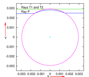
Figure 8: Projection of the rays that graze the QSS region on a surface of constant $t$ along the flow lines of the dust filling the spacetime. The boundary of the QSS region is the large circle. Rays T1 and T2 correspond to the two positions of the observer described in the text; at the scale of this figure they coincide. Ray P is a projection of an exemplary ray that penetrates the QSS region. The coordinates in the figure are $(X,Y)=r(\cos\vartheta,\sin\vartheta)$, with $(r,\vartheta)$ being those of (24) – (28).

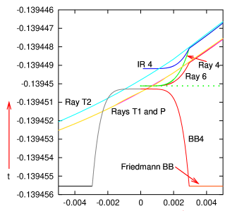
Figure 9: This is a modified version of Fig. 6, which includes the rays shown in Fig. 8. The nonaxial rays T1, T2 and P are shown here projected on the $Y=0$ surface along lines of constant $t$ and $X$.

An interesting question now is: how many circles of angular radius $\alpha$ can be placed on the celestial sphere without overlapping? A method to tackle this question was suggested in Ref. [3]. We imagine each circle being inscribed into a quadrangle of arcs of great circles on a sphere $S_{c}$ of radius $R_{c}$, and then divide the surface area of $S_{c}$ by the surface area of the quadrangle. The resulting number $N$ is only an approximate estimate because such shapes cannot completely cover the sphere: the quadrangles will leave holes between them. However, this method takes into account some of the area outside the circles, so it yields a better approximation than dividing $4\pi{R_{c}}^{2}$ by the surface area of the small circle. By Ref. [3],

$$N=\frac{\pi}{\arcsin\left(\sin^{2}\alpha\right)}.$$ (118)

Taking $\alpha=0.00308221$ rad, the result is

$$N=330\ 694,$$ (119)

which is $\approx 30$ times the number for QSS regions that contain an origin [3].

11 Conclusion

In the previous papers [3] – [4], QSS regions possessing origins were employed to consider the same process as the one considered here: matter inhomogeneities blueshifting (along preferred directions) rays of the relic radiation from their initial frequencies to the gamma range. The conclusion of the present paper is: when the QSS region does not possess an origin, but surrounds a spatial minimum of the areal radius function $\Phi$, then it may be a few times smaller in diameter and its amplitude of $t_{B}(r)$ may be several times lower, and yet it will generate gamma rays of the same frequency range. The angular radius of the gamma-ray source seen by the present observer is here between $0.176^{\circ}$ and $0.177^{\circ}$, which is $\approx 0.182<1/5$ of that in the previous papers. The amplitude of the bang-time function $t_{B}(r)$ (the $H_{4}$ in (100)) is here $\approx 0.042<1/23$ of that in Refs. [3] – [4]. The reason of the improvement is that the extremum redshift surface is tangent to the BB at an origin (the case considered in the former papers), but is not tangent to it at the minimum of $\Phi$ (the case considered here). Consequently, in the present case light rays passing through the QSS region spend more time in the blueshift-generating zone. This is why a smaller inhomogeneity around a minimum of $\Phi$ is needed to generate the same range of blueshift.

It must be strongly emphasised that $\alpha_{1}$ and $\alpha_{2}$ given in (115) and (116) are NOT the lower bounds on the angular radii of sources of gamma rays. The inhomogeneity that produced these numbers is an example – a proof of existence of a sufficiently small source of the gamma radiation, and no optimisation was attempted. So, it must be possible to make it still smaller. It would be incredible to find the absolute minimum of diameter and amplitude by blind search – and the same is true for the configurations considered in Ref. [3]. Thus, there is room for further improvements (for example by allowing the $E(r)$ function to be non-Friedmannian).

Depending on the shape of the $t_{B}(r)$ function, the rays emitted from the last-scattering hypersurface as hydrogen and helium emission radiation may be blueshifted to different bands, not necessarily to the gamma-ray frequencies. For example, they may end up reaching the present observers as X- or ultraviolet rays. In the latter cases the required blueshifts would be weaker ($z$ would not have to be as close to $-1$ as in (82)), so lower and narrower humps on the BB would suffice. Consequently, reconciling these inhomogeneities with the observed limits on anisotropies of the CMB radiation (directional temperature differences $\Delta T/T\approx 10^{-5}$) would be easier. The reason why Refs. [1] – [4] and the present paper concentrated on blueshifting to the gamma range is just because this is the most difficult case. This author did not wish to be suspected of choosing the easy ways.

The papers [1] – [4] and the present one discussed only the conditions for blueshifting the initial frequencies to the GRB range. The questions of the expected present intensity of the blueshifted radiation and of its spectrum were not considered, and the answers to them are crucial for the problem of detectability. This will have to be dealt with in the future; it might happen that in our real Universe the signal is too weak to be detected at present. But the right time to consider detectability will come when we clearly understand what kind of signal should be expected, and this is what the papers were meant to clarify.

Appendix A When do ERS and BB coincide at the origin?

Equations (74) and (75) were derived without using any explicit choice of the $r$-coordinate (no use was made of (44) – (46)). So, in this appendix we can choose $r$ so that $r=0$ at the origin, not at an extremum, and $M=M_{0}r^{3}$. We recall that with such choice of $r$, and with $P=Q=0$ and $S$ given by (47) the origin is nonsingular when [16, 17]

$$E=-\tfrac{1}{2}\ kr^{2}+{\cal O}_{2}(r)\qquad\left(\Longrightarrow E,_{r}=-kr+{\cal O}_{1}(r)\right),$$ (120)

where ${\cal O}_{\ell}(r)$ denotes a function that has the property

$$\lim_{r\to 0}\frac{{\cal O}_{\ell}(r)}{r^{\ell}}=0$$ (121)

for $\ell\geq 0$ (with $\ell=0$ this means $\lim_{r\to 0}{\cal O}_{0}(r)=0$). No approximations will be used along the way – the whole calculation will be exact, but the explicit forms of the functions hidden in ${\cal O}_{\ell}(r)$ will be irrelevant.

Substituting $M=M_{0}r^{3}$ and (120) in (75) we obtain

$$\left[\left(\frac{-kr+{\cal O}_{1}(r)}{-kr^{2}+2{\cal O}_{2}(r)}-\frac{1}{2}\ \frac{\varepsilon nr^{n-1}}{r^{n}+a^{2}}\right)\sinh\eta\cosh\eta\right.$$

$$+\left(\frac{3}{r}-2\frac{-kr+{\cal O}_{1}(r)}{-\tfrac{1}{2}kr^{2}+{\cal O}_{2}(r)}+\frac{1}{2}\ \frac{\varepsilon nr^{n-1}}{r^{n}+a^{2}}\right)\sinh\eta$$

$$+\left.\left(\frac{3}{2}\ \frac{-kr+{\cal O}_{1}(r)}{-\tfrac{1}{2}kr^{2}+{\cal O}_{2}(r)}-\frac{3}{r}\right)\eta\right]\times\sqrt{-kr^{2}+2{\cal O}_{2}(r)}$$

$$+\frac{\left(-kr^{2}+2{\cal O}_{2}(r)\right)^{2}}{M_{0}r^{3}}\ \frac{{\rm d}{t_{B}}}{{\rm d}{r}}=0.$$ (122)

Now we factor out $r$ from $\sqrt{-kr^{2}+2{\cal O}_{2}(r)}$ and multiply by $r$ each term in the long square bracket. We note that $\lim_{r\to 0}{\cal O}_{2}/r^{2}=\lim_{r\to 0}{\cal O}_{1}/r=0$, so

$$\lim_{r\to 0}\left(\frac{-kr^{2}+r{\cal O}_{1}(r)}{-kr^{2}+2{\cal O}_{2}(r)}\right)=1,$$ (123)

$$\lim_{r\to 0}\left[\frac{\left(-kr^{2}+2{\cal O}_{2}(r)\right)^{3/2}}{M_{0}r^{3}}\right]=\frac{(-k)^{3/2}}{M_{0}}.$$ (124)

Then, in the limit $r\to 0$, (A) becomes

$$4\sinh^{3}(\eta_{0}/2)\cosh(\eta_{0}/2)+\frac{(-k)^{3/2}}{M_{0}}\ \lim_{r\to 0}\left(r\ \frac{{\rm d}{t_{B}}}{{\rm d}{r}}\right)=0,$$ (125)

where $\eta_{0}=\lim_{r\to 0}\eta$. This shows that $\eta_{0}=0$ (i. e., the ERS and BB coincide at the origin) if and only if $\lim_{r\to 0}\left(r{{\rm d}{t_{B}}}/{{\rm d}{r}}\right)=0$. $\square$

Appendix B Solvability of Eq. (76)

The second line of (78) shows that when $\varepsilon=+1$, $F_{1}(r)>0$ in consequence of (57). When $\varepsilon=-1$, $F_{1}(r)>0$ in consequence of $A>0$ and $E_{\rm ext}>0$, see the comment under (47).

From (77) we see that $\left.{\cal H}\right|_{\eta=0}=0$. Further

$$\frac{\partial{\cal H}}{\partial{\eta}}=2F_{1}\cosh^{2}\eta+F_{2}\cosh\eta+F_{3}-F_{1}.$$ (126)

From here,

$$\left.\frac{\partial{\cal H}}{\partial{\eta}}\right|_{\eta=0} = F_{1}+F_{2}+F_{3}=0,$$ (127)

$$\frac{\partial{{}^{2}{\cal H}}}{\partial{\eta^{2}}} = \sinh\eta\ \left(4F_{1}\cosh\eta+F_{2}\right).$$ (128)

Now we define

$${\cal G}(r,\eta)\ {\overset{\rm def}{=}}\ 4F_{1}\cosh\eta+F_{2},$$ (129)

and find, using (78) and (79)

$$\left.{\cal G}\right|_{\eta=0}=4F_{1}+F_{2}=\frac{2Da^{n}+(2-3\varepsilon)Dr^{n}-3\varepsilon M_{\rm ext}}{\left(M_{\rm ext}+Dr^{n}\right)\left(r^{n}+a^{n}\right)}.$$ (130)

When $\varepsilon=-1$, this is obviously positive in consequence of $D$ and $M_{\rm ext}$ being positive, see the comment under (47). When $\varepsilon=+1$, this is positive in consequence of the first of (51), so

$${\cal G}(0)>0,$$ (131)

$$\frac{\partial{\cal G}}{\partial{\eta}}=4F_{1}\sinh\eta,$$ (132)

which is positive for all $\eta>0$ in consequence of $F_{1}(r)>0$.

Consequently, ${\cal G}(r,\eta)>0$ for all $\eta\geq 0$, so ${\partial{{}^{2}{\cal H}}}/{\partial{\eta^{2}}}>0$ for all $\eta>0$. Then, from (127), ${\partial{\cal H}}/{\partial{\eta}}>0$ for all $\eta>0$. Since $\left.{\cal H}\right|_{\eta=0}=0$, this means ${\cal H}>0$ for all $\eta>0$.

The numerator of $F_{3}$ is $F_{3{\rm n}}=A\left(3M_{\rm ext}+Dr^{n}\right)-2DE_{\rm ext}\leq A\left(3M_{\rm ext}+D{r_{b}}^{n}\right)-2DE_{\rm ext}$ since $r\leq r_{b}$. Substituting for $M_{\rm ext}$ from (56) and for $E_{\rm ext}$ from (57), we obtain $F_{3{\rm n}}\leq 3AM_{0}{r_{b}}^{3}+Dk{r_{b}}^{2}$. With the values of $A$, $M_{0}$, $r_{b}$, $D$ and $k$ given in (65), (54), (60), (67) and (53), $3AM_{0}{r_{b}}^{3}+Dk{r_{b}}^{2}<0$, so $F_{3}<0$ ((51) alone did not guarantee this).

To find an initial $\eta$ for a numerical program solving (76), we use (127) to write (77) in the form

$${\cal H}=F_{1}(r)\sinh\eta(\cosh\eta-1)-F_{3}(r)(\sinh\eta-\eta).$$ (133)

Now we observe that, for all $\eta>0$,

$$\cosh\eta-1>\eta^{2}/2,\qquad\sinh\eta>\eta,$$

$$\sinh\eta-\eta>\eta^{3}/6.$$ (134)

Since $F_{3}<0$, (133) and (B) imply that for all $\eta>0$,

$${\cal H}>\left(F_{1}/2-F_{3}/6\right)\eta^{3}\ {\overset{\rm def}{=}}\ {\cal H}_{i}.$$ (135)

Hence, every $\eta$ that solves (76) is smaller than the $\eta_{i}$ that solves ${\cal H}_{i}=F_{4}(r)$. Thus, $\eta_{i}$ can be used as the initial upper limit on $\eta$ in solving (76) by the bisection method. The lower limit is $\eta=0$ since we showed that $F_{4}(r)>0$ for all $r$, while ${\cal H}=0$ at $\eta=0$.

Appendix C Determining the upper end of Ray 6

Since the IR 4 ray reached $r=0$ too high above the BB, the whole ray had to be moved down. In the first step, the $r$-coordinate of the reverse ray was retained, but its $t$ coordinate was lowered by $\Delta t_{1}\ {\overset{\rm def}{=}}\ \Delta T\times(1+z_{f4})$, where $1+z_{f4}$ is given by (102) and $\Delta T$ is the difference between $t(0)$ on IR 4 and the desired $t(0)$ on Ray 4. The discrepancy decreased, but was still too large. So the next values of the initial $t$ at $r_{\rm now4}$ were tested by trial and error, by adding numerical coefficients to $\Delta t_{1}$. After a few corrections, the coincidence shown in Fig. 6 was achieved with $\Delta t_{2}\approx-6.47358\times 10^{-6}$ NTU; the initial point of the fine-tuned reverse ray is point B in Fig. 7. Then, a future-directed axial ray was sent from point B, and it intersected the $t=0$ surface at point C in Fig. 7. Actually, the ray again overshot $t=0$ slightly, and the coordinates of its endpoint are

$$t = 1.9143125092526522\times 10^{-11}\ {\rm NTU},$$

$$r = 0.95585224106471711.$$ (136)

This became the initial point of the past-directed Ray 6, given by (9).

Appendix D Remarks on numerical precision

To calculate the geodesics with a high precision, the numerical step in the affine parameter, $\Delta\lambda$, should be as small as possible. But when it is small, a single run of a numerical program lasts prohibitively long. A compromise had to be struck. Between the LSH and $r=0$ on Rays 1, 3 and 4 the step was $\Delta\lambda=10^{-9}$, in the same segment on Rays 2 and 5 it was $\Delta\lambda=10^{-6}$. On the segments of rays between $r=0$ and the present time $t=0$, $\Delta\lambda$ was $10^{-8}$ on Ray 1 and $10^{-7}$ on Rays 2, 3 and 5.

Ray 4 was designed to be the representative one, so its segment between $r=0$ and the present time was calculated with a higher precision. On it, the initial $\Delta\lambda$ at $r=0$ was $10^{-17}$, then it was multiplied by 100 at each of $r=0.0004$, 0.0005, 0.002, 0.005 and 0.07. The reason of this changing $\Delta\lambda$ is that $1+z=k^{t}={{\rm d}{t}}/{{\rm d}{\lambda}}$, so where $z$ is large (resp. small), $t$ changes by large (resp. small) increments of $\Delta t=(1+z)\Delta\lambda$. On a future-directed geodesic, the initial $z=0$ and decreases along the way, so after a while $\Delta t$ becomes very small and the calculation proceeds exceedingly slowly, requiring a huge number of numerical steps.

The reverse occurs on past-directed geodesics: $\Delta\lambda$ must be decreased along the way, or else increasing $z$ damages the precision. On Ray 6, the initial $\Delta\lambda$ at $(t,r)_{\rm now6}$ was $10^{-9}$, then it was divided by 100 at each of $r=$ 0.07, 0.005, 0.002, 0.0005 and 0.0004.

For the nonaxial rays grazing the QSS region, considered in Sec. 10, a different scheme of changes in $\Delta\lambda$ had to be applied because they leave the Friedmann region for only a brief time and cover larger segments of $r$, so too high a precision would result in prohibitively long integration times. On them, the initial $\Delta\lambda$ was $10^{-9}$, and it was divided by 100 at each of $x=$ 0.17 and 0.002.

Acknowledgement For some calculations, the computer algebra system Ortocartan [28, 29] was used.

References

- [1] A. Krasiński, Cosmological blueshifting may explain the gamma ray bursts. Phys. Rev. D93, 043525 (2016).
- [2] A. Krasiński, Existence of blueshifts in quasi-spherical Szekeres spacetimes. Phys. Rev. D94, 023515 (2016).
- [3] A. Krasiński, Properties of blueshifted light rays in quasispherical Szekeres metrics. Phys. Rev. D97, 064047 (2018).
- [4] A. Krasiński, Short-lived flashes of gamma radiation in a quasi-spherical Szekeres metric. ArXiv 1803.10101, not to be published.
- [5] S. B. Cenko et al., Afterglow observations of Fermi large area telescope gamma-ray bursts and the emerging class of hyper-energetic events. Astrophys. J. 732, 29 (2011).
- [6] A. Goldstein et al., The Fermi GBM gamma-ray burst spectral catalog: the first two years. Astrophys. J. Suppl. 199, 19 (2012).
- [7] D. Gruber et al., The Fermi GBM gamma-ray burst spectral catalog: four years of data. Astrophys. J. Suppl. 211, 12 (2014).
- [8] P. Kumar and B. Zhang, The physics of gamma-ray bursts & relativistic jets. Phys. Rep. 561, 1 – 109 (2015).
- [9] S. J. Smartt, A twist in the tale of the -ray bursts. Nature 523, 164 (2015).
- [10] M. Ajello et al., A Decade of Gamma-Ray Bursts Observed by Fermi-LAT: The Second GRB Catalog. Astrophys. J. 878, 52 (2019).
-
[11]
BATSE All-Sky Plot of Gamma-Ray Burst Locations,
https://heasarc.gsfc.nasa.gov/docs/cgro/cgro/batse_src.html - [12] G. Lemaître, L’Univers en expansion [The expanding Universe]. Ann. Soc. Sci. Bruxelles A53, 51 (1933); English translation: Gen. Relativ. Gravit. 29, 641 (1997); with an editorial note by A. Krasiński: Gen. Relativ. Gravit. 29, 637 (1997).
- [13] R. C. Tolman, Effect of inhomogeneity on cosmological models. Proc. Nat. Acad. Sci. USA 20, 169 (1934); reprinted: Gen. Relativ. Gravit. 29, 935 (1997); with an editorial note by A. Krasiński, in: Gen. Relativ. Gravit. 29, 931 (1997).
- [14] P. Szekeres, A class of inhomogeneous cosmological models. Commun. Math. Phys. 41, 55 (1975).
- [15] P. Szekeres, Quasispherical gravitational collapse. Phys. Rev. D12, 2941 (1975).
- [16] C. Hellaby and A. Krasiński. You cannot get through Szekeres wormholes: Regularity, topology and causality in quasi-spherical Szekeres models. Phys. Rev. D66, 084011 (2002).
- [17] J. Plebański and A. Krasiński, An Introduction to General Relativity and Cosmology. Cambridge University Press 2006, 534 pp, ISBN 0-521-85623-X.
- [18] P. Szekeres, Naked singularities. In: Gravitational Radiation, Collapsed Objects and Exact Solutions. Edited by C. Edwards. Springer (Lecture Notes in Physics, vol. 124), New York, pp. 477 – 487 (1980).
- [19] C. Hellaby and K. Lake, The redshift structure of the Big Bang in inhomogeneous cosmological models. I. Spherical dust solutions. Astrophys. J. 282, 1 (1984) + erratum Astrophys. J. 294, 702 (1985).
- [20] M. M. de Souza, Hidden symmetries of Szekeres quasi-spherical solutions, Revista Brasileira de Física 15, 379 (1985).
- [21] C. Hellaby, The nonsimultaneous nature of the Schwarzschild singularity. J. Math. Phys. 37, 2892 (1996).
- [22] R. G. Buckley and E. M. Schlegel, Physical geometry of the quasispherical Szekeres models. Phys. Rev. D101, 023511 (2020).
- [23] W. B. Bonnor, A. H. Sulaiman and N. Tomimura, Szekeres’s space-times have no Killing vectors, Gen. Rel. Grav. 8, 549 (1977).
- [24] A. Krasiński, Accelerating expansion or inhomogeneity? Part 2: Mimicking acceleration with the energy function in the Lemaître – Tolman model. Phys. Rev. D90, 023524 (2014).
- [25] G. F. R. Ellis, Relativistic cosmology. In Proceedings of the International School of Physics “Enrico Fermi”, Course 47: General relativity and cosmology. Edited by R.K. Sachs, Academic Press, 1971, pp. 104-182. Reprinted: Gen. Relativ. Gravit. 41, 581 (2009); with an editorial note by W. Stoeger, in Gen. Relativ. Gravit. 41, 575 (2009).
- [26] About WinEdt. http://www.winedt.com/about.html
- [27] A. Krasiński, Blueshifts in the Lemaître – Tolman models. Phys. Rev. D90, 103525 (2014).
- [28] A. Krasiński, The newest release of the Ortocartan set of programs for algebraic calculations in relativity. Gen. Relativ. Gravit. 33, 145 (2001).
- [29] A. Krasiński, M. Perkowski, The system ORTOCARTAN – user’s manual. Fifth edition, Warsaw 2000.