Regression methods in waveform modeling: a comparative study

Abstract

Gravitational-wave astronomy of compact binaries relies on theoretical models of the gravitational-wave signal that is emitted as binaries coalesce. These models do not only need to be accurate, they also have to be fast to evaluate in order to be able to compare millions of signals in near real time with the data of gravitational-wave instruments. A variety of regression and interpolation techniques have been employed to build efficient waveform models, but no study has systematically compared the performance of these regression methods yet. Here we provide such a comparison of various techniques, including polynomial fits, radial basis functions, Gaussian process regression and artificial neural networks, specifically for the case of gravitational waveform modeling. We use all these techniques to regress analytical models of non-precessing and precessing binary black hole waveforms, and compare the accuracy as well as computational speed. We find that most regression methods are reasonably accurate, but efficiency considerations favour in many cases the most simple approach. We conclude that sophisticated regression methods are not necessarily needed in standard gravitational-wave modeling applications, although problems with higher complexity than what is tested here might be more suitable for machine-learning techniques and more sophisticated methods may have side benefits.

1 Introduction

The laser interferometer and gravitational-wave (GW) detectors LIGO [1] and Virgo [2] have reported observations of one binary neutron-star (BNS) and ten binary black-hole (BBH) mergers in their first two observing runs [3]. In the third observing run (O3), we expect to observe several tens of signals from compact binary coalescences [4]. The analysis of these GW data is the motivation for our study. The data from the interferometers are filtered with many theoretically predicted waveforms with varying binary parameters. These waveform templates are drawn from models of the emitted GWs. The waveform models need to fulfil accuracy and speed requirements so that the parameters of the GW source can be estimated well in a reasonable amount of time.

We highlight two major modeling approaches: analytical and numerical relativity (NR). The basis of analytical models is the Post-Newtonian (PN) expansion [5]. Waveform models in this category are fairly computationally efficient, but the PN approximation breaks down for merger and ringdown part of the signal. The second category is NR. NR waveforms are built by numerically solving Einstein’s equations [6, 7, 8]. Although these waveforms are known to have exceptional accuracy to model the correct GW signals in General Relativity, they require high computational resources and need weeks to months to generate.

Combining the two approaches above, new methods have been developed to model full waveforms. Two major families of this group, namely the effective-one-body (EOB) [9, 10, 11, 12] and the phenomenological models [13, 14, 15, 16, 17, 18] are commonly used in GW analyses. In general, these models start from a reformulation of PN results and calibrate the model to a select number of NR simulations. In this study, we employ SEOBNRv3 [11] and IMRPhenomPv2 [17, 18] as two representative models that have been widely used to explore the full parameter space of non-eccentric, precessing BBHs.

Over the past few years, complementary techniques have been developed to build fast surrogates of EOB models and NR waveforms with a much higher computational efficiency. Unlike the previous approaches, these models do not start from PN expansions. They use existing EOB or NR waveforms, decompose, and interpolate them. The NRSurrogate models [19, 20, 21, 22, 12, 23, 24] have an exceptional accuracy against the original NR signals, but are more limited in the parameter range and waveform length they cover. Reduced order and surrogate models of EOB waveforms have been crucial to allow EOB models to be used for template bank construction [25] and parameter estimation [26, 27].

In a similar spirit, unique methods have been explored to speed up the waveform generation without compromising accuracy [28, 29, 30, 31, 32]. They have shown that advanced mathematical, statistical, and computational techniques are needed to build waveform models optimized for the demands of GW analyses.

We stress that in order to make a relatively small number of computationally expensive waveforms usable for analysis applications that rely on the ability to freely vary all parameters, all waveform models described above crucially rely on some form of interpolation or fitting method as part of their construction. Phenomenological and EOB models typically fit free coefficients (often representing unknown, higher-order PN contributions) to a set of NR data. The fits or interpolants are then evaluated over the binary parameter space. Other approaches, such as NR or EOB surrogate models, rely more on data-driven techniques to interpolate the key quantities needed to reconstruct waveforms anywhere in a given parameter-space region. In fact, the interpolation techniques that have recently been employed cover standard methods such as polynomial fits [16, 12, 33], linear interpolation [34, 30], and more complex method such as Gaussian process regression (GPR) [21, 32]. Additionally, novel interpolation methods have been developed such as greedy multivariate polynomial fits (GMVP) [31, 29] and tensor-product-interpolation (TPI) [24, 23].

In this study, we investigate the importance of interpolation and fits in waveform models (which themselves are crucial for GW astronomy), given the accuracy and computational time of various regression methods. We study whether the use of more complicated methods to model the waveforms given the same data preparation and noise reduction is justified in practice. Finally, we compare the performance of machine learning against various traditional methods. In particular, we explore the prospects of artificial-neural-networks (ANN) as a regression method [35, 36] that has not been widely employed in waveform modeling so far. We focus on BBH systems with spins either aligned with the orbital angular momentum or precessing and provide both theoretical overviews and references to practical tools such as ready-to-use algorithms. Our analysis is not only of relevance for current LIGO and Virgo data and their extensions such as the Advanced LIGO A+, Voyager [37], and KAGRA [38], but also for future analysis of GW data by LISA [39] and the third generation instruments such as Einstein Telescope [40] and Cosmic Explorer [41].

The testbed we use is as follows. We compare various methods on waveform data at a fixed point in time as a function of mass ratios and spins. We use two models to generate waveform data: the time-domain model SEOBNRv3 [11], and the inverse Fourier transform of IMRPhenomPv2 [17, 18] which is natively given in the frequency domain. Both models were designed for precessing BBH mergers which are described by seven intrinsic parameters: the mass ratio $q$ and the two spin vectors $\vec{\chi}_{1}$ and $\vec{\chi}_{2}$ with Cartesian components in the $x,y,z$ directions. IMRPhenomPv2 models precessing waveforms in a single spin approximation using an effective precession spin parameter.

We consider two classes of training data:

1. Data on a regular three-dimensional grid describing nonprecessing binaries, ($q,\chi_{1z},\chi_{2z}$), where $1\leq q\leq 10$ and $|\chi_{iz}|\leq 1$ for $i=1,2$.

2. Random uniform data on a full seven-dimensional grid ($q,\vec{\chi}_{1}$ and $\vec{\chi}_{2}$), where $1\leq q\leq 2$ and $-1/\sqrt{3}\leq\vec{\chi}_{i}\leq 1/\sqrt{3}$ for $i=1,2$.

For each case, the regression methods were tested over test sets made up from random uniform test points that were drawn independently of the training set, but covering the same physical domain.

This paper is organized as follows. We prepare the data by defining the waveform and its reference frame and defining waveform data pieces in a precession adapted frame as discussed more detail in sec. 2.1. We explain the background and the features of traditional methods such as linear interpolation, TPI, polynomial fit, GMVP, and radial basis functions (RBF) as well as machine learning methods, GPR and ANN in section 2.2. In section 3 we present the results of our study. Finally, a brief conclusion and discussion of future studies are found in section 4. Throughout the manuscript, we employ geometric units with the convention $G=c=1$.

2 Method

2.1 Waveform data

We generate training and test waveform datasets for various regression methods from two state-of-the art models of the GWs emitted by merging BBHs. We use the phenomenological model IMRPhenomPv2 [18, 14, 16] and the effective-one-body model SEOBNRv3 [42, 43, 11]. IMRPhenomPv2 includes an effective treatment of precession effects, while SEOBNRv3 incorporates the full two-spin precession dynamics. The models have been independently tuned in the aligned-spin sector to NR simulations.

The GW strain can be written as an expansion into spin-weighted spherical harmonic modes in the inertial frame

$$h(t;\vec{\lambda};\theta,\phi)=\sum_{\ell=2}^{\infty}\sum_{m=-\ell}^{\ell}h_{\mathrm{i}}^{\ell,m}(t;\vec{\lambda}){}_{-2}Y_{\ell,m}(\theta,\phi).$$ (1)

We can choose to model the waveform modes $h_{\mathrm{i}}^{\ell,m}(t;\theta)$ directly which depend a collection of parameters $\vec{\lambda}$. The spherical harmonics ${}_{-2}Y_{\ell,m}(\theta,\phi)$ for a given $(\ell,m)$ depend on the direction of emission described by the polar and azimuthal angles $\theta$ and $\phi$. The two waveform models employed in this study provide approximations to the dominant modes at $\ell=2$. In a precession adapted frame SEOBNRv3 includes $m=\pm 2$ and $m=\pm 1$ modes (the negative $m$ modes by symmetry), whereas IMRPhenomPv2 includes only the $m=\pm 2$ modes. For SEOBNRv3 we directly generate time-domain inertial modes $h_{\mathrm{i}}^{2,m}(t)$, while for IMRPhenomPv2 we compute the native inertial modes in the Fourier domain $\tilde{h}_{\mathrm{i}}^{2,m}(f)$, and subsequently condition and inverse Fourier transform them to obtain an approximation to the time-domain modes.

To test interpolation methods we work in the setting of the empirical interpolation (EI) method [20, 28]. In this approach we can define an empirical interpolant of waveform data piece $X(t;\vec{\lambda})$ (such as, e.g., amplitude or phase of the gravitational waveform) by

$$I_{N}[X](t;\vec{\lambda})=\sum_{i=1}^{N}c_{i}(\vec{\lambda})e^{i}(t)=\sum_{j=1}^{N}X(T_{j};\vec{\lambda})b^{j}(t).$$ (2)

The first expression is an expansion with coefficients $c_{i}$ of waveform data in an orthonormal linear basis $\{e^{i}(t)\}_{i=1}^{N}$ (e.g. obtained from computing the singular value decomposition [44, 45] for discrete data [23, 24]). A transformation to the basis $\{b^{i}(t)\}$ allows to have coefficients which are the waveform data piece $X$ evaluated at empirical node times $T_{j}$. The EI basis $\{b^{i}(t)\}$ and the EI times can be obtained by solving a linear system of equations as discussed in [28]. Here we forgo the basis construction step and just choose EI times manually to select waveform data for accessing regression methods.

To simulate the process of building an efficient model we want to transform the inertial frame modes into a more appropriate form, such that data pieces are as simple and non-oscillatory as possible in time and smooth in their parameter dependence on $\vec{\lambda}$. In evaluating the model, we reconstruct the full waveforms by transforming back to the inertial frame. This transformation includes the choice of a precession adapted frame of reference that follows the motion of the orbital plane of the binary. In this frame the waveform modes have a simple structure and are well approximated by non-precessing waveforms. A further simplification in the modes can be achieved by taking out the orbital motion. In addition, we align the waveform and frame following [20] at the same time for different configurations and waveform models. The procedure is comprised of the following steps:

• We define time relative to the peak of the sum of squares of the inertial frame modes.

• We transform the inertial frame waveform modes $h_{\mathrm{i}}^{\ell,m}(t)$ (dropping the parameter dependence on $\vec{\lambda}$ for now) to the minimally rotating co-precessing frame [48] and thereby obtain the co-precessing waveform modes

  $$h_{\mathrm{copr}}^{2,m}(t)=\sum_{m^{\prime}}h_{\mathrm{i}}^{2,m}(t)\mathcal{D}^{2}_{m^{\prime},m}\left(\mathbf{R}_{\mathrm{copr}}(t)\right),$$ (3)

  where $\mathcal{D}^{\ell}_{m^{\prime},m}$ are Wigner matrices [49, 46] and $\mathbf{R}_{\mathrm{copr}}(t)$ is the time-dependent unit quaternion which describes the motion of this frame.

• We compute the Newtonian orbital angular momentum unit vector $\mathbf{\hat{l}}_{N}(t)=\mathbf{R}_{\mathrm{copr}}(t)\,\mathbf{\hat{z}}\,\mathbf{R}_{\mathrm{copr}}^{*}(t)$, where $\mathbf{Q}^{*}$ is the conjugate of the quaternion $\mathbf{Q}$ and $\mathbf{\hat{z}}=(0,0,1)$. We interpolate $\mathbf{\hat{l}}_{N}(t)$ to the desired alignement time $t_{\mathrm{align}}$.

• We use the rotor $\mathbf{R_{a}}=\sqrt{-\mathbf{\hat{l}}_{N}(t_{\mathrm{align}})\,\mathbf{\hat{z}}}$ that rotates $\mathbf{\hat{z}}$ into $\mathbf{\hat{l}_{N}}(t_{\mathrm{align}})$ to align the inertial modes at $t_{\mathrm{align}}$ and then compute the aligned co-precessing frame modes $\bar{h}_{\mathrm{copr}}^{2,m}(t)$ and quaternion time series $\mathbf{\bar{R}}_{\mathrm{copr}}(t)$, where the bar indicates alignment in time.

• Finally, we rotate around the z-axis to make the phases of the $(2,2)$ and $(2,-2)$ modes small by applying a fixed Wigner rotation with the rotor $\mathbf{R_{z}}=\exp(\theta/2\,\mathbf{\hat{z}})\,\mathbf{\bar{R}}_{\mathrm{copr}}$ to obtain $\bar{\bar{h}}_{\mathrm{i}}^{2,m}(t)$ and $\bar{\bar{h}}_{\mathrm{copr}}^{2,m}(t)$.

We choose the following quantities to test the accuracy and efficiency of interpolation methods: (i) the “orbital phase” defined as one quarter the averaged GW-phase from the $(\ell,m)=(2,2)$ and $(2,-2)$ modes in the co-precessing frame

$$\phi(t):=\frac{1}{4}\left(\arg\left[\bar{\bar{h}}_{\mathrm{copr}}^{2,-2}(t)\right]-\arg\left[\bar{\bar{h}}_{\mathrm{copr}}^{2,2}(t)\right]\right),$$ (4)

(ii) a linear combination of the $\ell=m=2$ modes in the co-orbital frame

$$A(t):=\mathrm{Re}\,\bar{\bar{h}}_{+}^{2,2}=\frac{1}{2}\mathrm{Re}\,\left(\bar{\bar{h}}_{\mathrm{coorb}}^{2,2}(t)+\bar{\bar{h}}_{\mathrm{coorb}}^{{2,-2}^{*}}(t)\right),$$ (5)

where the co-orbital modes are defined as

$$h_{\mathrm{coorb}}^{\ell,m}(t)=h_{\mathrm{copr}}^{\ell,m}(t)e^{im\phi(t)}.$$ (6)

The rationale for choosing these two quantities is the following: the phasing is usually the quantity that requires the most care in GW-modeling with accuracy requirements of a fraction of a radian over hundreds of waveform cycles. The co-orbital frame mode combinations play the role of a generalized amplitude and are typically smooth and non-oscillatory.

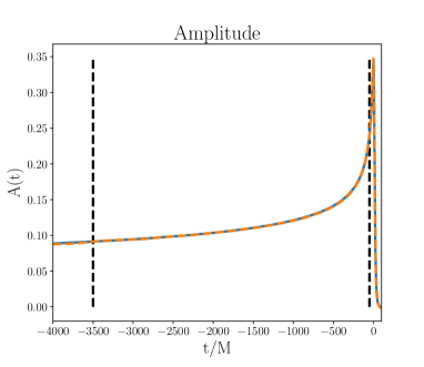
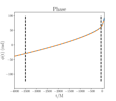
Figure 1: The key quantities of the GW signal of a precessing BBH, here illustrated for a binary with $(q,\chi_{1x},\chi_{1y},\chi_{1z},\chi_{2x},\chi_{2y},\chi_{2z})=(1.99,0.51,0.04,0.03,0.01,0.6,0.1)$. Left: the dimensionless amplitude $A(t)$. Right: the phase $\phi(t)$ (in unit radian). The black dashed lines show the points in time-space, where we perform different interpolation methods (t=-3500M and t=-50M).

We consider the following waveform training datasets in this study: (i) Three-dimensional datasets: Several interpolation methods we consider in this study require data on a regular grid. We prepare three-dimensional datasets $(q,\chi_{1z},\chi_{2z})$ in the mass-ratio $q=m_{1}/m_{2}$ and the aligned component spins $\chi_{iz}=\vec{S}_{i}\cdot\hat{L}_{N}/m_{i}^{2}$ for $i=1,2$. We do not include the total mass since it can be factored out from the waveform for GWs emitted from BBHs which are solutions of Einstein’s equations in vacuum. The grids have an equal number of points per dimension, ranging from 5 to 11. We choose parameter ranges $1\leq q\leq 10$ and $|\chi_{iz}|\leq 1$. (ii) The full intrinsic parameter space we consider is seven-dimensional: we include the dimensionless spin vector of each black hole $\chi_{i}=S_{i}/m_{i}^{2}$ and the mass-ratio $q$ of the binary. Due to the curse of dimensionality regular grid methods require a prohibitive amount of data in 7D. For instance, ten points per dimension would require $10^{7}$ waveform evaluations. Therefore, we only produce scattered waveform data in seven dimensions which are drawn from a random uniform distribution in each parameter. Here we choose parameter ranges $1\leq q\leq 2$ and $-1/\sqrt{3}\leq\vec{\chi}_{i}\leq 1/\sqrt{3}$. For both choices of dimensionality we also generate test data of 2500 points drawn randomly from the respective parameter space.

Waveform data in three and seven dimensions is produced at a total mass of $M=50M_{\odot}$ with a starting frequency of $20\mathrm{Hz}$. We align the waveform and frames at $t_{\mathrm{align}}=-2000M$ with the above procedure. We record waveform data from the key quantities at two different times, $t_{\mathrm{target}}=-3500M$ and $-50M$, where we have performed alignment in time such that the mode sum of the waveform amplitudes peaks at $t=0M$. This choice allows us to independently probe the inspiral and the merger regime. We expect that the waveform data will be very smooth in the inspiral, but more irregular close to merger due to the calibration of internal model parameters to numerical relativity waveforms at a limited number of points in parameter space.

2.2 Regression methods: a general overview

A large number of techniques have been developed to improve the speed and accuracy of generating gravitational waveforms. A priori, one would expect that higher speed would go hand-in-hand with less accuracy and less complexity. One frequent question is how to select a method for a specific purpose. Depending on the goals, a choice needs to be made between complex, highly accurate methods with moderate efficiency versus simpler but more efficient methods, and we can choose to trade accuracy for speed.

In this subsection, we discuss various methods and categorize them into two groups. The first group is comprised of traditional interpolation and fitting methods which are based on mathematical techniques and algorithms that are straightforward to implement and easily evaluated. The second group is made up of machine-learning (ML) methods which may require a more advanced mathematical and computational background. Methods from the second group are in general more complex and require more computational resources than the first group. Here we give a basic description of these methods, their limitation and provide some references.

2.2.1 Traditional interpolation and fitting methods

The traditional interpolation and fitting methods are either interpolatory, i.e., the approximation is designed such that it exactly includes the data points, or they produce an approximate fit, where a distance function between the data and the model is minimized. Many of these methods rely on polynomials as building blocks to model the data. Some models have a fixed order of approximation, while others let the number of terms be a free parameter. These methods are relatively straightforward to use and do not usually require much computational power.

1. Linear interpolation

   Linear interpolation is a straight line approximation that predicts the value of an unknown data point which lies between two known points [50]. Given its simplicity, this method has been widely used as a standard method to perform interpolation in various fields. If we have several data points, the transition between the adjacent data points is only continuous but not smooth. Higher order methods such as cubic interpolation can be used if a smoother approximation is desired (see subsection 2).

   Since linear interpolation is available as a standard Python package, we include this method to compare to other more complicated techniques. In particular, we investigate the application of multivariate linear interpolation on a regular grid using the regular grid interpolator (RGI) [51, 52] that is available in scipy.

   The mathematical background of linear interpolation can be explained as follows. Assume two known points $(x_{0},y_{0})$ and $(x_{1},y_{1})$ and an unknown point $(x,y)$ with $x_{0}\leq x\leq x_{1}$. This method assumes that the slope between $x_{0}$ and $x$ is equal to the slope between $x$ and $x_{1}$. Hence, we use the following relation to predict the data point $y$ in one dimension.

   $$\eqalign{\frac{y-y_{0}}{x-x_{0}}=\frac{y_{1}-y}{x_{1}-x}\cr\Leftrightarrow y=y_{0}+(x-x_{0})\frac{y_{1}-y_{0}}{x_{1}-x_{0}}.}$$ (7)

   In dimensions $d>1$, this method requires a regular grid of data points as a training set.

   Multivariate linear interpolation works as follows. Let $y_{i}(\vec{x})$ be the data point we want to predict, where $\vec{x}$ denotes the input parameters in $d$ dimensions. Initially, we need to obtain the parameters of the projection of $y_{i}(\vec{x})$ in $d-1$ dimensions, followed iteratively by $d-2$ and so on until we reach one-dimensional case $d=1$. Once we obtain these projection points, we can employ Eq (7) to predict the values of these points in one dimension. Subsequently, we use the predicted values as the known points to predict the result in higher dimensions iteratively. We then repeat the process further to find $y_{i}(\vec{x})$ in $d$ dimensions. This algorithm involves a small number of multiplications and additions, which are relatively fast.

   Since RGI assumes a regular grid, it is affected by the curse of dimensionality: the number of training points grows as the power of $d$. Therefore, we only investigate this method in three dimensions.

   Other popular regression methods that we do not consider here are ridge regression [53], LASSO regression [54], and Bayesian regression [55]. One reason is that the GW training data is quite well-behaved and does not usually include outliers such that would require special treatment.

2. Tensor product interpolation

   On regular or Cartesian product grids one can use the same univariate interpolation method in each dimension and the grid points can be unequally spaced. This gives rise to TPI methods. Popular choices for the univariate method are splines [56] and, if the data is very smooth, spectral interpolation [57, 58].

   Let us assume that we want to model a waveform quantity $X(t;\vec{\lambda})$ at a particular time $t=t_{\mathrm{i}}$. We define the $d$-dimensional TPI interpolant (where $d=\dim(\vec{\lambda})$) as an expansion in a tensor product of one-dimensional basis functions $\Psi_{j}(\lambda_{j})$,

   $$I[X](t_{\mathrm{i}};\vec{\lambda})=\sum_{j_{1},\dots,j_{d}}a_{j_{1},\dots,j_{d}}\left(\Psi_{j_{1}}\otimes\dots\otimes\Psi_{j_{d}}\right)(\vec{\lambda}),$$ (8)

   A popular choice for the basis functions are univariate splines, which are piecewise polynomials of degree $k-1$ (order $k$) with continuity conditions. For instance, cubic splines have degree $k=4$ and continuous first and second derivatives. The boundaries of the domain require special attention. A simple choice is the natural spline where the second derivative is set to zero at the endpoints. If boundary derivatives are not known it is better to use the so-called “not-a-knot” boundary condition [56]. This condition is defined by demanding that even the third derivative must be continuous at the first and last knots.

   To construct splines in a general manner it is advantageous to introduce basis functions with compact support, so-called B-splines. We denote the $i$-th B-spline basis function [56, 59] of order $k$ with the knots vector $\vec{t}$, a nondecreasing sequence of real numbers, evaluated at $x$ by $B_{i,k,t}(x)$. The knots refer to the locations in the independent variable where the polynomial pieces of B-spline basis function are connected. For distinct knots $t_{i},\dots,t_{i+k+1}$, the B-splines can be defined as

   $$B_{i,k,t}(x):=(t_{i+k}-t_{i})[t_{i},\dots,t_{i+k}](\cdot-x)_{+}^{k-1},$$ (9)

   where $[t_{i},\dots,t_{i+k}]f$ is the divided difference [56, 59] of order $k$ of the function $f$ at the sites $t_{i},\dots,t_{i+k}$, and $(x)_{+}:=\max\{x,0\}$. The B-splines can also be defined in terms of recurrence relations. The definition can be extended to partially coincident knots which are useful for the specification of boundary conditions. B-splines can be shown to form a basis [56] of the spline space for a given order and knots vector. A spline function or spline of degree $k$ with knots $\vec{t}$ can be then defined as an expansion

   $$s=\sum_{i}s_{i}B_{i,k,t}(x),$$ (10)

   with real coefficients $\{s_{i}\}_{i=1}^{n}$. Given data, a fixed order and knots vector, and a choice of boundary conditions, we can solve the linear system for the spline coefficients $s_{i}$. For efficient evaluation we only compute the parts of the B-spline basis functions that are nonzero.

   For smooth data, Chebyshev interpolation [57, 58] is a popular choice. Chebyshev polynomials (of the first kind) are defined as the unique polynomials satisfying

   $$T_{n}(\cos(\theta))=\cos(n\theta)$$ (11)

   on [-1,1]. In contrast to splines where the polynomial degree is usually low, global high order polynomial interpolation requires a special choice of nodes to be well-conditioned. A good choice are Chebyshev-Gauss-Lobatto nodes (which are defined to be the extrema of the $T_{n}(x)$ plus the endpoints of the domain)

   $$x_{k}=-\cos\left(\frac{k\pi}{m-1}\right),\quad k=0,\dots,m-1.$$ (12)

   Then we can approximate a function $f(x)$ by an expansion

   $$f(x)\approx I[f(x)]:=\sum_{k=0}^{m-1}c_{k}T_{k}(x),$$ (13)

   For $f\in C^{\infty}$ the error of Chebyshev interpolation converges exponentially with the number of polynomials $T_{n}(x)$.

   Tensor product interpolation is a very useful tool for constructing fast reduced order models (ROM) or surrogate models of time or frequency dependent functions that depend on a moderate number of parameters $\vec{\lambda}$. TPI with splines and Chebyshev polynomials has been used to build several GW models [21, 29, 24, 23] and [60], respectively. TPI is not available in standard Python packages. For TPI spline interpolation we use the Cython [61] implementation in the TPI package [62].

3. Polynomial fits

   A polynomial fit is a multiple linear regression model where the independent variables form a polynomial [63]. Different settings of maximum polynomial degrees may cause underfitting or overfitting, therefore care must be taken in choosing the ansatz.

   Assume that we have $N$ training points $(\{\vec{x}_{i},y_{i}\}\in\mathbb{R}^{d}\times\mathbb{R}|i=1,\cdots,N)$. Our goal is to find a function or regressor such that each $\vec{x}_{i}$ yields an output with the lowest error against its function values $y_{i}$. We assume that this function $f(\vec{x})$ is expressed by a polynomial of degree $k$ and parameters $\vec{c}$.

   In one dimension we have:

   $$f(\vec{x})=c_{0}x^{k}+c_{1}x^{k-1}+\cdots+c_{k-1}x+c_{k}.$$ (14)

   If we had as many degree of freedom as data points, we could demand:

   $$f(x_{i})=y_{i}.$$ (15)

   In matrix form, Eq (15) can be written as:

   $$\mathbf{X}\vec{c}=\vec{Y}$$

   $$\left({\begin{array}[]{ccccc}x_{1}^{k}&x_{1}^{k-1}&\cdots&x_{1}&1\\ x_{2}^{k}&x_{2}^{k-1}&\cdots&x_{2}&1\\ \vdots&&\ddots&&\vdots\\ x_{N}^{k}&x_{N}^{k-1}&\cdots&x_{N}&1\\ \end{array}}\right)\left(\begin{array}[]{c}c_{0}\\ c_{1}\\ \vdots\\ c_{k}\end{array}\right)=\left(\begin{array}[]{c}y_{1}\\ y_{2}\\ \vdots\\ y_{N}\end{array}\right),$$ (28)

   where X is the $N\times(k+1)$ Vandermonde matrix. The parameters $\vec{c}$ are obtained by solving Eq (3) for the known input and output data, X and $\vec{Y}$ in the training set. In general, the linear system may be over or under determined such that no unique solution would exist. Instead, we employ the standard discrete least squares fit to minimize the error (see section 10 of [64] and [65]):

   $$\Sigma_{j=1}^{N}|{f(x_{j})-y_{j}}|^{2}$$ (29)

   Similar to linear interpolation, univariate polynomial interpolation is available in the scipy package.

   Ref [63] discusses several methods and provide an overview of multivariate interpolation with polynomials. We employ polynomial fits for multivariate interpolation as in [66] and explained more detail in [67].

4. Greedy multivariate polynomial fit (GMVP)

   London and Fauchon-Jones [31] recently introduced methods that build an interpolant for a given data set by adaptively choosing a small set of analytical basis function from a certain class of functions. In our study here, we test the GMVP procedure described in detail in Sec. II B of [31].

   In this method, a scalar function, $f$, that is known at discrete points in the $d$-dimensional parameter space, $\vec{x}_{j}=\{x^{1}_{j},x^{2}_{j},\ldots,x^{d}_{j}\}$, is approximated by a linear sum of analytical basis functions, $\phi_{k}(\vec{x})$,

   $$f(\vec{x})\approx\sum_{k}\mu_{k}\,\phi_{k}(\vec{x}).$$ (30)

   Given a set of basis functions, the coefficients $\mu_{k}$ are determined by a ‘least-squares’ optimal fit to the known function values $f(\vec{x}_{j})$. In practice, this is calculated using the pseudoinverse (Moore-Penrose) matrix of $\phi_{k}(\vec{x}_{j})$ (that is, the values of the basis functions at the given location in the parameter space).

   In GMVP, the basis functions are chosen to be multivariate polynomials of maximal degree $D$. In order to prevent overfitting, however, not all possible polynomial terms from the set

   $$\phi_{k}(\vec{x})\in\left\{\big{(}x^{1}\big{)}^{\alpha_{1}}\,\big{(}x^{2}\big{)}^{\alpha_{2}}\ldots\big{(}x^{n}\big{)}^{\alpha_{d}},\quad\sum_{i=1}^{n}\alpha_{i}\leq D\right\}$$ (31)

   are included in the basis. Instead, a greedy algorithm [67] iteratively adds the basis functions to (30) that minimize the error

   $$\epsilon^{2}=\frac{\sum_{j}\left[f(\vec{x}_{j})-\sum_{k}\mu_{k}\,\phi_{k}(\vec{x}_{j})\right]^{2}}{\sum_{j}\left[f(\vec{x}_{j})\right]^{2}}.$$ (32)

   This process terminates when the difference in $\epsilon$ between two successive iterations becomes smaller than some user-defined tolerance. In order to improve the stability of the algorithm, the maximally allowed multinomial degree $D$ is successively increased, which the authors of [31] refer to as degree tempering.

   In our study, we use GMVP with a tolerance of $\epsilon=5\times 10^{-4}$ and a maximal multinomial degree of $D=16$.

5. Radial basis functions (RBF)

   Radial basis functions [68] are an approximation for continuous functions, where the predicted outputs depend on the Euclidean distance between the points and a chosen origin. This method is applicable in arbitrary dimensions and does not require a regular grid.

   We include RBF in this study due to several reasons. Primarily, because this method is simple, rapid, and has been integrated as a standard Python package in scipy. Moreover, RBFs are used in machine learning as activation functions in radial basis functions neural networks (see section 2.2.2).

   The mathematical background of RBFs is explained as follows. Let $N$ be the number of training points, $\vec{x}_{i}$ the parameters of each data point, and $y_{i}$ the data defining the training set $\{(\vec{x}_{i},y_{i})\in\mathbb{R}^{d}\times\mathbb{R}|i=1,\ldots,N\}$.

   The goal is to find an approximant $s:\mathbb{R}^{d}\to\mathbb{R}$ to the function $y:\mathbb{R}^{d}\to\mathbb{R}$ such that $s(\vec{x}_{i})=y_{i}$ ($s$ interpolates $y$ at the chosen points) with the form:

   $$s(\vec{x})=\sum_{i=1}^{N}w_{i}\varphi(r),$$ (33)

   where $\vec{x}$ is the vector of independent variables, $w_{i}$ are the coefficients, $r$ is the Euclidean distance between $\vec{x}$ and $\vec{x}_{i}$ ($r=\|\vec{x}-\vec{x_{i}}\|$), and $\varphi(r)$ is known as the radial basis function.

   To obtain the approximant $s$, we need to solve:

   $$\Phi(r)\vec{w}=\vec{Y},$$ (34)

   where $\Phi(r)=\{\|\vec{x}-\vec{x_{i}}\|\}_{x,x_{i}\in\Xi}$, $\vec{Y}=\{y_{i}\}_{i=1}^{N}$ and $\vec{w}=\{w_{i}\}_{i=1}^{N}$. $\Xi$ is a finite subset of $\mathbb{R}^{d}$ with more than one element [68]. We can solve the linear system for the coefficients and obtain the interpolant. Hence, the computational complexity and thus the training time of RBF is dominated by the computation of vector coefficients $\vec{w}$ that involves matrix inversion and goes as $\mathcal{O}(N^{3})$ [69].

   The interpolation matrix $\Phi(r)$ has to be nonsingular so that it does not violate the Mairhuber-Curtis theorem [68]. The solution is to choose a kernel function such that $\Phi(r)$ is a semi-definite matrix and therefore nonsingular. One common choice is the multiquadric kernel function $\varphi(r)$ expressed by:

   $$\varphi(r)=\sqrt{1+\bigg{(}\frac{r}{\varepsilon}\bigg{)}^{2}},$$ (35)

   where $\varepsilon$ is the average distance between nodes based on a bounding hypercube as defined in scipy [70].

   The multiquadric kernel function is commonly applied to scattered data because of its versatility due to its adjustable parameter $\varepsilon$ which can improve the accuracy or the stability of the approximation. Ref. [68] shows that this kernel is also able to approximate smooth functions well so that it useful for approximation. Hence, we employ the multiquadric kernel function in this study.

2.2.2 Machine learning methods (ML)

Machine learning is the scientific study of computer algorithms and statistics which aims to find patterns or regularities in the data sets. Systems learn from the training data and can predict output values for test data. ML is a branch of artificial intelligence.

Although the distinction is a blur, one major difference between ML and traditional interpolation methods lies in their objectives. In traditional methods, the objective is not only to provide an approximation of an underlying function from which the training data were generated, but also to understand the mathematical process behind the relation of input and output data. In that case, we seek interpolants or fits which often can be found analytically by solving linear systems for the coefficients in the model. Hence, the traditional methods originated from approximation theory and numerical analysis in mathematics. Conversely, in machine learning, the objective is to recognize patterns from the input-output training set and to construct a model from this data. Although we know that the result follows some mathematical procedures that depend on free parameters, these details are considered to be less important. Hence ML can be seen as a sub-field of computer science.

1. Gaussian process regression (GPR)

   GPR is a unique method that combines statistical techniques and machine learning. It can predict function values away from training points and can provide uncertainties of the predicted values, which will be useful for certain applications. GPR can be used with multivariate scattered data.

   Compared to traditional methods, GPR requires more knowledge of advanced statistics such as covariance matrices, regression and Bayesian statistics for the optimization strategy. GPR can be considered as a combination of traditional and machine learning methods.

   We provide a summary of GPR as discussed in detail in Ref. [71, 72]. We start with the most important assumption in GPR. Any discrete set of function values $y_{i}=y(\vec{x_{i}})$ is assumed to be a realization of a Gaussian process (GP). Assuming the data can be pre-processed to have zero mean, $\mu(\vec{x})=0$, the covariance function $k(\vec{x},\vec{x}^{\prime})$ fully defines the Gaussian process:

   $$y(\vec{x})\sim GP\bigg{(}\mu(\vec{x})=0,k(\vec{x},\vec{x}^{\prime})\bigg{)}.$$ (36)

   Assume that we want to predict the value $y_{*}$ at $\vec{x}_{*}\in\mathbb{R}^{d}$ and that we have $N$ numbers of training points, where each point depends on $d$ parameters expressed by $\{(\vec{x}_{i},y_{i})|i=1,\ldots,N\}$. The training and test outputs can be written as follows:

   $$\left[{\begin{array}[]{c}\vec{y}\\ y_{*}\end{array}}\right]\sim\mathcal{N}\left(0,\left[{\begin{array}[]{cc}K(X,X)+\sigma_{n}^{2}I&K(X,X_{*})\\ K(X_{*},X)&K(X_{*},X_{*})\end{array}}\right]\right),$$ (37)

   where $K(X,X)$ denotes the matrix of the covariances evaluated at all pairs of the training points and similarly for $K(X_{*},X_{*})$, $K(X,X_{*})$, and $K(X_{*},X)$, $\sigma_{n}^{2}$ (also called nugget) is the variance of the Gaussian (white) noise kernel that will be discussed later (see the hyperparameters).

   Explicitly, in order to predict a single value $y_{*}$, we need to compute $K(X,X)$ as the covariance matrix between each point in the training set, $K(X,X_{*})$ and its transpose that are vectors and the scalar $K(X_{*},X_{*})$. In a different form, our main goal is to find the conditional probability expressed by the following distribution:

   $$p(y_{*}|\vec{x}_{i},\vec{x}_{*},\vec{y},\vec{\theta})=\mathcal{N}(\bar{y}_{*},\textrm{var}(y_{*})),$$ (38)

   i.e., the probability of finding the value $y_{*}$ given the training data $\vec{x}_{i}$ and $\vec{y}$, the hyperparameters $\vec{\theta}$, and the location $\vec{x}_{*}$ is a normal distribution with mean $\bar{y}_{*}$ and variance $\textrm{var}(y_{*})$.

   The mean and variance can be shown to be:

   $$\bar{y}_{*}=K(X_{*},X)(K(X,X))^{-1}_{ij}y_{j}$$ (39)

   $$\mathrm{var}(y_{*})=K(X_{*},X_{*})-K(X_{*},X_{i})(K(X,X))^{-1}_{ij}K(X_{*},X_{j}).$$ (40)

   In the equation above, the covariance $K(x_{i},x_{j})$ is expressed by:

   $$K(x_{i},x_{j})=\sigma_{f}^{2}k(x_{i},x_{j})+\sigma_{n}^{2}\delta_{ij},$$ (41)

   where $\sigma_{f}$ and $\sigma_{n}$ are hyperparameters, $\delta_{ij}$ is the standard Kronecker delta, $k(x_{i},x_{j})=k(r)$, and $r$ is the distance:

   $$r=\sqrt{(\vec{x}-\vec{x}^{\prime})^{T}M(\vec{x}-\vec{x}^{\prime})}.$$ (42)

   In the following, we discuss the form of $M$ as a diagonal matrix with a tunable length scale in each physical parameter which form part of the hyperparameters.
   

   The hyperparameters

   We assume that our training data has some numerical noise $\sigma_{n}^{2}$ and a scale factor $\sigma_{f}$ that can be estimated by optimizing the hyperparameters $\vec{\theta}=\{\sigma_{f},\sigma_{n},M\}$. For instance, the explicit form of $M$ in the seven-dimensional case is:

   $$M=\textrm{diag}(\ell_{q}^{-2},\ell_{\chi_{1x}}^{-2},\ell_{\chi_{1y}}^{-2},\ell_{\chi_{1z}}^{-2},\ell_{\chi_{2x}}^{-2},\ell_{\chi_{2y}}^{-2},\ell_{\chi_{2z}}^{-2}),$$ (43)

   where the $\ell_{i}$ are length scales. Ref. [73] describes the length-scale $\ell$ as the distance taken in the input space before the function value changes significantly. Small values of the lengthscale $\ell$ imply that the function values change quickly and vice versa. Hence, the lengthscale $\ell$ describes the smoothness of a function.

   To determine the hyperparameters, we can maximizse the marginal log-likelihood:

   $$\ln p(y_{i}|\vec{x}_{i},\vec{\theta})=-\frac{1}{2}\bigg{(}y_{i}(K(X,X))^{-1}_{ij}y_{j}+\ln|K(X,X)|+N\ln 2\pi\bigg{)}.$$ (44)

   Because the log-likelihood may have more than one local optimum, we repeatedly start the optimizer and we choose ten repetitions. For the first run, we set the initial value of each length scale to unity, with bounds of $10^{-5}$ to $10^{5}$. Furthermore, we set $\sigma_{n}^{2}=10^{-10}$, where higher $\sigma_{n}^{2}$ value means that the data are more irregular. The subsequent runs use the allowed values of the hyperparameters from the previous runs until the maximum number of iterations is achieved.

   In Eq (44), we see that the partial derivatives of the maximum log likelihood can be computed using matrix multiplication. However, the time needed for this computation grows with more data in the training set as $\mathcal{O}(N^{3})$. Additionally, we employ Algorithm 2.1 of [71], because Cholesky decomposition is about six time faster than the ordinary matrix inversion to compute Eq (44). We highlight that although GPR becomes more accurate in predicting the underlying functional form of the data given more training points $N$, it has complexity $\mathcal{O}(N^{3})$ and therefore the method becomes ineffective for large $N$.

   We estimate the posterior distribution of the hyperparameters using Bayes’ theorem as follows:

   $$p(\vec{\theta}|\vec{x}_{i},y_{i})\propto p(\theta)p(y_{i}|\vec{x}_{i},\vec{\theta}),$$ (45)

   where we employ a uniform prior distribution $p(\theta)$. Additionally, we use the sckit-learn package [72] to optimize the hyperparameters as in the implementation of Algorithm 2.1 in [71].

   This method is non-parametric because no direct model ansatz is used. Note however that a choice for the covariance function needs to be made.
   

   The covariance functions

   In statistics, covariance expresses how likely two random variables change together [74]. Various choices of covariance functions which are usually called kernels $k(\vec{x},\vec{x}^{\prime})$ are discussed in more detail in Ref. [72] and [71]. In this study, we compare the two most commonly used kernel functions in GPR: the squared exponential kernel and the Matérn kernel explained below.

   1. The squared exponential kernel (SE) is a standard kernel for Gaussian processes:

      $$k_{SE}(r)=\exp\bigg{(}\frac{-r^{2}}{\ell^{2}}\bigg{)},$$ (46)

      with $r$ defined in Eq. 42 and $\ell$ is the length-scale.

   2. The Matérn class of kernels is named after a Swedish statistician, Bertil Matérn and has less smoothness than the SE kernel. The Matérn kernel is given by:

      $$k_{M}(r)=\frac{2^{1-\nu}}{\Gamma(\nu)}\bigg{(}\frac{\sqrt{2\nu}r}{\ell}\bigg{)}^{\nu}K_{\nu}\bigg{(}\frac{\sqrt{2\nu}r}{\ell}\bigg{)},$$ (47)

      where $K_{\nu}$ is a modified Bessel function [75], $\Gamma$ is the gamma function and $\nu$ is usually half-integer. Common choices of $\nu$ are $k_{\nu=3/2}$ and $k_{\nu=5/2}$.

      $$k_{\nu=3/2}(r)=\bigg{(}1+\frac{\sqrt{3}r}{\ell}\bigg{)}\exp\bigg{(}-\frac{\sqrt{3}r}{\ell}\bigg{)},$$ (48)

      $$k_{\nu=5/2}(r)=\bigg{(}1+\frac{\sqrt{5}r}{\ell}+\frac{5r^{2}}{3\ell^{2}}\bigg{)}\exp\bigg{(}-\frac{\sqrt{5}r}{\ell}\bigg{)}.$$ (49)

      The Matérn kernel is a generalization of the radial basis function kernel. For $\nu=1/2$, it reduces to exponential kernel and $\nu=\infty$ reduces to the SE kernel. We use the Matérn kernel with $\nu=3/2$ in our analysis.

2. Artificial neural networks

   Artificial neural networks (ANNs) as computing systems are inspired by emulating the work of brains to learn complex things and to find patterns in biology. In machine learning algorithms, ANN has been widely used as a framework to perform advanced tasks such as pattern recognition [76], forecasting [77], and many other applications in various disciplines [78]. This framework works analogously to brains: it receives some inputs, processes them, and yields some output [79].

   In this study, we employ ANNs or feedforward networks as the simplest neural networks architecture to perform interpolation. The feedforward network with hidden layers can approximate of any function which is known as the universal approximation theorem [79, 80]. This class is called feedforward because the information flow from the input to the output and the connection between them does not form a cycle (loop). In our case, the inputs are the waveform’s parameters $\vec{\lambda}$ and the output is the predicted value of $A(t_{i};\vec{\lambda})$ or $\phi(t_{i};\vec{\lambda})$. We define hidden layer as a layer between the input and the output of ANN .

   Four types of commonly used ANNs are:

   • Single-layer perceptron
     In a single-layer perceptron, the inputs are weighted and fed directly to the output. Hence, the single-layer perceptron is the simplest neural network system.

   • Multi-layer perceptron
     In multi-layer-perceptron (MLP), there is at least one hidden layer between the input and the output layer, where each neuron in each layer is connected to another neuron in the following layer.

   • Radial basis function network
     This class has the same workflow and architecture as the MLP with input, hidden layers and output, where each neuron is connected directly to the following layer. The only difference is the input, where the radial basis function network (RBFN) uses the Euclidean distances with respect to some origin as its input and Gaussian activation functions [81].

   • Convolutional neural network
     The feedforward convolutional neural network is commonly used to train neural network for visual analysis. Convolutional neural networks use convolution in place of general matrix multiplication in at least one of its layers [79].

   We employ MLP as one of the simplest architectures to perform function approximation [80, 82]. Fig. 2 shows the illustration of the network architecture used in this study.

   

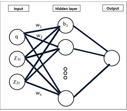
   Figure 2: Diagram of ANN architecture used for three-dimensional interpolation in this study. The circles represent the neurons and we indicate weigths $w_{i}$ along neuron connections and biases $b_{i}$.We employ two layers in the hidden layer part of the diagram. The same architecture is used for the seven-dimensional case, where the input contains seven neurons that depend on the seven parameters.

   In Fig. 2, each layer consists of a finite number of neurons. Each neuron in each layer is connected to the subsequent layer and the previous layer which are generally called links or synapses. The workflow of MLP is explained as follows:

   1. Define the input as $x_{ij}$, where $i$ is the index of the layers. Starting at $i=0$ at the input layer, and $j$ indexes the neurons in a layer. Thus, with $x_{0j}$, $j=1,2,3$ corresponds to $q,\chi_{1z},\chi_{2z}$ respectively.

   2. The $k$-th neuron of the $({i+1})$-th layer receives the value of $x_{ij}$ from the ${i}$-th layer multiplied by the weight $w_{ijk}$. These products are then summed over all links from the $i$-th to the $(i+1)$-th layer.

   3. A bias or shift $b_{ik}$ is added to the above value and an activation function $\sigma$ is applied to the final result. In this study, we use the Rectified Linear Unit (ReLU) [83] because it faster than other functions such as sigmoid and tanh and it is commonly used in other studies. ReLU is mathematically expressed by the following equation:

      $$\sigma(z)=\textrm{max}(z,0),$$ (50)

   and the MLP procedure is expressed by the following relation:

   $$x_{i+1,k}=\sigma\left(\sum_{j}w_{ijk}x_{ij}+b_{ik}\right)$$ (51)

   We vary the number of neurons in the first hidden layer between 2 to 2000 for the three-dimensional data sets and 2 to 5000 for the seven-dimensional data sets. We then set the number of neurons in the second hidden layer identical to the first hidden layer. For each network and training data set, we compute mean squared error and the mean absolute error (see [84]) of $A(t)$ and $\phi(t)$, respectively.

   To train the networks, the training data is separated into several batches, where each batch contains the same number of data samples. Each batch is then passed through the networks (see Eq. 51). When each data sample in the training set has had an opportunity to pass the networks a single time, this is known as an epoch. The number of epochs affects the learning of the networks, i.e., the higher the epoch, the better the learning. In this study, we set our batch size to five and train them through one thousand epochs.

   The networks compute the loss functions during each epoch. The loss functions measure the errors or inconsistency between the predicted value and the true data. In this study, we employ the mean squared error loss function for $A(t)$ and the absolute error for $\phi(t)$ respectively (see Ref. [84]).

   Training neural networks means that we minimize the loss functions so that our predicted values are as close as possible to the true values [85]. To minimize the loss functions, the networks adjust learnable parameters, i.e., the values of the weights and biases of the model. In most cases, the minimization cannot be solved analytically, but can be approached with optimization algorithms.

   During optimization, the network learns the values of weights and biases of the previous epoch and calculates its loss functions. Subsequently, it adjusts the values of weights and biases in the next epoch so that the loss functions become smaller. One way to minimize the loss functions is to compute the gradient values with respect to the learnable parameters. In this study, we employ Adam [86] as the optimization algorithm. Adam is a popular algorithm in deep learning due its robustness (see Ref. [86] for more detail).

   Following the above procedure, a model is then saved at the end of the run and evaluated through the test data. We then compute the accuracy and execution time of this process similar to other methods. We employ Keras [84] and TensorFlow [87] to perform this computation.

3 Results

In this section, we show results for accuracy and computational time for different regression methods. We apply methods to the three-dimensional and seven-dimensional data sets defined in sec. 2.2.

3.1 Three-dimensional case

We investigated the results for aligned spin waveforms with parameters $q,\chi_{1z}$, and $\chi_{2z}$. Training points were given on a regular grid. We placed the same number of points equally spaced to each other for each parameter (see sec. 2.1). Hence the total number of training points is proportional to the number of training points per dimension cubed. We then varied the number of training points in each dimension from five to eleven which corresponds to a total number of training points of 125 to 1331. We distributed 2500 test points randomly (see section 2.1). These test points are located inside the same domain covered by the training points. Hence, we do not test how well the methods perform for extrapolation.

We calculated relative errors (in percent) for the amplitude $A(t)$:

$$\varepsilon_{re}=\frac{\sum_{i}^{N}|A_{\mathrm{pred}}^{i}(t)-A_{\mathrm{true}}^{i}(t)|}{\sum_{i}^{N}|A_{\mathrm{true}}^{i}(t)|}\times 100.$$ (52)

The phase error is an important diagnostic to measure the accuracy of GW waveform models. Therefore, we consider the absolute phase error (in radians)

$$\varepsilon_{ae}=\frac{1}{N}\sum_{i}^{N}|\phi_{\mathrm{pred}}^{i}(t)-\phi_{\mathrm{true}}^{i}(t)|.$$ (53)

$\varepsilon_{re}$ and $\varepsilon_{ae}$ are the relative error and the average of the absolute error, respectively, $A_{\mathrm{pred}}(t)$ and $\phi_{\mathrm{pred}}(t)$ are the predicted results of the amplitude and phase regression respectively, and $A_{\mathrm{true}}(t)$ and $\phi_{\mathrm{true}}(t)$ are their true values.

Subsequently, we investigated the computational time taken to evaluate each interpolation method. Here we define the training time as the time to compute the interpolant and the execution time being the time to compute the 2500 interpolation points following our test set. Furthermore, we define total time as the sum between the training time and the execution time, i.e., the entire process to perform interpolation for 2500 points. The comparison results in the early inspiral ($t=-3500M$) are shown in Fig. 3, whereas the results at $t=-50M$ are shown in Fig. 4. We now discuss the results shown the results for different regression methods.

1. Traditional interpolation and fitting methods & GPR

   We expect that the key quantities for two waveform models, SEOBNRv3 and IMRPhenomPv2 agree quite well in the early inspiral. The error in $A(t)$ and $\phi(t)$, decreases with more training points for both models. This result is expected as we populate our parameter space with more points located on a regular grid.

   For both quantities, we find that errors for different methods are similar between waveform models. GPR errors show a dependence on the kernel choice. We first consider the amplitude errors. For SEOBNRv3 the errors fall off in a similar way for either choice of kernel, whereas for IMRPhenomPv2 the error is much higher for the SE kernel compared to the Matérn kernel. This is likely due to the higher level of noise in the IMRPhenomPv2 data due to the inverse Fourier transformation.

   The SE kernel assumes a higher degree of smoothness in the data than the Matérn kernel. Similarly, we find for either waveform model that the SE kernel shows a higher phase error than the Matérn kernel.

2. Artificial neural networks

   We now discuss errors for ANNs as indicated by the filled circles in Fig. 3. Here we compare the results of the double layer MLP with various numbers of neurons. By design, the double layer MLP consists of one input layer, two hidden layers, and one output layer. We set the number of inputs as the dimensionality of the parameter space and only produce a single output. In the aligned spin case, our inputs are the parameters $q,\chi_{1z}$, and $\chi_{2z}$ and output is either $A(t)$ or $\phi(t)$. For the hidden layers, we varied the number of neurons between 2 and 2000 in the first hidden layer, and set an equal number of neurons for the second hidden layer.

   Thus, we obtained a set of errors as we modified the number of neurons in the hidden layers for a fixed number of training points $N$ per dimension. In Fig. 3, we only show the results of the smallest errors for each training set. In this plot, different colors of the circles correspond to different numbers of neurons as indicated by the color bar. We note that the ANN with the smallest error may not be the fastest one.

   Regarding the computational time, the training time obviously grows with the number of neurons per layer. However, we argue that there is no guarantee that many neurons yield smaller error than fewer neurons. In fact, too many neurons lead to overfitting and too few neurons lead to underfitting. We could reduce overfitting by activating the Dropout function in Keras, Dropout removes the result from a selected number of neurons randomly. However, we prefer to not include an additional stochastic element and do not include Dropout in this study.

   Next, we compare execution times. Execution time is relatively similar between the GPR, RBF, TPI, and ANN methods. Other traditional methods such as linear, polynomial fit and GMVP, and linear interpolation are faster.

   To ensure a fair comparison between all methods, we explored the performance on the same machines (2x Intel Xeon E5-2698 v4) with 20 CPU cores, 256 Gigabytes of RAM, and 1x HDD (1TB, 6Gbps) of storage.

   Due to the limited scope of our study, we only investigate results for the double layer ANN. This leaves tuning parameters and architectures to be explored in future studies. A possible way to reduce training and execution times is to use on GPUs instead of CPUs.

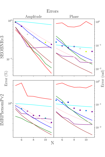
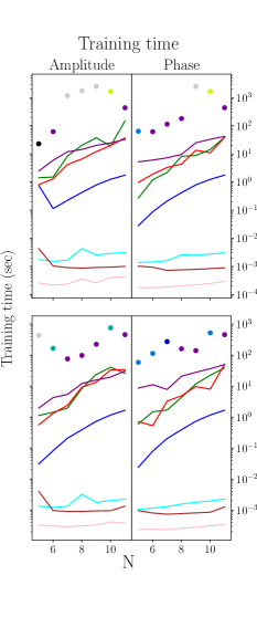
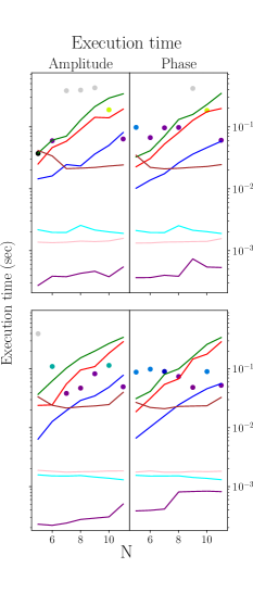
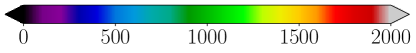
Figure 3: The three-dimensional interpolation results at t=-3500M. Top:SEOBNRv3, bottom:IMRPhenomPv2. The $x$-axes show the number of training points in each dimension, $N$, and the $y-$axes show the errors, training, and indicated execution time as on the labels of the panels. Left: errors of the amplitude and phase respectively, middle: training time in (seconds), and right: execution time (seconds). Different colors represent different interpolation methods as shown in the shared legend. The colored circles show ANN results, where different colors represent the number of neurons per layer in a double layer ANN as shown in the corresponding color bar.

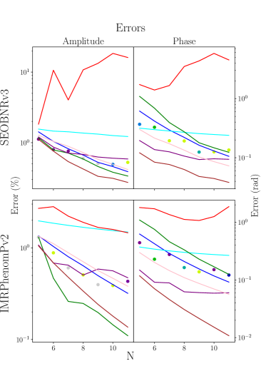
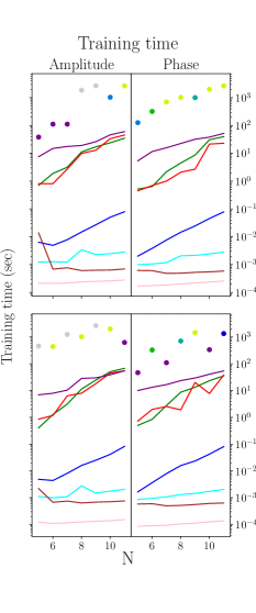
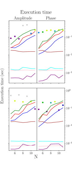
Figure 4: The three-dimensional interpolation results at t=-50M. Top:SEOBNRv3, bottom:IMRPhenomPv2. The $x$-axes show the number of training points in each dimension, $N$, and the $y-$axes show the errors, training, and indicated execution time as on the labels of the panels. Left: errors of the amplitude and phase respectively, middle: training time in (seconds), and right: execution time (seconds). Different colors represent different interpolation methods as shown in the shared legend. The colored circles show ANN results, where different colors represent the number of neurons per layer in a double layer ANN as shown in the corresponding color bar.

Finally, we discuss results for training times. The training time for RBF and GPR rise proportionally with the number of training points. In RBF, this is caused by the least-squares-fit computation that takes a longer time with more training points. For GPR, the training time goes as $\mathcal{O}(N^{3})$ with $N$ the number of training points as explained in Sect. 2.2. Polynomial fit, TPI and linear interpolation do not depend strongly on the size of the training set and their training time is relatively fast.

For both models, ANN yields comparable errors and execution times as other interpolation methods, but generally with longer training time than other methods. Several methods have execution times that are independent of the size of the training set for a fixed order of approximations. This includes TPI, linear interpolation, polynomial fit, and ANNs.

Combining all the results at $t=-3500M$ and at $t=-50M$, we found that the errors are generally larger in noisy data. We also found that the methods with longer training time do not always yield a better result than the methods with less training time (see Fig. 4).

Using too many neurons in the hidden layers may cause problems such as overfitting. It occurs when the networks have too much capacity to process information such that the amount of information in the training set is not enough to train the networks [88]. Hence, the number of neurons must be set such that there are not too few or not too many. The selection however, depend on the architecture of the networks and the hyperparameters.

3.2 Seven-dimensional case

In seven dimensions, we distribute the training points randomly in each dimension. The main reason for this placement is to avoid the curse of dimensionality as explained in the previous section. Similarly to the three-dimensional case, we investigate training sets of different sizes, from 500 to 3000 points. As discussed in Sec. 2.1, the seven-dimensional case has a narrower range of mass ratio ($1\leq q\leq 2$) than the three-dimensional one ($1\leq q\leq 10$) and full-spin range.

We construct a single test set with 2500 points distributed randomly and located within the parameter ranges. Some of the test points may be outside the domain covered by the training points. This means that our results may contain a small extrapolation.

Since TPI and linear interpolation require regular grid training points, we do not include them in our analysis. For other methods, we employed the same settings (kernels, hyperparameters, degree) as in the three-dimensional case.

We built the architecture of ANN in a similar way as before. The results of the seven-dimensional case for different interpolation methods ($t=-3500M$ and $t=-50M$) are shown in Fig. 5.

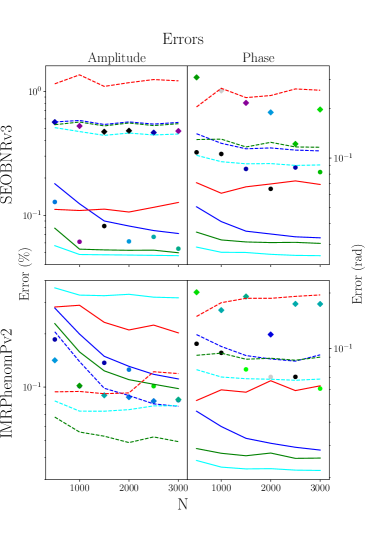
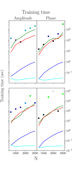
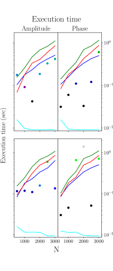
Figure 5: The seven-dimensional interpolation results. Top:SEOBNRv3, bottom:IMRPhenomPv2. The $x$-axes show the number of training points $N$ and the $y$-axes shows the errors, training, and execution time as shown on the plot. Left: errors of the amplitude ($A(t)$) and phase ($\phi(t)$) respectively, middle: training time in unit seconds, and right: execution time in unit seconds. The solid lines show the results at $t=-3500M$ and the dashed lines for $t=-50M$. Different colors represent different interpolation methods as shown in the shared legend. The colored circles correspond to the results of ANN at $t=-3500M$ and the colored diamonds for $t=-50M$. Different colors represent a different number of neurons on a double layer ANN as shown in the corresponding color bar.

We observed that errors of SEOBNRv3 are not significantly different than the corresponding three-dimensional results. Furthermore, the errors of this model at $t=-50M$ are higher than at $t=-3500M$ in a similar way as in three dimensions.

Surprisingly, the relative amplitude errors for IMRPhenomPv2 (top left plots) in the late inspiral are smaller than in the early inspiral in contrast to SEOBNRv3. The $A(t)$ quantity of IMRPhenomPv2 is smoother at $t=-50M$ than at $t=-3500M$. We emphasize that both models, SEOBNRv3 and IMRPhenomPv2 have comparable amplitude values at $t=-50M$ and at $t=-3500M$.

In the early inspiral ($t=-3500M$), both waveforms agree well, similar to the three-dimensional case. Hence, the percent errors are not significantly different as shown in the same plot.

The phase errors were computed as absolute errors (see Eq. 53). We find that the phase errors for SEOBNRv3 and IMRPhenomPv2 are comparable. Furthermore, the late inspiral errors are higher than the early inspiral as the data fluctuates more. In Fig. 5, we observe a similar behavior for the training time as in three dimensions, where higher training time was found for GPR, ANN, and RBF. This is caused by the same factors as explained in the three-dimensional case. For the execution time (right panel), we found that the more complex methods take longer time than the simpler methods. For RBF and GPR this is due to their dependence on the size of the training set. Interestingly, the execution time for ANNs is faster than GPR and RBF. This is because ANN picks the optimum weights and biases during the training and its execution time does not depend on the number of training points in the data.

We remind the reader that we set the parameter space of the seven-dimensions analysis narrower in mass ratio than the three-dimensions. Hence, the errors should not be compared directly to the three-dimensional case. For the same parameter ranges, the seven dimensional case yields errors up to 100 times larger for the $A(t)$ and 15 times larger for the $\phi(t)$. The order of accuracy does not significantly change, where the best accuracy in this range is obtained by polynomial interpolation.

Overall, we found that in some cases, a simple method such as polynomial fit yields lower errors and performs faster than the more complex methods.

4 Discussion and conclusion

Various approximation methods play important roles in building gravitational waveform models. Methods with high accuracy, low complexity, and fast computational time are needed for current and future applications. In this paper, we presented a comparative study of interpolation, fitting and regression methods applied to precessing and aligned BBH systems. Precessing BBH model depends on seven key intrinsic parameters ($q,\vec{\chi}_{1},\vec{\chi}_{2}$), whereas the aligned model depends on three parameters ($q,\chi_{1z},\chi_{2z}$).

We generated the data sets in the time domain using two waveform models: SEOBNRv3 (originally built in the time domain) and the inverse Fourier transform of IMRPhenomPv2 (originally built in frequency domain). The full waveforms were transformed into a precession adapted frame where we extracted two quantities: amplitude $A(t)$ and phase $\phi(t)$ as explained in section 2.1 to perform a comparative study. For each key quantity, we picked two points in time, $t=-3500M$ in the inspiral for the smoother data set and $t=-50M$ near merger for the more irregular data. We employed this procedure on different numbers of training sets and used different approximation methods.

We split approximation methods into two categories: traditional methods and machine learning mehods (see Sect. 2.2). The traditional methods consist of linear interpolation, polynomial fits, radial basis function, GMVP, and TPI. Since linear interpolation and TPI package require a regular grid, we do not include them in the seven dimensional analysis. Furthermore, we investigated machine learning methods such as GPR and ANN. For GPR, we compared two kernel functions: the square exponential kernel and the Matérn kernel. We took the mean results of each kernel and compared them against other methods. For ANN, we focused on networks with two hidden layers and varied the number of their neurons.

We computed the relative errors for $A(t)$ and the absolute errors for $\phi(t)$. To validate the result, we generated 2500 test points distributed randomly within the same parameter space. The comparison results of different methods in accuracy, training time and execution time (in second) are presented in Sec.3.

We found that all methods perform better with more training data. Furthermore, we compared the performance of the same method in a set of smoother data and a set of more irregular data. In general, we found that approximation methods perform better in smoother data as expected. We recommend to use preprocessing methods to improve the smoothness of the data where possible which should increase the accuracy of regression results. This preparation is crucial as any methods perform well with smoother data sets. Different accuracies are attained by different methods in handling the irregularities in the data. We give a brief summary of different methods in Table. 1.

Methods	Advantages	Disadvantages	Training
			time
Linear (RGI)	standard scipy	needs regular grid	$\mathcal{O}(N$)
TPI	robust and	needs regular grid	$\mathcal{O}(N^{k})$
	high accuracy
GMVP	irregular grid	complex	#basis function
	fast execution time		#error tolerance
Polynomial fit	irregular grid	Runge’s phenomenon	$\mathcal{O}(N)$ and
	simple and fast	only univariate in scipy	#polynomial degree
RBF	scipy	high computational	$\mathcal{O}(N^{3}$)
	irregular grid	complexity
GPR	irregular grid	depends on the choice	$\mathcal{O}(N^{3}$)
	can predict uncertainty	of kernel and hyperparameters
		complex
ANN	irregular grid	complex	#neurons
	flexible architecture choices		#hidden layers

Table 1: Summary of features of the methods used in this study. We present the advantages, the disadvantages and the scaling complexity for each method. For linear interpolation, TPI, RBF, and GPR the (training time) depends on the number of training points $N$ (and polynomial degree $k$). Other methods have different complexity scalings that affect their training time.

For lower dimensions, simpler methods such as linear interpolation and TPI provide good accuracy and speed. However, these methods need a regular grid and therefore are less useful for high dimensional data sets as explained above. For this situation, we found that polynomial fits are one of the simplest methods that offers a good combination between accuracy and speed. Furthermore, polynomial fits have been used widely and can be coded manually making it reliable and easy. The computational timing of polynomial fits depends on the number of parameters and the maximum polynomial degree. Another method that can perform approximation of scattered data sets is GMVP. GMVP which is based on polynomials can perform very well by setting error tolerance on its algorithm. For lower dimensionality, GMVP is computationally cheap. However, as the number of parameters rise, the computational time to compute the interpolant with the same error tolerance grows significantly higher. Therefore, we do not include this method in our analysis for the seven-dimensional case.

RBF and GPR are promising methods for scaterred data points. RBF has been integrated in a standard scipy package, making it easy for users. GPR computes the uncertainty of the predicted values. This feature is useful for future applications and cannot be found in other methods. Furthermore, GPR has been integrated in sckit-learn package [72]. Both RBF as GPR have the freedom to choose suitable kernel functions and hyperparameters. However, their speed depends on the number of training points cubed $\mathcal{O}(N^{3})$. Hence, these methods become inefficient for larger data set.

A simple ANN can be used to perform regression for scattered data points. Similar to GPR, this method is more complex and depends on the choice of architecture and hyperparameters. We showed that the the three-dimensional result of ANN requires a longer training time with relatively comparable accuracy to other methods. We argue that such complexity is less needed for lower dimensional parameter and users should use a more simpler methods that provide good accuracy and speed. However, ANN is highly versatile to solve problems in higher dimensions and is promising to be explored further.

One might expect that methods with higher complexity perform better than methods with lower complexity. We find that this is not always the case. A more complicated method does not guarantee that the results are always better or faster. We find that simpler methods may yield smaller errors than more complex methods and perform faster in many cases. Hence, we suggest that one should critically evaluate the performance of approximation methods and understand the features of the method that are necessary for the data of interest. Simpler methods that perform better or at least equal to more complicated methods should be used as the first choice to avoid unecessary complexity.

References

References

- [1] LIGO: The laser interferometry gravitational wave detector;. https://www.ligo.caltech.edu.
- [2] Virgo;. http://www.virgo-gw.eu.
- [3] Abbott BP, et al. GWTC-1: A Gravitational-Wave Transient Catalog of Compact Binary Mergers Observed by LIGO and Virgo during the First and Second Observing Runs. Phys Rev X. 2019 Sep;9:031040. Available from: https://link.aps.org/doi/10.1103/PhysRevX.9.031040.
- [4] LIGO third obesrerving time (O3);. https://dcc.ligo.org/public/0152/G1801056/004/G1801056-v4.pdf.
- [5] Blanchet L. Gravitational Radiation from Post-Newtonian Sources and Inspiralling Compact Binaries. Living Reviews in Relativity. 2014 Feb;17. Available from: https://link.springer.com/article/10.12942/lrr-2014-2#aboutcontent.
- [6] Campanelli M, Lousto CO, Marronetti P, Zlochower Y. Accurate Evolutions of Orbiting Black-Hole Binaries without Excision. Phys Rev Lett. 2006 Mar;96:111101. Available from: https://link.aps.org/doi/10.1103/PhysRevLett.96.111101.
- [7] Pretorius F. Evolution of Binary Black-Hole Spacetimes. Phys Rev Lett. 2005 Sep;95:121101. Available from: https://link.aps.org/doi/10.1103/PhysRevLett.95.121101.
- [8] Baker JG, Centrella J, Choi DI, Koppitz M, van Meter J. Gravitational-Wave Extraction from an Inspiraling Configuration of Merging Black Holes. Phys Rev Lett. 2006 Mar;96:111102. Available from: https://link.aps.org/doi/10.1103/PhysRevLett.96.111102.
- [9] Damour T. Coalescence of two spinning black holes: An effective one-body approach. Phys Rev D. 2001 Nov;64:124013. Available from: https://link.aps.org/doi/10.1103/PhysRevD.64.124013.
- [10] Damour T, Jaranowski P, Schäfer G. Effective one body approach to the dynamics of two spinning black holes with next-to-leading order spin-orbit coupling. Phys Rev D. 2008 Jul;78:024009. Available from: https://link.aps.org/doi/10.1103/PhysRevD.78.024009.
- [11] Babak S, Taracchini A, Buonanno A. Validating the effective-one-body model of spinning, precessing binary black holes against numerical relativity. Phys Rev D. 2017 Jan;95:024010. Available from: https://link.aps.org/doi/10.1103/PhysRevD.95.024010.
- [12] Bohé A, et al. Improved effective-one-body model of spinning, nonprecessing binary black holes for the era of gravitational-wave astrophysics with advanced detectors. Phys Rev D. 2017 Feb;95:044028. Available from: https://link.aps.org/doi/10.1103/PhysRevD.95.044028.
- [13] Santamaría L, Ohme F, Ajith P, Brügmann B, Dorband N, Hannam M, et al. Matching post-Newtonian and numerical relativity waveforms: Systematic errors and a new phenomenological model for nonprecessing black hole binaries. Phys Rev D. 2010 Sep;82:064016. Available from: https://link.aps.org/doi/10.1103/PhysRevD.82.064016.
- [14] Khan S, Husa S, Hannam M, Ohme F, Pürrer M, Forteza XJ, et al. Frequency-domain gravitational waves from nonprecessing black-hole binaries. II. A phenomenological model for the advanced detector era. Phys Rev D. 2016 Feb;93:044007. Available from: https://link.aps.org/doi/10.1103/PhysRevD.93.044007.
- [15] Hannam M, Husa S, González JA, Sperhake U, Brügmann B. Where post-Newtonian and numerical-relativity waveforms meet. Phys Rev D. 2008 Feb;77:044020. Available from: https://link.aps.org/doi/10.1103/PhysRevD.77.044020.
- [16] Husa S, Khan S, Hannam M, Pürrer M, Ohme F, Forteza XJ, et al. Frequency-domain gravitational waves from nonprecessing black-hole binaries. I. New numerical waveforms and anatomy of the signal. Phys Rev D. 2016 Feb;93:044006. Available from: https://link.aps.org/doi/10.1103/PhysRevD.93.044006.
- [17] Schmidt P, Hannam M, Husa S. Towards models of gravitational waveforms from generic binaries: A simple approximate mapping between precessing and nonprecessing inspiral signals. Phys Rev D. 2012 Nov;86:104063. Available from: https://link.aps.org/doi/10.1103/PhysRevD.86.104063.
- [18] Hannam M, Schmidt P, Bohé A, Haegel L, Husa S, Ohme F, et al. Simple Model of Complete Precessing Black-Hole-Binary Gravitational Waveforms. Phys Rev Lett. 2014 Oct;113:151101. Available from: https://link.aps.org/doi/10.1103/PhysRevLett.113.151101.
- [19] Blackman J, Field SE, Galley CR, Szilágyi B, Scheel MA, Tiglio M, et al. Fast and Accurate Prediction of Numerical Relativity Waveforms from Binary Black Hole Coalescences Using Surrogate Models. Phys Rev Lett. 2015 Sep;115:121102. Available from: https://link.aps.org/doi/10.1103/PhysRevLett.115.121102.
- [20] Blackman J, et al. Numerical relativity waveform surrogate model for generically precessing binary black hole mergers. Phys Rev D. 2017 Jul;96:024058. Available from: https://link.aps.org/doi/10.1103/PhysRevD.96.024058.
- [21] Doctor Z, Farr B, Holz DE, Pürrer M. Statistical gravitational waveform models: What to simulate next? Phys Rev D. 2017 Dec;96:123011. Available from: https://link.aps.org/doi/10.1103/PhysRevD.96.123011.
- [22] Varma V, Field SE, Scheel MA, Blackman J, Kidder LE, Pfeiffer HP. Surrogate model of hybridized numerical relativity binary black hole waveforms. Phys Rev D. 2019 Mar;99:064045. Available from: https://link.aps.org/doi/10.1103/PhysRevD.99.064045.
- [23] Pürrer M. Frequency-domain reduced order models for gravitational waves from aligned-spin compact binaries. Classical and Quantum Gravity. 2014 September;31:195010. Available from: http://iopscience.iop.org/article/10.1088/0264-9381/31/19/195010/pdf.
- [24] Pürrer M. Frequency domain reduced order model of aligned-spin effective-one-body waveforms with generic mass ratios and spins. Phys Rev D. 2016 Mar;93:064041. Available from: https://link.aps.org/doi/10.1103/PhysRevD.93.064041.
- [25] Abbott BP, et al. GW150914: First results from the search for binary black hole coalescence with Advanced LIGO. Phys Rev D. 2016 Jun;93:122003. Available from: https://link.aps.org/doi/10.1103/PhysRevD.93.122003.
- [26] Veitch J, et al. Parameter estimation for compact binaries with ground-based gravitational-wave observations using the LALInference software library. Phys Rev D. 2015 Feb;91:042003. Available from: https://link.aps.org/doi/10.1103/PhysRevD.91.042003.
- [27] Veitch J, Mandel I, Aylott B, Farr B, Raymond V, Rodriguez C, et al. Estimating parameters of coalescing compact binaries with proposed advanced detector networks. Phys Rev D. 2012 May;85:104045. Available from: https://link.aps.org/doi/10.1103/PhysRevD.85.104045.
- [28] Field SE, Galley CR, Hesthaven JS, Kaye J, Tiglio M. Fast Prediction and Evaluation of Gravitational Waveforms Using Surrogate Models. Phys Rev X. 2014 Jul;4:031006. Available from: https://link.aps.org/doi/10.1103/PhysRevX.4.031006.
- [29] Blackman J, et al. A Surrogate model of gravitational waveforms from numerical relativity simulations of precessing binary black hole mergers. Phys Rev D. 2017 May;95:104023. Available from: https://link.aps.org/doi/10.1103/PhysRevD.95.104023.
- [30] Setyawati Y, Ohme F, Khan S. Enhancing gravitational waveform models through dynamic calibration. Phys Rev D. 2019 Jan;99:024010. Available from: https://link.aps.org/doi/10.1103/PhysRevD.99.024010.
- [31] London L, Fauchon-Jones E. On modeling for Kerr black holes: Basis learning, QNM frequencies, and spherical-spheroidal mixing coefficients; 2018. arXiv 1810.03550.
- [32] Lackey B, Pürrer M, Taracchini A, Marsat S. Surrogate model for an aligned-spin effective one body waveform model of binary neutron star inspirals using Gaussian process regression; 2018. arXiv 1812.08643.
- [33] Buonanno A, Pan Y, Pfeiffer HP, Scheel MA, Buchman LT, Kidder LE. Effective-one-body waveforms calibrated to numerical relativity simulations: Coalescence of nonspinning, equal-mass black holes. Phys Rev D. 2009 Jun;79:124028. Available from: https://link.aps.org/doi/10.1103/PhysRevD.79.124028.
- [34] Vinciguerra S, Veitch J, Mandel I. Accelerating gravitational wave parameter estimation with multi-band template interpolation. Classical and Quantum Gravity. 2017 May;34:115006. Available from: https://iopscience.iop.org/article/10.1088/1361-6382/aa6d44.
- [35] Rebei A, A H, Wang S, Habib S, Haas R, Johnson D, et al.. Fusing numerical relativity and deep learning to detect higher-order multipole waveforms from eccentric binary black hole mergers; 2018. arXiv 1807.09787.
- [36] Chua AJK, Galley CR, Vallisneri M. Reduced-Order Modeling with Artificial Neurons for Gravitational-Wave Inference. Phys Rev Lett. 2019 May;122:211101. Available from: https://link.aps.org/doi/10.1103/PhysRevLett.122.211101.
- [37] Collaboration TLS. LIGO instrument white paper: LIGO A+, Cosmic Explorer and Voyager; 2018. https://dcc.ligo.org/LIGO-T1500290/public.
- [38] KAGRA;. https://gwcenter.icrr.u-tokyo.ac.jp/en/.
- [39] LISA;. https://lisa.nasa.gov.
- [40] Einstein Telescope;. http://www.et-gw.eu.
- [41] Cosmic Explorer;. https://cosmicexplorer.org.
- [42] Pan Y, Buonanno A, Taracchini A, Kidder LE, Mroué AH, Pfeiffer HP, et al. Inspiral-merger-ringdown waveforms of spinning, precessing black-hole binaries in the effective-one-body formalism. Phys Rev D. 2014;89(8):084006.
- [43] Taracchini A, et al. Effective-one-body model for black-hole binaries with generic mass ratios and spins. Phys Rev D. 2014;89(6):061502.
- [44] Golub GH, Van Loan CF. Matrix Computations (3rd ed.). Johns Hopkins; 1996.
- [45] Demmel JW. Applied Numerical Linear Algebra. SIAM; 1997.
- [46] Boyle M. Angular velocity of gravitational radiation from precessing binaries and the corotating frame. Phys Rev. 2013;D87(10):104006.
- [47] Boyle M. GWFrames. GitHub; 2019. https://github.com/moble/GWFrames.
- [48] Boyle M, Owen R, Pfeiffer HP. A geometric approach to the precession of compact binaries. Phys Rev. 2011;D84:124011.
- [49] Wigner EP. Group theory and its application to the quantum mechanics of atomic spectra. Academic Press, Inc.; 1959.
- [50] Garrido JM. Introduction to Computational Models with Python. vol. 1. 1st ed. Chapman and Hall/CRC; 2015.
- [51] Regular grid interpolator;. https://pypi.org/project/regulargrid/.
- [52] Scipy RGI;. https://docs.scipy.org/doc/scipy-0.16.0/reference/generated/scipy.interpolate.RegularGridInterpolator.html.
- [53] Birkes D, Dodge Y. Alternative Methods of Regression. 1st ed. 605 Third Avenue, New York: John Wiley and Sons, Inc; 1993.
- [54] Hastie T, Tibshirani R, Wainwright M. Statistical Learning with Sparsity: The Lasso and Generalizations. 1st ed. 6000 Broken Sound Parkway NW, Suite 300: CRC Press; 2015.
- [55] Wakefield J. Bayesian and Frequentist Regression Methods. Springer Series in Statistics. Springer New York; 2013. Available from: https://books.google.de/books?id=OUJEAAAAQBAJ.
- [56] de Boor C. A Practical Guide to Splines. Springer; 2001.
- [57] Boyd JP. Chebyshev and Fourier Spectral Methods. Dover Publications, Inc.; 2000.
- [58] Canuto C, Hussaini MY, Quarteroni A, Zang TA. Spectral Methods, Fundamentals in Single Domains. Springer; 2006.
- [59] Quarteroni A, Sacco R, Saleri F. Numerical Mathematics. Springer; 2000.
- [60] Lackey BD, Bernuzzi S, Galley CR, Meidam J, Van Den Broeck C. Effective-one-body waveforms for binary neutron stars using surrogate models. Phys Rev. 2017;D95(10):104036.
- [61] Cython: C-Extensions for Python;. http://cython.org/.
- [62] Pürrer M, Blackman J. Tensor Product Interpolation Package for Python (TPI). GitHub; 2018. https://github.com/mpuerrer/TPI.
- [63] Phillips GM. Interpolation and Approximation by Polynomials. 1st ed. Clarkson Rd, Chesterfield: Springer Science+Business Media New York; 2003.
- [64] Quarteroni A, Sacco R, Saleri F. Numerical Mathematics. vol. 1 of 10. 2nd ed. Springer-Verlag Berlin Heidelberg: Springer, Berlin, Heidelberg; 2007.
- [65] Press W, Flannery B, Teukolsky S, Vetterling W. Numerical Recipes in C: The Art of Scientific Computing, Second Edition. vol. 1. 2nd ed. Cambridge University Press; 1992.
- [66] rompy;. https://bitbucket.org/chadgalley/rompy/src/master/.
- [67] Field SE, Galley CR, Herrmann F, Hesthaven JS, Ochsner E, Tiglio M. Reduced basis catalogs for gravitational wave templates. Phys Rev Lett. 2011;106:221102.
- [68] Buhmann MD. Radial Basis Function: Theory and Implementaions. The Pitt Building, Trumpington Street, Cambridge, United Kingdom: Cambridge University Press; 2004.
- [69] Roussos G, Baxter B. Rapid evaluation of radial basis functions. Journal of Computational and Applied Mathematics. 2005;180:51–70.
- [70] Scipy RBF;. https://docs.scipy.org/doc/scipy/reference/generated/scipy.interpolate.Rbf.html.
- [71] Rasmussen C, Williams C. Gaussian Processes for Machine Learning. The MIT Press; 2006.
- [72] Pedregosa F, Varoquaux G, Gramfort A, Michel V, Thirion B, Grisel O, et al. Scikit-learn: Machine Learning in Python. Journal of Machine Learning Research. 2011;12:2825–2830.
- [73] Rasmussen C, Williams C. Gaussian Processes for Regression. Advances in Neural Information Processing Systems. 1996;p. 514–520.
- [74] Jackson JE. A User’s Guide to Principal Components. vol. 1 of 1. 3rd ed. 222 Rosewood Drive, Danvers, MA 01923: Wiley-Interscience; 2003.
- [75] Abramowitz M, Stegun I. Handbook of mathematical functions. Dover Publications; 1965.
- [76] Egmont-Petersen M, de Ridder D, Handels H. Image processing with neural networks: a review. Pattern Recognition. 2002;35(10):2279–2301.
- [77] Zhang G, Patuwo BE, Hu MY. Forecasting With Artificial Neural Networks: The State of the Art. International Journal of Forecasting. 1998;14(1):35–62.
- [78] Abiodun O, Jantan A, Omolara A, Dada K, Mohamed N, Arshad H. State-of-the-art in artificial neural network applications: A survey. International Journal of Forecasting. 2018;4(11).
- [79] Goodfellow I, Bengio Y, Courville A. Deep Learning. MIT Press: Cambridge University Press; 2017.
- [80] Hornik K, Stinchcombe M, White H. Multilayer feedforward networks are universal approximators. Neural Networks. 1989;2(5):359–366.
- [81] Orr MJL. Introduction to Radial basis function networks. EH 9LW, Scothland, UK; 1996.
- [82] Sonoda S, Murata N. Neural Network with Unbounded Activation Functions is Universal Approximator. Applied and Computational Harmonic Analysis. 2017;43,(2):233–268.
- [83] Glorot X, Bordes A, Bengio Y. Deep Sparse Rectifier Neural Networks. Journal of Machine Learning Research. 2011;15. Available from: http://proceedings.mlr.press/v15/glorot11a/glorot11a.pdf.
- [84] Chollet F, et al.. Keras; 2015. https://keras.io.
- [85] da Silva IN, Spatti DH, Flauzino RA, Liboni LHB, dos Reis Alves SF. Artificial Neural Networks: A Practical Course . 1st ed. Springer International Publishing AG Switzerland; 2017.
- [86] Kingma D, Ba J. Adam: a methods for stochastic optimization; 2017. arXiv 1412.6980.
- [87] An Open Source Machine Learning Framework for Everyone: tensorflow/tensorflow v1.14.0; 2019. https://github.com/tensorflow/tensorflow/releases/tag/v1.14.0.
- [88] Heaton J. Introduction to Neural Networks with Java. 2nd ed. Clarkson Rd, Chesterfield: Heaton Research, Inc; 2008.