Near dissociation states for H${}_{2}^{+}$–He on MRCI and FCI potential energy surfaces

Abstract

A new analytical potential energy surface (PES) has been constructed for H${}_{2}^{+}$–He using a reproducing kernel Hilbert space (RKHS) representation from an extensive number of ab initio energies computed at the multi-reference and full configuration interaction level of theory. For the MRCI PES the long-range interaction region of the PES is described by analytical functions and is connected smoothly to the short-range interaction region, represented as a RKHS. All ro-vibrational states for the ground vibrational and electronic state of H${}_{2}^{+}$–He are calculated using two different methods to determine quantum bound states. Comparing transition frequencies for the near-dissociation states for ortho- and para H${}_{2}^{+}$–He allows assignment of the 15.2 GHz line to a $J=2$ $e/f$ parity doublet of ortho-H${}_{2}^{+}$–He whereas the experimentally determined 21.8 GHz line is only consistent with a $(J=0)$ $\rightarrow$ $(J=1)$ $e/e$ transition in para-H${}_{2}^{+}$–He.

I Introduction

The interaction between ions and neutral atoms or molecules is of central importance in atmospheric and astronomical processes and environments. Prominent species in the interstellar environment include H${}_{3}^{+}$, CH${}_{2}^{+}$ , HCO⁺ and N₂H⁺, among others.Tielens (2013) Additionally, ions are also considered to play an important role in the formation of atmospheric aerosols.Li, Jiang, and Hao (2015)

Very recently,Guesten et al. (2019) the HeH⁺ ion, which was the first molecule of the primordial universe,Zygelman, Stancil, and Dalgarno (1998) has been detected in interstellar space and means for the direct detection of H${}_{2}^{+}$ have been discussed.Black (2012) However, although H${}_{2}^{+}$ is most likely formed and present in space, e.g. through the HeH⁺ + H $\rightarrow$ H${}_{2}^{+}$ + He reaction,Guesten et al. (2019) (which is believed to be the first atom-diatom reaction in the universeLepp, Stancil, and Dalgarno (2002)) collisions with H and H₂ are also important loss channels of the ion. Nevertheless, with H${}_{2}^{+}$ present in the interstellar medium, it is also likely that the H${}_{2}^{+}$–He complex is formed. Hence, H${}_{2}^{+}$–He plays an important role already in the early stages of the Molecular Universe.

The interaction between He and H${}_{2}^{+}$ is also important for the rotational cooling of H${}_{2}^{+}$ through collisions with Helium as the buffer gas.Vera et al. (2017) This is an attractive way to generate translationally and internally cold H${}_{2}^{+}$ ions suitable for precision measurements.Koelemeij et al. (2007); Schiller, Bakalov, and Korobov (2014) With even further increased precision and quantum state control of the ions, fundamental natural constants such as the ratio of the electron to the proton mass, $m_{\rm e}/m_{\rm p}$, can be determined with unprecedented accuracy.

Another process of interest which has been recently investigated is the Penning ionization of ³S excited He colliding with H₂.Klein et al. (2017) This process produces H${}_{2}^{+}$–He with sufficient energy to dissociate into ground state and rovibrationally excited He and H${}_{2}^{+}$ fragments. Such rovibrationally inelastic half-collisions are particularly sensitive to the long-range part of the intermolecular potential, which is dominated by polarization interactions induced by the charge and quadrupole of H${}_{2}^{+}$. Furthermore, several long-range states for H${}_{2}^{+}$–He have been characterized from microwave spectroscopy and by using electric field extraction.Carrington et al. (1996); Gammie, Page, and Shaw (2002) However, the interpretation of these spectra has remained elusive, in part due to the limited accuracy of the available potential energy surfaces.

In the past, several PESs have been constructed at different levels of theory to investigate the spectroscopy and dynamics of the H${}_{2}^{+}$–He complex.Joseph and Sathyamurthy (1987); Falcetta and Siska (1999); Meuwly and Hutson (1999); Palmieri et al. (2000); Ramachandran et al. (2009); de Fazio et al. (2012) To characterize spectral transitions in the microwave region, an accurate long-range potential is required.Falcetta and Siska (1999); Meuwly and Hutson (1999) However, the level of theory used for the electronic structure calculations in these earlier efforts was rather modest by today’s standards. Full configuration interaction (FCI) with the cc-pVQZ basis has been used more recently but no explicit analytical representation was included.Ramachandran et al. (2009) Later, using the ab initio data of Ref. (17) a new PES was constructed by including an explicit analytical formula only for the diatomic potentials.de Fazio et al. (2012)

In the present work high-level electronic structure methods combined with advanced representation techniques for global potential energy surfaces and accurate representation of the long-range potential are used. With these PESs quantum calculations of all bound states of H${}_{2}^{+}$–He with H${}_{2}^{+}$ in its ground electronic and vibrational state are then carried out. First, the computational methods are presented, followed by the discussion of the bound states computed and their interpretation in view of the near-dissociative states.

II Computational Methods

II.1 The Potential Energy Surfaces

Two different levels of theory - a) multi reference configuration interaction level including the Davidson correction (MRCI+Q)Werner and Knowles (1988); Knowles and Werner (1988) with the augmented Dunning-type correlation consistent polarize hexaple zeta (aug-cc-pV6Z)Wilson, van Mourik, and Dunning (1996) basis set and b) full configuration interaction Knowles and Handy (1984, 1989) with the augmented Dunning type correlation consistent polarized quintuple zeta (aug-cc-pV5Z)Dunning (1989); Woon and Dunning (1994) basis set - are used in the present work to calculate the ab initio energies. Initial orbitals for the MRCI calculations were obtained using the complete active space self-consistent field (CASSCF)Werner and Knowles (1985); Knowles and Werner (1985); Werner and Meyer (1980) method with three $1s$ orbitals of H and He in the active space. The MolproWerner et al. (2012) software was used to perform all electronic structure calculations.

The grids for the ab initio energy calculations are set up in Jacobi coordinates ($R,r,\theta$). Here, $r$ is the H${}_{2}^{+}$ bond length, $R$ is the distance between He and the center of mass of the H${}_{2}^{+}$ ion, and $\theta$ is the angle between $\vec{r}$ and $\vec{R}$. The angular grid is defined by Gauss-Legendre quadrature points chosen in the range between $0\leq\theta\leq 90^{\circ}$ given the spatial symmetry of the system. Details of the angular and radial grids for the MRCI+Q and FCI calculations are given in Tables S1 and S2 in the supporting information.

The complete adiabatic surface for H${}_{2}^{+}$–He can be expressed as a many-body expansionVarandas (1988)

$$\begin{split}V_{\rm HeHH^{\prime}}({r_{\rm HeH}},{r_{\rm HeH^{\prime}}},{r_{\rm HH^{\prime}}})&=V^{(1)}_{\rm He}+V^{(1)}_{\rm H}+V^{(1)}_{\rm H^{+}}\\ &+V^{(2)}_{\rm HeH^{+}}(r_{\rm HeH})+V^{(2)}_{\rm HeH^{\prime+}}(r_{\rm HeH^{\prime}})+V^{(2)}_{\rm HH^{\prime+}}(r_{\rm HH^{\prime}})\\ &+V^{(3)}({r_{\rm HeH}},{r_{\rm HeH^{\prime}}},{r_{\rm HH^{\prime}}}),\end{split}$$ (1)

where ${r_{\rm HeH}},{r_{\rm HeH^{\prime}}}$ and ${r_{\rm HH^{\prime}}}$ are the distances between the respective atoms, and $V_{\rm HeHH^{\prime}}({r_{\rm HeH}},{r_{\rm HeH^{\prime}}},{r_{\rm HH^{\prime}}})$ is the total energy of the triatomic system at the corresponding geometry. The $V_{i}^{(1)}$ are the atomic energies , whereas the $V_{i}^{(2)}(r_{i})$ and $V^{(3)}({r_{\rm HeH}},{r_{\rm HeH^{\prime}}},{r_{\rm HH^{\prime}}})$ are the two- and three-body interaction energies, respectively, at corresponding configurations.

In general, two body interaction energies, i.e., the diatomic potential, for a molecule AB can be expressed asAguado and Paniagua (1992); de Fazio et al. (2012)

$$V^{(2)}_{\rm AB}(R_{{\rm AB}})=\frac{c_{0}e^{-\alpha_{{\rm AB}}R_{{\rm AB}}}}{R_{{\rm AB}}}+\sum_{i=1}^{M}c_{i}\rho^{i}_{{\rm AB}}+V_{\rm long}(\tilde{r}),$$ (2)

with $c_{0}>0$ to ensure $V_{\rm AB}(R_{{\rm AB}})\rightarrow\infty$ at $R_{{\rm AB}}\rightarrow 0$ and $\rho_{{\rm AB}}=R_{{\rm AB}}e^{-\beta_{{\rm AB}}^{(2)}R_{{\rm AB}}}$. The long range part, $V_{\rm long}(\tilde{r})$, can be written asFalcetta and Siska (1999)

$$V_{\rm long}(\tilde{r})=-\frac{\alpha_{d}q^{2}}{2\tilde{r}^{4}}-\frac{\alpha_{q}q^{2}}{2\tilde{r}^{6}}-\frac{\alpha_{o}q^{2}}{2\tilde{r}^{8}}-\frac{\beta_{ddq}q^{3}}{6\tilde{r}^{7}}-\frac{\gamma_{d}q^{4}}{24\tilde{r}^{8}},$$ (3)

where $q$ is the charge, and $\alpha_{d},\alpha_{q}$ and $\alpha_{o}$ are the dipole, quadrupole and octopole polarizabilities for H and He, respectively. $\beta_{ddq}$ and $\gamma_{d}$ are the first and second hyperpolarizabilities, respectively. The values for the polarizabilities of He and H are taken from Refs. (14; 32) and $\tilde{r}$ is defined asVelilla et al. (2008)

$$\tilde{r}=r+r_{l}\exp^{(-(r-r_{e}))},$$ (4)

to remove the divergence of the long range terms at short H-H and H-He separations. Here, $r_{l}$ is a distance parameter and $r_{e}$ is the equilibrium bond distance of the diatomic molecule. The parameters used in this work to obtain the diatomic potentials are given in Table 1.

Table 1: Parameters used in the diatomic potentials. All values are in atomic units.

	H	He
Dipole polarizability $\alpha_{d}$	4.5	1.384
Quadrupole polarizability $\alpha_{q}$	15.0	2.275
Octopole polarizability $\alpha_{o}$	131.25	10.620
First hyperpolarizability $\beta_{ddq}$	159.75	20.41
Second hyperpolarizability $\gamma_{d}$	1333.125	37.56
	H${}_{2}^{+}$	HeH+
$r_{l}$	10.0	8.0
$r_{\rm eq}$	2.005815	1.4633

The linear parameters $c_{i}$ and the nonlinear parameters $\alpha_{{\rm AB}}$ and $\beta_{{\rm AB}}^{(2)}$ in Eq. 3 are determined by fitting the expression with the ab initio energies using the Levenberg-Marquardt nonlinear multidimensional fitting method.Press et al. (1992) The optimized linear and nonlinear parameters for the diatomic potentials calculated via fitting are given in Tables S3 and S4.

The three-body interaction energies, $V^{(3)}({r_{\rm HeH}},{r_{\rm HeH^{\prime}}},{r_{\rm HH^{\prime}}})\equiv V^{(3)}(r,R,\theta)$ are calculated from Eq. 1. For a particular configuration of He-H${}_{2}^{+}$, $V^{(3)}(r,R,\theta)$ can be calculated using the reproducing kernel Hilbert spaceHo and Rabitz (1996) (RKHS) approach.

The procedure for computing the analytical energy of a given configuration from a set of known ab initio energies is briefly described here. According to the RKHS theorem, the value of a function $f({\bf x})$ can be evaluated from a set of known values $f({\bf x}_{i})$ at positions ${\bf x}_{i}$ as a linear combinations of kernel products

$$\tilde{f}({\bf{x}})=\sum_{i=1}^{N}c_{i}K({\bf{x}},{\bf{x}}_{i}),$$ (5)

where $c_{i}$ are the coefficients and $K({\bf{x}},{\bf{x}}_{i})$ are the reproducing kernels. The coefficients are calculated from the known values by solving a set of linear equations

$$f({\bf{x}}_{j})=\sum_{i=1}^{N}c_{i}K({\bf{x}}_{i},{\bf{x}}_{j}).$$ (6)

Here it is worth mentioning that the RKHS approach exactly reproduces the input data at the reference points. The derivatives of $\tilde{f}({\bf{x}})$ can be calculated analytically from the kernel functions $K({\bf{x}},{\bf{x}}^{\prime})$. For a multidimensional function the $D$-dimensional kernel can be constructed as the product of $D$ 1-dimensional kernels $k(x,x^{\prime})$

$$K({\bf{x}},{\bf{x}}^{\prime})=\prod_{d=1}^{D}k^{(d)}(x^{(d)},x^{\prime(d)}),$$ (7)

where $k^{(d)}(x^{(d)},x^{\prime(d)})$ are the 1-dimensional kernels for $d$-th dimensions.

For the radial dimensions ($r$ and $R$) a reciprocal power decay kernel

$$k^{[2,4]}(x,x^{\prime})=\frac{2}{15}\frac{1}{x^{5}_{>}}-\frac{2}{21}\frac{x_{<}}{x^{6}_{>}},$$ (8)

is used in the present work where, $x_{>}$ and $x_{<}$ are the larger and smaller values of $x$ and $x^{\prime}$. The value of this kernel smoothly decays to zero according to $x^{-4}$ as the leading term in the asymptotic region, which gives the correct long-range behavior for atom-diatom type interactions. For the angular dimension, a Taylor spline kernel

$$k^{[2]}(z,z^{\prime})=1+z_{<}z_{>}+2z^{2}_{<}z_{>}-\frac{2}{3}x^{3}_{<},$$ (9)

is used, where $z_{>}$ and $z_{<}$ are analogous to $x_{>}$ and $x_{<}$. Here, the variable $z$ is defined as

$$z=\frac{1-{\rm cos}\theta}{2},$$ (10)

so that the values of $z$ are always in the interval [0,1].

Finally, the 3-dimensional kernel is

$$K({\bf{x}},{\bf{x}}^{\prime})=k^{[2,4]}(R,R^{\prime})k^{[2,4]}(r,r^{\prime})k^{[2]}(z,z^{\prime}),$$ (11)

where, ${\bf{x}},{\bf{x}}^{\prime}$ are $(R,r,z)$ and $(R^{\prime},r^{\prime},z^{\prime})$, respectively. A computationally efficient toolkit is used in this work to calculate the coefficients and in evaluating the functionUnke and Meuwly (2017). Adding a small regularization parameter (here $\lambda=10^{-20}$ for the MRCI+Q data) to the diagonal elements provides additional numerical stability. In practice, $\lambda$ is increased until a regular solution is obtained for the inversion. For FCI no regularization is required.

To represent the long range part of the H${}_{2}^{+}$–He interaction the analytical form from Ref. (14)

$$\begin{split}V_{\rm long}(R,r,\theta)=&-\frac{\alpha_{d}q^{2}}{2R^{4}}-\frac{\alpha_{q}q^{2}}{2R^{6}}-\frac{\alpha_{0}q^{2}}{2R^{8}}-\frac{\beta_{ddq}q^{3}}{6R^{7}}-\frac{\gamma_{d}q^{4}}{24R^{8}}\\ &-\frac{3\alpha_{d}q\Theta(r)P_{2}(\rm{cos}\theta)}{R^{6}}-\frac{5\alpha_{d}q\Phi(r)P_{4}(\rm{cos}\theta)}{R^{8}}-\frac{6\alpha_{q}q\Theta(r)P_{2}(\rm{cos}\theta)}{R^{8}}\\ &-\frac{C_{6}^{0}(r)+C_{6}^{2}(r)P_{2}(\rm{cos}\theta)}{R^{6}}-\frac{C_{8}^{0}(r)+C_{8}^{2}(r)P_{2}(\rm{cos}\theta)}{R^{8}}\end{split}$$ (12)

is used. Here, the first five terms represent the charge+induced multipole interactions, the sixth term represents the dipole+quadrupole induction interaction and the seventh and eighth terms represent the higher order induced-dipole+hexadecapole and induced-quadrupole+quadrupole interactions, respectively. Here, $\Theta(r)$ and $\Phi(r)$ are the quadrupole and hexadecapole moments of H${}_{2}^{+}$, respectively. The last two terms in Eq. 12 are the contributions from dispersion interactions. The $r-$dependence of the moments and dispersion coefficients is included by representing them as a second degree Taylor series. All parameters used in Eq. 12 are those from Ref. (14). The parameters for He are given in Table 1.

For configurations with $R\gtrsim 9.0$ a₀ the MRCI+Q/aug-cc-pV6Z calculations are discontinuous along the $R-$coordinate, see Figure 1, where MRCI+Q/aug-cc-pV6Z energies are given fixed values of $\theta$ and $r$. For large values of $R$, MRCI+Q/aug-cc-pV6Z energies are discontinuous which originates from the Davidson correction of the MRCI energies because the order of the states along a potential energy scan can swap. This then leads to discontinuities in the Davidson-corrected energies. Hence, for the long range part of the PES the explicit analytical long-range expression (see Eq. 12) was used to construct the full 3D PES which is referred to as MRCI+Q+LR in the following. In order to smoothly connect the short- and long-range parts of the MRCI+Q PES a Fermi (switching) function is used, see Figure 2:

$$f_{s}(R)=\frac{1}{{\rm exp}\frac{R-R_{0}}{\delta R}+1}$$ (13)

where $R_{0}=8.5$ a₀ and $\delta R=0.2$ a₀. The function has a value of 0.5 at $R=8.5$ a₀. The total potential $(V_{\rm tot})$ is then calculated as

$$V_{\rm tot}=f_{s}V_{\rm RKHS}+(1-f_{s})V_{\rm long},$$ (14)

where $V_{\rm RKHS}$ is the short range part of the interaction potential obtained from RKHS interpolation using the many body expansion.

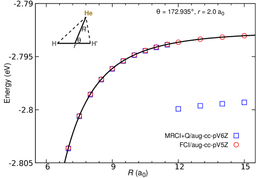
Figure 1: MRCI+Q/aug-cc-pV6Z and FCI/aug-cc-pV5Z energies as a function of $R$ for fixed $\theta=172.935^{\circ}$ and $r=2.0$ a₀. The black line is the RKHS interpolation of the FCI energies

Full CI calculations are smooth out to $R\sim 50$ a₀, contrary to MRCI+Q, see Figure 1. Hence, the full 3-dimensional PES was also calculated using FCI using a somewhat smaller basis set, i.e., aug-cc-pV5Z. This PES, called FCI in the following, was again represented as a RKHS. Although the FCI energies are smooth in the $R-$long range, a third PES (FCI+LR) was constructed by using the same long range expression used for the MRCI+Q+LR PES. For the FCI+LR PES the parameter values in the switching function were $R_{0}=13.5$ a₀ and $\delta R=0.25$ a₀ in Eq. 13.

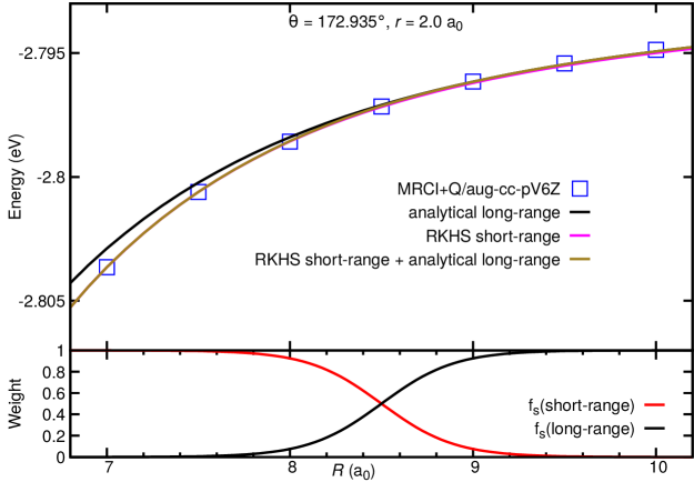
Figure 2: Upper panel: Energies obtained from MRCI+Q/aug-cc-pV6Z, RKHS, analytical long-range and RKHS+analytical are plotted as a function of $R$ for fixed $\theta=172.935^{\circ}$ and $r=2.0$ a₀. Lower panel: the weights for the short range interaction energies and long range interaction energies as a function of $R$.

II.2 Bound state calculations

Ro-vibrational bound state calculations for different $J$ states with $e$ and $f$ symmetries are carried out in scattering coordinates using the 3D discrete variable representation (DVR) method with the DVR3D program suite.Tennyson et al. (2004) The radial Gauss-Laguerre quadrature grids consist of 86 and 32 points along $R$ and $r$ coordinates, respectively. For the Jacobi angle $\theta$, a grid of 36 Gauss-Legendre points was used and for the radial grids ($r$, $R$) the wavefunctions were constructed using Morse oscillator functions. For the diatom (H${}_{2}^{+}$), $r_{e}=2.5$ a₀, $D_{e}=0.1026$ $E_{\rm h}$ and $\omega_{e}=0.018$ $E_{\rm h}$ are used and with these parameters the $r-$grid covered points between 0.92 to 3.8 a₀. As the wave functions for the near-dissociation states need to cover large values along $R$, the corresponding values were $R_{e}=11.5$ a₀, $D_{e}=0.08$ $E_{\rm h}$, and $\omega_{e}=0.00065$ $E_{\rm h}$ which defined the $R$ grid between 1.82 and 20.87 a₀. The $r_{2}$ embeddingTennyson et al. (2004) is used to calculate the rotationally excited states, where the $z-$axis is parallel to $R$ in body-fixed Jacobi coordinates. For the $J>0$ calculations, the Coriolis couplings are included. In the $r_{2}$ embedding, calculations with $ipar=1$ and 0 correspond to the $ortho$ and $para$ H${}_{2}^{+}$, respectively. The $e$ and $f$ symmetries are assigned by the parity operator $p$.

Another method by which we calculated the bound states is the coupled-channels variational method (CCVM). It is similar to a coupled-channels (CC) scattering calculation, but instead of propagating the radial coordinate $R$ to solve the CC differential equations it uses a basis also in $R$ and obtains the desired number of eigenstates of the Hamiltonian matrix with the iterative Davidson algorithm Davidson (1975). For the angular motion of H${}_{2}^{+}$ in the H${}_{2}^{+}$–He complex we used a free rotor basis with $j_{H_{2}^{+}}$ ranging from 0 to 14 (or 16, in tests). The basis in the H${}_{2}^{+}$ vibrational coordinate $r$ contains the $v=0-7$ eigenfunctions of the free H${}_{2}^{+}$ Hamiltonian for $j_{H_{2}^{+}}=0$ on a grid of 110 equidistant points with $r=0.25-5.5~{}a_{0}$. The basis in $R$ was obtained by solving a one-dimensional (1D) eigenvalue problem with the radial kinetic energy and a potential $V_{\rm eff}(R)$. This potential is a cut through the full 3D potential of He-H${}_{2}^{+}$ with $\theta$ and $r$ fixed at the equilibrium values, to which we added a term linear in $R$ with a slope that was variationally optimized by using the $R$ basis in full 3D calculations of the lower He-H${}_{2}^{+}$ levels. The 1D radial eigenvalue problem was solved with sinc-DVR Groenenboom and Colbert (1993) on a 357-point grid with $R=2-50~{}a_{0}$. In order to converge also near-dissociative states we finally included 120 radial basis functions in the 3D full direct product basis.

III Results and Discussion

III.1 Quality of the PESs

First, the quality of the ab initio calculations and their RKHS representation is considered. In Figure 3 the analytical energies are compared with the ab initio energies for a few selected Jacobi angles at $r=2.0$ a₀ for the MRCI+Q+LR PES. A similar comparison is also shown for the FCI PES in Figure S1. Excellent agreement between the two sets of data is found, see Figure 3. Figure S2 presents the contour plot of the analytical energies for the He-H${}_{2}^{+}$ system for $r=2.0$ a₀.

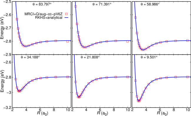
Figure 3: The analytical energies obtained from MRCI+Q+LR PES (solid lines) and the MRCI+Q/aug-cc-pV6Z ab initio energies as a function of $R$ for several Jacobi angles and at fixed $r=2.0$ a₀.

The quality of the RKHS representation of the MRCI+Q+LR and FCI PES is reported in Figure S3. For the grid points used to generate the RKHS representation, the agreement between reference points and the reproducing kernel is excellent with $R^{2}$ values of $(1-2\times 10^{-9})$ and $(1-3\times 10^{-12})$ for MRCI+Q+LR and FCI PESs, respectively. In addition, ab initio energies were also calculated at the MRCI+Q/aug-cc-pV6Z and FCI/aug-cc-pV5Z level of theory for off-grid geometries. They are also reported in Figure S3 together with the RKHS energies evaluated at these geometries. Again, the agreement between the electronic structure calculations and the RKHS representation is good with $R^{2}$ value of $(1-2\times 10^{-7})$ for the MRCI+Q+LR PES.

The equilibrium geometry of the FCI/aug-cc-pV5Z surface is a linear He–H-H configuration ($r=2.0749$ a₀ and $R=2.9712$ a₀), with an energy of –2735.1 cm^-1 below the H${}_{2}^{+}$ asymptote. This compares with the MRCI+Q+LR calculations for which $r=2.0745$ a₀, $R=2.9713$ a₀ and depth –2736.2 cm^-1 and the earlier QCISD(T)/aug-cc-pvQz PESMeuwly and Hutson (1999) ($r=2.0750$ a₀, $R=2.9720$ a₀ and depth –2717.0 cm^-1) values. Hence, the structures of all PESs differ by less than 0.01 a₀ but the energetics varies over a range of $\sim 20$ cm^-1 whereby the dissociation energies for the two PESs from the present work only differ by 1.1 cm^-1.

III.2 Bound States

The ground state energy of H${}_{2}^{+}$($v=0,j=0)$–He computed from the MRCI+Q+LR surface for $ortho-$H${}_{2}^{+}$–He using DVR3D and CCVM are –1795.1567 and –1795.3328 cm^-1, respectively. The same energies, are obtained from the FCI PES as –1793.7632 and –1793.9067 cm^-1, using DVR3D and CCVM, respectively. These values are $\sim 40$ cm^-1 lower compared to those reported previouslyMeuwly and Hutson (1999) (–1754.269 cm^-1) on the QCISD(T) PES. In Ref.Meuwly and Hutson (1999) only 3 quadrature points along $r$ were used for the 3D bound state calculations, which may not be sufficient to fully converge the energies. The ground state energy is also calculated in the present work following a time dependent wave packet approachKoner et al. (2016) on a 2D potential fixing $r$ at 2.0 a₀. These ground state energies are in fair agreement with previous results (–1603 vs. –1593 cm^-1).Meuwly and Hutson (1999)

For para- H${}_{2}^{+}$–He the ground state energies obtained from the MRCI+Q+LR PES using DVR3D and CCVM are –1795.1575 and –1795.3352 cm^-1, respectively. For the FCI surface the ground state energies of para- H${}_{2}^{+}$–He are calculated as –1793.7639 and –1793.9091 cm^-1) using DVR3D and CCVM, respectively. The difference between DVR3D and CCVM is less than 0.17 cm^-1 for both, $ortho$ and $para-$H${}_{2}^{+}$–He. For the FCI+LR PES all the bound states obtained from different methods for both, $ortho$ and $para-$H${}_{2}^{+}$–He are within 0.02 cm^-1 or less of the FCI PES results. Hence, only the results obtained from the MRCI+Q+LR and FCI PESs are reported.

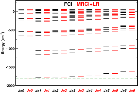
Figure 4: Bound state energies for $J=0\dots 6$ for ortho-H${}_{2}^{+}$-He with $e$ symmetry). Results on the MRCI+Q+LR surface (black) and FCI (red) are shown. The ground state energy (–1793.7632 cm⁻¹) for the FCI/aug-cc-pv5Z surface is marked with a dashed line.

A direct comparison for all and the near-dissociative (within 20 cm^-1 of dissociation) bound $e$ states for ortho-H${}_{2}^{+}$–He and $J=0$ to $J=6$ from DVR3D calculations and using the MRCI+Q+LR (red) and FCI (black) PESs is given in Figures 4 and 5. All states up to the dissociation limit of $v=0,j=1$ state of H${}_{2}^{+}$ are reported. The level pattern for the two PESs is nearly identical. The distribution of the energy difference $\Delta E$ between the MRCI+LR and the FCI PESs for calculations with DVR3D or CCVM is given in Figure S5.

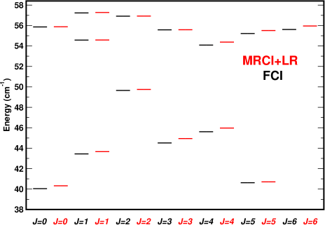
Figure 5: Bound state energies for ($J=0\dots 6$) (ortho) with $e$ symmetry. With MRCI+Q+LR surface (black) and FCI (red). States within $\sim 20$ cm^-1 of the dissociation are reported.

The transitions that were probed by the microwave experiments lie close to dissociation. Hence, a particular focus here is on accurately computing these stationary states and to determine whether any candidate transitions can be identified from using the MRCI+Q+LR and the FCI PESs. A tentative assignment in particular for the 15.2 GHz and 21.8 GHz transitions has been given previously based on experiments using electric field dissociation.Gammie, Page, and Shaw (2002) They were analyzed using an effective Hamiltonian. The 15.2 GHz transition was assigned to a low-$N$ transition (in the terminology of Ref.Gammie, Page, and Shaw (2002), $N$ is the spin-free angular momentum which is $J$ in the present work) with $\Delta N=0$ with $N=3$ or $N=4$ in ortho-H${}_{2}^{+}$–He. In the following, $N$ is used when referring to the analysis of the experimentsGammie, Page, and Shaw (2002) whereas $J$ is used when discussing the present calculations. The fine and hyperfine splittings due to coupling of electron and total nuclear spin, and coupling of the resultant to the rotational angular momentum of the nuclei are both less than 100 MHz, so are several orders of magnitude smaller than the separations between rotational levels of the complex. Thus, identification of $N$ with $J$ is a meaningful approximation.

For the 21.7 GHz transition on the other hand the analysis led to an assignment involving $\Delta N=1$ with $N=11$ and $N^{\prime}=10$ in para-H${}_{2}^{+}$–He. While the analysis leading to a $\Delta N=1$ transition involving para- H${}_{2}^{+}$ is based on physical grounds, that to a high-$N$ state involves fitting of the Zeeman pattern which is more approximate. The selection rules for these transitions are $e\leftrightarrow f$ for $\Delta J=0$ and $e\leftrightarrow e$ or $f\leftrightarrow f$ for $\Delta J=\pm 1$, respectively.

First, the near-dissociative states for ortho-H${}_{2}^{+}$–He are discussed. All near-dissociative states from the MRCI+Q+LR and FCI PESs using the DVR3D and CCVM methods are reported in Figures 6a to d. All energies for $J=0$ to 6 are also reported in Tables 2 and 3. There is one $e/f$ parity doublet with $\Delta J=0$ with a transition frequency between 10 and 18 GHz, involving the $J=2$ state for ortho-H${}_{2}^{+}$–He. Using DVR3D the transition frequency is 14.4(5) GHz whereas with the CCVM code the transition is at 9.3 GHz. The parity doublet in both cases is within 2 cm^-1 of dissociation which makes it a pair of near-dissociative states. This is also confirmed by considering the expectation value for the $R-$coordinate for the two states involved which are $\langle R\rangle=13.1$ a₀ for the $e$ state and $\langle R\rangle=12.7$ a₀ for the $f$ state which confirms their long range character as suggested from the experiments.

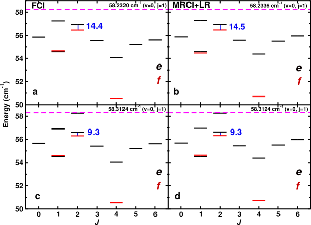
Figure 6: Near dissociation ortho-H${}_{2}^{+}$–He states (in cm^-1) and predicted transition frequencies in (GHz) using the MRCI+Q+LR (left, panels a and c) and FCI/aug-cc-pv5 (right, panels b and d) PESs. States with e (red) and f symmetry (black) are reported separately. Results from DVR3D and CCVM are in the top and bottom row, respectively. The 14.4(5) and 9.3 GHz parity doublet is a candidate for the 15.2 GHz line observed experimentally which had been assigned to a parity doublet with $\Delta N=0$.Gammie, Page, and Shaw (2002)

Next, the near-dissociative states for para-H${}_{2}^{+}$–He are discussed for the two PESs and the two methods to compute bound states, see Figures 7a to d. The only near-dissociative states involving either an $e/e$ or an $f/f$ transition with a transition frequency around 20.1(2) and 16.7(6) GHz from DVR3D and CCVM involves a $J=0$ and a $J=1$ state. The $\langle R\rangle=15.0$ a₀ for the $J=0,e$ state and $\langle R\rangle=16.0$ a₀ for the $J=1,f$ state, show the long range nature of the wave functions. The potential candidate for the 21.8 GHz transition is not found for the high $J$ states sufficiently close to dissociation to be part of a suitable candidate transition.

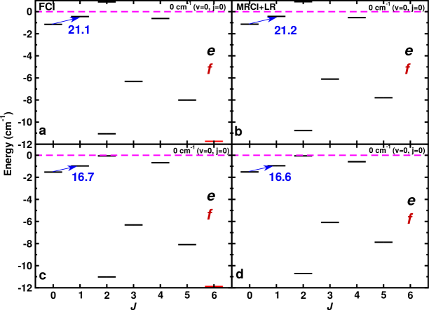
Figure 7: Near dissociation para-H${}_{2}^{+}$–He states (in cm^-1) and predicted transition frequencies in (GHz) using the MRCI+Q+LR (left, panels a and c) and FCI/aug-cc-pv5 (right, panels b and d) PESs. States with e (red) and f symmetry (black) are reported separately. Results from DVR3D and CCVM are in the top and bottom row, respectively.

Table 2: Near dissociation states calculated using MRCI surface with DVR3D and CCVM for He-H${}_{2}^{+}$ in cm^-1. Zero is set to the energy of H${}_{2}^{+}$($v=0,j=0$) state. The dissociation limit for $ortho$ is at 58.2336 cm^-1 and 58.3124 cm^-1 for the DVR3D and CCVM respectively, which corresponds to H${}_{2}^{+}$($v=0,j=1$), whereas the dissociation limit for para- is at 0 cm^-1 which corresponds to H${}_{2}^{+}$($v=0,j=0$).

ortho					para
$e$			$f$		$e$		$f$
$J$	CCVM	DVR3D	CCVM	DVR3D	CCVM	DVR3D	CCVM	DVR3D
0	39.896	40.321			–15.641	–15.719
	55.689	55.876			–1.509	–1.137
1	43.199	43.668	54.629	54.464	–13.965	–14.035
	54.514	54.582			–0.954	–0.430
	56.959	57.273
2	49.345	49.755	56.329	56.439	–10.712	–10.766
	56.639	56.923			–0.061	0.895
	58.272	59.186
3	44.938	44.941	41.798	41.783	–6.082	–6.109
	55.443	55.588
4	46.022	45.971	50.718	50.712	–0.587	–0.540
	54.375	54.375
5	40.655	40.711	40.682	40.680	–7.877	–7.799
	55.518	55.507
6	55.985	55.959					–13.897	–13.746

Table 3: Near dissociation states calculated using FCI surface with DVR3D and CCVM for He-H${}_{2}^{+}$ in cm^-1. Zero is set to the energy of H${}_{2}^{+}$($v=0,j=0$) state. The dissociation limit for $ortho$ is at 58.2320 cm^-1 and 58.3124 cm^-1 for the DVR3D and CCVM respectively, which corresponds to H${}_{2}^{+}$($v=0,j=1$), whereas the dissociation limit for $para$ is at 0 cm^-1 which corresponds to H${}_{2}^{+}$($v=0,j=0$).

$ortho$					$para$
$e$			$f$		$e$		$f$
$J$	CCVM	DVR3D	CCVM	DVR3D	CCVM	DVR3D	CCVM	DVR3D
0	39.575	40.036			–16.005	–16.067
	55.662	55.860			–1.527	–1.150
1	42.934	43.438	54.601	54.648	–14.315	–14.368
	54.494	54.575			–0.969	–0.448
	56.916	57.232
2	49.213	49.647	56.314	56.437	–11.021	–11.058
	56.623	56.916			–0.061	0.881
	58.271	59.162
3	44.497	44.513	41.473	41.473	–6.311	–6.320
	55.422	55.577
4	45.652	45.611	50.538	50.547	–0.680	–0.619
	54.067	54.084
5	40.565	40.626	40.854	40.860	–8.092	–8.005
	55.219	55.220
6	55.626	56.610					–11.890	–11.742

IV Conclusions

Two new PESs at the MRCI+Q+LR and FCI level of theory with large basis sets and represented as a reproducing kernel have been used to determine all bound and near-dissociative states for ortho- and para-H${}_{2}^{+}$–He. It is found that at both levels of theory the bound states compare to within fractions of a wavenumber when stationary states are determined from the same nuclear quantum code. Moreover, the stationary states on one and the same PES determined from two different quantum bound state codes (DVR3D and CCVM) also agree closely, typically within less than fractions of one cm^-1. This provides stringent benchmarks on potential transitions that have been observed experimentally. One such assignment is for the 15.2 GHz transition which corresponds to ortho-H${}_{2}^{+}$–He. The transition found in the present work involves an $e/f$ parity doublet with $J=2$. This compares with a tentative assignment to an $e/f$ parity doublet involving either a $J=3$ or $J=4$ state. For the 21.8 GHz transition which had been tentatively assigned to an $e/e$ or $f/f$ transition in para-H${}_{2}^{+}$–He the candidate, near-dissociation states are $J=0$ and $J=1$, both of which are within less than 2 cm^-1 of dissociation and the transition frequencies range from 16 to 22 GHz. However, no high $J-$ candidate states suitable for transition were found.

The present work presents two high-accuracy, fully dimensional PESs for H${}_{2}^{+}$–He together with quantum bound state calculations that provide potential assignments of experimentally characterized, near-dissociation states. The results from both, MRCI+LR and full CI PESs, using two different approaches for calculating the quantum bound states are largely consistent. It will be interesting to use the present PESs in future inelastic scattering calculations.

Conflicts of interest

There are no conflicts of interest to declare.

References

- Tielens (2013) A. G. G. M. Tielens, Rev. Mod. Phys. 85, 1021 (2013).
- Li, Jiang, and Hao (2015) Q. Li, J. Jiang, and J. Hao, Kona Powder Part. J. 32, 57 (2015).
- Guesten et al. (2019) R. Guesten, H. Wiesemeyer, D. Neufeld, K. M. Menten, U. U. Graf, K. Jacobs, B. Klein, O. Ricken, C. Risacher, and J. Stutzki, Nature 568, 357 (2019).
- Zygelman, Stancil, and Dalgarno (1998) B. Zygelman, P. C. Stancil, and A. Dalgarno, Astrophys. J. 508, 151 (1998).
- Black (2012) J. H. Black, Philos. Trans. Royal Soc. A 370, 5130 (2012).
- Lepp, Stancil, and Dalgarno (2002) S. Lepp, P. C. Stancil, and A. Dalgarno, J. Phys. B: At. Mol. Opt. Phys. 35, R57 (2002).
- Vera et al. (2017) M. H. Vera, F. A. Gianturco, R. Wester, H. da Silva, Jr., O. Dulieu, and S. Schiller, J. Chem. Phys. 146 (2017).
- Koelemeij et al. (2007) J. C. J. Koelemeij, B. Roth, A. Wicht, I. Ernsting, and S. Schiller, Phys. Rev. Lett. 98, 173002 (2007).
- Schiller, Bakalov, and Korobov (2014) S. Schiller, D. Bakalov, and V. I. Korobov, Phys. Rev. Lett. 113, 023004 (2014).
- Klein et al. (2017) A. Klein, Y. Shagam, W. Skomorowski, P. S. Zuchowski, M. Pawlak, L. M. C. Janssen, N. Moiseyev, S. Y. T. van de Meerakker, A. van der Avoird, C. P. Koch, and E. Narevicius, J. Chem. Phys. 13, 35 (2017).
- Carrington et al. (1996) A. Carrington, D. I. Gammie, A. M. Shaw, S. M. Taylor, and J. M. Hutson, Chem. Phys. Lett. 260, 395 (1996).
- Gammie, Page, and Shaw (2002) D. I. Gammie, J. C. Page, and A. M. Shaw, J. Chem. Phys. 116, 6072 (2002).
- Joseph and Sathyamurthy (1987) T. Joseph and N. Sathyamurthy, J. Chem. Phys. 86, 704 (1987).
- Falcetta and Siska (1999) M. F. Falcetta and P. E. Siska, Mol. Phys 97, 117 (1999).
- Meuwly and Hutson (1999) M. Meuwly and J. M. Hutson, J. Chem. Phys. 110, 3418 (1999).
- Palmieri et al. (2000) P. Palmieri, C. Puzzarini, V. Aquilanti, G. Capecchi, S. Cavalli, D. de Fazio, A. Aguilar, X. Giménez, and J. M. Lucas, Mol. Phys. 98, 1835 (2000).
- Ramachandran et al. (2009) C. Ramachandran, D. D. Fazio, S. Cavalli, F. Tarantelli, and V. Aquilanti, Chem. Phys. Lett. 469, 26 (2009).
- de Fazio et al. (2012) D. de Fazio, M. de Castro-Vitores, A. Aguado, V. Aquilanti, and S. Cavalli, J. Chem. Phys. 137, 244306 (2012).
- Werner and Knowles (1988) H. Werner and P. J. Knowles, J. Chem. Phys. 89, 5803 (1988).
- Knowles and Werner (1988) P. J. Knowles and H.-J. Werner, Chem. Phys. Lett. 145, 514 (1988).
- Wilson, van Mourik, and Dunning (1996) A. K. Wilson, T. van Mourik, and T. H. Dunning, J. Mol. Struct. (Theochem) 388, 339 (1996).
- Knowles and Handy (1984) P. Knowles and N. Handy, Chem. Phys. Lett. 111, 315 (1984).
- Knowles and Handy (1989) P. J. Knowles and N. C. Handy, Comput. Phys. Commun. 54, 75 (1989).
- Dunning (1989) T. H. Dunning, J. Chem. Phys. 90, 1007 (1989).
- Woon and Dunning (1994) D. E. Woon and T. H. Dunning, J. Chem. Phys. 100, 2975 (1994).
- Werner and Knowles (1985) H. Werner and P. J. Knowles, J. Chem. Phys. 82, 5053 (1985).
- Knowles and Werner (1985) P. J. Knowles and H.-J. Werner, Chem. Phys. Lett. 115, 259 (1985).
- Werner and Meyer (1980) H. Werner and W. Meyer, J. Chem. Phys. 73, 2342 (1980).
- Werner et al. (2012) H.-J. Werner, P. J. Knowles, G. Knizia, F. R. Manby, and M. Schütz, Wiley Interdiscip. Rev.: Comput. Mol. Sci. 2, 242 (2012).
- Varandas (1988) A. J. C. Varandas, Adv. Chem. Phys. 74, 255 (1988).
- Aguado and Paniagua (1992) A. Aguado and M. Paniagua, J. Chem. Phys. 96, 1265 (1992).
- Bishop and Pipin (1995) D. M. Bishop and J. Pipin, Chem. Phys. Lett. 236, 15 (1995).
- Velilla et al. (2008) L. Velilla, B. Lepetit, A. Aguado, A. Beswick, and M. Paniagua, J. Chem. Phys. 129, 084307 (2008).
- Press et al. (1992) W. H. Press, S. A. Teukolsky, W. T. Vetterling, and B. P. Flannery, Numerical Recipes in Fortran 77 (Cambridge University Press, New York, 1992).
- Ho and Rabitz (1996) T.-S. Ho and H. Rabitz, J. Chem. Phys. 104, 2584 (1996).
- Unke and Meuwly (2017) O. T. Unke and M. Meuwly, J. Chem. Inf. Model 57, 1923 (2017).
- Tennyson et al. (2004) J. Tennyson, M. A. Kostin, P. Barletta, G. J. Harris, O. L. Polyansky, J. Ramanlal, and N. F. Zobov, Comput. Phys. Commun. 163, 85 (2004).
- Davidson (1975) E. R. Davidson, J. Comput. Phys. 17, 87 (1975).
- Groenenboom and Colbert (1993) G. C. Groenenboom and D. T. Colbert, J. Chem. Phys. 99, 9681 (1993).
- Koner et al. (2016) D. Koner, L. Barrios, T. González-Lezana, and A. N. Panda, J. Chem. Phys. 144, 034303 (2016).