Fredholm theory for the mean first-passage time of integrate-and-fire oscillators with colored noise input

Abstract

We develop a method to investigate the effect of noise timescales on the first-passage time of nonlinear oscillators. Using Fredholm theory, we derive an exact integral equation for the mean event rate of a leaky-integrate-and-fire oscillator that receives constant input and temporally correlated noise. Furthermore, we show that Fredholm theory provides a unified framework to determine system scaling behavior for small and large noise timescales. In this framework, the leading order and higher-order asymptotic corrections for slow and fast noise are naturally emerging. We show the scaling behavior in the both limits are not reciprocal. We discuss further how this approach can be extended to study the first-passage time in a general class of nonlinear oscillators driven by colored noise at arbitrary timescales.

The dynamics of nonlinear oscillators that receive temporally correlated inputs plays a central role in the analysis of many physical, chemical and biological systems Wax (1954); *kampen_stochastic_2007; *risken_fokker-planck_1996. The standard method that is used to treat stochastic dynamics that are governed by temporally correlated noise is to approximate the probability law of the system using a Fokker-Planck-like evolution equation (FPE) Moss and McClintock (1989); Häunggi and Jung (1994); Doering et al. (1987); *klosek_colored_1998; *hagan_explicit_1999. Most existing analysis is only applicable when the noisy input correlation time is either much shorter or much longer than the oscillator intrinsic timescale Häunggi and Jung (1994). Many challenging and interdisciplinary questions remain regarding the analysis of stochastic dynamics in the case of nonlinear systems with noise that has intermediate timescales.

In this letter, we determine the mean event rate of a specific nonlinear oscillator: a leaky-integrate-and-fire (LIF) neuron that receives input which fluctuates over arbitrary timescales. Although the LIF is used widely in the mathematical description and numerical simulations of neural circuits Brunel and Rossum (2007); *teeter_generalized_2018, a precise analytical approach that yields the exact system response at all correlation timescales has not yet been developed. We use a mathematical approach that is based on Fredholm theory Fredholm (1903) to address this gap. Our method yields an effective transfer function in the form of an integral equation for arbitrary noise correlation times. Furthermore, our method readily provides an asymptotic expansion term for system limiting behavior in the fast noise case, similar to previous results Brunel and Sergi (1998); *fourcaud_dynamics_2002; *schuecker_modulated_2015. We also, for the first time, derive an asymptotic expansion in the slow noise limit. Our results enable us to understand the interplay between finite noise timescales when shaping nonlinear system dynamics.

We consider the dynamics of an LIF oscillator whose membrane voltage, $x$, and input variable, $y$, satisfyies

$$\frac{d}{dt}x = \alpha_{m}\left[\mu-x+\sqrt{\frac{\alpha_{m}+\alpha_{s}}{\alpha_{m}}}\sigma y\right]$$

$$\frac{d}{dt}y = -\alpha_{s}y+\sqrt{\alpha_{s}}\eta(t),$$ (1)

where $\alpha_{m}=1/\tau_{m}$ and $\alpha_{s}=1/\tau_{s}$. Here, $\tau_{m}$ is the membrane time constant, $\tau_{s}$ is the noise correlation time, $\eta(t)$ is the white noise random variable, and $\sigma$ is the noise amplitude. An oscillator emits an event whenever the membrane reaches the threshold, $x(t^{-})=x_{th}=1$; in this case, the voltage returns immediately to the resting potential (reset), $x(t^{+})=0$. The input scaling factor $\sqrt{\frac{\alpha_{m}+\alpha_{s}}{\alpha_{m}}}$ ensures that the input fluctuation does not die out in the limit $\tau_{s}\rightarrow\infty$, and the equilibrium distribution of $y$ is $P_{y}=e^{-y^{2}}/\sqrt{\pi}$. Additionally, in the absence of an event as $x_{th}\to\infty$, the equilibrium distribution of $x$ is independent of $\alpha_{s}$ and is given by $P_{x}=e^{-(x-\mu)^{2}/\sigma^{2}}/(\sqrt{\pi}\sigma)$.

The standard approach to analyzing Eq. (1) is to study its FPE, as follows:

$$\frac{\partial}{\partial t}\rho(x,y,t)= - \frac{\partial}{\partial x}J_{x}(x,y,t)-\frac{\partial}{\partial y}J_{y}(x,y,t)$$ (2)

$$+ \big{[}\delta(x)-\delta(x-1)\big{]}r(y,t),$$

where $\rho(x,y,t)$ is the probability density of the system being in the state $(x,y)$ at time $t$, $J_{x}(x,y,t)=\aleph_{x}\,\rho(x,y,t)$ and $J_{y}(x,y,t)=\alpha_{s}\left[-y-\frac{1}{2}\frac{\partial}{\partial y}\right]\rho(x,y,t)$ are the flux in $x$ and $y$, respectively, and $\aleph_{x}\equiv\alpha_{m}\left(\mu-x+\sqrt{\frac{\alpha_{m}+\alpha_{s}}{\alpha_{m}}}\sigma\,y\right)$. The reset rate, $r(y,t)$, is the rate at which $x$ reaches the threshold ($x=1$) at noise level $y$ and at time $t$; $r(y,t)$ is given by

$$r(y,t)=J_{x}(1,y,t).$$ (3)

This system of equations has proven difficult to solve directly due to complications associated with the reset mechanism.

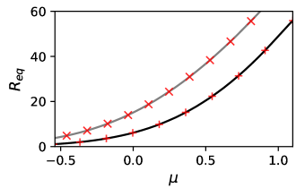
Figure 1: Event rate of an LIF oscillator as a function of mean input for two different synaptic filtering dynamics; the black line indicates $\alpha_{s}=1000$ and the grey line indicates $\alpha_{s}=10$. Symbols are simulation results of an LIF for 1000 trials; error bars are smaller than symbol size. Parameters: $\sigma=1.0$, $\alpha_{m}=100.0$.

To resolve this challenging problem, let $\hat{\rho}(x,y,t|{x^{\prime}},{y^{\prime}},{t^{\prime}})$ be the probability density of state variables $(x,y)$ at time $t$ in the absence of a spiking mechanism, given the initial condition $({x^{\prime}},{y^{\prime}})$ at time ${t^{\prime}}$. Using system invariance under time translation, we observe that this unrestricted probability density is a function of $t-{t^{\prime}}$, and that it can be written as $\hat{\rho}(x,y,t-{t^{\prime}}|{x^{\prime}},{y^{\prime}})$. Moreover, the system without the reset mechanism is simply a linear set of stochastic differential equations with a Gaussian noise variable (Eq. (1)). Thus, $\hat{\rho}$ is completely determined by its mean $(x_{\mathrm{ave}},y_{\mathrm{ave}})$ and its covariance matrix ($C$); details are given in Ref. sup . To include the reset mechanism, we must remove the oscillator at $x=1$ and re-insert it at $x=0$, keeping the value of $y$ unchanged at time ${t^{\prime\prime}}$ with a rate of $r(y,{t^{\prime\prime}}-{t^{\prime}}|{x^{\prime}},{y^{\prime}})$. Therefore, the probability density, $\rho(x,y,t|{x^{\prime}},{y^{\prime}},{t^{\prime}})$ (Eq. (2)) for the oscillator state to be $(x,y)$ at time $t$, given that the state was $({x^{\prime}},{y^{\prime}})$ at time ${t^{\prime}}$, is given by

$$\rho(x,y,t | {x^{\prime}},{y^{\prime}},{t^{\prime}})=\hat{\rho}(x,y,t-{t^{\prime}}|{x^{\prime}},{y^{\prime}})$$ (4)

$$- \int_{t^{\prime}}^{t}\!d{t^{\prime\prime}}\!\int\!d{y^{\prime\prime}}\,[\hat{\rho}(x,y,t-{t^{\prime\prime}}|1,{y^{\prime\prime}})$$

$$- \hat{\rho}(x,y,t-{t^{\prime\prime}}|0,{y^{\prime\prime}})]r({y^{\prime\prime}},{t^{\prime\prime}}-{t^{\prime}}|{x^{\prime}},{y^{\prime}}).$$

Note that Eq.(4) is exact; because Eq.(2) is a linear PDE with the boundary conditions inhomogeneity and Eq.(4) is its solution based on its Green’s function (propagator) Risken and Frank (1996). The rate of oscillator removal at the threshold is, indeed, where $x$ fluxes through $x=1$ from below the threshold. Thus,

$$r(y,t-{t^{\prime}}|{x^{\prime}},{y^{\prime}}) =\left[\aleph_{1}\,\rho(1,y,t-{t^{\prime}}|{x^{\prime}},{y^{\prime}})\right]_{+},$$ (5)

where $[.]_{+}$ is a half-rectification function. Note that, since $\rho$ is non-negative, we obtain $r=0$ for $y<y_{-}\equiv\sqrt{\frac{\alpha_{m}}{\alpha_{m}+\alpha_{s}}}z(1)$, where $z(x)\equiv\frac{(x-\mu)}{\sigma}$. Taking Eq. (5) and inserting $\rho(x,y,t-{t^{\prime}})$ for $x=1$ from Eq. (4) yields a self-consistency equation for $r(y,t-{t^{\prime}}|{x^{\prime}},{y^{\prime}})$. We take the limit ${t^{\prime}}\rightarrow-\infty$ to obtain the equilibrium value for $r$; $r(y,t-{t^{\prime}}|{x^{\prime}},{y^{\prime}})$ and $\hat{\rho}(x,y,t-{t^{\prime}}|{x^{\prime}},{y^{\prime}})$ both reach steady state values in this limit. Note that $r_{\mathrm{eq}}(y)$ and $\hat{\rho}_{\mathrm{eq}}(x,y)$ are independent of ${x^{\prime}}$ and ${y^{\prime}}$, respectively. Furthermore, since $\hat{\rho}(x,y,t|1,{y^{\prime}})-\hat{\rho}(x,y,t|0,{y^{\prime}})$ decays as $e^{-\alpha_{m}t}$ for large $t$, we obtain

$$r_{\mathrm{eq}}(y) = \aleph_{1}\left(\hat{\rho}_{\mathrm{eq}}(1,y)-\int_{y_{-}}^{\infty}\!d{y^{\prime}}\,K(y,{y^{\prime}})r_{\mathrm{eq}}({y^{\prime}})\right),$$ (6)

where the kernel, $K$, is given by

$$K(y,{y^{\prime}})=\int_{0}^{\infty}\!\!dt\,\,\left[\hat{\rho}(1,y,t|1,{y^{\prime}})-\hat{\rho}(1,y,t|0,{y^{\prime}})\right].$$ (7)

Eq. (6) is the Fredholm equation of the second kind. Since we already have expressions for both $\hat{\rho}_{\mathrm{eq}}$ and the kernel $K$ (details are given in Ref. sup ), Eq. ( 6) uniquely determines $r_{\mathrm{eq}}(y)$ for $y\geq y_{-}$. Finally, the output event rate, $R_{\mathrm{eq}}$, which describes that rate at which an oscillator emits spikes at equilibrium, is given by

$$R_{\mathrm{eq}}=\int_{y_{-}}^{\infty}\!dy\,r_{\mathrm{eq}}(y).$$ (8)

The solution to this equation is easily obtained numerically using standard techniques (details are given in Ref. sup ). Figs.1 and 2 illustrate the dependence of the mean event rate on various parameters. In Fig. 1, the output rate, $R_{\mathrm{eq}}$, is plotted against mean input, $\mu$, for two intermediate values of $\tau_{s}$; the rate is reduced for larger $\tau_{s}$. Fig. 2 demonstrates the dependence of $R_{\mathrm{eq}}$ on arbitrary $\tau_{s}$. We observe that the event rate is strongly dependent on synaptic filtering. Fredholm theory for the escape rate (Eq. (6)), presented here, also allows analytical study of the asymptotic behavior, in both the fast and slow noise regimes.

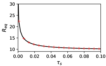
Figure 2: Event rate of an LIF oscillator as a function of synaptic timescale. The black line indicates the output rate obtained by solving Fredholm equation in Eq.(6). The crosses indicate the event rate resulting from numerical simulations of an LIF oscillator over 1000 trials, as described in Eq. 1. Parameters: $\mu=0.2$, $\sigma=1.0$, $\alpha_{m}=100.0$.

To determine the asymptotic correction for the fast noise regime, we must expand $\hat{\rho}_{\mathrm{eq}}(1,y)=\sum_{n=1}^{\infty}\left(\frac{\alpha_{m}}{\alpha_{s}}\right)^{n/2}\hat{\rho}_{f_{n}}^{\mathrm{eq}}(1,y)$ and $K(y,{y^{\prime}})=\sum_{n=1}^{\infty}\left(\frac{\alpha_{m}}{\alpha_{s}}\right)^{n/2}K_{f_{n}}(y,{y^{\prime}})$. We make the Ansatz that $r_{\mathrm{eq}}(y)=\sum_{n=0}^{\infty}(\frac{\alpha_{m}}{\alpha_{s}})^{n/2}r_{f_{n}}(y)$. We obtain

$$\sum_{n=0}^{\infty}\left(\frac{\alpha_{m}}{\alpha_{s}}\right)^{n/2}r_{f_{n}}(y)=\alpha_{m}\sum_{n=-1}^{\infty}\left(\frac{\alpha_{m}}{\alpha_{s}}\right)^{n/2}F_{n}(y)$$ (9)

where, $F_{n}(y)$ collects terms of order $(\frac{\alpha_{m}}{\alpha_{s}})^{n/2}$. Since the right-hand side of Eq. (9) only has terms with $n\geq 0$, we must to impose that $F_{-1}(y)=0$ for $y\geq y_{-}$. Therefore, as shown in Ref. sup , to leading order, the event rate, $R_{f_{0}}\equiv\int_{y_{-}}^{\infty}dy\,r_{f_{0}}(y)$, is given by $R_{f_{0}}=\frac{\alpha_{m}}{I_{R}(z(0),z(1))},$ where $I_{R}(z_{0},z_{1})=2\int_{z_{1}}^{z_{0}}dze^{z^{2}}\int_{z}^{\infty}dz^{\prime}e^{-(z^{\prime})^{2}}$. This is, indeed, the firing rate of an LIF neuron receiving white noise input Ricciardi (1977). To obtain the first order asymptotic correction to the white noise case, we must evaluate $F_{0}(y)$ in Eq. (9); this gives the Fredholm theory for the first order correction. Using the linearity of the Fredholm operator and its resolvent properties in Eq. (9) for $n=1$ (details are given in Ref. sup ), we can write the asymptotic correction of the fast noise limit as

$$R_{f_{1}}=-\frac{\alpha_{m}}{\Phi_{0}I(z(0),z(1))^{2}}J_{R}(z(0),z(1)),$$ (10)

where $J_{R}(z_{0},z_{1})=2\sqrt{\pi}(\exp({z_{0}}^{2})\,\mathrm{erfc}(z_{0})-\exp({z_{1}}^{2})\,\mathrm{erfc}(z_{1}))$ and $\Phi_{0}=\frac{-\sqrt{2}}{\zeta(\frac{1}{2})}$ (up to $10^{-10}$ numerical accuracy, see Ref. sup for details), where $\zeta$ is the Riemann zeta function. This is consistent with previous results Brunel and Sergi (1998); Fourcaud and Brunel (2002); Schuecker et al. (2015), that use boundary layer and half-range expansion theories Doering et al. (1987); Kłosek and Hagan (1998); Hagan and Kłosek (1999). Interestingly, the constant $\Phi_{0}$ corresponds to Milne extrapolation lengths for the FPE Doering et al. (1997). The Eq.(10) yields the linear rate correction $R_{\mathrm{eq}}=R_{f_{0}}+\sqrt{\frac{\alpha_{s}}{\alpha_{m}}}R_{f_{1}}$ in the fast noise limit. Fig. 3 demonstrates the limiting behavior of the event rate in the near white noise regime; the full solution of the Fredholm equation using Eq.(6) (tick red line) and linear asymptotic correction according to Eq.(10) (thin grey line) are plotted against $\sqrt{\frac{\alpha_{m}}{\alpha_{s}}}$. The simulation results shown in Fig. 3 (cross symbols) provide an excellent agreement with the full solution (thick black line).

Figure 3: Fast noise regime for the event rate of an LIF oscillator as a function of $\sqrt{\frac{\alpha_{m}}{\alpha_{s}}}$. The black thick line displays the full solution of Eq.(6) and the thin grey line displays the linear approximation of firing for large and finite $\alpha_{s}$. Crosses are simulations of an LIF for $10^{5}$ trials with a duration of $1000\times\tau_{m}$. Parameters: $\mu=.20$, $\sigma=1.$, $\alpha_{m}=100.0$.

The asymptotic correction in the slow noise regime is also a straightforward application of a perturbation calculation in our approach. In the slow noise limit ($\alpha_{s}\rightarrow 0$), we can assume that the level of noise is constant between two neighboring events and the inter-event-interval is $t_{0}(y)\equiv\alpha_{m}^{-1}[\log(\mu+\sigma y)-\log(\mu+\sigma y-1)]$ for $y>y_{-}$ Moreno et al. (2002); *moreno-bote_role_2004; *moreno-bote_response_2010. Therefore, to leading order, $r_{s_{0}}(y)$ is given by

$$r_{s_{0}}(y) = \frac{P_{\mathrm{eq}}({y})}{t_{0}(y)}=\frac{\alpha_{m}}{\sqrt{\pi}}e^{-y^{2}}\left[\log\left(\frac{\mu+\sigma y}{\mu+\sigma y-1}\right)\right]^{-1}$$ (11)

for $y>y_{-}$, and $r_{s_{0}}(y)=0$ otherwise. Although this result is an already established Moreno et al. (2002); *moreno-bote_role_2004; *moreno-bote_response_2010, to the best of our knowledge, asymptotic correction terms for non-zero but small $\alpha_{s}$ have not yet been determined. To simplify the calculation, we rescale the noise to be independent of $\alpha_{s}$ by setting $\Sigma\equiv\sqrt{\frac{\alpha_{m}+\alpha_{s}}{\alpha_{m}}}\sigma$; dependence on $\alpha_{s}$ can be re-introduced at a later stage. To determine the first order correction in the slow noise case, we observe that, for $\frac{y-y_{-}}{\sqrt{\frac{\alpha_{s}}{\alpha_{m}}}}\gg 1$, $\hat{\rho}_{\mathrm{eq}}(1,y)$ is exponentially small and can be neglected and the kernel $K(y,{y^{\prime}})$ is exponentially small unless ${y^{\prime}}-y$ is of order $\sqrt{\alpha_{s}/\alpha_{m}}$. Therefore, for $\frac{y-y_{-}}{\sqrt{\alpha_{s}/\alpha_{m}}}\gg 1$ we have ${y^{\prime}}\sim y+\sqrt{\frac{\alpha_{s}}{\alpha_{m}}}Y$ in Eq. 6 and using the Taylor expansion in $Y$ of $r_{\mathrm{eq}}(y+\sqrt{\alpha_{s}/\alpha_{m}}Y)$ we can rewrite $r_{\mathrm{eq}}$ as

$$r_{\mathrm{eq}}(y)=\beth\left(\sum_{n=0}^{\infty}\left[\frac{\alpha_{s}}{\alpha_{m}}\right]^{n/2}K_{n}(y)\frac{d^{n}}{dy^{n}}\right)r_{\mathrm{eq}}(y),$$ (12)

where $\beth=-\alpha_{m}[\mu-1+\Sigma y]$, as given in Ref. sup , and $K_{n}$ must be expanded as $K_{n}(y)=\sum_{k=0}^{\infty}\left[\frac{\alpha_{s}}{\alpha_{m}}\right]^{k/2}K_{n,k}(y)$, where $K_{n,k}$ are independent of $\alpha_{s}/\alpha_{m}$. Importantly, $K_{n,k}(y)=0$ when $n+k$ is odd and $\beth K_{0,0}(y)=-1$ (details are given in Ref. sup ). Inserting this in Eq.(12), we obtain

$$\sum_{m=1}^{\infty}\left[\frac{\alpha_{s}}{\alpha_{m}}\right]^{m-1}\sum_{n=0}^{2m}K_{n,2m-n}\frac{d^{n}}{dy^{n}}r_{\mathrm{eq}}(y)=0.$$ (13)

Interestingly, because $K_{n,m}=0$ when $n+m$ is odd, the leading order correction is of order $\alpha_{s}/\alpha_{m}$ rather than $\sqrt{\alpha_{s}/\alpha_{m}}$. Thus, we expand $r_{\mathrm{eq}}$ in powers of $\alpha_{s}/\alpha_{m}$ as

$$r_{eq}(y)=\sum_{n=0}^{\infty}\left[\frac{\alpha_{s}}{\alpha_{m}}\right]^{n}r_{s_{n}}(y).$$ (14)

Inserting Eq. (14) into Eq. (12) and collecting terms with the same power of $\alpha_{s}/\alpha_{m}$, we find that $r_{s_{n}}$ satisfies

$$\mathcal{K}r_{s_{n}}(y)=-S_{n}(y),$$ (15)

where the operator is given by $\mathcal{K}\equiv K_{0,2}(y)+K_{1,1}(y)\frac{d}{dy}+K_{2,0}\frac{d^{2}}{dy^{2}}$ , and for $n\geq 1$, $S_{n}$ satisfies

$$S_{n}(y)=\sum_{k=0}^{n-1}\left[\sum_{\ell=0}^{2(n+1-k)}K_{i,2(n+1-k)-\ell}(y)\frac{d^{\ell}}{dy^{\ell}}\right]r_{s_{k}}(y),$$ (16)

and $S_{0}(y)=0$. Since $\mathcal{K}$ is a second order differential operator, Eq. (15) determines $r_{s_{n}}$ up to two integration constants, provided that all $r_{s_{k}}$ for $k\in\{0,1,\ldots,n-1\}$ are given. This does not completely determine $r_{s_{n}}$ because we have only considered $r_{\mathrm{eq}}$ for $\frac{y-y_{-}}{\sqrt{\alpha_{s}/\alpha_{m}}}\gg 1$. However, we can still determine the asymptotic corrections since we can write the scaling factor $c_{n}\equiv{r_{s_{n}}}/r_{s_{0}}$ and insert it into Eq. 15 and thus $c_{n}$ satisfies

$$\left[\frac{d}{dy}-2y\right]\frac{d}{dy}c_{n}(y)=-s_{n}(y),$$ (17)

where $s_{n}(y)=t_{0}(y)S_{n}(y)/(K_{2,0}(y)P_{\mathrm{eq}}(y))$. This is clearly consistent with $c_{0}(y)=1$ in $r_{s_{0}}(y)=c_{0}(y)P_{\mathrm{eq}}(y)/t_{0}(y)$. For large $y$ and $\frac{y-y_{-}}{\sqrt{\alpha_{s}}t_{0}(y)}\gg 1$, the kernel $K(y,y^{\prime})$ becomes exponentially small; therefore, as $y\rightarrow\infty$, fluctuations in $y$ are negligible for any order $n$. Hence, for $n>0$, $c_{n}(y)\rightarrow 0$ and $\frac{d}{dy}c_{n}(y)\rightarrow 0$ as $y\rightarrow\infty$. Thus, $c_{n}(y)$ satisfies

$$c_{n}(y)=\int_{y}^{\infty}\!dy_{1}e^{y_{1}^{2}}\int_{y_{1}}^{\infty}\!dy_{2}\,s_{n}(y_{2})e^{-y_{2}^{2}}.$$ (18)

This determines the leading order correction, $r_{s_{1}}(y)=c_{1}(y)r_{s_{0}}(y)$ and $s_{1}$ is given in Ref. sup . Here, we obtain Eq.(18) assuming that $\Sigma$ is constant, so the scaling factor can be reformulated as $\tilde{c}_{1}=c_{1}-\frac{y}{2}(\frac{d}{dy}t_{0}(y))/t_{0}(y)$ to return to the original formulation of the problem. Now, using $R_{s_{1}}\equiv\int_{y_{-}}^{+\infty}dy^{\prime}r_{s_{1}}(y^{\prime})$ we obtain $R_{\mathrm{eq}}=R_{s_{0}}+\frac{\alpha_{s}}{\alpha_{m}}R_{s_{1}}$. Fig. 4 illustrates the linear approximation (thin grey line) of the event rate for small but finite $\alpha_{s}$ tangents to the full solution of Fredholm equation (thick black line) in Eq.(6).

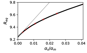
Figure 4: Slow noise regime for the event rate of an LIF oscillator as a function of $\frac{\alpha_{s}}{\alpha_{m}}$. The thick black line is the full solution of Eq.(6) and the thin grey line is its the linear approximation for small and finite $\alpha_{s}$. Mean event rates of numerical simulations of an LIF oscillator for $10^{5}$ trials with a duration of $1000/\alpha_{s}$ are indicated by crosses. Parameters: $\mu=0.2$, $\sigma=1.0$, $\alpha_{m}=100.0$.

In this letter, we studied the nonlinear dynamics of an LIF oscillator that is driven by colored noise. We derived, for the first time, an exact expression for the event rate of the model for arbitrary correlation times in the form of a Fredholm equation, which can readily be evaluated numerically. This approach does not require the separation of timescales and weak noise expansion that are typically assumed in the classical analysis of colored noise in stochastic dynamics Häunggi and Jung (1994); Moss and McClintock (1989). Additionally, we show that Fredholm theory provides a uniform formalism by which to systematically calculate the fast and slow noise asymptotic expansions. These expansions lead to the interesting conclusion that the system exhibits different scaling behaviors in slow and fast noise regimes. Most previous works in the fast noise regime use boundary-layer theory to derive the leading order correction to the mean rate Doering et al. (1987); Kłosek and Hagan (1998); Hagan and Kłosek (1999); Brunel and Sergi (1998); Fourcaud and Brunel (2002); Schuecker et al. (2015). Our approach recovers this result. Formally, application of FPE boundary layer theory requires the assumption that the potential well is smooth and has zero slope at the absorbing upper boundary. Remarkably, our result indicates that the details of the potential do not contribute to the correction term. In the slow noise extreme ($\alpha_{s}\rightarrow 0$), Moreno-Bote et al. Moreno et al. (2002); *moreno-bote_role_2004; *moreno-bote_response_2010 used an adiabatic approach to derive the mean event rate; we have derived the same result. It is noteworthy, Moreno-Bote et al. Moreno-Bote et al. (2008) showed that in the limit of large $\tau_{s}$ and an additional white noise the leading order correction is linear. The unified framework here allows to generalize their results systematically and also calculate the magnitude of the slow noise correction. Our analysis shows that the order of the asymptotic corrections at the both slow and fast noise timescales do not scale reciprocally; the order of limiting behavior for the case of fast noise is $\sqrt{\tau_{s}/\tau_{m}}$, while for slow noise it is $\tau_{m}/\tau_{s}$. Our asymptotic analysis for large and small $\alpha_{s}$ indicates that linear regimes are fall outside the physiological relevant range of synaptic dynamics (Figs.  3 and  4). This demonstrates the importance of the full solution of the Fredholm equation for the investigation of neural network dynamics.

Our approach can be extended to calculate the response of LIF units to infinitesimal non-stationarities in the input. This can be used to evaluate the stability of an asynchronous state of recurrent networks. To this end, one needs to follow the perturbation theory developed in Farkhooi and van Vreeswijk (2015). Furthermore, using Markovian embedding method one can consider a non-exponentially correlated temporal input (for small noise, $\sigma/\mu\ll 1$) Häunggi and Jung (1994) similar to work by Schwalger et al.Schwalger et al. (2015) for the perfect-integrate-and-fire neurons.

Our method can be applied when the solution to the unrestricted process, $\hat{\rho}$, is known. For example, our method can be used in the normative models of decision-making in a dynamic environment that an agent values recent observations more than older one Ossmy et al. (2013); in the case of exponential discounting of the observations, one can directly apply our results. The other interesting example is Kubo’s stochastic model that describes a irreversible process in which the noise variable takes discrete values with a Poisson switching. In Kubo’s model $\hat{\rho}$ is readily determined for an arbitrary drift term Kubo (2007); Häunggi and Jung (1994). This model has been used extensively in analyzing the kinetic theory of gases and the statistical theory of line-broadening Saven and Skinner (1993); *bezzerides_theory_1969. In cases where oscillator dynamics can be described by a motion equation of phase variable, a Fourier expansion of $\hat{\rho}$ is typically available Hongler and Zheng (1982). In this case, an arbitrary-precise solution can be constructed by considering the first $n$ Fourier moments as it has been used to construct a non-Gaussian density in laser gyroscope applications Vogel et al. (1987). More generally, where an exact expression for $\hat{\rho}$ is unavailable, an approximate solution can often be estimated; for example, in exponential and quadratic integrate-and-fire systems Richardson (2007). This approximate solution can be used to obtain an approximate mean first-passage time. Therefore, the approach to cast statistics of nonlinear stochastic oscillators in a form of a Fredholm equation allows analysis of the effects of correlated environmental noise in a diverse range of problems.