Bogoliubov Fermi surfaces stabilized by spin-orbit coupling

Abstract

It was recently understood that centrosymmetric multiband superconductors that break time-reversal symmetry generically show Fermi surfaces of Bogoliubov quasiparticles. We investigate the thermodynamic stability of these Bogoliubov Fermi surfaces in a paradigmatic model. To that end, we construct the mean-field phase diagram as a function of spin-orbit coupling and temperature. It confirms the prediction that a pairing state with Bogoliubov Fermi surfaces can be stabilized at moderate spin-orbit coupling strengths. The multiband nature of the model also gives rise to a first-order phase transition, which can be explained by the competition of intra- and interband pairing and is strongly affected by cubic anisotropy. For the state with Bogoliubov Fermi surfaces, we also discuss experimental signatures in terms of the residual density of states and the induced magnetic order. Our results show that Bogoliubov Fermi surfaces of experimentally relevant size can be thermodynamically stable.

I Introduction

A hallmark of unconventional superconductivity is a nodal pairing state where the excitation gap vanishes at points or lines in momentum space Mineev and Samokhin (1999). Recently, however, a third type of node has been proposed: extended Bogoliubov Fermi surfaces (BFSs) where the excitation gap vanishes at a surface in momentum space Agterberg et al. (2017a); Brydon et al. (2018). In clean, inversion-symmetric (even-parity) superconductors that spontaneously break time-reversal symmetry (TRS), all nodes are generically expected to be BFSs. Crucial for the appearance of BFSs is that the superconductivity involves more than one band: Specifically, the pairing between electrons in different bands generates a pseudomagnetic field, which “inflates” point and line nodes of the intraband pairing potential into BFSs. These nodal surfaces are robust against perturbations that preserve particle-hole and inversion symmetries, which can be formulated in terms of a $\mathbb{Z}_{2}$ topological invariant Kobayashi et al. (2014); Zhao et al. (2016); Agterberg et al. (2017a); Bzdušek and Sigrist (2017).

A natural setting for the appearance of BFSs is in systems where a multiband structure arises from the presence of discrete low-energy electronic degrees of freedom apart from spin, e.g., atomic-orbital or sublattice indices. This permits the construction of novel “internally anisotropic” pairing states where the Cooper-pair wave function has nontrivial dependence upon the orbital or sublattice indices Nomoto et al. (2016); Cheung and Agterberg (2019); Brydon et al. (2018). Crucially, for the appearance of BFSs, internally anisotropic pairing states are typically characterized by both intraband and interband pairing potentials Brydon et al. (2018). Such pairing states have been proposed for a wide variety of multiband systems of current interest, such as iron-based superconductors Gao et al. (2010); Nicholson et al. (2012); Ong et al. (2016); Vafek and Chubukov (2017); Agterberg et al. (2017b); Setty et al. (2019); Hu et al. (2019), Cu_xBi₂Se₃ Fu (2014), half-Heusler compounds Brydon et al. (2016); Agterberg et al. (2017a); Savary et al. (2017); Yang et al. (2017); Roy et al. (2019); Timm et al. (2017); Boettcher and Herbut (2018a, b); Kim et al. (2018); Brydon et al. (2018), the antiperovskite Sr_3-xSnO Kawakami et al. (2018), Sr₂RuO₄ Taylor and Kallin (2012), UPt₃ Nomoto and Ikeda (2016); Yanase (2016), transition-metal dichalcogenides Oiwa et al. (2018); Möckli and Khodas (2018), and twisted bilayer graphene Guo et al. (2018); Su and Lin (2018); Wu (2019). This long list of materials—some of which are believed to support a time-reversal-symmetry-breaking (TRSB) state—is encouraging for the existence of BFSs.

Although BFSs are robust against symmetry-preserving perturbations, this topological protection does not guarantee the existence of such a state. Instead, it is necessary to consider the thermodynamic stability. Since a TRSB combination of two nodal pairing states eliminates all nodes that are not common to both states, it is expected to be energetically favored over time-reversal-symmetric combinations Sigrist and Ueda (1991). This argument does not hold if the resulting TRSB state possesses a BFS, however, as this implies a nonzero density of states (DOS) at the Fermi energy, which, at first glance, is unfavorable compared to the line nodes generic for time-reversal-symmetric states. It was argued in Ref. Agterberg et al. (2017a) that a TRSB state with a BFS could, nevertheless, be energetically favorable in the presence of sufficiently strong spin-orbit coupling (SOC). This analysis was restricted to temperatures close to $T_{c}$, however, and so did not account for the effect of the expected large residual DOS at low temperatures. Moreover, although the TRSB state becomes more stable with increasing SOC, the size of the BFS decreases, as shown below. It is, thus, unclear if BFSs can be realized in a limit where they have a detectable effect on the electronic structure Lapp et al. (2019). Another interesting question raised by the analysis in Refs. Agterberg et al. (2017a); Brydon et al. (2018) is what happens at SOC strengths insufficient for a stable TRSB state.

In this paper, we use mean-field theory to study the appearance of BFSs in a paradigmatic model of a multiband system with strong SOC, specifically the Luttinger-Kohn Hamiltonian of $j=3/2$ fermions in a cubic material Luttinger and Kohn (1955). The $j=3/2$ degree of freedom naturally leads to a multiband system and to internally anisotropic pairing. Assuming pairing in a s-wave $J=2$ channel Brydon et al. (2016), we construct the superconducting phase diagram as a function of the SOC strength and temperature. We focus on a particular set of pairing states belonging to the irreducible representation (irrep) $T_{2g}$, which is expected to provide a typical picture for pairing in a higher-dimensional representation. At vanishing SOC, a fully gapped time-reversal-symmetric superconducting phase is realized as was predicted in Ref. Ho and Yip (1999). For nonzero SOC, we obtain a rich phase diagram, which, in particular, contains a sizable region with TRSB superconductivity. The largest BFSs that we find lead to a residual zero-temperature DOS at the Fermi energy of approximately 20% of the normal-state DOS, which should leave clear signatures in thermodynamic measurements. We also verify the existence of a subdominant magnetic order parameter which is induced by the TRSB superconductivity.

Our paper is organized as follows: In Sec. II, we introduce our microscopic model and outline the mean-field theory, including a discussion of previously known limits of vanishing and strong SOC. We present the mean-field phase diagram in Sec. III and study the effect of cubic anisotropy of the SOC. A key feature of the phase diagram is the first-order transition into a time-reversal-symmetric superconducting state at intermediate SOC strength, which we explain in terms of a simplified model. This is followed in Sec. IV by a detailed study of the TRSB state and the induced magnetic order parameter. We summarize our results and draw additional conclusions in Sec. V.

II Model and mean-field theory

Our starting point is the Luttinger-Kohn Hamiltonian for $j=3/2$ fermions in a cubic material Luttinger and Kohn (1955),

$$h(\bm{k})=(\alpha\lvert\bm{k}\rvert^{2}-\mu)\,\openone_{4}+\beta\sum_{i}k_{i}^{2}J_{i}^{2}+\gamma\sum_{i\neq j}k_{i}k_{j}J_{i}J_{j},$$ (1)

where $i=x,y,z$ and $i+1=y$ if $i=x$, etc., and $J_{i}$ are the $4\times 4$ matrix representations of the angular momentum operators $j=3/2$. The $j=3/2$ fermions can arise due to the strong atomic SOC, e.g., of spins $s=1/2$ and orbital angular momenta $l=1$ for p orbitals. In addition to the spin-independent dispersion coefficient $\alpha$ and the chemical potential $\mu$, the Hamiltonian in Eq. (1) includes the symmetry-allowed SOC terms proportional to $\beta$ and $\gamma$. The Hamiltonian has doubly degenerate eigenvalues given by

$$\epsilon_{\bm{k},\pm} =\biggl{(}\alpha+\frac{5}{4}\,\beta\biggr{)}\lvert\bm{k}\rvert^{2}-\mu$$

$$\quad{}\pm\beta\sqrt{\sum_{i}\biggl{[}k_{i}^{4}+\biggl{(}\frac{3\gamma^{2}}{\beta^{2}}-1\biggr{)}k_{i}^{2}k_{i+1}^{2}\biggr{]}}.$$ (2)

Note that SOC lifts the fourfold degeneracy of the $j=3/2$ manifold away from the $\Gamma$ point. Due to the presence of time-reversal and inversion symmetries, the bands remain doubly degenerate so that the states in each band can be labeled by a pseudospin-$1/2$ index Brydon et al. (2018).

The description in terms of an effective spin $j=3/2$ permits Cooper pairs with total angular momentum $J=0$ (singlet) and $J=1$ (triplet), but also $J=2$ (quintet) and $J=3$ (septet) Boettcher and Herbut (2016); Brydon et al. (2016); Savary et al. (2017); Roy et al. (2019); Yang et al. (2017); Venderbos et al. (2018); Boettcher and Herbut (2018a, b); Kim et al. (2018); Sim et al. (2019). Similar to singlets and triplets, the quintet and septet pairings correspond to even- and odd-parity orbital wave functions, respectively. In particular, this allows for a broader variety of s-wave pairing states: Besides the usual singlet, there are five additional quintet states with on-site pairing.

Restricting ourselves to such local pairing states, the pairing interaction has the general form

$$H_{\text{pair}}=\sum_{j}\sum_{l}\sum_{l_{i}\in l}V_{l}\,b^{\dagger}_{l_{i},j}b_{l_{i},j},$$ (3)

where $b^{\dagger}_{l_{i},j}$ creates a Cooper pair at site $j$ in channel $l_{i}$ belonging to the irrep $l$ Brydon et al. (2016). There are three irreps in the cubic $O_{h}$ point group which support s-wave pairing: The singlet state belongs to the one-dimensional $A_{1g}$ irrep, whereas the five quintet states are distributed into the two-dimensional $E_{g}$ and the three-dimensional $T_{2g}$ irreps.

Within the standard mean-field treatment, the interaction is decoupled to obtain the effective single-particle Hamiltonian,

$$H_{\mathrm{MF}}=\sum_{\bm{k}}\biggl{(}\frac{1}{2}\,\Psi_{\bm{k}}^{\dagger}\mathcal{H}(\bm{k})\Psi_{\bm{k}}+\sum_{l}\frac{\operatorname{Tr}[\Delta_{l}\Delta_{l}^{\dagger}]}{V_{l}}\biggr{)},$$ (4)

with the Bogoliubov–de Gennes (BdG) Hamiltonian,

$$\mathcal{H}(\bm{k})=\begin{pmatrix}h(\bm{k})&\Delta\\ \Delta^{\dagger}&-h^{T}(-\bm{k})\\ \end{pmatrix},$$ (5)

and the Nambu spinors $\Psi_{\bm{k}}=(c_{\bm{k}},c_{-\bm{k}}^{\dagger})^{T}$ with $c_{\bm{k}}=(c_{\bm{k},3/2},\allowbreak c_{\bm{k},1/2},\allowbreak c_{\bm{k},-1/2},\allowbreak c_{\bm{k},-3/2})^{T}$, where $c_{\bm{k},\sigma}$ is the annihilation operator for a fermion with momentum $\bm{k}$ and spin $\sigma$.

In this paper, we focus on pairing states in the $T_{2g}$ irrep, where a general pairing state can be written as

$$\Delta=\Delta_{0}\,(l_{yz}\eta_{yz}+l_{xz}\eta_{xz}+l_{xy}\eta_{xy}),$$ (6)

with the amplitude $\Delta_{0}$, the three-component order parameter $\bm{l}=(l_{yz},\allowbreak l_{xz},\allowbreak l_{xy})$, and the gap matrices $\eta_{\alpha\beta}=(J_{\alpha}J_{\beta}+J_{\beta}J_{\alpha})U_{T}/\sqrt{3}$, where

$$U_{T}=\begin{pmatrix}0&0&0&1\\ 0&0&-1&0\\ 0&1&0&0\\ -1&0&0&0\\ \end{pmatrix}$$ (7)

is the unitary part of the time-reversal operator. From the fourth-order expansion of the corresponding Landau free energy, four possible ground states are known: $\bm{l}=(1,0,0)$, $(1,1,1)$, $(1,i,0)$, and $(1,\omega,\omega^{2})$ with $\omega=e^{2\pi i/3}$ (as well as symmetry-related vectors) Sigrist and Ueda (1991). The states $(1,0,0)$ and $(1,1,1)$ are time-reversal symmetric, whereas the chiral state $(1,i,0)$ and the cyclic state $(1,\omega,\omega^{2})$ break TRS and, therefore, support BFSs Brydon et al. (2018). In the following, however, we focus on the submanifold of $T_{2g}$ states spanned by the $\bm{l}=(1,0,0)$ and $(1,i,0)$ states by adopting the mean-field ansatz:

$$\Delta=\Delta_{yz}\eta_{yz}+i\Delta_{xz}\eta_{xz},$$ (8)

with two real variational parameters $\Delta_{xz}$ and $\Delta_{xz}$. If one of the parameters is zero, we obtain the TRS-preserving $\bm{l}=(1,0,0)$ state. On the other hand, a TRSB state is realized if both parameters are nonzero; in particular, the case of $\Delta_{yz}=\Delta_{xz}$ corresponds to $\bm{l}=(1,i,0)$. Although this restricted ansatz is artificial for a cubic system, we are motivated by the observation that the $\eta_{xz}$ and $\eta_{yz}$ pairing potentials are the only s-wave quintet states in our cubic model which are also degenerate in hexagonal and tetragonal crystals. For example, a chiral d-wave state with the same symmetry is believed to be realized in tetragonal URu₂Si₂ Kasahara et al. (2007). We, therefore, expect our conclusions to be applicable to any TRSB superconductor with two degenerate pairing potentials. The $(1,i,0)$ state has an (inflated) equatorial line node, which should lead to a higher free energy compared to a state with only (inflated) point nodes. By considering the likely less favorable pairing state, we, at worst, underestimate the stability of the BFSs. In fact, performing the same analysis for the pair of $E_{g}$ states does not result in qualitative changes in the phase diagram. The pairing state in the spherically symmetric limit has been considered in Refs. Boettcher and Herbut (2016, 2018a); Herbut et al. (2019).

II.1 Free energy

In a weak-coupling approach, the leading pairing instability can be obtained by direct minimization of the Helmholtz free energy with respect to the mean fields. From the BdG Hamiltonian (4), we obtain the Helmholtz free energy

$$F=\sum_{\bm{k}}\frac{\operatorname{Tr}[\Delta\Delta^{\dagger}]}{V_{0}}-2k_{B}T\sum_{\bm{k},\nu}\ln\biggl{[}2\cosh\biggl{(}\frac{E_{\bm{k},\nu}}{2k_{B}T}\biggr{)}\biggr{]},$$ (9)

where $V_{0}$ is the attractive pairing interaction in the $T_{2g}$ channel and $E_{\bm{k},\nu}$ are the positive eigenvalues of $\mathcal{H}(\bm{k})$ in Eq. (5). Inserting the mean-field ansatz from Eq. (8), we numerically minimize the Helmholtz free energy to obtain the self-consistent values of $\Delta_{xz}$ and $\Delta_{yz}$.

To compare with our numerical calculation and previous results Agterberg et al. (2017a), we also use the complementary approach of expanding the free energy in the pairing potential to obtain the Ginzburg-Landau (GL) free energy Dahl and Sudbø (2007),

$$F=\sum_{\bm{k}}\frac{\operatorname{Tr}[\Delta\Delta^{\dagger}]}{V_{0}}+k_{B}T\sum_{\bm{k},\,i\omega_{n}}\sum_{l=1}^{\infty}\frac{1}{l}\operatorname{Tr}[(G_{0}\Sigma)^{l}],$$ (10a)

with

$$G_{0}=\begin{pmatrix}G(\bm{k},i\omega_{n})&0\\ 0&\tilde{G}(\bm{k},i\omega_{n})\\ \end{pmatrix}\quad\text{and}\quad\Sigma=\begin{pmatrix}0&\Delta\\ \Delta^{\dagger}&0\\ \end{pmatrix},$$ (10b)

where $G$ and $\tilde{G}$ are the particlelike and holelike Green’s functions of the normal-state Hamiltonian $h(\bm{k})$ and $i\omega_{n}=i(2n+1)\pi k_{B}T$ are the fermionic Matsubara frequencies. For this choice of $\Sigma$, all terms with odd $l$ vanish. The GL free energy can be evaluated analytically, see Appendix A for an example calculation and the necessary approximations.

II.2 Known limits

Previous work has revealed the behavior of the model in the limiting cases of vanishing and strong SOC Ho and Yip (1999); Brydon et al. (2016); Agterberg et al. (2017a); Brydon et al. (2018); Venderbos et al. (2018). We summarize the results in the following.

II.2.1 Vanishing spin-orbit coupling

The case of vanishing SOC was studied by Ho and Yip (1999) in the context of pairing in fermionic cold atomic gases. They found that for s-wave quintet pairing, a TRS-preserving state is energetically favored compared to a TRSB state. To understand this limit, we first note that the vanishing SOC implies that the eigenvalues of the normal-state Hamiltonian are fourfold degenerate. As such, the pairing potential and the normal-state Hamiltonian can be simultaneously diagonalized by a momentum-independent spin rotation. The resulting eigenvalues are identical to the case of a s-wave singlet gap and so the gap is uniform across the Fermi surface. For TRSB pairing states, two of the diagonal entries of the diagonalized pairing potential vanish, indicating that two of the four degenerate Fermi surfaces remain ungapped in the superconducting state. On the other hand, a TRS-preserving state opens a gap on all the Fermi surfaces and is, thus, energetically favorable. In real materials, a nonzero SOC is always present, which lifts the fourfold degeneracy. We, nevertheless, expect that for sufficiently weak SOC, the time-reversal-symmetric state proposed by Ho and Yip (1999) persists.

II.2.2 Strong spin-orbit coupling

In the limit where the SOC-induced splitting of the bands is much larger than the pairing potential, an effective single-band model can be used for the states close to the Fermi energy Brydon et al. (2016). Specifically, we write the effective BdG Hamiltonians for the two bands labeled by $\pm$ in the pseudospin basis as

$$\mathcal{H}_{\text{eff},\pm}(\bm{k})=\begin{pmatrix}\epsilon_{\bm{k},\pm}s_{0}+\delta H_{\bm{k},\pm}&\pm\psi^{\text{intra}}_{\bm{k}}is_{y}\\ \mp\psi^{\text{intra}\,\ast}_{\bm{k}}is_{y}&-\epsilon_{\bm{k},\pm}s_{0}-\delta H^{T}_{-\bm{k},\pm}\end{pmatrix},$$ (11)

where $s_{\mu}$ are the Pauli matrices in the pseudospin space. The effective Hamiltonian describes intraband pseudospin-singlet pairing with potential,

$$\psi_{\bm{k}}^{\text{intra}}=\frac{\sqrt{3}\gamma}{2}\,\frac{\Delta_{yz}k_{y}k_{z}+i\Delta_{xz}k_{x}k_{z}}{\sqrt{\sum_{i}\bigl{[}\beta^{2}k_{i}^{4}+(3\gamma^{2}-\beta^{2})k_{i}^{2}k_{i+1}^{2}\bigr{]}}}.$$ (12)

The interplay of the quintet pairing with the normal-state spin-orbit texture gives the intraband potential a d-wave form factor, reflecting the $J=2$ total angular momentum of the Cooper pairs and imposes a sign difference between the bands. The nodal structure of the intraband potential favors a TRSB combination of the quintet states as this gaps out nonintersecting line nodes thereby enhancing the average gap magnitude and, thus, lowering the free energy Sigrist and Ueda (1991). Since the $\eta_{yz}$ pairing potential leads to line nodes on the $k_{y}=0$ and $k_{z}=0$ planes, whereas the $\eta_{xz}$ state has line nodes on the $k_{x}=0$ and $k_{z}=0$ planes, the $\bm{l}=(1,i,0)$ state is characterized by point nodes along the $k_{z}$ axis and a line node on the $k_{z}=0$ plane.

The diagonal blocks of the effective BdG Hamiltonian in Eq. (11) obtain a correction term $\delta H_{\bm{k},\pm}$ from including the effect of interband pairing to second order in perturbation theory Agterberg et al. (2017a); Brydon et al. (2018); Venderbos et al. (2018). This correction has the general form

$$\delta H_{\bm{k},\pm}=\gamma_{\bm{k},\pm}s_{0}+\bm{h}_{\bm{k},\pm}\cdot\bm{s},$$ (13)

where $\gamma_{\bm{k},\pm}$ renormalizes the band dispersion and is always nonzero in the presence of interband pairing, whereas $\bm{h}_{\bm{k},\pm}$ describes an effective pseudomagnetic field that is only present for TRSB states. The two contributions can be written as

$$\gamma_{\bm{k},\pm} =\frac{1}{2(\epsilon_{\bm{k},+}-\epsilon_{\bm{k},-})}\,\operatorname{Tr}[\mathcal{P}_{\bm{k},\pm}\Delta\Delta^{\dagger}\mathcal{P}_{\bm{k},\pm}],$$ (14)

$$\bm{h}_{\bm{k},\pm} =\frac{1}{2(\epsilon_{\bm{k},+}-\epsilon_{\bm{k},-})}\,\operatorname{Tr}[\bm{s}\mathcal{P}_{\bm{k},\pm}\Delta\Delta^{\dagger}\mathcal{P}_{\bm{k},\pm}],$$ (15)

where $\mathcal{P}_{\bm{k},\pm}$ are projection operators on the normal-state Hilbert spaces of the $\pm$ bands. The pseudomagnetic field is crucial for the appearance of BFSs as can be seen from the dispersion in the effective low-energy model,

$$E_{a,b,\pm}=a\lvert\bm{h}_{\bm{k},\pm}\rvert+b\sqrt{[\epsilon_{\bm{k},\pm}+\gamma_{\bm{k},\pm}]^{2}+\lvert\psi^{\text{intra}}_{\bm{k}}\rvert^{2}},$$ (16)

where $a$ and $b$ are independently chosen to be $\pm 1$, giving four bands. In the absence of the pseudomagnetic field, a node occurs where the square root vanishes, but the pseudomagnetic field is generally nonzero at these momenta. This lifts the pseudospin degeneracy by shifting the pseudospin-up and pseudospin-down bands in opposite directions and leads to the formation of BFSs Agterberg et al. (2017a); Brydon et al. (2018). Although this increases the free energy of the TRSB state, for sufficiently small $\lvert\bm{h}_{\bm{k},\pm}\rvert$, it should not cause a transition to a TRS-preserving phase, since the energy difference between the lowest TRSB and TRS-preserving states is generically finite. In particular, from Eq. (15) we expect that a TRSB state with BFSs is stable for $\lvert\Delta_{yz}\rvert,\lvert\Delta_{xz}\rvert\ll\lvert\epsilon_{\bm{k},+}-\epsilon_{\bm{k},-}\rvert$.

III Phase diagram

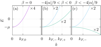
Figure 1: Representative dispersion relations for the spherically symmetric model described by Eq. (17). (a) Without SOC, the bands are fourfold degenerate, and there is a single Fermi surface with wave vector $k_{F,0}=\sqrt{\mu/\alpha}$. Note that we take $\alpha>0$ so that the band has positive effective mass. (b) Turning on the SOC lifts the fourfold degeneracy, yielding two doubly degenerate quadratically dispersing bands with positive effective mass. There are now two Fermi surfaces with wave vectors $k_{F,\pm}=\sqrt{\mu/(\alpha+5\beta/4\pm\beta)}$. (c) For $\beta<-4\alpha/9$, the effective mass of one of the bands becomes negative, and there is only a single Fermi surface.

We start by considering the case of spherically symmetric SOC, i.e., $\beta=\gamma$, and later generalize to the case of cubic anisotropy. In the spherical limit, the normal-state Hamiltonian simplifies to

$$h(\bm{k})=(\alpha\lvert\bm{k}\rvert^{2}-\mu)\,\openone_{4}+\beta(\bm{k}\cdot\bm{J})^{2}.$$ (17)

Representative examples of the normal-state band structure are shown in Fig. 1.

In Fig. 2, we present the phase diagram as a function of temperature and SOC strength. Figures 3(a)–3(f) show the band structure around the Fermi surface in the $[100]$ direction where we anticipate the appearance of nodes from the projected gap in Eq. (12). Any gaps in the spectrum along this direction at nonzero SOC strength are, therefore, due entirely to the interband pairing potential. To obtain comparable results over a wide range of SOC strengths, we fix the critical temperature $T_{c}$ and vary the attractive interaction $V_{0}$ such that the second-order coefficient of the GL free energy vanishes at the chosen $T_{c}$. This eliminates effects due to the changing DOS at the Fermi energy as the SOC is varied.

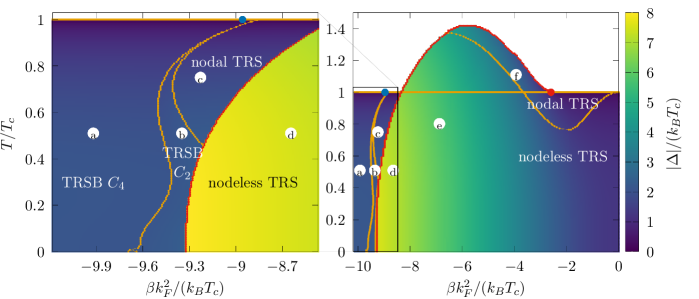
Figure 2: Phase diagram for the $T_{2g}$ pairing states given by Eq. (8) on the SOC-temperature plane. The color code indicates the gap magnitude $\sqrt{\Delta_{xz}^{2}+\Delta_{yz}^{2}}$ where brighter colors mean larger gaps and white means no superconductivity. The horizontal line at $T/T_{c}=1$ denotes the critical temperature $T_{c}$ predicted by GL theory. Lines of first-order (second-order) phase transitions are indicated in red (orange). The blue dot in both panels indicates the point of TRSB from GL theory, the red dot in the panel on the right denotes the onset of the first-order phase transition estimated by GL theory. The left panel is a zoom of the box in the right panel. The SOC strength $\beta$ is plotted as an effective spin-orbit energy $\beta k_{F}^{2}/(k_{B}T_{c})$ where $k_{F}^{2}=\mu/(\alpha+5\beta/4)$.

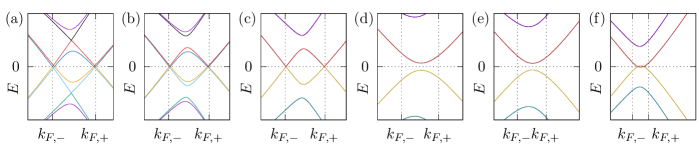
Figure 3: (a)–(f) Band structure in the vicinity of the Fermi energy for parameter sets indicated by the corresponding labels in Fig. 2 along the $[100]$ direction where we expect nodes in a nodal state. The Fermi wave vectors are given by $k_{F,\pm}=\sqrt{\mu/(\alpha+5\beta/4\pm\beta)}$.

Starting at $\beta=0$, we find the fully gapped TRS-preserving state (“nodeless TRS”) predicted by Ho and Yip (1999). Switching on the SOC, we observe that the gap just below the critical temperature has nodes (“nodal TRS”), but the nodeless TRS state is recovered at lower temperatures. The nodal behavior arises as the SOC lifts the fourfold degeneracy of the bands, making a distinction between inter- and intraband pairings possible. Close to the critical temperature, the strength of the pairing potential is much smaller than the band splitting so that the gap at the Fermi surface is controlled by the nodal intraband pairing potential in Eq. (12). However, as the pairing potential grows upon lowering the temperature, the interband potential shifts the nodes away from the Fermi surfaces at $k_{F,\pm}=\sqrt{\mu/(\alpha+5\beta/4\pm\beta)}$ as seen in the band structure at point (f) in Fig. 3. At a critical value of the pairing potential, the nodes meet and annihilate, marking the recovery of the nodeless TRS phase.

A further increase in SOC leads to an enhancement of the critical temperature over the one anticipated from the second-order coefficient of the GL free energy, implying a first-order transition between the normal and the superconducting states. The presence of the first-order phase transition is confirmed by computing the position of the tricritical point from GL theory, i.e., the point where the fourth-order coefficient turns negative. We find very good agreement between the numerical calculation and our GL theory (cf. the red dot in the right panel of Fig. 2). In this region, the magnitude of the pairing potential $\sqrt{\Delta_{xz}^{2}+\Delta_{yz}^{2}}$ is much larger than expected from BCS theory, and the very large interband pairing potentials ensure a full gap as shown by points (d) and (e) in Fig. 2. We, hence, refer to this state as the “large-gap” phase, in contrast to the other, “small-gap” phases. The origin of the first-order phase transition is discussed in Sec. III.2.

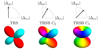
Figure 4: Sketch of the pairing amplitudes $\lvert\Delta_{xz}\rvert$ and $\lvert\Delta_{yz}\rvert$ and of the gap structure in the nodal TRS, TRSB $C_{2}$, and TRSB $C_{4}$ phases, see Fig. 2. The TRSB $C_{2}$ state breaks both TRS and $C_{4}$ symmetry.

Upon increasing the SOC strength beyond $\beta k_{F}^{2}\approx-8.4k_{B}T_{c}$, there is an abrupt drop in the magnitude of the gap, and the nodeless TRS phase gives way to a nodal state. Close to $T_{c}$, this state marked by “nodal TRS” has a gap that is well approximated by Eq. (12) and exhibits line nodes [point (e) in Figs. 2 and 3]. Further below $T_{c}$, we enter a phase which breaks TRS but where the two gap parameters $\Delta_{yz}$ and $\Delta_{xz}$ have unequal magnitude. We label this the “TRSB $C_{2}$” state because the unequal gap magnitudes yield a spectrum with only $C_{2}$ rotational symmetry about the $z$ axis. The magnitudes of $\Delta_{yz}$ and $\Delta_{xz}$ converge as the SOC is increased, thus, realizing the “TRSB $C_{4}$” state where the spectrum has $C_{4}$ rotational symmetry about the $z$ axis. This is the $\bm{l}=(1,i,0)$ state and is consistent with predictions of the strong-SOC limit discussed in Sec. II.2.2. The intermediate TRSB $C_{2}$ state can be visualized as a continuous rotation of the vector $\bm{l}$ from $(1,0,0)$ to $(1,i,0)$, see Fig. 4. The boundary of the TRSB $C_{4}$ phase shows reentrant behavior, but it is realized at all temperatures for $\beta k_{F}^{2}\approx-9.7k_{B}T_{c}$. Both the TRSB $C_{4}$ and the $C_{2}$ phases display BFSs.

The critical value of the SOC strength for which the TRSB state becomes stable just below $T_{c}$ is estimated from an expansion of the GL free energy to fourth order at $\beta k_{F}^{2}\approx-8.957k_{B}T_{c}$. This estimate is shown as the blue dot in both panels of Fig. 2 and is in excellent agreement with the mean-field theory. A previous analysis Agterberg et al. (2017a) had estimated this critical strength to be $\beta k_{F}^{2}\approx-11.572k_{B}T_{c}$ (expressed in our units) and, therefore, overestimated it by about $30\%$. The disagreement stems from the approximate treatment of the band splitting in Ref. Agterberg et al. (2017a). Nevertheless, we confirm that the TRSB state is realized at moderate values of the SOC strength.

III.1 Effects of cubic anisotropy

Cubic anisotropy is introduced in our model by setting $\gamma\neq\beta$ in the Luttinger-Kohn Hamiltonian. In Fig. 5, we show the pairing state realized just below the critical temperature as a function of $\beta$ and the cubic anisotropy parameter $\gamma-\beta$. Note that the transition into the large-gap phase is of first order and the critical temperature, therefore, exceeds the temperature at which the second-order coefficient in the GL expansion changes sign. As can be seen, there is a pronounced asymmetry between the cases of $\lvert\gamma\rvert>\lvert\beta\rvert$ and $\lvert\gamma\rvert<\lvert\beta\rvert$: The region of first-order transitions into the large-gap phase is suppressed for $\lvert\gamma\rvert>\lvert\beta\rvert$ and disappears entirely for sufficiently strong $\gamma$, and the TRSB state occurs at smaller values of the SOC strength $\lvert\beta\rvert$. These trends are reversed for $\gamma>\beta$.

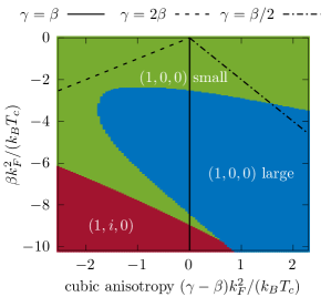
Figure 5: Phase diagram just below the critical temperature as a function of SOC strength and cubic anisotropy. “$(1,0,0)$ small” and “$(1,0,0)$ large” refer to the TRS-preserving phase, whereas “$(1,i,0)$” specifies the TRSB $C_{4}$ phase with BFSs.

In Fig. 6, we show temperature-dependent phase diagrams along two lines $\gamma=2\beta$ and $\gamma=\beta/2$. Along the cut $\gamma=2\beta$, there is no first-order phase transition. The change in gap magnitude along the nodeless to nodal transition is steep but not abrupt. This transition is accompanied by the disappearance of nodes. The intermediate $C_{2}$ phase is also heavily suppressed. Along the other cut $\gamma=\beta/2$, we do not recover the small-gap phase within the boundaries of the graph. Therefore, we also do not observe the point of TRSB as predicted by GL theory.

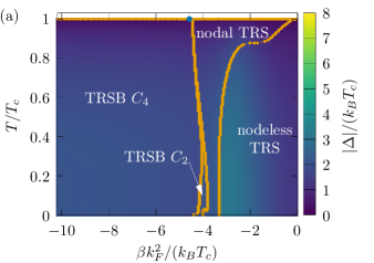
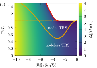
Figure 6: Phase diagrams on the SOC-temperature plane along two lines (a) $\gamma=2\beta$ and (b) $\gamma=\beta/2$. The color code represents the gap magnitude where brighter colors mean larger gaps and white means no superconductivity. Lines of first-order (second-order) phase transitions are indicated in red (orange). For $\gamma=2\beta$, panel (a), there is no first-order phase transition at $T_{c}$. Below $T_{c}$, we find a large-gap phase, but the transition to it is not of first order. For $\gamma=\beta/2$, panel (b), the large-gap phase occurs. The critical temperature is strongly enhanced, and larger gaps are found. In both panels, the blue dot at $T_{c}$ is the point of TRSB, and the red dot at $T_{c}$ is the tricritical point as predicted by the GL free energy.

The phase diagram in Fig. 5 can be understood by looking at the expression for the effective intraband pairing Eq. (12). We find that the magnitude of the intraband pairing is proportional to $\gamma$, i.e., larger (smaller) $\gamma$ means stronger (weaker) intraband pairing compared to interband pairing. The existence of the large-gap phase depends on the ratio between intra- and interband pairings as we will discuss in the next section.

III.2 Origin of the first-order transition

The first-order phase transition into the large-gap phase shown in Figs. 2, 5, and 6 is one of the most surprising features of the phase diagram of our model. The inclusion of cubic anisotropy reveals that it is not generic, however, but rather depends upon the balance between the two spin-orbit terms. In this section, we show that the first-order transition is controlled by the relative strengths of the intra- and interband pairing potentials, which, in turn, depends on the SOC strengths as noted above.

The first-order transition can be understood based on a simplified model with two bands in which we fix the ratio of the inter- and intraband pairing potentials. In this model, the normal-state bands have the dispersions $\xi_{\bm{k},\pm}=(1\pm\delta)\epsilon_{\bm{k}}-\mu$, where $\delta$ parametrizes the band splitting and the precise form of $\epsilon_{\bm{k}}$ is unimportant. The splitting parameter $\delta$ plays a role analogous to the SOC strength in the full model where the band splitting is characterized by differing effective masses of the Luttinger-Kohn bands as illustrated in Fig. 1.

Since the interband and intraband pairing potentials are obtained by projecting $\Delta$ from Eq. (8) into the band basis, the relative strength of the interband and intraband pairing potentials is determined by details of the normal-state band structure. To represent this aspect, we write the pairing potential in the band basis as

$$\Delta=\eta\begin{pmatrix}r&\sqrt{1-r^{2}}\\ \sqrt{1-r^{2}}&-r\\ \end{pmatrix},$$ (18)

where $\eta$ is the magnitude of the pairing potential, and the coefficient $r$ controls the relative strength of intra- and interband pairings: $r=0$ corresponds to pure interband pairing and $r=1$ to pure intraband pairing. The intraband pairing has opposite signs in each band, in agreement with Eq. (12). Since the first-order transition only occurs into a TRS-preserving state, in the following we assume that $r$ and $\eta$ are real. Note that for the pairing potential in Eq. (18), the ratio between intra- and interband pairings is momentum independent. In contrast, in the full model, this quantity varies across the Fermi surface. We can nevertheless define this ratio for the full model in terms of the Fermi-surface average,

$$r^{2}=\frac{1}{\Delta_{xz}^{2}+\Delta_{yz}^{2}}\int\frac{\mathop{}\!\mathrm{d}\Omega}{4\pi}\>\lvert\psi_{\bm{k}}^{\text{intra}}\rvert^{2}.$$ (19)

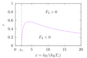
Figure 7: Phase diagram of the simple model as a function of the pairing ratio $r$ and the band splitting $\delta$. In this model, first-order phase transitions are only possible for $x>x_{c}$ because only then there is a region where $F_{4}<0$.

The GL expansion of the free energy of the simple model gives a Taylor series in the parameter $\eta$,

$$F=F_{2}\eta^{2}+F_{4}\eta^{4}+\mathcal{O}(\eta^{6}),$$ (20)

where expressions for the coefficients $F_{2}$ and $F_{4}$ can be obtained from Eqs. (10a) and (10b). A negative sign of the fourth-order coefficient $F_{4}$ indicates that the transition into the superconducting state is of first order. We show the variation of the sign of this coefficient as a function of the parameters $r$ and $\delta$ in Fig. 7. For sufficiently small intraband pairing strength $r$, we find that $F_{4}$ is positive at small band splitting $\delta$, becomes negative for increasing $\delta$, and finally returns to a positive value. Assuming that higher-order terms in the GL expansion can be ignored, this indicates that the phase transition becomes discontinuous beyond a critical band splitting, but a continuous transition is recovered as the band splitting is further increased.

The conclusions for the simple model are broadly in agreement with the phase diagrams for the full model in Figs. 2 and 5. Equation (19) gives $r=1/\sqrt{5}$ for the full model in the spherical limit. According to the simple model, the phase transition at this value of $r$ becomes discontinuous at $\lvert x\rvert=\lvert\delta\mu/(k_{B}T_{c})\rvert\approx 2.460$, which is in very good agreement with the location of the tricritcal point for the full model at $\lvert x\rvert\approx 2.594$ (red dot in Fig. 2) where the effective band splitting is given by $\delta=\beta/(\alpha+5\beta/4)$. The simple model also explains the asymmetric effect of the cubic anisotropy seen in Fig. 5: For $\lvert\gamma\rvert>\lvert\beta\rvert$, the intraband pairing potential is enhanced, which, in turn, increases the value of $r$ and, thus, suppresses the first-order transition. Conversely, $\lvert\gamma\rvert<\lvert\beta\rvert$ reduces the intraband pairing potential and, thus, $r$ and favors the first-order transition.

The simple model and our full results agree in showing that a second-order transition is recovered at sufficiently large values of the band splitting $\delta$. The reappearance of the second-order transition in the full model, however, does not occur with a tricritical point, but rather with a discontinuous jump in the minimum of the free energy from a large value of the gap magnitude $(\Delta_{xz}^{2}+\Delta_{yz}^{2})^{1/2}$ (large-gap phase) to a minimum at a small value of the gap magnitude (small-gap phase). Properly capturing this behavior in the simple model would require extending the GL expansion in Eq. (20) to, at least, eighth order in $\eta$.

IV Properties of the time-reversal-symmetry-breaking state

We now investigate features of the TRSB $C_{4}$ state. We choose the parameter set labeled by (c) in Figs. 2 and 3. In this case, we can set $\Delta_{xz}=\Delta_{yz}=\Delta_{0}$, and so, the pairing potential is $\Delta=\Delta_{0}\,(\eta_{yz}+i\eta_{xz})$.

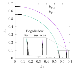
Figure 8: BFSs for the parameters labeled by (c) in Figs. 2 and 3 (heavy black lines). The colored lines denote the normal-state Fermi surfaces of the $+$ and $-$ bands. $k_{\perp}$ is the radial component of the momentum on the $k_{x}k_{y}$-plane.

IV.1 Bogoliubov Fermi surfaces

First, we map out the BFSs by searching for vanishing energy eigenvalues. Thanks to rotational symmetry around the $z$ axis and inversion symmetry, we can restrict ourselves to the first octant. The resulting nodal surfaces are shown in Fig. 8. In the TRSB $C_{4}$ state, the magnitude of the pseudomagnetic field in Eq. (15) is

$$\lvert\bm{h}(\bm{k})\rvert=\frac{4\lvert\Delta_{0}\rvert^{2}}{(\epsilon_{\bm{k},+}-\epsilon_{\bm{k},-})^{2}}\,\beta\,\sqrt{\lvert\bm{k}\rvert^{4}-3(k_{x}^{2}+k_{y}^{2})k_{z}^{2}}.$$ (21)

The size of the BFSs scales with the magnitude of the pseudomagnetic field. Since this field is inversely proportional to the band splitting squared, which grows as $\lvert\bm{k}\rvert^{2}$, the inner BFS is larger than the outer one, see the inset of Fig. 8. The pseudomagnetic field has the largest magnitude close to the boundary with the TRSB $C_{2}$ state since this corresponds to the smallest band splitting for which the TRSB $C_{4}$ state is stable. Here, the BFSs have the largest volume and are, therefore, clearly distinguishable from line and point nodes.

The existence of BFSs leads to a nonzero DOS at zero energy, which is not expected for clean superconductors. We compute the DOS numerically from the mean-field dispersion and analytically using the low-energy dispersion from Eq. (16). In the absence of cubic anisotropy, close to the Fermi surface, $\bm{h}(\bm{k})$, $\gamma_{\bm{k}}$, and $\psi_{\bm{k},\pm}$ only depend upon the polar angle $\theta$. The DOS in the $\pm$ band is, thus,

$$\rho_{\pm}(E)=\mathcal{N}_{0,\pm}\sum_{a,b}\int_{0}^{\pi}\frac{\bigl{|}E-a\lvert\bm{h}_{\pm}(\theta)\rvert\bigr{|}\,\sin\theta\mathop{}\!\mathrm{d}\theta}{\sqrt{(E-a\lvert\bm{h}_{\pm}(\theta)\rvert)^{2}-\lvert\psi_{\pm}(\theta)\rvert^{2}}},$$ (22)

where we have assumed the normal-state DOS $\mathcal{N}_{0,\pm}$ to be constant in the range of the superconducting gap. Evaluating Eq. (22), we find excellent agreement with the numerical results, as shown in Fig. 9. In particular, we clearly see a large residual DOS at zero energy in the superconducting gap of up to 20% of the normal-state DOS. The flat DOS at zero energy results from the lifting of the pseudospin degeneracy by the pseudomagnetic field $\bm{h}$. This shifts the DOS for each pseudospin species, leading to the scaling $\rho(E)\propto(\lvert E+\lvert\bm{h}\rvert\rvert+\lvert E-\lvert\bm{h}\rvert\rvert)/2$ instead of $\rho(E)\propto\lvert E\rvert$, as would be the case for line nodes. This gives a constant DOS for $-\lvert\bm{h}\rvert<E<\lvert\bm{h}\rvert$, as previously reported in Ref. Lapp et al. (2019). The effect of the pseudomagnetic field is also seen in the splitting of the coherence peaks: In the absence of the pseudomagnetic field, we expect a single coherence peak at $\lvert E\rvert=\Delta_{0}$. Upon adding the pseudomagnetic field, it is split into four coherence peaks at $\Delta_{0}+\lvert\bm{h}_{\pm}(\theta=\pi/4)\rvert$ and $\Delta_{0}-\lvert\bm{h}_{\pm}(\theta=\pi/4)\rvert$, where $\theta=\pi/4$ is the angle of maximum gap. Since the pseudomagnetic field has different magnitude at the two Fermi surfaces, these two peaks are, in turn, weakly split.

A residual DOS in an unconventional superconductor can also arise due to the presence of impurities Mineev and Samokhin (1999). We can estimate the required concentration of impurities to achieve a zero-energy residual DOS as large as 20% of the normal-state DOS within the self-consistent Born approximation. Using the exact results for the polar phase of ³He, which also has an equatorial line node, we estimate that the required concentration of impurities would approximately result in a 40% suppression of $T_{c}$ compared to the clean limit. It should be possible to rule out the effect of impurities by considering the residual DOS as a function of $T_{c}$ for different samples. We also emphasize that the splitting of the coherence peaks seen in Fig. 9 cannot be explained by impurity effects.

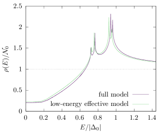
Figure 9: DOS in the superconducting state for the parameters labeled by (c) in Figs. 2 and 3, based on a full two-band calculation (black curve) and on a low-energy single-band approximation (green curve). The results of the two approaches agree very well. The residual DOS at zero energy is as large as 20% of the normal-state DOS at the Fermi energy $\mathcal{N}_{0}=\sqrt{\mu}/2(\alpha+5\beta/4)^{3/2}$.

IV.2 Induced magnetic order parameter

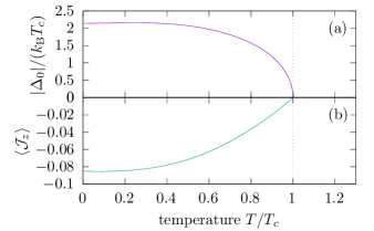
Figure 10: (a) Gap parameter and (b) induced magnetic order parameter as functions of temperature in the TRSB phase and with the SOC labeled by (c) in Figs. 2 and 3.

As pointed out in Ref. Brydon et al. (2018), the pseudomagnetic field can be interpreted as manifesting a subdominant secondary magnetic order parameter, which is induced by the superconductivity. This subdominant order is related to the time-reversal odd part of the gap product,

$$\Delta\Delta^{\dagger}-U_{T}\Delta^{\ast}\Delta^{T}U_{T}^{\dagger}=\frac{4}{3}\,\Delta_{0}^{2}(7J_{z}-4J_{z}^{3})\mathrel{\equiv}2\Delta_{0}^{2}\mathcal{J}_{z}.$$ (23)

In Fig. 10, we show the expectation value of $\mathcal{J}_{z}$ together with the superconducting gap as functions of temperature. The superconductivity and magnetism appear together but their temperature dependence close to the critical temperature is notably different: whereas the gap magnitude scales as $\Delta_{0}\sim\lvert T-T_{c}\rvert^{1/2}$, the expectation value of $\mathcal{J}_{z}$ scales as $\mathinner{\langle\mathcal{J}_{z}\rangle}\sim\lvert T-T_{c}\rvert$. This linear temperature dependence close to $T_{c}$ reflects its relation to the gap product in Eq. (23).

The finite expectation value of $\mathcal{J}_{z}$ generically leads to a finite pseudomagnetic field in Eq. (15) and, thus, to a momentum-dependent spin polarization. To understand the interplay between magnetism and superconductivity, we include a magnetic order parameter $m_{z}$ in the channel that couples to superconductivity in the GL expansion. To that end, following Dahl and Sudbø (2007), we redefine:

$$\Sigma=\begin{pmatrix}\mathcal{M}_{z}&\Delta\\ \Delta^{\dagger}&-\mathcal{M}_{z}^{T}\\ \end{pmatrix},$$ (24)

in Eq. (10b), where $\mathcal{M}_{z}=m_{z}\mathcal{J}_{z}$. The lowest-order coupling between the superconducting and magnetic order parameters occurs at third order and has the form

$$iF_{3}m_{z}(\Delta_{xz}\Delta_{yz}^{*}-\Delta_{xz}^{*}\Delta_{yz}),$$ (25)

which clearly indicates that the TRSB superconducting state induces the magnetism. The lengthy expression for the coefficient $F_{3}$ is presented in Appendix B. In particular, we must introduce a cutoff $\Lambda$ of the attractive pairing interaction to account for particle-hole asymmetry in the normal state. In the limit where the band splitting and cutoff are much larger than $k_{B}T_{c}$ (i.e., the conditions under which the TRSB state is stable), the coefficient simplifies to

$$F_{3}=\frac{\mathcal{N}_{0}}{\mu}\,\frac{48}{5}\biggl{[}1-\frac{\ln\frac{2\Lambda e^{\gamma}}{\pi k_{B}T_{c}}}{3(1-\tilde{\beta}^{2})}-\frac{1}{4}\ln\biggl{(}1+\frac{\Lambda^{2}}{\tilde{\beta}^{2}\mu^{2}}\biggr{)}\biggr{]},$$ (26)

where $\mathcal{N}_{0}=\sqrt{\mu}/2\,(\alpha+5\beta/4)^{3/2}$ is the normal-state DOS at the Fermi energy, $\tilde{\beta}=\beta/(\alpha+5\beta/4)$, $\tilde{\beta}\mu$ is the band splitting, and $\gamma$ is the Euler-Mascheroni constant. To understand this result, we note that the magnetic order paramater $m_{z}$ couples to $\mathcal{J}_{z}$, which is not diagonal in the band basis but has both interband and intraband components. The intraband component directly couples to the pseudomagnetic field generated by the interband pairing potentials and gives a cutoff-independent contribution to $F_{3}$. On the other hand, the interband components of the magnetic order couple to both the intraband and the interband pairing potentials and give the cutoff-dependent contribution, see Appendix B for details. These two contributions have opposite signs and the contribution from the interband component is likely dominant when $\Lambda\gg k_{B}T_{c}$.

It is interesting to compare our results to the more familiar case of coupling between ferromagnetic and superconducting order parameters in a single-band TRSB superconductor Mineev and Samokhin (1999). A similar GL expansion of the free energy in that case also gives a third-order coupling term with coefficient proportional to $\mathcal{N}_{0}/\mu$, which implies that the magnetization in the superconducting state is on the order of $\Delta_{0}^{2}/\mu^{2}$ and is, hence, expected to be weak. This property is thought to be generic for TRSB superconductors Cross (1975); Mermin and Muzikar (1980). In the present case, it can be understood as being due to the fact that the $j=1/2$ and $j=-3/2$ quasiparticles do not participate in the pairing. The spin of these unpaired quasiparticles then compensates the polarization of the Cooper pairs as is the case for a spin-$1/2$ superconductor where only the up spin is paired and the unpaired down spin compensates the polarization Mineev and Samokhin (1999). The presence of a BFS, therefore, does not imply a strong magnetization of the superconductor.

V Summary and conclusions

In this paper, we have used BCS mean-field theory to study the evolution of the quintet superconducting state in the paradigmatic Luttinger-Kohn model as a function of the SOC strength. We find a rich phase diagram in the SOC-temperature plane. For weak SOC, a time-reversal-symmetric superconducting state is realized. Upon increasing the SOC strength, the transition into the superconducting state becomes first order. The origin of the first-order transition is the competition between inter- and intraband pairings, which is controlled by the cubic anisotropy of the SOC; for sufficiently anisotropic SOC, the first-order transition can be completely suppressed. Upon further increasing the SOC strength, first a second-order transition is recovered, and finally a TRSB pairing state is stabilized. At low temperatures, the TRSB state displays reentrant behavior as well as a first-order transition into the TRS-preserving state.

The TRSB state exhibits BFSs and a residual DOS at the Fermi energy, which can be as large as 20% of the normal-state DOS. The TRSB pairing state induces a subdominant magnetic order parameter, which we find to be small even if the residual DOS is sizable, consistent with the general result that TRSB superconductors have weak intrinsic magnetization.

Our analysis establishes that a pairing state with BFSs can be thermodynamically stable, even when the residual DOS at the Fermi energy due to the BFSs is a sizable fraction of the normal-state DOS. This result is encouraging for experimental searches for BFSs as it shows that the residual DOS due to the BFSs can be of detectable magnitude. Since the size of the BFSs is controlled by the ratio of the interband pairing potential to the band splitting, materials where this ratio is as large as possible are the best candidates. This suggests that heavy-fermion superconductors are promising. It is, therefore, intriguing that a residual DOS has been observed in URu₂Si₂ Kasahara et al. (2007) and UTe₂ Ran et al. (2019); Metz et al. (2019).

Appendix A Evaluation of the Ginzburg-Landau free energy

The GL free energy in Eq. (10) can be evaluated analytically using natural approximations. For a single-band superconductor, it is usually assumed that the DOS at the Fermi energy is constant such that the sum over momenta in Eq. (10a) can be recast into an integral over energy. We adapt this method to our two-band model by rewriting the eigenenergies in Eq. (II) in terms of an “unsplit” dispersion $\epsilon_{0}(\bm{k})$ and a cubic form factor $f(\hat{\bm{k}})$ with unit vector $\hat{\bm{k}}$,

$$\epsilon_{\bm{k},\pm}=\biggl{(}1\pm\frac{f(\hat{\bm{k}})}{\alpha+5\beta/4}\biggr{)}\,\epsilon_{0}(\bm{k})\pm\frac{f(\hat{\bm{k}})}{\alpha+5\beta/4}\,\mu,$$ (27)

where

$$\epsilon_{0}(\bm{k}) =\biggl{(}\alpha+\frac{5\beta}{4}\biggr{)}\,\lvert\bm{k}\rvert^{2}-\mu,$$ (28)

$$f(\hat{\bm{k}}) =\frac{\beta}{\lvert\bm{k}\rvert^{2}}\sqrt{\sum_{i}\biggl{[}k_{i}^{4}+\biggl{(}\frac{3\gamma^{2}}{\beta^{2}}-1\biggr{)}k_{i}^{2}k_{i+1}^{2}\biggr{]}}.$$ (29)

In the spherical limit $\beta=\gamma$, the form factor reduces to $f(\theta,\phi)=\beta$, which is angle independent. Then, assuming constant normal-state DOS, we make the replacement,

$$\sum_{\bm{k}}\to\mathcal{N}_{0}\int_{\mathbb{S}_{2}}\frac{\mathop{}\!\mathrm{d}\Omega}{4\pi}\int_{-\infty}^{\infty}\mathop{}\!\mathrm{d}\epsilon_{0},$$ (30)

where $\mathcal{N}_{0}=\sqrt{\mu}/2\,(\alpha+5\beta/4)^{3/2}$ is the “unsplit” normal-state DOS at the Fermi energy.

In the case of the fourth-order term, the integral over energy $\epsilon_{0}$ and the following summation over $i\omega_{n}$ results in a sum of polygamma functions which does not yield particular insight and is not reproduced here. Nevertheless, below we demonstrate how to obtain GL coefficients with the outlined approach for the example of the lowest-order coupling between the superconducting and the magnetic order parameters.

Appendix B Third-order term

Figure 11: General form of the diagrams that are generated by the third-order term of the GL free energy. Note that $\mathcal{M}_{z}$ always connects two lines of the same kind, whereas $\Delta$ connects to one particle- and one holelike line.

In this appendix, we outline the derivation of the leading term in the GL expansion that couples the superconducting and magnetic order parameters. In the spherical limit $\beta=\gamma$, the Green’s functions of the particlelike and holelike excitations of the normal state have the explicit forms

$$G_{0}(\bm{k},i\omega_{n}) =\sum_{\pm}G_{\pm}\,\frac{1\pm[(\hat{\bm{k}}\cdot\bm{J})^{2}-5/4]}{2},$$ (31)

$$\tilde{G}_{0}(\bm{k},i\omega_{n}) =\sum_{\pm}\tilde{G}_{\pm}\,\frac{1\pm[(\hat{\bm{k}}\cdot\bm{J}^{T})^{2}-5/4]}{2},$$ (32)

where unit matrices have been suppressed and we have introduced the single-band Green’s functions,

$$G_{\pm} \equiv\frac{1}{i\omega_{n}-\epsilon_{\bm{k},\pm}},$$ (33)

$$\tilde{G}_{\pm} \equiv\frac{1}{i\omega_{n}+\epsilon_{\bm{k},\pm}}.$$ (34)

The magnetic and superconducting order parameters are given by

$$\mathcal{M}_{z} =\frac{2}{3}\,m_{z}(7J_{z}-4J_{z}^{3}),$$ (35)

$$\Delta =\Delta_{0}(\eta_{yz}+i\eta_{xz}),$$ (36)

respectively, and are arranged in the matrix $\Sigma$ as shown in Eq. (24). With these definitions, the trace in the third-order coefficient can be expanded in products of $G_{\pm}$ and $\tilde{G}_{\pm}$. We denote this product without the prefactors as $F_{3}$ such that

$$k_{B}T\sum_{\bm{k},\omega_{n}}\frac{1}{3}\operatorname{Tr}[(G\Sigma)^{3}]=F_{3}m_{z}\lvert\Delta_{0}\rvert^{2}.$$ (37)

Figure 11 shows the general diagrammatic form of the generated term for which there are 12 possibilities. However, four of these have vanishing coefficients so that only eight terms remain in two groups of four,

$$F_{3} =k_{B}T\sum_{\bm{k},\omega_{n}}\{6\sin^{2}(2\theta)(-G_{-}\tilde{G}_{-}G_{+}-G_{-}G_{+}\tilde{G}_{+}+\tilde{G}_{-}G_{+}\tilde{G}_{+}+G_{-}\tilde{G}_{-}\tilde{G}_{+})$$

$$\quad{}+[5+3\cos(4\theta)](-\tilde{G}_{-}G_{+}G_{+}+G_{-}\tilde{G}_{+}\tilde{G}_{+}+\tilde{G}_{-}\tilde{G}_{-}G_{+}-G_{-}G_{-}\tilde{G}_{+})\},$$ (38)

where $\theta$ is the polar spherical angle of $\bm{k}$. There is no contribution where the Green’s functions all have the same band index, which shows that the coupling to the magnetic order parameter requires interband pairing. The combination of Green’s functions appearing in the first line couples the interband component of the magnetic order parameter to one interband and one intraband component of the superconducting pairing potential. On the other hand, the combination of Green’s functions in the second line couples the intraband component of the magnetic order parameter to two interband components of the superconducting order. The latter terms correspond to the coupling of the magnetic order parameter with the pseudomagnetic field in the low-energy effective model. Using the approximation from Eq. (30), we find that only this term gives a nonzero contribution,

$$k_{B}T\sum_{\omega_{n}}\int_{-\infty}^{\infty}\mathop{}\!\mathrm{d}\epsilon_{0}\bigl{(}-G_{-}\tilde{G}_{-}G_{+}-G_{-}G_{+}\tilde{G}_{+}+\tilde{G}_{-}G_{+}\tilde{G}_{+}+G_{-}\tilde{G}_{-}\tilde{G}_{+}\bigr{)} =0,$$ (39)

$$k_{B}T\sum_{\omega_{n}}\int_{-\infty}^{\infty}\mathop{}\!\mathrm{d}\epsilon_{0}\bigl{(}-\tilde{G}_{-}G_{+}G_{+}+G_{-}\tilde{G}_{+}\tilde{G}_{+}+\tilde{G}_{-}\tilde{G}_{-}G_{+}-G_{-}G_{-}\tilde{G}_{+}\bigr{)} =-\frac{1}{\pi k_{B}T_{c}}\,\tilde{\beta}\,\operatorname{Im}\biggl{[}\psi^{(1)}\biggl{(}\frac{1}{2}+\frac{i\tilde{\beta}\mu}{2k_{B}T_{c}\pi}\biggr{)}\biggr{]},$$ (40)

where $\psi^{(n)}(z)$ is the polygamma function of order $n$ and $\tilde{\beta}=\beta/(\alpha+5\beta/4)$. Performing the angular integration, we obtain

$$F_{3} =-\mathcal{N}_{0}\,\frac{24}{\pi k_{B}T_{c}}\,g_{M}\lvert\Delta_{0}\rvert^{2}\tilde{\beta}\operatorname{Im}\biggl{[}\psi^{(1)}\biggl{(}\frac{1}{2}+\frac{i\tilde{\beta}\mu}{2\pi k_{B}T_{c}}\biggr{)}\biggr{]}$$

$$\approx\frac{\mathcal{N}_{0}}{\mu}\,\frac{48}{5}\,g_{M}\lvert\Delta_{0}\rvert^{2},$$ (41)

where the last approximation is valid when the band splitting $\tilde{\beta}\mu$ is much larger than $k_{B}T_{c}$.

The coefficient $F_{3}$ is on the order of $\mathcal{N}_{0}/\mu\approx\mathcal{N}_{0}^{\prime}$, i.e., the derivative of the DOS at the Fermi energy. This suggests that we should also include the contributions due to the particle-hole asymmetry of the normal-state electronic structure, which should also be proportional to the derivative of the DOS. To this end, we expand the DOS up to first order in energy, $\mathcal{N}(\epsilon_{0})\mathrel{\approx}\mathcal{N}_{0}\,[1+\epsilon_{0}/(2\mu)]$. We have already evaluated the contribution of the constant term; including the energy-dependent term, however, typically leads to the divergence of the Matsubara sum. We, therefore, introduce an energy cutoff such that the sum is restricted to $\lvert\omega_{n}\rvert<\Lambda$ where $\Lambda$ is the cutoff energy of the attractive pairing interaction Coleman (2015). Evaluating the different sets of Green’s functions in Eq. (B), we obtain

$$k_{B}T\sum_{\lvert\omega_{n}\rvert<\Lambda}\int_{-\infty}^{\infty}\mathop{}\!\mathrm{d}\epsilon_{0}\>\frac{\epsilon_{0}}{2\mu}\,\bigl{(}-G_{-}\tilde{G}_{-}G_{+}-G_{-}G_{+}\tilde{G}_{+}+\tilde{G}_{-}G_{+}\tilde{G}_{+}+G_{-}\tilde{G}_{-}\tilde{G}_{+}\bigr{)}=-\frac{H_{{\frac{\Lambda}{2k_{B}T\pi}}}+\ln 4}{\mu(1-\tilde{\beta}^{2})},$$ (42)

$$k_{B}T\sum_{\lvert\omega_{n}\rvert<\Lambda}\int_{-\infty}^{\infty}\mathop{}\!\mathrm{d}\epsilon_{0}\>\frac{\epsilon_{0}}{2\mu}\,\bigl{(}-\tilde{G}_{-}G_{+}G_{+}+G_{-}\tilde{G}_{+}\tilde{G}_{+}+\tilde{G}_{-}\tilde{G}_{-}G_{+}-G_{-}G_{-}\tilde{G}_{+}\bigr{)}$$

$$\quad=\frac{1}{2\mu}\left(2\operatorname{Re}\left[H_{-\frac{1}{2}+\frac{i\tilde{\beta}\mu}{2k_{B}T\pi}}\right]-2\operatorname{Re}\left[H_{\frac{i\tilde{\beta}\mu+\Lambda}{2k_{B}T\pi}}\right]\right),$$ (43)

where $H_{z}$ is the analytic continuation of the harmonic number. Combining these results with the contribution of the constant-DOS term, we obtain

$$F_{3} =\mathcal{N}_{0}g_{M}\lvert\Delta_{0}\rvert^{2}\,\frac{24}{5\pi}\,\biggl{\{}-\frac{\tilde{\beta}}{k_{B}T_{c}}\operatorname{Im}\biggl{[}\psi^{(1)}\biggl{(}\frac{1}{2}+\frac{i\tilde{\beta}\mu}{2\pi k_{B}T_{c}}\biggr{)}\biggr{]}-\frac{2\pi}{3}\,\frac{H_{\frac{\Lambda}{2k_{B}T_{c}\pi}}+\ln 4}{\mu(1-\tilde{\beta}^{2})}+\frac{\pi}{\mu}\operatorname{Re}\left[H_{-\frac{1}{2}+\frac{i\tilde{\beta}\mu}{2k_{B}T_{c}\pi}}-H_{\frac{i\tilde{\beta}\mu+\Lambda}{2k_{B}T_{c}\pi}}\right]\biggr{\}}$$

$$\approx g_{M}\,\frac{\mathcal{N}_{0}}{\mu}\,\frac{48}{5}\left[1-\frac{\ln\frac{2\Lambda e^{\gamma}}{\pi k_{B}T_{c}}}{3(1-\tilde{\beta}^{2})}-\frac{1}{4}\ln\left(1+\frac{\Lambda^{2}}{\tilde{\beta}^{2}\mu^{2}}\right)\right],$$ (44)

where the second line is valid in the limit $\Lambda$, $\tilde{\beta}\mu\gg k_{B}T_{c}$ and $\gamma$ is the Euler-Mascheroni constant.

References

- Mineev and Samokhin (1999) V. P. Mineev and K. V. Samokhin, Introduction to Unconventional Superconductivity (Gordon and Breach Science Publishers, New York, 1999).
- Agterberg et al. (2017a) D. F. Agterberg, P. M. R. Brydon, and C. Timm, “Bogoliubov Fermi surfaces in superconductors with broken time-reversal symmetry,” Phys. Rev. Lett. 118, 127001 (2017a).
- Brydon et al. (2018) P. M. R. Brydon, D. F. Agterberg, H. Menke, and C. Timm, “Bogoliubov Fermi surfaces: General theory, magnetic order, and topology,” Phys. Rev. B 98, 224509 (2018).
- Kobayashi et al. (2014) S. Kobayashi, K. Shiozaki, Y. Tanaka, and M. Sato, “Topological Blount’s theorem of odd-parity superconductors,” Phys. Rev. B 90, 024516 (2014).
- Zhao et al. (2016) Y. X. Zhao, Andreas P. Schnyder, and Z. D. Wang, “Unified theory of and invariant topological metals and nodal superconductors,” Phys. Rev. Lett. 116, 156402 (2016).
- Bzdušek and Sigrist (2017) T. Bzdušek and M. Sigrist, “Robust doubly charged nodal lines and nodal surfaces in centrosymmetric systems,” Phys. Rev. B 96, 155105 (2017).
- Nomoto et al. (2016) T. Nomoto, K. Hattori, and H. Ikeda, “Classification of “multipole” superconductivity in multiorbital systems and its implications,” Phys. Rev. B 94, 174513 (2016).
- Cheung and Agterberg (2019) A. K. C. Cheung and D. F. Agterberg, “Superconductivity in the presence of spin-orbit interactions stabilized by Hund coupling,” Phys. Rev. B 99, 024516 (2019).
- Gao et al. (2010) Y. Gao, W.-P. Su, and J.-X. Zhu, “Interorbital pairing and its physical consequences for iron pnictide superconductors,” Phys. Rev. B 81, 104504 (2010).
- Nicholson et al. (2012) A. Nicholson, W. Ge, J. Riera, M. Daghofer, A. Moreo, and E. Dagotto, “Pairing symmetries of a hole-doped extended two-orbital model for the pnictides,” Phys. Rev. B 85, 024532 (2012).
- Ong et al. (2016) T. Ong, P. Coleman, and J. Schmalian, “Concealed -wave pairs in the condensate of iron-based superconductors,” PNAS 113, 5486–5491 (2016).
- Vafek and Chubukov (2017) O. Vafek and A. V. Chubukov, “Hund interaction, spin-orbit coupling, and the mechanism of superconductivity in strongly hole-doped iron pnictides,” Phys. Rev. Lett. 118, 087003 (2017).
- Agterberg et al. (2017b) D. F. Agterberg, T. Shishidou, J. O’Halloran, P. M. R. Brydon, and M. Weinert, “Resilient nodeless -wave superconductivity in monolayer FeSe,” Phys. Rev. Lett. 119, 267001 (2017b).
- Setty et al. (2019) C. Setty, S. Bhattacharyya, A. Kreisel, and P. Hirschfeld, “Ultranodal pair states in iron-based superconductors,” (2019), arXiv:1903.00481 .
- Hu et al. (2019) L.-H. Hu, P. D. Johnson, and C. Wu, “Pairing symmetry and topological surface state in iron-chalcogenide superconductors,” (2019), arXiv:1906.01754 .
- Fu (2014) L. Fu, “Odd-parity topological superconductor with nematic order: Application to CuxBi2Se3,” Phys. Rev. B 90, 100509(R) (2014).
- Brydon et al. (2016) P. M. R. Brydon, L. Wang, M. Weinert, and D. F. Agterberg, “Pairing of fermions in half-Heusler superconductors,” Phys. Rev. Lett. 116, 177001 (2016).
- Savary et al. (2017) L. Savary, J. Ruhman, J. W. F. Venderbos, L. Fu, and P. A. Lee, “Superconductivity in three-dimensional spin-orbit coupled semimetals,” Phys. Rev. B 96, 214514 (2017).
- Yang et al. (2017) W. Yang, T. Xiang, and C. Wu, “Majorana surface modes of nodal topological pairings in spin- semimetals,” Phys. Rev. B 96, 144514 (2017).
- Roy et al. (2019) B. Roy, S. A. A. Ghorashi, M. S. Foster, and A. H. Nevidomskyy, “Topological superconductivity of spin- carriers in a three-dimensional doped Luttinger semimetal,” Phys. Rev. B 99, 054505 (2019).
- Timm et al. (2017) C. Timm, A. P. Schnyder, D. F. Agterberg, and P. M. R. Brydon, “Inflated nodes and surface states in superconducting half-Heusler compounds,” Phys. Rev. B 96, 094526 (2017).
- Boettcher and Herbut (2018a) I. Boettcher and I. F. Herbut, “Unconventional superconductivity in Luttinger semimetals: Theory of complex tensor order and the emergence of the uniaxial nematic state,” Phys. Rev. Lett. 120, 057002 (2018a).
- Boettcher and Herbut (2018b) I. Boettcher and I. F. Herbut, “Critical phenomena at the complex tensor ordering phase transition,” Phys. Rev. B 97, 064504 (2018b).
- Kim et al. (2018) H. Kim, K. Wang, Y. Nakajima, R. Hu, S. Ziemak, P. Syers, L. Wang, H. Hodovanets, J. D. Denlinger, P. M. R. Brydon, D. F. Agterberg, M. A. Tanatar, R. Prozorov, and J. Paglione, “Beyond triplet: Unconventional superconductivity in a spin- topological semimetal,” Sci. Adv. 4, eaao4513 (2018).
- Kawakami et al. (2018) T. Kawakami, T. Okamura, S. Kobayashi, and M. Sato, “Topological crystalline materials of electrons: Antiperovskites, Dirac points, and high winding topological superconductivity,” Phys. Rev. X 8, 041026 (2018).
- Taylor and Kallin (2012) E. Taylor and C. Kallin, “Intrinsic Hall effect in a multiband chiral superconductor in the absence of an external magnetic field,” Phys. Rev. Lett. 108, 157001 (2012).
- Nomoto and Ikeda (2016) T. Nomoto and H. Ikeda, “Exotic multigap structure in UPt3 unveiled by a first-principles analysis,” Phys. Rev. Lett. 117, 217002 (2016).
- Yanase (2016) Y. Yanase, “Nonsymmorphic Weyl superconductivity in UPt3 based on representation,” Phys. Rev. B 94, 174502 (2016).
- Oiwa et al. (2018) R. Oiwa, Y. Yanagi, and H. Kusunose, “Theory of superconductivity in hole-doped monolayer ,” Phys. Rev. B 98, 064509 (2018).
- Möckli and Khodas (2018) D. Möckli and M. Khodas, “Robust parity-mixed superconductivity in disordered monolayer transition metal dichalcogenides,” Phys. Rev. B 98, 144518 (2018).
- Guo et al. (2018) H. Guo, X. Zhu, S. Feng, and R. T. Scalettar, “Pairing symmetry of interacting fermions on a twisted bilayer graphene superlattice,” Phys. Rev. B 97, 235453 (2018).
- Su and Lin (2018) Y. Su and S.-Z. Lin, “Pairing symmetry and spontaneous vortex-antivortex lattice in superconducting twisted-bilayer graphene: Bogoliubov-de Gennes approach,” Phys. Rev. B 98, 195101 (2018).
- Wu (2019) F. Wu, “Topological chiral superconductivity with spontaneous vortices and supercurrent in twisted bilayer graphene,” Phys. Rev. B 99, 195114 (2019).
- Sigrist and Ueda (1991) M. Sigrist and K. Ueda, “Phenomenological theory of unconventional superconductivity,” Rev. Mod. Phys. 63, 239 (1991).
- Lapp et al. (2019) C. J. Lapp, G. Börner, and C. Timm, “Experimental consequences of Bogoliubov Fermi surfaces,” (2019), arXiv:1909.10370 .
- Luttinger and Kohn (1955) J. M. Luttinger and W. Kohn, “Motion of electrons and holes in perturbed periodic fields,” Phys. Rev. 97, 869 (1955).
- Ho and Yip (1999) T.-L. Ho and S. Yip, “Pairing of fermions with arbitrary spin,” Phys. Rev. Lett. 82, 247 (1999).
- Boettcher and Herbut (2016) I. Boettcher and I. F. Herbut, “Superconducting quantum criticality in three-dimensional Luttinger semimetals,” Phys. Rev. B 93, 205138 (2016).
- Venderbos et al. (2018) J. W. F. Venderbos, L. Savary, J. Ruhman, P. A. Lee, and L. Fu, “Pairing states of spin- fermions: Symmetry-enforced topological gap functions,” Phys. Rev. X 8, 011029 (2018).
- Sim et al. (2019) G. B. Sim, A. Mishra, M. J. Park, Y. B. Kim, G. Y. Cho, and S. B. Lee, “Topological wave superconductors in a multiorbital quadratic band touching system,” Phys. Rev. B 100, 064509 (2019).
- Kasahara et al. (2007) Y. Kasahara, T. Iwasawa, H. Shishido, T. Shibauchi, K. Behnia, Y. Haga, T. D. Matsuda, Y. Onuki, M. Sigrist, and Y. Matsuda, “Exotic superconducting properties in the electron-hole-compensated heavy-fermion “semimetal” URu2Si2,” Phys. Rev. Lett. 99, 116402 (2007).
- Herbut et al. (2019) I. F. Herbut, I. Boettcher, and S. Mandal, “Ground state of the three-dimensional BCS -wave superconductor,” Phys. Rev. B 100, 104503 (2019).
- Dahl and Sudbø (2007) E. K. Dahl and A. Sudbø, “Derivation of the Ginzburg-Landau equations for a ferromagnetic -wave superconductor,” Phys. Rev. B 75, 144504 (2007).
- Cross (1975) M. C. Cross, “A generalized Ginzburg-Landau approach to the superfluidity of helium 3,” J. Low Temp. Phys. 21, 525 (1975).
- Mermin and Muzikar (1980) N. D. Mermin and P. Muzikar, “Cooper pairs versus Bose condensed molecules: The ground-state current in superfluid -,” Phys. Rev. B 21, 980 (1980).
- Ran et al. (2019) S. Ran, C. Eckberg, Q.-P. Ding, Y. Furukawa, T. Metz, S. R. Saha, I-L. Liu, M. Zic, H. Kim, J. Paglione, and N. P. Butch, “Nearly ferromagnetic spin-triplet superconductivity,” Science 365, 684–687 (2019).
- Metz et al. (2019) T. Metz, S. Bae, S. Ran, I-L. Liu, Y. S. Eo, W. T. Fuhrman, D. F. Agterberg, S. Anlage, N. P. Butch, and J. Paglione, “Point node gap structure of spin-triplet superconductor UTe2,” (2019), arXiv:1908.01069 .
- Coleman (2015) P. Coleman, Introduction to Many-Body Physics (Cambridge University Press, Cambridge, U.K., 2015).