Hierarchy of double-time correlations

Abstract

The hierarchy of correlations is an analytical approximation method which allows us to study non-equilibrium phenomena in strongly interacting quantum many-body systems on lattices in higher dimensions. So far, this method was restricted to equal-time correlators $\langle\hat{A}_{\mu}(t)\hat{B}_{\nu}(t)\rangle$. In this work, we generalize this method to double-time correlators $\langle\hat{A}_{\mu}(t)\hat{B}_{\nu}(t^{\prime})\rangle$, which allows us to study effective light cones and Green functions and to incorporate finite initial temperatures.

I Introduction

The physics of strongly interacting quantum many-body systems is, despite decades of research, far from being fully understood. Apart from a few exactly solvable models, even their ground state properties are a subject of ongoing discussions, see, e.g., L04 ; YJNIHY03 . Even more challenging is the investigation of non-equilibrium properties of those interacting many-body systems.

In the limit of infinite dimensions, the Dynamical Mean-field Theory (DMFT) has been successfully applied to various problems such as the Mott-Hubbard transition RZK92 ; RKZ94 ; GK92 ; GKKR96 ; AGPTW10 ; AGPTW11 or the non-equilibrium dynamics in Mott insulators EKW09 ; ATE14 ; EKW10 ; WTE12 ; CWE14 ; FT06 by mapping the system to an effective single site (i.e., zero-dimensional) problem.

Furthermore, one-dimensional strongly interacting systems have been studied by employing exact diagonalization, see, e.g., K16 ; LHS88 ; KLA07 ; KTEG08 ; RB04 , time-dependent Density Matrix Renomalization Group variational techniques (t-DMRG), see, e.g., DKSV04 ; S11 ; WF04 , or Jordan-Wigner transformations JW28 ; LP75 ; BO01 ; BKOSV04 . Moreover, exact analytical solutions were used to study non-equilibrium dynamics D05 and ground state properties. However, the findings for one-dimensional systems cannot be easily transferred to higher dimensions. For example, thermalization in higher dimensions is very different from thermalization in one dimension since for the latter the energy re-distribution cannot occur via two-body collisions (due to energy and momenta conservation).

For strongly interacting systems in higher dimensions, the methods described above run into difficulties. For example, the generalization of t-DMRG to higher dimensions (such as tensor networks) is limited by the exponential scaling with the system width CV09 , especially if correlations spread across the system. For a very similar reason (exponential scaling of Hilbert space), the method of exact diagonalization is limited to small system sizes K16 . On the other hand, the DMFT is only well understood in the limit of infinite dimensions and, due to the mapping to an effective single-site problem, does not capture energy and momentum transfer of quasi-particles or long-range correlations WEFWBH18 .

In order to bridge this gap, we established over the last years a perturbative hierarchical method which is valid for large coordination numbers $Z\gg 1$. This method allows for a systematic study of non-equilibrium properties in strongly interacting systems in large (but finite) dimensions NS10 ; QNS12 ; QKNS14 ; KNQS14 ; NQS14 ; NQS16 ; QS19 ; QS19a .

The hierarchical expansion is based on a controlled expansion of the $n$-point reduced density matrices into correlated parts. At zeroth order in our expansion, we have the single-site density matrix,

$$\hat{\rho}_{\mu}=\mathrm{Tr}_{\not{\mu}}\{\hat{\rho}\}=\mathcal{O}(Z^{0})\,,$$ (1)

where $\mathrm{Tr}_{\not{\mu}}$ denotes the trace over all lattice sites but $\mu$. The correlated part of the two-site density matrix,

$$\hat{\rho}^{\mathrm{corr}}_{\mu\nu}=\mathrm{Tr}_{\not{\mu}\not{\nu}}\{\hat{\rho}\}-\hat{\rho}_{\mu}\hat{\rho}_{\nu}\,,$$ (2)

is of order $\mathcal{O}(1/Z)$, the three-point correlator

$$\hat{\rho}^{\mathrm{corr}}_{\mu\nu\lambda}=\mathrm{Tr}_{\not{\mu}\not{\nu}\not{\lambda}}\{\hat{\rho}\}-\hat{\rho}^{\mathrm{corr}}_{\mu\nu}\hat{\rho}_{\lambda}-\hat{\rho}_{\mu\lambda}^{\mathrm{corr}}\hat{\rho}_{\nu}-\hat{\rho}_{\nu\lambda}^{\mathrm{corr}}\hat{\rho}_{\lambda}-\hat{\rho}_{\mu}\hat{\rho}_{\nu}\hat{\rho}_{\lambda}$$ (3)

is of order $\mathcal{O}(1/Z^{2})$, and so on. The time-evolution of the $n$-point correlations is derived directly from the von Neumann equations. With this expansion, we were able to study quenches across phase boundaries NS10 , ground state properties and non-equilibrium dynamics of quantum correlations in the bosonic and fermionic Hubbard model QKNS14 ; KNQS14 . Although the perturbative scheme is set up for $Z\gg 1$, we found even qualitative agreement with exact diagonalization in one dimension KNQS14 .

The derivation of the hierarchy was based on the real-time evolution of the system’s density matrix. In the following, we shall extend our hierarchical approach to double-time correlation functions. As a concrete example, we will apply the method to the Bose-Hubbard model in the Mott insulating phase. In section II we derive the equations of motion up to order $\mathcal{O}(1/Z)$. A general proof of the hierarchy is given in the Appendix. In section III, we show how Green functions and finite temperature correlation functions are related to the hierarichal equations. In section IV we study the non-equilibrium dynamics at finite temperatures and in section V we derive the double-time correlation functions for a quantum quench of the Bose-Hubbard model.

II The Double-Time Hierarchy

The lattice system under consideration is described by the Bose-Hubbard Hamiltonian ($\hbar=1$)

$$\hat{H}=-\frac{J(t)}{Z}\sum_{\mu,\nu}T_{\mu\nu}\hat{b}^{\dagger}_{\mu}\hat{b}_{\nu}+\sum_{\mu}\left[\frac{U}{2}\hat{n}_{\mu}(\hat{n}_{\mu}-1)-\mu_{0}\hat{n}_{\mu}\right]\,,$$ (4)

where $\hat{b}_{\mu}^{\dagger}$ and $\hat{b}_{\nu}$ are the bosonic creation and annihilation operators at the lattice sites $\mu$ and $\nu$, respectively. The time-dependent hopping rate is denoted by $J(t)$, where we have factored out the coordination number $Z$. The second term describes the on-site repulsion $U$ with the particle number operator $\hat{n}_{\mu}$ and the chemical potential $\mu_{0}$.

The system (4) can only be solved exactly for a small number of lattice sites. For large systems one relies on suitable approximation schemes. As mentioned in the introduction, we shall employ a hierarchy of correlations for large coordination numbers $Z$. For arbitrary operators $\hat{A}_{\mu}(t)$ and $\hat{B}_{\mu}(t)$ we have (see the Appendix)

$$\langle\hat{A}_{\mu}(t)\hat{B}_{\mu}(t^{\prime})\rangle =\mathcal{O}(Z^{0})$$ (5)

$$\langle\hat{A}_{\mu}(t)\hat{B}_{\nu}(t^{\prime})\rangle^{\mathrm{corr}} =\langle\hat{A}_{\mu}(t)\hat{B}_{\nu}(t^{\prime})\rangle-\langle\hat{A}_{\mu}(t)\rangle\langle\hat{B}_{\nu}(t^{\prime})\rangle$$

$$=\mathcal{O}(1/Z),\,\mathrm{etc.}$$ (6)

We assume the system to be in the Mott insulating phase (with integer filling) where the on-site repulsion $U$ dominates over the hopping rate $J$. To order $\mathcal{O}(Z^{0})$, the density matrix of the system is given by

$$\hat{\rho}=\bigotimes_{\mu}\hat{\rho}_{\mu},\quad\hat{\rho}_{\mu}=\sum_{n}p_{n}(t)|n\rangle_{\mu}\langle n|$$ (7)

with the on-site probabilities $p_{n}(t)$. We define the operators $\hat{P}^{n,m}_{\mu}=|n\rangle_{\mu}\langle m|$ and find for the on-site expectation values

$$i\partial_{t}\langle\hat{P}^{n,n+1}_{\mu}(t)\hat{P}^{m+1,m}_{\mu}(t^{\prime})\rangle$$

$$=(Un-\mu_{0})\langle\hat{P}^{n,n+1}_{\mu}(t)\hat{P}^{m+1,m}_{\mu}(t^{\prime})\rangle+\mathcal{O}(1/Z)\,.$$ (8)

The two-site correlation functions with $\mu\neq\nu$ evolve according to

$$\left(i\partial_{t}-Un+\mu_{0}\right)\langle\hat{P}^{n,n+1}_{\mu}(t)\hat{P}^{m+1,m}_{\nu}(t^{\prime})\rangle^{\mathrm{corr}}$$

$$= -\frac{J(t)}{Z}\sum_{\kappa\neq\mu,\nu}T_{\mu\kappa}\sqrt{n+1}[p_{n}(t)-p_{n+1}(t)]$$

$$\times\sum_{l=0}^{\infty}\sqrt{l+1}\langle\hat{P}^{l,l+1}_{\kappa}(t)\hat{P}^{m+1,m}_{\nu}(t^{\prime})\rangle^{\mathrm{corr}}$$

$$-\frac{J(t)}{Z}T_{\mu\nu}\sqrt{n+1}[p_{n}(t)-p_{n+1}(t)]$$

$$\times\sum_{l=0}^{\infty}\sqrt{l+1}\langle\hat{P}^{l,l+1}_{\nu}(t)\hat{P}^{m+1,m}_{\nu}(t^{\prime})\rangle+\mathcal{O}(1/Z^{2})\,.$$ (9)

In equation (II) we employed the hierarchy in order to separate three-point expectation values,

$$\langle\hat{P}_{\mu}^{n,n}(t)\hat{P}^{l,l+1}_{\kappa}(t)\hat{P}^{m+1,m}_{\nu}(t^{\prime})\rangle=$$

$$p_{n}(t)\langle\hat{P}^{l,l+1}_{\kappa}(t)\hat{P}^{m+1,m}_{\nu}(t^{\prime})\rangle^{\mathrm{corr}}+\mathcal{O}(1/Z^{2})\,,\mathrm{etc.}$$ (10)

In the following we shall study only the evolution up to order $\mathcal{O}(1/Z)$. Thus we limit our considerations to the linear evolution of quasi-particle excitations. All results in this work will be an immediate consequence of the evolution equations (II) and (II).

Note that the hierarchical expansion can be extended to arbitrary high orders in $1/Z$, e.g., the interaction among the quasi-particle excitation can be taken into account QS19a . The proof of whole $1/Z$-hierarchy for double-time correlation functions involving arbitrary $n$-point correlations is given in the appendix VII.

III Double-time expectation values in equilibrium

The hierarchical set of equations for two-time expectation values induces a hierarchy for double-time Green’s functions. In the following we will use them for the computation of equilibrium correlation functions in the Bose-Hubbard model at finite temperatures. A thermal expectation value of an operator $\hat{O}$ is defined as

$$\langle\hat{O}\rangle_{\mathrm{therm}}=\frac{\mathrm{tr}(\hat{O}e^{-\beta\hat{H}})}{\mathrm{tr}(e^{-\beta\hat{H}})}\,,$$ (11)

where $\beta=1/k_{b}T$ is the inverse temperature. The retarded and advanced Green’s functions for operators $\hat{A}_{\mu}(t)$ and $\hat{B}_{\nu}(t^{\prime})$ are given by Z60

$$G^{r}_{A_{\mu},B_{\nu}}(t,t^{\prime}) = \langle\langle\hat{A}_{\mu}(t);\hat{B}_{\nu}(t^{\prime})\rangle\rangle^{r}$$ (12)

$$= -i\Theta(t-t^{\prime})\langle[\hat{A}_{\mu}(t),\hat{B}_{\nu}(t^{\prime})]\rangle$$

and

$$G^{a}_{A_{\mu},B_{\nu}}(t,t^{\prime}) = \langle\langle\hat{A}_{\mu}(t);\hat{B}_{\nu}(t^{\prime})\rangle\rangle^{a}$$ (13)

$$= i\Theta(t^{\prime}-t)\langle[\hat{A}_{\mu}(t),\hat{B}_{\nu}(t^{\prime})]\rangle\,.$$

Both Green functions, although they are subject to different boundary conditions, obey the same differential equation. We choose $\hat{A}_{\mu}=\hat{P}^{n,n+1}_{\mu}$ and $\hat{B}_{\mu}=\hat{P}^{m+1,m}_{\mu}$ and find from equations (II) and (12) the relation

$$i\partial_{t}\langle\langle\hat{P}^{n,n+1}_{\mu}(t);\hat{P}^{m+1,m}_{\mu}(t^{\prime})\rangle\rangle=\delta(t)\delta_{m,n}(p_{n}-p_{n+1})$$

$$+(Un-\mu_{0})\langle\langle\hat{P}^{n,n+1}_{\mu}(t);\hat{P}^{m+1,m}_{\mu}(t^{\prime})\rangle\rangle+\mathcal{O}(1/Z)\,.$$ (14)

The on-site probabilities $p_{n}$ are time-independent since we evaluate all quantities in a thermal equilibrium state and the hopping rate $J$ is assumed to be time-independent. An analogous equation for $\mu\neq\nu$ follows from equation (II). Via a Fourier transform w.r.t. space and time, we can turn the differential equations for the Green functions into a set of algebraic equations,

$$(\omega-Un+\mu_{0})\langle\langle\hat{P}^{n,n+1};\hat{P}^{m+1,m}\rangle\rangle_{\omega}=\frac{\delta_{m,n}}{2\pi}(p_{n}-p_{n-1})\,,$$ (15)

$$(\omega-Un+\mu_{0})\langle\langle\hat{P}^{n,n+1};\hat{P}^{m+1,m}\rangle\rangle_{\mathbf{k},\omega}=$$

$$-JT_{\mathbf{k}}\sqrt{n+1}(p_{n}-p_{n+1})\sum_{l=0}^{\infty}\sqrt{l+1}$$

$$\times\left[\langle\langle\hat{P}^{l,l+1};\hat{P}^{m+1,m}\rangle\rangle_{\mathbf{k},\omega}-\langle\langle\hat{P}^{l,l+1};\hat{P}^{m+1,m}\rangle\rangle_{\omega}\right]\,.$$ (16)

Using the spectral decomposition of operators, it can be shown that thermal expectation-value of double-time correlation functions and the Green’s functions are related by Z60

$$\langle\hat{B}(t)\hat{A}(t^{\prime})\rangle_{\mathrm{therm}}= i\lim_{\epsilon\rightarrow 0^{+}}\int_{-\infty}^{\infty}d\omega\frac{e^{i\omega(t-t^{\prime})}}{e^{\beta\omega}-1}$$

$$\times \left[\langle\langle\hat{A};\hat{B}\rangle\rangle_{\omega+i\epsilon}-\langle\langle\hat{A};\hat{B}\rangle\rangle_{\omega-i\epsilon}\right]\,.$$ (17)

The exact relation (III) permits the calculation of time-independent expectation values ($t=t^{\prime}$) or double-time expectation values ($t\neq t^{\prime}$) at finite temperatures. From equation (15) we obtain the probabilities for $n$ bosons on a lattice site,

$$p_{n} =\frac{e^{-\beta\left(\frac{U}{2}n(n-1)-\mu_{0}n\right)}}{\sum_{m=0}^{\infty}e^{-\beta\left(\frac{U}{2}m(m-1)-\mu_{0}m\right)}}\,.$$ (18)

From equation (16) we find after some algebra the two-site correlator in order $1/Z$,

$$\langle\hat{b}^{\dagger}_{\mu}(t)\hat{b}_{\nu}(t^{\prime})\rangle_{\mathrm{therm}}=\frac{\mathrm{Tr}\left(e^{-\beta\hat{H}}\hat{b}^{\dagger}_{\mu}(t)\hat{b}_{\nu}(t^{\prime})\right)}{\mathrm{Tr}\left(e^{-\beta\hat{H}}\right)}$$

$$= \frac{1}{\pi N}\int d\omega\,\mathcal{P}\frac{1}{e^{\beta\omega}-1}\sum_{\mathbf{k}}\mathrm{Im}\left(\frac{JT_{\mathbf{k}}G(\omega+i\epsilon)^{2}}{1+JT_{\mathbf{k}}G(\omega+i\epsilon)}\right)$$

$$\times e^{i\mathbf{k}\cdot(\mathbf{x}_{\mu}-\mathbf{x}_{\nu})+i\omega(t-t^{\prime})}\,,$$ (19)

where we introduced the thermal Green function NQS16

$$G(\omega) =\sum_{n=0}^{\infty}\frac{(n+1)(p_{n}-p_{n+1})}{\omega-Un+\mu_{0}}\,.$$ (20)

For a hyper-cubic lattice in $D$ dimensions, the correlation function (III) can be expressed with modified Bessel functions $I_{\alpha}(z)$,

$$\langle\hat{b}^{\dagger}_{\mu}(t)\hat{b}_{\nu}(t^{\prime})\rangle_{\mathrm{therm}}=-\frac{1}{\pi}\int d\omega\,\mathcal{P}\frac{1}{e^{\beta\omega}-1}\int_{0}^{\infty}dse^{-s+i\omega(t-t^{\prime})}$$

$$\times\mathrm{Im}\left[G(\omega+i\epsilon)\prod_{j=1}^{D}(-1)^{\triangle\mathbf{x}_{\mu\nu}^{j}}I_{\triangle\mathbf{x}_{\mu\nu}^{j}}\left(\frac{JG(\omega+i\epsilon)s}{D}\right)\right]\,,$$ (21)

where $\triangle\mathbf{x}_{\mu\nu}^{j}=x_{\mu}^{j}-x_{\nu}^{j}$ is the $j$-component of the distance between two lattice sites. $\triangle\mathbf{x}_{\mu\nu}^{j}$ is always an integer since we rescaled the distances with the lattice constant.

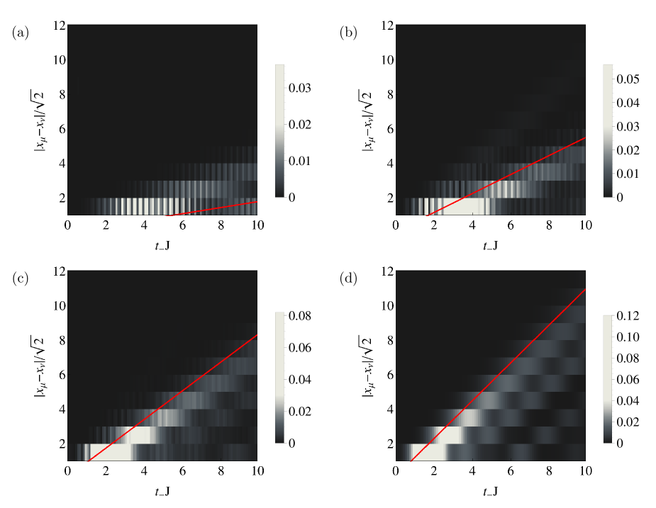
In Fig. 2 we evaluate the double-time correlation function for different values of $\beta U$. The density plots show a temperature-dependent light-cone structure. For low temperatures it is viable to neglect occupation numbers $n>2$. The dynamics of the correlation functions w.r.t. to the time difference $t_{-}=(t-t^{\prime})/2$ at unit filling is determined by the frequencies

$$\Omega_{\mathbf{k}}= U-J(1-3p_{0})T_{\mathbf{k}}$$

$$-\sqrt{U^{2}-6J(1-3p_{0})UT_{\mathbf{k}}+J^{2}(1-3p_{0})^{2}T_{\mathbf{k}}^{2}}$$ (22)

with $p_{0}=p_{2}=1/(2+e^{\beta U/2})$ being the probability to find zero or two particles on a lattice site. The maximum group velocity, given by $v^{\mathrm{max}}=\mathrm{max}_{\mathbf{k}}|\nabla_{\mathbf{k}}\Omega_{\mathbf{k}}|$, determines the light-cone structure of the correlations. At zero temperature, the propagation velocity of the correlations is maximal, see Fig. 2 (d). In this limit, only the doublon-holon excitations $\langle P^{10}_{\mu}(t)P^{12}_{\nu}(t^{\prime})\rangle$, $\langle P^{21}_{\mu}(t)P^{01}_{\nu}(t^{\prime})\rangle$, $\langle P^{10}_{\mu}(t)P^{01}_{\nu}(t^{\prime})\rangle$, and $\langle P^{21}_{\mu}(t)P^{12}_{\nu}(t^{\prime})\rangle$ are relevant.

For finite temperatures, we have $1-3p_{0}<1$. According to equation (III), this implies a shrinking propagation velocity, see Fig. 2 (c). If the temperature is increased even further, the approximation of thermal particle-hole excitations is not valid anymore since also occupation numbers $n>2$ play a role. Therefore, the analytical result (III) does not determine the light-cone structure anymore, see Fig. 2 (a) and (b).

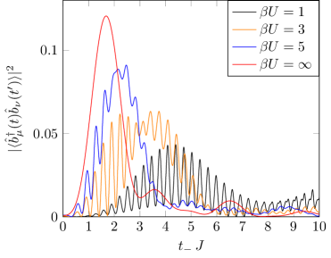
The population of higher excited states is also reflected in the time-evolution of the correlations at a fixed distance $|x_{\mu}-x_{\nu}|$. At $\beta U=\infty$, only eigen-modes of order $\mathcal{O}(U)$ play a role whereas for large temperatures the eigen-modes of order $\mathcal{O}(nU)$, $n>1$ dominate the time-evolution, see Fig. 1.

Figure 1: Double-time correlation for $|x_{\mu}-x_{\nu}|=\sqrt{2}$ in two dimensions at different temperatures. The position of the maximum is shifting with temperature approximately as $(t_{-}J)\sim 1/(1-3p_{0})$.

Figure 2: Time-dependence of the two-time correlation functions $|\langle\hat{b}^{\dagger}(t)\hat{b}(t^{\prime})\rangle_{\mathrm{therm}}|^{2}$ along the diagonal for a lattice in two dimensions for unit filling and $J/U=0.1$. The parameters are (a) $\beta U=1$, (b) $\beta U=3$, (c) $\beta U=5$, (d) $\beta U=\infty$. The maximum velocity of the correlations decreases with the temperature of the thermal ensemble. When the temperature grows, also highly energetic modes contribute to the dynamics. The amplitude of the correlations decreases with increasing temperature.

IV Equilibration after a quantum quench

In this section we turn to the non-equilibrium dynamics of excitations in the Bose-Hubbard system after a quantum quench at finite temperatures from $J=0$ to $J>0$. The evolution of time-local quantities can be deduced from double-time hierarchy for $t=t^{\prime}$ of from the single-time hierarchy in NS10 . Afterwards we compare the pre-thermalized expectation values at $t\rightarrow\infty$ with the corresponding thermal expectation values.

We assume the system to be initially in a thermal state which is determined by the density matrix

$$\hat{\rho}^{\mathrm{in}}=\bigotimes_{\mu}\hat{\rho}_{\mu},\quad\hat{\rho}_{\mu}=\sum_{n}p_{n}|n\rangle_{\mu}\langle n|\,,$$ (23)

where the $p_{n}$ are given by the thermal distribution (18). The hopping rate is switched suddenly from $J=0$ to a finite value which is still in the Mott regime $J<J_{\mathrm{crit}}$. The dynamics of the on-site probabilities follow the equations

$$i\partial_{t}\langle\hat{P}^{n,n}_{\mu}\rangle=-\frac{J}{Z}\sum_{\kappa}T_{\mu\kappa}\sum_{m}\sqrt{m+1}$$ (24)

$$\times \bigg{[}\sqrt{n}\big{(}\langle\hat{P}_{\mu}^{n,n-1}\hat{P}_{\kappa}^{m,m+1}\rangle^{\mathrm{corr}}-\langle\hat{P}_{\kappa}^{m+1,m}\hat{P}_{\mu}^{n-1,n}\rangle^{\mathrm{corr}}\big{)}$$

$$-\sqrt{n+1}\big{(}\langle\hat{P}_{\mu}^{n+1,n}\hat{P}_{\kappa}^{m,m+1}\rangle^{\mathrm{corr}}-\langle\hat{P}_{\kappa}^{m+1,m}\hat{P}_{\mu}^{n,n+1}\rangle^{\mathrm{corr}}\big{)}\bigg{]}\,,$$

and the two-point correlations evolve according to

$$[i\partial_{t}+U(n-m)]\langle\hat{P}^{n+1,n}_{\mu}\hat{P}^{m,m+1}_{\nu}\rangle^{\mathrm{corr}}$$

$$=- \frac{J}{Z}\sqrt{n+1}(\langle\hat{P}^{n+1,n+1}_{\mu}\rangle-\langle\hat{P}^{n,n}_{\mu}\rangle)$$

$$\times\sum_{\kappa\neq\mu,\nu}T_{\kappa\mu}\langle\hat{b}^{\dagger}_{\kappa}\hat{P}^{m,m+1}_{\nu}\rangle^{\mathrm{corr}}$$

$$- \frac{J}{Z}\sqrt{m+1}(\langle\hat{P}^{m,m}_{\nu}\rangle-\langle\hat{P}^{m+1,m+1}_{\nu}\rangle)$$

$$\times\sum_{\kappa\neq\mu,\nu}T_{\kappa\nu}\langle\hat{P}^{n+1,n}_{\mu}\hat{b}_{\kappa}\rangle^{\mathrm{corr}}$$

$$- \frac{J}{Z}T_{\mu\nu}\sqrt{n+1}\sqrt{m+1}\langle\hat{P}^{n+1,n+1}_{\mu}\rangle\langle\hat{P}^{m,m}_{\nu}\rangle$$

$$+ \frac{J}{Z}T_{\mu\nu}\sqrt{n+1}\sqrt{m+1}\langle\hat{P}^{n,n}_{\mu}\rangle\langle\hat{P}^{m+1,m+1}_{\nu}\rangle\,.$$ (25)

In the limit of zero temperature, the doublon-holon correlation functions decouple from correlation functions which involve occupation numbers $n>2$. This case has been discussed in references NS10 ; QKNS14 . However, we shall see that a finite temperature alters the pre-thermalization dynamics.

The equations (24) and (IV) are nonlinear due to the back-reaction of the on-site quantities onto the correlations. This back-reaction can be neglected since it is of order $1/Z^{2}$ and we have $\langle\hat{P}^{n,n}_{\mu}\rangle=P_{n}=p_{n}+\mathcal{O}(1/Z)$. Exploiting the translational symmetry, we can simplify these equations by a spatial Fourier transformation

$$\langle\hat{P}_{\mu}^{n,n-1}\hat{P}_{\nu}^{m-1,m}\rangle=\frac{1}{N}\sum_{\mathbf{k}}f^{n,m}_{\mathbf{k}}e^{i\mathbf{k}\cdot(\mathbf{x}_{\mu}-\mathbf{x}_{\nu})}\,,$$ (26)

where $N$ denotes the number of lattice sites. Now, the on-site probabilities $P_{n}=\langle\hat{P}^{n,n}_{\mu}\rangle$ evolve according to

$$i\partial_{t}P_{n}= -\frac{J}{N}\sum_{\mathbf{k}}T_{\mathbf{k}}\sum_{m}\sqrt{m+1}$$

$$\times\bigg{[}\sqrt{n}\big{(}f_{\mathbf{k}}^{n,m+1}-f_{\mathbf{k}}^{m+1,n}\big{)}$$

$$-\sqrt{n+1}\big{(}f_{\mathbf{k}}^{n+1,m+1}-f_{\mathbf{k}}^{m+1,n+1}\big{)}\bigg{]}\,,$$ (27)

whereas for the Fourier components of the correlations we find

$$[i\partial_{t}+U(n-m)]f_{\mathbf{k}}^{n+1,m+1}$$

$$=-JT_{\mathbf{k}}\sqrt{n+1}(p_{n+1}-p_{n})\sum_{s=0}^{\infty}\sqrt{s+1}f_{\mathbf{k}}^{s+1,m+1}$$

$$-JT_{\mathbf{k}}\sqrt{m+1}(p_{m}-p_{m+1})\sum_{s=0}^{\infty}\sqrt{s+1}f_{\mathbf{k}}^{n+1,s+1}$$

$$-JT_{\mathbf{k}}\sqrt{m+1}\sqrt{n+1}(p_{n+1}p_{m}-p_{n}p_{m+1})\,.$$ (28)

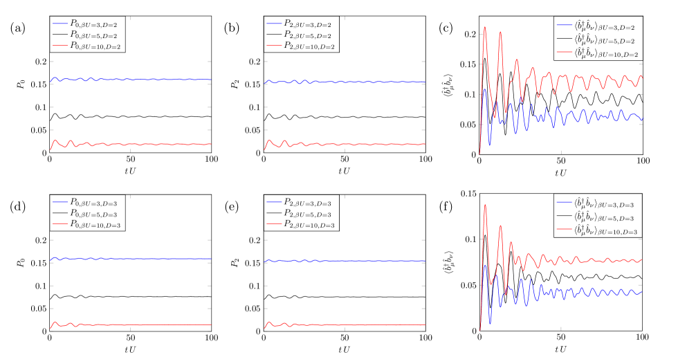
We solved the coupled system of equations in two and three dimensions for various temperatures, see Fig. 4. The on-site probabilities are oscillating around their initial thermal value $p_{n}$. Especially for high temperatures, the back action of these quantities onto the correlation functions can indeed be safely neglected since$|P_{n}(t)-P_{n}(0)|/P_{n}(0)\ll 1$.

In order to gain some analytical insight into the equilibration process, we neglect $p_{n}$ for $n>2$. As a consequence, we obtain the particle-hole symmetry $p_{0}=p_{2}$. When the system is quenched from a thermal state, the oscillations decrease with time and the on-site probabilities approach for $t\rightarrow\infty$

$$P_{0/2,\mathrm{equil}}=p_{0}+\frac{1}{N}\sum_{\mathbf{k}}\frac{4J^{2}T_{\mathbf{k}}^{2}(1-4p_{0}+3p_{0}^{2})}{\omega_{\mathbf{k}}^{2}}$$ (29)

with

$$\omega_{\mathbf{k}}= \sqrt{\big{[}U^{2}-6JT_{\mathbf{k}}(1-3p_{0})U+J^{2}T_{\mathbf{k}}^{2}(1-3p_{0})^{2}\big{]}}\,.$$ (30)

For the lattice-site correlations we for $t\rightarrow\infty$ the asymptotic expression

$$\langle\hat{b}^{\dagger}_{\mu}\hat{b}_{\nu}\rangle_{\mathrm{equil}}=\frac{1}{N}\sum_{\mathbf{k}}e^{i\mathbf{k}\cdot(\mathbf{x}_{\mu}-\mathbf{x}_{\nu})}\frac{4JT_{\mathbf{k}}U(1-4p_{0}+3p_{0}^{2})}{\omega_{\mathbf{k}}^{2}}\,.$$ (31)

Given equations (29) and (31), we conclude that the quench-induced change of these quantities becomes smaller with increasing temperature.

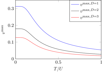
From the eigen-modes we can also estimate the maximum propagation speed of the expanding correlations. As before, we can estimate the maximum propagation velocity from $v^{\mathrm{max}}=\mathrm{max}_{\mathbf{k}}|\nabla_{\mathbf{k}}\Omega_{\mathbf{k}}|$. In a hyper-cubic lattice in $D$ dimensions with small $J/U$ we have $v^{\mathrm{max}}=J(3-9p_{0})/D$ along the lattice axes and $v^{\mathrm{max}}=J(3-9p_{0})/\sqrt{D}$ along the diagonals. As before, the maximum propagation speed becomes smaller for increasing temperatures, see Fig. 3.

Figure 3: The maximum velocity of the correlations after a quantum quench from $J=0$ to $J/U=0.1$ depends on the temperature of the initial ensemble.

Figure 4: Equilibration dynamics in two and three dimensions. The amplitude of the oscillations decreases with increasing temperature of the initial state. For all initial temperatues, the system prethermalizes faster in three dimensions than it does in two dimensions. In our computation, we did not restrict the occupation number. Nevertheless, we see that also for finite but sufficiently low temperatures, the particle-hole symmetry is approximately valid.

The pre-thermalized state is a quasi-stationary state which is not necessarily thermal whereas real thermalization occurs on much longer time-scales BBS03 ; BBW04 ; KWE11 . However, we can compare the pre-thermalized state with a corresponding thermal state that has the same temperature $T$ and filling $\langle\hat{n}_{\mu}\rangle$. In order to do so, we compute the asymptotic values of the on-site probabilities $P_{n,\mathrm{equil}}$ and the correlation functions $\langle\hat{b}_{\mu}^{\dagger}\hat{b}_{\nu}\rangle_{\mathrm{equil}}$ from equations (IV) and (IV) without further approximations. The thermal correlation $\langle\hat{b}_{\mu}^{\dagger}\hat{b}_{\nu}\rangle_{\mathrm{therm}}$ can be deduced from equation (III). For the order $\mathcal{O}(1/Z)$-contribution of the $P_{n,\mathrm{therm}}$ we take the expression from reference NQS16 . In this article, we evaluated the partition function of the Bose-Hubbard system up to $\mathcal{O}(1/Z)$ and derived various thermal quantities. Explicitly we have (see equation 21 in NQS16 )

$$P_{n,\mathrm{therm}}= p_{n}+\frac{1}{N}\sum_{\mathbf{k}}\sum_{l=-\infty}^{\infty}\frac{JT_{\mathbf{k}}}{1+JT_{\mathbf{k}}G(\omega_{l})}\bigg{[}p_{n}G(\omega_{l})$$

$$-\frac{(n+1)p_{n}}{\omega_{l}-Un+\mu}+\frac{np_{n}}{\omega_{l}-U(n-1)+\mu}$$

$$+\frac{n(p_{n-1}-p_{n})}{\beta(\omega_{l}-U(n-1)+\mu)^{2})^{2}}$$

$$-\frac{(n+1)(p_{n}-p_{n+1})}{\beta(\omega_{l}-Un+\mu)^{2}}\bigg{]}$$ (32)

with the bosonic Matsubara modes $\omega_{l}=2\pi il/\beta$.

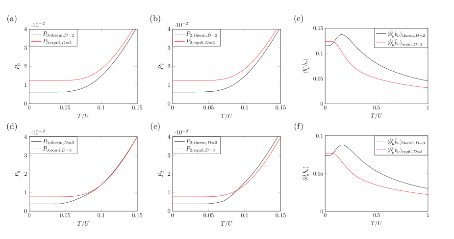
At zero temperature, the values differ roughly by a factor of 2 which has been stated elsewhere MK09 . For sufficiently low temperatures, the particle-hole symmetry is valid, $P_{0}\sim P_{2}$, which can be deduced from comparing Fig. 5 (a) and (b) or Fig. 5 (d) and (e). The energy which is transferred by a quench to the system becomes more and more irrelevant for increasing temperatures. Thus, the difference between thermal and pre-thermalized quantities reduces with growing $T$. From Fig. 5 (c) and (f) we see how the increasing temperature diminishes the correlations between lattice sites. However, the thermal next neighbor correlation function has its global maximum at finite $T>0$.

Figure 5: After a quantum quench at a temperature $T$, the occupation probabilities and the correlation functions approach a prethermalized value (red curves). This is compared with the corresponding thermal expressions (black curves). For low temperatures, the onsite-quantities differ roughly by a factor of 2. The difference between prethermalized and thermal values diminishes with increasing temperatures. Note that deviations from the particle-hole symmetry at high temperatures are larger in three dimensions (see (d) and (e)) than in two dimensions (see (d) and (e)). In (c) and (f) we depict the temperature-dependence of the prethermalized and thermal expectation values of the next neighbour correlations $\langle\hat{b}_{\mu}^{\dagger}\hat{b}_{\nu}\rangle$. Note that the thermal correlation function has its global maximum at $T>0$.

V Quantum quench and Double-time correlations

A quantum quench changes also the light-cone structure of the double-time correlation functions. We assume that before the quantum quench the system is in an equilibrium state with a finite hopping rate $J_{-}$. At time $t=0$, the hopping rate is quenched to a value $J_{+}<J_{\mathrm{crit}}$. For simplicity, we restrict our considerations to zero temperature. Analogous to equation (26) we define the Fourier transform of the two-time correlations

$$\langle\hat{P}_{\mu}^{n,n-1}(t)\hat{P}_{\nu}^{m-1,m}(t^{\prime})\rangle=\frac{1}{N}\sum_{\mathbf{k}}f^{n,m}_{\mathbf{k}}(t,t^{\prime})e^{i\mathbf{k}\cdot(\mathbf{x}_{\mu}-\mathbf{x}_{\nu})}\,.$$ (33)

The dynamics of the correlation functions follows directly from equation (II) and a corresponding relation which takes into account the time-evolution w.r.t. variable $t^{\prime}$. Neglecting the back-reaction onto the on-site probabilities, the Fourier coefficients evolve up to order $1/Z$ according to

$$i\partial_{t}f^{11}_{\mathbf{k}} =-J^{\pm}T_{\mathbf{k}}(f_{\mathbf{k}}^{11}+\sqrt{2}f_{\mathbf{k}}^{21})-J^{\pm}T_{\mathbf{k}}\,,$$ (34)

$$i\partial_{t}f^{12}_{\mathbf{k}} =-J^{\pm}T_{\mathbf{k}}(f_{\mathbf{k}}^{12}+\sqrt{2}f_{\mathbf{k}}^{22})\,,$$ (35)

$$i\partial_{t}f^{21}_{\mathbf{k}} =\sqrt{2}J^{\pm}T_{\mathbf{k}}(f_{\mathbf{k}}^{11}+\sqrt{2}f_{\mathbf{k}}^{21})-Uf_{\mathbf{k}}^{21}+\sqrt{2}J^{\pm}T_{\mathbf{k}}\,,$$ (36)

$$i\partial_{t}f^{22}_{\mathbf{k}} =\sqrt{2}J^{\pm}T_{\mathbf{k}}(f_{\mathbf{k}}^{12}+\sqrt{2}f_{\mathbf{k}}^{22})-Uf_{\mathbf{k}}^{22}\,,$$ (37)

and

$$i\partial_{t^{\prime}}f^{11}_{\mathbf{k}} =J^{\pm}T_{\mathbf{k}}(f_{\mathbf{k}}^{11}+\sqrt{2}f_{\mathbf{k}}^{12})+J^{\pm}T_{\mathbf{k}}\,,$$ (38)

$$i\partial_{t^{\prime}}f^{12}_{\mathbf{k}} =-\sqrt{2}J^{\pm}T_{\mathbf{k}}(f_{\mathbf{k}}^{11}+\sqrt{2}f_{\mathbf{k}}^{12})+Uf_{\mathbf{k}}^{12}-\sqrt{2}J^{\pm}T_{\mathbf{k}}\,,$$ (39)

$$i\partial_{t^{\prime}}f^{21}_{\mathbf{k}} =J^{\pm}T_{\mathbf{k}}(f_{\mathbf{k}}^{21}+\sqrt{2}f_{\mathbf{k}}^{22})\,,$$ (40)

$$i\partial_{t^{\prime}}f^{22}_{\mathbf{k}} =-\sqrt{2}J^{\pm}T_{\mathbf{k}}(f_{\mathbf{k}}^{21}+\sqrt{2}f_{\mathbf{k}}^{22})+Uf_{\mathbf{k}}^{22}\,.$$ (41)

For $t,t^{\prime}<0$, the correlation functions can be immediately obtained from the ground state correlations at $J=J_{-}$ QKNS14 . Due to the quantum quench, the correlation function is not anymore homogeneous in time but depends on the relative time $t_{-}=(t-t^{\prime})/2$ and on the central time $t_{+}=(t+t^{\prime})/2$. For $t_{+}\pm t_{-}<0$ and $t_{+}\pm t_{-}>0$ we find correlations before and after the hopping quench, respectively. Correlations between an creation (annihilation) of a particle before the quench and an annihilation (creation) of particle can be obtained for $t_{+}+t_{-}<0$ and $t_{+}-t_{-}>0$ ($t_{+}+t_{-}>0$ and $t_{+}-t_{-}<0$).

The light-cone structure is primarily determined by three different velocities. For $t,t^{\prime}<0$, the maximum velocity $v^{\mathrm{max}}_{--}=\mathrm{max}_{\mathbf{k}}|\nabla_{\mathbf{k}}\Omega^{--}_{\mathbf{k}}|$ can be estimated from

$$\Omega_{\mathbf{k}}^{--}=U-J_{-}T_{\mathbf{k}}-\sqrt{U^{2}-6J_{-}UT_{\mathbf{k}}+(J_{-}T_{\mathbf{k}})^{2}}\,.$$ (42)

For $t>0$ and $t^{\prime}<0$ or $t<0$ and $t^{\prime}>0$, the spread is determined by both hopping rates $J_{-}$ and $J_{+}$. Thus we have the eigen-modes

$$\Omega_{\mathbf{k}}^{+-}= \frac{1}{2}\left(U-J_{-}T_{\mathbf{k}}-\sqrt{U^{2}-6J_{-}UT_{\mathbf{k}}+(J_{-}T_{\mathbf{k}})^{2}}\right)$$

$$+ \frac{1}{2}\left(U-J_{+}T_{\mathbf{k}}-\sqrt{U^{2}-6J_{+}UT_{\mathbf{k}}+(J_{+}T_{\mathbf{k}})^{2}}\right)\,.$$ (43)

from which one can obtain $v^{\mathrm{max}}_{+-}=\mathrm{max}_{\mathbf{k}}|\nabla_{\mathbf{k}}\Omega^{+-}_{\mathbf{k}}|$. Finally, if $t,t^{\prime}>0$, the spread of correlations is dominantly determined by $J_{+}$. Here the maximum velocity $v^{\mathrm{max}}_{++}=\mathrm{max}_{\mathbf{k}}|\nabla_{\mathbf{k}}\Omega^{++}_{\mathbf{k}}|$ can be derived from

$$\Omega_{\mathbf{k}}^{++}=U-J_{+}T_{\mathbf{k}}-\sqrt{U^{2}-6J_{+}UT_{\mathbf{k}}+(J_{+}T_{\mathbf{k}})^{2}}\,.$$ (44)

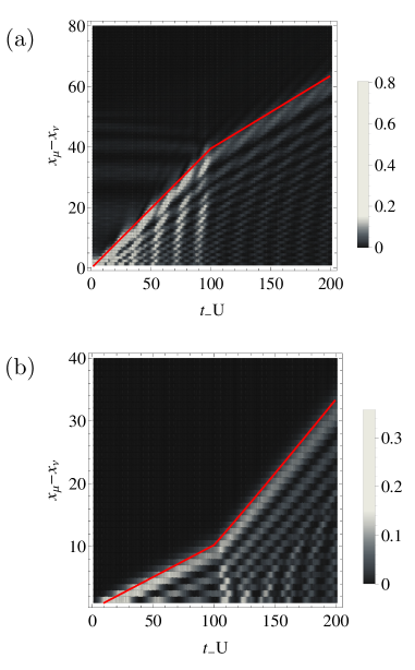
The kink in the light-cone structure due to the quantum quench is illustrated in Fig. 6. The complete light-cone structure for the double-time correlators in arbitrary dimensions is evaluated in appendix VIII.

Figure 6: Double-time correlation function $\langle\hat{b}^{\dagger}_{\mu}(t)\hat{b}_{\nu}(t^{\prime})\rangle_{T=0}$ in one dimension for a quench at $t=0$ from $J_{-}/U=0.05$ to $J_{+}/U=0.15$. (a): $t_{+}U=100$, the lightcone has a kink at $t_{-}=t_{+}$ where the maximum velocity changes from $v^{\mathrm{max}}_{++}\approx 0.40$ to $v^{\mathrm{max}}_{+-}\approx 0.24$. (b): $t_{+}U=-100$, the lightcone has a kink at $t_{-}=-t_{+}$ where the maximum velocity changes from $v^{\mathrm{max}}_{--}\approx 0.10$ to $v^{\mathrm{max}}_{+-}\approx 0.24$.

VI Conclusions

We studied equilibrium properties and non-equilibrium dynamics of the Bose-Hubbard model in the Mott insulating phase. To this end, we extended the hierarchy for large coordination numbers $Z$ presented in NS10 to a hierarchy for double-time correlation functions.

This enabled us to derive thermal correlation functions and we studied the spread of two-time correlation functions at finite initial temperatures, see Figs. 2 and 1. We restricted our considerations to first order in $1/Z$ which governs the free quasi-particle evolution. As usual, the effective light-cone structure was obtained via a saddle-point approximation.

As we demonstrated above, the dynamics of strongly interacting quantum many-body systems and their thermal properties can be both accessed within our approach. The phenomenon of pre-thermalization after a quantum quench was generalized from $T=0$ QKNS14 to finite temperatures, see Figs. 4 and 3. Note that the dynamical equations in order $\mathcal{O}(1/Z)$ cover only the short-time evolution of the excitations. In order to include the long-time evolution which is determined by quasi-particle scattering, also higher order correlations have to be taken into account. For real thermalization processes, for example, one has to evaluate the hierarichal equations up to order $\mathcal{O}(1/Z^{3})$ in order to obtain a Boltzmann equation QS19a .

Apart from these theoretical investigations, our approach can also be applied in order to interpret experimental results. Since the double-time hierarchy induces a Green function hierarchy, the latter can used for the interpretation of pump-probe experiments . An excitation which is created by a pump beam at time $t$ and measured by a probe beam at time $t^{\prime}$ is naturally described in terms of the lesser Green functions ATE14 ; FMSSD17 ; FKP17 . Moreover, the Green function hierarchy allows for a controlled perturbative calculation of the self-energy or the susceptibility of strongly correlated systems.

As an outlook, the study of out-of-time-correlators (OTOC), a common measure for quantum chaos, should be feasible within our approach LO69 ; MSS16 . In this context one has to extend the double-time hierarchy of correlations to a hierarchy of multi-time correlations. This should be possible in complete analogy to the approach presented in this work and will be the subject of further studies.

VII Appendix: Proof of the hierarchy

The most general double-time expectation value has the form $\langle\hat{A}_{\mathcal{S}}(t)\hat{B}_{\mathcal{S}}(t^{\prime})\rangle$ where $\mathcal{S}$ denotes the set of $|\mathcal{S}|$ lattice sites. In order to avoid cluttering of indices, we introduce a short hand notation for operators which are defined on the set $\mathcal{S}$ via $\hat{A}_{\mathcal{S}}(t)=\hat{A}^{1}_{\mu_{1}}(t)\times...\times A^{n}_{\mu_{n}}(t)$ and $\hat{B}_{\mathcal{S}}(t^{\prime})=\hat{B}^{1}_{\mu_{1}}(t^{\prime})\times...\times\hat{B}^{n}_{\mu_{n}}(t^{\prime})$. From the equation-of-motion hierarchy for the expectation values $\langle\hat{A}_{\mathcal{S}}(t)\hat{B}_{\mathcal{S}}(t^{\prime})\rangle$, the hierarchy for expectation values of the form $\langle\hat{A}(t)_{\mathcal{P}_{1}}\hat{B}_{\mathcal{P}_{2}}(t^{\prime})\rangle$ can be obtained by setting $\mathcal{S}=\mathcal{P}_{1}\cup\mathcal{P}_{2}$ and choosing $\hat{A}_{\mu}(t)=\hat{1}_{\mu}$ for $\mu\notin\mathcal{P}_{1}$ and $\hat{B}_{\nu}(t^{\prime})=\hat{1}_{\nu}$ for $\nu\notin\mathcal{P}_{2}$.

In NS10 , we presented a hierarchy for the correlated parts of a many-particle density matrix based on a large coordination number $Z$. This hierarchy was formulated for operators but it can also be stated in terms of correlation functions. In the following, we will derive the corresponding hierarchy for two-time correlation functions . The starting point is a separation of the correlation functions in correlated and uncorrelated parts. For two sites, the correlated part of an expectation values is defined by as

$$\langle\hat{A}_{\mu}(t)\hat{B}_{\nu}(t)\hat{C}_{\mu}(t^{\prime})\hat{D}_{\nu}(t^{\prime})\rangle^{\mathrm{c}}=\langle\hat{A}_{\mu}(t)\hat{B}_{\nu}(t)\hat{C}_{\mu}(t^{\prime})\hat{D}_{\nu}(t^{\prime})\rangle-\langle\hat{A}_{\mu}(t)\hat{C}_{\mu}(t^{\prime})\rangle\langle\hat{B}_{\nu}(t)\hat{D}_{\nu}(t^{\prime})\rangle\,.$$ (45)

Arbitrary correlation functions can be separated according to

$$\langle\hat{A}_{\cal S}(t)\hat{B}_{\cal S}(t^{\prime})\rangle^{\mathrm{c}} =\langle\hat{A}_{\cal S}(t)\hat{B}_{\cal S}(t^{\prime})\rangle-\sum_{\cup_{i}{\cal{P}}_{i}={\cal{S}},{{\cal P}}_{i}\subset{\cal{S}}}\prod_{{\cal P}_{i}}\langle\hat{A}_{{\cal{P}}_{i}}(t)\hat{B}_{{\cal{P}}_{i}}(t^{\prime})\rangle^{\mathrm{c}}\,,$$ (46)

where the sum is over all proper partitions of the set $\cal{S}$. Note that the definition of the correlated parts agrees with the separation of the density matrix into correlated parts given in NS10 if the operators depending on $t$ (or $t^{\prime}$) are replaced by the unity operator. The central point of our derivation is the scaling hierarchy of the correlations,

$$\langle\hat{A}_{\mathcal{S}}(t)\hat{B}_{\mathcal{S}}(t^{\prime})\rangle^{\mathrm{c}}=\mathcal{O}(Z^{1-|\mathcal{S}|})\,.$$ (47)

Rewriting the hierarchy of the density matrix from reference NS10 in terms of expectation values it is possible to guess the corresponding hierarchy for for the equations of motion of $\langle\hat{A}_{\mathcal{S}}(t)\hat{B}_{\mathcal{S}}(t^{\prime})\rangle^{\mathrm{c}}$. We claim that the full hierarchy for an arbitrary set of $\mathcal{S}$ lattice sites has the form

$$i\partial_{t}\langle\hat{A}_{\cal S}(t)\hat{B}_{\cal S}(t^{\prime})\rangle^{\mathrm{c}} =\sum_{\mu\in{\cal S}}\langle[\hat{A}_{\mathcal{S}}(t),\hat{H}_{\mu}(t)]\hat{B}_{\cal S}(t^{\prime})\rangle^{\mathrm{c}}-\frac{J}{Z}\sum_{\mu,\nu\in\mathcal{S}}T_{\mu\nu}\langle[\hat{A}_{\mathcal{S}}(t),\hat{X}_{\mu}^{\dagger}(t)\hat{X}_{\nu}(t)]\hat{B}_{\cal S}(t^{\prime})\rangle^{\mathrm{c}}$$ (48a)

$$-\frac{J}{Z}\sum_{\kappa\notin\mathcal{S}}\sum_{\mu\in S}T_{\mu\kappa}\bigg{\{}\langle\hat{X}^{\dagger}_{\kappa}(t)[\hat{A}_{\mathcal{S}}(t),\hat{X}_{\mu}(t)]\hat{B}_{\mathcal{S}}(t^{\prime})\rangle^{\mathrm{c}}+\langle\hat{X}_{\kappa}(t)[\hat{A}_{\mathcal{S}}(t),\hat{X}_{\mu}^{\dagger}(t)]\hat{B}_{\mathcal{S}}(t^{\prime})\rangle^{\mathrm{c}}\bigg{\}}$$ (48b)

$$-\frac{J}{Z}\sum_{\kappa\notin\mathcal{S}}\sum_{\mu\in\mathcal{S}}\sum_{\mathcal{P}\subseteq\mathcal{S}\setminus\{\mu\}}^{\mathcal{P}\cup\bar{\mathcal{P}}=\mathcal{S}\setminus\{\mu\}}T_{\mu\kappa}\bigg{\{}\langle[\hat{A}_{\mathcal{P}\cup\{\mu\}}(t),\hat{X}_{\mu}(t)]\hat{B}_{\mathcal{P}\cup\{\mu\}}(t^{\prime})\rangle^{\mathrm{c}}\langle\hat{X}^{\dagger}_{\kappa}(t)\hat{A}_{\bar{\mathcal{P}}}(t)\hat{B}_{\bar{\mathcal{P}}}(t^{\prime})\rangle^{\mathrm{c}}$$ (48c)

$$\hskip 42.67912pt+\langle[\hat{A}_{\mathcal{P}\cup\{\mu\}}(t),\hat{X}_{\mu}^{\dagger}(t)]\hat{B}_{\mathcal{P}\cup\{\mu\}}(t^{\prime})\rangle^{\mathrm{c}}\langle\hat{X}_{\kappa}(t)\hat{A}_{\bar{\mathcal{P}}}(t)\hat{B}_{\bar{\mathcal{P}}}(t^{\prime})\rangle^{\mathrm{c}}\bigg{\}}$$ (48d)

$$-\frac{J}{Z}\sum_{\mu,\nu\in\mathcal{S}}\sum_{\mathcal{P}\subseteq\mathcal{S}\setminus\{\mu,\nu\}}^{\mathcal{P}\cup\bar{\mathcal{P}}=\mathcal{S}\setminus\{\mu,\nu\}}T_{\mu\nu}\Bigg{\{}\langle[\hat{A}_{\mathcal{P}\cup\{\mu\}}(t),\hat{X}^{\dagger}_{\mu}(t)]\hat{B}_{\mathcal{P}\cup\{\mu\}}(t^{\prime})\rangle^{\mathrm{c}}\langle\hat{X}_{\nu}(t)\hat{A}_{\bar{\mathcal{P}}\cup\{\nu\}}(t)\hat{B}_{\bar{\mathcal{P}}\cup\{\nu\}}(t^{\prime})\rangle^{\mathrm{c}}$$ (48e)

$$\hskip 42.67912pt+\langle\hat{A}_{\mathcal{P}\cup\{\mu\}}(t)\hat{X}_{\mu}^{\dagger}(t)\hat{B}_{\mathcal{P}\cup\{\mu\}}(t^{\prime})\rangle^{\mathrm{c}}\langle[\hat{A}_{\bar{\mathcal{P}}\cup\{\nu\}}(t),\hat{X}_{\nu}(t)]\hat{B}_{\bar{\mathcal{P}}\cup\{\nu\}}(t^{\prime})\rangle^{\mathrm{c}}$$ (48f)

$$-\langle\hat{A}_{\mathcal{P}\cup\nu}(t)\hat{B}_{\mathcal{P}\cup\nu}(t^{\prime})\rangle^{\mathrm{c}}\Bigg{[}\langle\hat{X}^{\dagger}_{\nu}(t)[\hat{A}_{\bar{\mathcal{P}}\cup\{\mu\}}(t),\hat{X}_{\mu}(t)]\hat{B}_{\bar{\mathcal{P}}\cup\{\mu\}}(t^{\prime})\rangle^{\mathrm{c}}+\langle\hat{X}_{\nu}(t)[\hat{A}_{\bar{\mathcal{P}}\cup\{\mu\}}(t),\hat{X}^{\dagger}_{\mu}(t)]\hat{B}_{\bar{\mathcal{P}}\cup\{\mu\}}(t^{\prime})\rangle^{\mathrm{c}}$$ (48g)

$$+\sum_{\mathcal{Q}\subseteq\bar{\mathcal{P}}}^{\mathcal{Q}\cup\bar{\mathcal{Q}}=\bar{\mathcal{P}}}\bigg{(}\langle[\hat{A}_{\mathcal{Q}\cup\{\mu\}}(t),\hat{X}_{\mu}(t)]\hat{B}_{\mathcal{Q}\cup\{\mu\}}(t^{\prime})\rangle^{\mathrm{c}}\langle\hat{X}^{\dagger}_{\nu}(t)\hat{A}_{\bar{\mathcal{Q}}}(t)\hat{B}_{\bar{\mathcal{Q}}}(t^{\prime})\rangle^{\mathrm{c}}$$ (48h)

$$\hskip 42.67912pt+\langle[\hat{A}_{\mathcal{Q}\cup\{\mu\}}(t),\hat{X}_{\mu}^{\dagger}(t)]\hat{B}_{\mathcal{Q}\cup\{\mu\}}(t^{\prime})\rangle^{\mathrm{c}}\langle\hat{X}_{\nu}(t)\hat{A}_{\bar{\mathcal{Q}}}(t)\hat{B}_{\bar{\mathcal{Q}}}(t^{\prime})\rangle^{\mathrm{c}}\bigg{)}\Bigg{]}\Bigg{\}}$$ (48i)

We will restrict ourselves to bosonic systems for proving (48a)-(48i) by induction. For fermionic operators, additional signs will appear due to the permutations of the operators $\hat{A}_{\mu}$ and $\hat{B}_{\mu}$ in the partitions of the expectation values in correlated parts.

To begin, we assume that the hierarchy holds for all sets of lattice sites with cardinality strictly less then $|\cal{S}|$. From this we will derive the equations of motion for a set with cardinality equal to $|\cal{S}|$. The Heisenberg equations of motion for the operator $\hat{A}_{\cal{S}}$ lead to

$$i\partial_{t}\langle\hat{A}_{\cal{S}}(t)\hat{B}_{\cal{S}}(t^{\prime})\rangle = \sum_{\mu\in{\cal S}}\langle[\hat{A}_{\mathcal{S}}(t),\hat{H}_{\mu}(t)]\hat{B}_{\cal S}(t^{\prime})\rangle-\frac{J}{Z}\sum_{\mu,\nu\in{\cal{S}}}T_{\mu\nu}\langle[\hat{A}_{\cal{S}}(t),\hat{X}_{\mu}^{\dagger}(t)\hat{X}_{\nu}(t)]\hat{B}_{\cal{S}}(t^{\prime})\rangle$$ (49)

$$-\frac{J}{Z}\sum_{\kappa\notin\cal{S}}\sum_{\mu\in\cal{S}}T_{\mu\kappa}\langle\hat{X}_{\kappa}^{\dagger}(t)[\hat{A}_{\cal{S}}(t),\hat{X}_{\mu}(t)]\hat{B}_{\cal{S}}(t^{\prime})\rangle-\frac{J}{Z}\sum_{\kappa\notin\cal{S}}\sum_{\mu\in\cal{S}}T_{\mu\kappa}\langle\hat{X}_{\kappa}(t)[\hat{A}_{\cal{S}}(t),\hat{X}_{\mu}^{\dagger}(t)]\hat{B}_{\cal{S}}(t^{\prime})\rangle$$

As a next step, we separate the expectation values into correlated parts according to (46). The first term can be written as

$$(0)\equiv\sum_{\mu\in{\cal S}}\langle[\hat{A}_{\mathcal{S}}(t),\hat{H}_{\mu}(t)]\hat{B}_{\cal S}(t^{\prime})\rangle=\sum_{{\cal P}\subseteq{\cal S}\setminus\{\mu\}}\langle[\hat{A}_{\mathcal{P}\cup\{\mu\}}(t),\hat{H}_{\mu}(t)]\hat{B}_{\mathcal{P}\cup\{\mu\}}(t^{\prime})\rangle\sum_{\cup_{i}{\cal{P}}_{i}=\cal{S}\setminus\cal{P}\cup\{\mu\}}\prod_{{\cal{P}}_{i}}\langle\hat{A}_{{\cal{P}}_{i}}(t)\hat{B}_{{\cal{P}}_{i}}(t^{\prime})\rangle^{\mathrm{c}}\,.$$ (50)

The second term on the right hand side of equation (49) can be expanded as

$$-\frac{J}{Z}\sum_{\mu,\nu\in{\cal{S}}}T_{\mu\nu}\langle[\hat{A}_{\cal{S}}(t),\hat{X}_{\mu}^{\dagger}(t)\hat{X}_{\nu}(t)]\hat{B}_{\cal{S}}(t^{\prime})\rangle=(1)+(2a)+(2b)$$ (51)

$$= -\frac{J}{Z}\sum_{\mu,\nu\in\cal{S}}T_{\mu\nu}\sum_{{\cal{P}}\subseteq\cal{S}\setminus\{\mu,\nu\}}\Bigg{\{}\langle[\hat{A}_{\cal{P}\cup\{\mu\nu\}}(t),\hat{X}_{\mu}(t)^{\dagger}\hat{X}_{\nu}(t)]\hat{B}_{\cal{P}\cup\{\mu\nu\}}(t^{\prime})\rangle^{\mathrm{c}}$$

$$+\sum_{\cal{Q}\subseteq{\cal{P}}}^{\cal{Q}\cup\bar{\cal{Q}}={\cal{P}}}\Bigg{[}\langle[\hat{A}_{\cal{Q}\cup\{\mu\}}(t),\hat{X}^{\dagger}_{\mu}(t)]\hat{B}_{\cal{Q}\cup\{\mu\}}(t^{\prime})\rangle^{\mathrm{c}}\langle\hat{X}_{\nu}(t)\hat{A}_{\bar{\cal{Q}}(t)\cup\{\nu\}}(t)\hat{B}_{\bar{\cal{Q}}\cup\{\nu\}}(t^{\prime})\rangle^{\mathrm{c}}$$

$$+\langle\hat{A}_{\cal{Q}\cup\{\mu\}}(t)\hat{X}^{\dagger}_{\mu}(t)\hat{B}_{\cal{Q}\cup\{\mu\}}(t^{\prime})\rangle^{\mathrm{c}}\langle[\hat{A}_{\bar{\cal{Q}}\cup\{\nu\}}(t),\hat{X}_{\nu}(t)]\hat{B}_{\bar{\cal{Q}}\cup\{\nu\}}(t^{\prime})\rangle^{\mathrm{c}}\Bigg{]}\Bigg{\}}\sum_{\cup_{i}{\cal{P}}_{i}=\cal{S}\setminus\cal{P}\cup\{\mu,\nu\}}\prod_{{\cal{P}}_{i}}\langle\hat{A}_{{\cal{P}}_{i}}(t)\hat{B}_{{\cal{P}}_{i}}(t^{\prime})\rangle^{\mathrm{c}}$$

For brevety we denoted the three terms in equation (51) with $(1)$, $(2a)$ and $(2b)$. The third term in equation (49) can be written as

$$-\frac{J}{Z}\sum_{\kappa\notin\cal{S}}\sum_{\mu\in\cal{S}}T_{\mu\kappa}\langle\hat{X}_{\kappa}^{\dagger}(t)[\hat{A}_{\cal{S}}(t),\hat{X}_{\mu}(t)]\hat{B}_{\cal{S}}(t^{\prime})\rangle=(3a)+(4a)$$ (52)

$$= -\frac{J}{Z}\sum_{\kappa\notin\cal{S}}\sum_{\mu\in\cal{S}}T_{\mu\kappa}\sum_{\cal{P}\subseteq\cal{S}\setminus\{\mu\}}\Bigg{\{}\langle\hat{X}_{\kappa}^{\dagger}(t)[\hat{A}_{\cal{P}\cup\{\mu\}}(t),\hat{X}_{\mu}(t)]\hat{B}_{\cal{P}\cup\{\mu\}}(t^{\prime})\rangle^{\mathrm{c}}$$

$$+\sum_{\cal{Q}\subseteq\cal{P}}^{\cal{Q}\cup\bar{\cal{Q}}=\cal{P}}\langle[\hat{A}_{\cal{Q}\cup\{\mu\}}(t),\hat{X}_{\mu}(t)]\hat{B}_{\cal{Q}\cup\{\mu\}}(t^{\prime})\rangle^{\mathrm{c}}\langle\hat{X}_{\kappa}^{\dagger}(t)\hat{A}_{\bar{\cal{Q}}}(t)\hat{B}_{\bar{\cal{Q}}}(t^{\prime})\rangle^{\mathrm{c}}\Bigg{\}}\sum_{\cup_{i}{\cal{P}}_{i}=\cal{S}\setminus\cal{P}\cup\{\mu\}}\prod_{{\cal{P}}_{i}}\langle\hat{A}_{{\cal{P}}_{i}}(t)\hat{B}_{{\cal{P}}_{i}}(t^{\prime})\rangle^{\mathrm{c}}$$

Similarly, for the last summand in equation (49) we have

$$-\frac{J}{Z}\sum_{\kappa\notin\cal{S}}\sum_{\mu\in\cal{S}}T_{\mu\kappa}\langle\hat{X}_{\kappa}(t)[\hat{A}_{\cal{S}}(t),\hat{X}^{\dagger}_{\mu}(t)]\hat{B}_{\cal{S}}(t^{\prime})\rangle=(3b)+(4b)$$ (53)

$$= -\frac{J}{Z}\sum_{\kappa\notin\cal{S}}\sum_{\mu\in\cal{S}}T_{\mu\kappa}\sum_{\cal{P}\subseteq\cal{S}\setminus\{\mu\}}\Bigg{\{}\langle\hat{X}_{\kappa}(t)[\hat{A}_{\cal{P}\cup\{\mu\}}(t),\hat{X}^{\dagger}_{\mu}(t)]\hat{B}_{\cal{P}\cup\{\mu\}}(t^{\prime})\rangle^{\mathrm{c}}$$

$$+\sum_{\cal{Q}\subseteq\cal{P}}^{\cal{Q}\cup\bar{\cal{Q}}=\cal{P}}\langle[\hat{A}_{\cal{Q}\cup\{\mu\}}(t),\hat{X}^{\dagger}_{\mu}(t)]\hat{B}_{\cal{Q}\cup\{\mu\}}(t^{\prime})\rangle^{\mathrm{c}}\langle\hat{X}_{\kappa}(t)\hat{A}_{\bar{\cal{Q}}}(t)\hat{B}_{\bar{\cal{Q}}}(t^{\prime})\rangle^{\mathrm{c}}\Bigg{\}}\sum_{\cup_{i}{\cal{P}}_{i}=\cal{S}\setminus\cal{P}\cup\{\mu\}}\prod_{{\cal{P}}_{i}}\langle\hat{A}_{{\cal{P}}_{i}}(t)\hat{B}_{{\cal{P}}_{i}}(t^{\prime})\rangle^{\mathrm{c}}$$

Now we consider the equations of motion for the product of all partitions which contain proper subsets of $\cal{S}$. Applying the product rule of differentiation, we find

$$i\partial_{t}\sum_{\cup_{i}{\cal{P}}_{i}={\cal{S}},{{\cal P}}_{i}\subset{\cal{S}}}\prod_{{\cal P}_{i}}\langle\hat{A}_{{\cal{P}}_{i}}(t)\hat{B}_{{\cal{P}}_{i}}(t^{\prime})\rangle^{\mathrm{c}}=\sum_{{\cal P}\subset{\cal S}}(i\partial_{t}\langle\hat{A}_{{\cal{P}}}(t)\hat{B}_{{\cal{P}}}(t^{\prime})\rangle^{\mathrm{c}})\sum_{\cup_{i}{\cal{P}}_{i}={\cal{S}}\setminus{\cal P}}\prod_{{\cal P}_{i}}\langle\hat{A}_{{\cal{P}}_{i}}(t)\hat{B}_{{\cal{P}}_{i}}(t^{\prime})\rangle^{\mathrm{c}}\,.$$ (54)

The time derivative of $\langle\hat{A}_{{\cal{P}}}(t)\hat{B}_{{\cal{P}}}(t^{\prime})\rangle^{\mathrm{c}}$ can be expressed using (48a)-(48i). Substituting the first term in (48a) to equation (54) leads to

$$(0^{\prime})\equiv\sum_{{\cal P}\subset{\cal S}\setminus\{\mu\}}\langle[\hat{A}_{\mathcal{P}\cup\{\mu\}}(t),\hat{H}_{\mu}(t)]\hat{B}_{\mathcal{P}\cup\{\mu\}}(t^{\prime})\rangle\sum_{\cup_{i}{\cal{P}}_{i}=\cal{S}\setminus\cal{P}\cup\{\mu\}}\prod_{{\cal{P}}_{i}}\langle\hat{A}_{{\cal{P}}_{i}}(t)\hat{B}_{{\cal{P}}_{i}}(t^{\prime})\rangle^{\mathrm{c}}\,,$$ (55)

which is the expression (50) without the summand ${\cal P}={\cal S}\setminus\{\mu\}$. Therefore we find

$$(0)-(0^{\prime})=\sum_{\mu\in{\cal S}}\langle[\hat{A}_{\mathcal{S}}(t),\hat{H}_{\mu}(t)]\hat{B}_{\cal S}(t^{\prime})\rangle^{\mathrm{c}}\,.$$ (56)

The contribution of the second term in (48a) to equation (54) gives

$$(1^{\prime})\equiv-\frac{J}{Z}\sum_{{\cal P}\subset{\cal S}}\sum_{\mu,\nu\in{{\cal P}}}T_{\mu\nu}\langle[\hat{A}_{{\cal P}}(t),\hat{X}_{\mu}^{\dagger}(t)\hat{X}_{\nu}(t)]\hat{B}_{{\cal P}}(t^{\prime})\rangle^{\mathrm{c}}\sum_{\cup_{i}{\cal{P}}_{i}={\cal{S}}\setminus{\cal P}}\prod_{{\cal P}_{i}}\langle\hat{A}_{{\cal{P}}_{i}}(t)\hat{B}_{{\cal{P}}_{i}}(t^{\prime})\rangle^{\mathrm{c}}$$ (57)

In equation (57), the term ${\cal P}={\cal S}$ is excluded from the summation, contrary to equation (51), thus

$$(1)-(1^{\prime})=-\frac{J}{Z}\sum_{\mu,\nu\in\mathcal{S}}T_{\mu\nu}\langle[\hat{A}_{\mathcal{S}}(t),\hat{X}_{\mu}^{\dagger}(t)\hat{X}_{\nu}(t)]\hat{B}_{\cal S}(t^{\prime})\rangle^{\mathrm{c}}\,.$$ (58)

The term (48e) together with (54) leads to

$$(2a^{\prime}) \equiv -\frac{J}{Z}\sum_{{\cal P}\subset{\cal S}}\sum_{\mu,\nu\in{{\cal P}}}\sum_{{\cal Q}\subseteq{\cal P}\setminus\{\mu,\nu\}}^{{\cal Q}\cup\bar{{\cal Q}}={\cal P}\setminus\{\mu,\nu\}}T_{\mu\nu}\langle[\hat{A}_{\cal{Q}\cup\{\mu\}}(t),\hat{X}^{\dagger}_{\mu}(t)]\hat{B}_{\cal{Q}\cup\{\mu\}}(t^{\prime})\rangle^{\mathrm{c}}\langle\hat{X}_{\nu}(t)\hat{A}_{\bar{\cal{Q}}\cup\{\nu\}}(t)\hat{B}_{\bar{\cal{Q}}\cup\{\nu\}}(t^{\prime})\rangle^{\mathrm{c}}$$ (59)

$$\times\sum_{\cup_{i}{\cal{P}}_{i}={\cal{S}}\setminus{\cal P}}\prod_{{\cal P}_{i}}\langle\hat{A}_{{\cal{P}}_{i}}(t)\hat{B}_{{\cal{P}}_{i}}(t^{\prime})\rangle^{\mathrm{c}}$$

Using the same reasoning as above we find the difference

$$(2a)-(2a^{\prime})=-\frac{J}{Z}\sum_{\mu,\nu\in{{\cal S}}}\sum_{{\cal Q}\subseteq{\cal S}\setminus\{\mu,\nu\}}^{{\cal Q}\cup\bar{{\cal Q}}={\cal S}\setminus\{\mu,\nu\}}T_{\mu\nu}\langle[\hat{A}_{\cal{Q}\cup\{\mu\}}(t),\hat{X}^{\dagger}_{\mu}(t)]\hat{B}_{\cal{Q}\cup\{\mu\}}(t^{\prime})\rangle^{\mathrm{c}}\langle\hat{X}_{\nu}(t)\hat{A}_{\bar{\cal{Q}}\cup\{\nu\}}(t)\hat{B}_{\bar{\cal{Q}}\cup\{\nu\}}(t^{\prime})\rangle^{\mathrm{c}}$$ (60)

The part (48f) from the hierarchy together with (54) leads to an expression $(2b^{\prime})$ which has to be substracted from $(2b)$ from equation (51),

$$(2b)-(2b^{\prime})=-\frac{J}{Z}\sum_{\mu,\nu\in{{\cal S}}}T_{\mu\nu}\sum_{{\cal Q}\subseteq{\cal S}\setminus\{\mu,\nu\}}^{{\cal Q}\cup\bar{{\cal Q}}={\cal S}\setminus\{\mu,\nu\}}\langle\hat{A}_{\cal{Q}\cup\{\mu\}}(t)\hat{X}^{\dagger}_{\mu}(t)\hat{B}_{\cal{Q}\cup\{\mu\}}(t^{\prime})\rangle^{\mathrm{c}}\langle[\hat{A}_{\bar{\cal{Q}}\cup\{\nu\}}(t),\hat{X}_{\nu}(t)]\hat{B}_{\bar{\cal{Q}}\cup\{\nu\}}(t^{\prime})\rangle^{\mathrm{c}}\,.$$ (61)

The contribution of the first term in (48b) to equation (54) leads to

$$(3a^{\prime})\equiv-\frac{J}{Z}\sum_{{\cal P}\subset{\cal S}}\sum_{\kappa\notin{\cal P}}\sum_{\mu\in{\cal P}}T_{\mu\kappa}\langle\hat{X}_{\kappa}^{\dagger}(t)[\hat{A}_{\cal P}(t),\hat{X}_{\mu}(t)]\hat{B}_{\cal P}(t^{\prime})\rangle^{\mathrm{c}}\sum_{\cup_{i}{\cal{P}}_{i}={\cal{S}}\setminus{\cal P}}\prod_{{\cal P}_{i}}\langle\hat{A}_{{\cal{P}}_{i}}(t)\hat{B}_{{\cal{P}}_{i}}(t^{\prime})\rangle^{\mathrm{c}}$$ (62)

whereas the first term of (48g) together with (54) gives

$$(3a^{\prime\prime}) \equiv \frac{J}{Z}\sum_{{\cal P}\subset{\cal S}}\sum_{\mu,\nu\in{\cal P}}\sum_{{\cal Q}\subseteq{\cal P}\setminus\{\mu,\nu\}}^{{\cal Q}\cup\bar{{\cal Q}}={\cal P}\setminus\{\mu,\nu\}}T_{\mu\nu}\langle\hat{A}_{{\cal Q}\cup\{\nu\}}(t)\hat{B}_{{\cal Q}\cup\{\nu\}}(t^{\prime})\rangle^{\mathrm{c}}\langle\hat{X}^{\dagger}_{\nu}(t)[\hat{A}_{\bar{\cal Q}\cup\{\mu\}}(t),\hat{X}_{\mu}(t)]\hat{B}_{\bar{\cal Q}\cup\{\mu\}}(t^{\prime})\rangle^{\mathrm{c}}$$ (63)

$$\times\sum_{\cup_{i}{\cal{P}}_{i}={\cal{S}}\setminus{\cal P}}\prod_{{\cal P}_{i}}\langle\hat{A}_{{\cal{P}}_{i}}(t)\hat{B}_{{\cal{P}}_{i}}(t^{\prime})\rangle^{\mathrm{c}}$$

Splitting the sum over lattice sites $\kappa$ according to $\sum_{\kappa\neq{\cal P}}=\sum_{\kappa\notin{\cal S}}+\sum_{\kappa\in{\cal S}\setminus{\cal S}}$ and substracting $(3a^{\prime})$ as well as $(3a^{\prime\prime})$ from $(3a)$ in (52) leads to

$$(3a)-(3a^{\prime})-(3a^{\prime\prime}) = -\frac{J}{Z}\sum_{\kappa\notin{\cal S}}\sum_{\mu\in{\cal S}}T_{\mu\kappa}\langle\hat{X}^{\dagger}_{\kappa}(t)[\hat{A}_{{\cal S}}(t),\hat{X}_{\mu}(t)]\hat{B}_{{\cal S}}(t^{\prime})\rangle^{\mathrm{c}}$$ (64)

$$+\frac{J}{Z}\sum_{\mu,\nu\in{\cal S}}\sum_{{\cal P}\subseteq{\cal S}\setminus\{\mu,\nu\}}^{{\cal P}\cup\bar{{\cal P}}={\cal S}\setminus\{\mu,\nu\}}T_{\mu\nu}\langle\hat{A}_{{\cal P}\cup\{\nu\}}(t)\hat{B}_{{\cal P}\cup\{\nu\}}(t^{\prime})\rangle^{\mathrm{c}}\langle\hat{X}_{\nu}^{\dagger}(t)[\hat{A}_{\bar{\cal P}\cup\{\mu\}}(t),\hat{X}_{\mu}(t)]\hat{B}_{\bar{\cal P}\cup\{\mu\}}(t^{\prime})\rangle^{\mathrm{c}}$$

Similar terms $(3b^{\prime})$ and $(3b^{\prime\prime})$ derive from the first terms in (48b) and (48f) together with (54). Substracting them from $(3b)$ which was given in relation (53) leads to

$$(3b)-(3b^{\prime})-(3b^{\prime\prime}) = -\frac{J}{Z}\sum_{\kappa\notin{\cal S}}\sum_{\mu\in{\cal S}}T_{\mu\kappa}\langle\hat{X}_{\kappa}(t)[\hat{A}_{{\cal S}}(t),\hat{X}^{\dagger}_{\mu}(t)]\hat{B}_{{\cal S}}(t^{\prime})\rangle^{\mathrm{c}}$$ (65)

$$+\frac{J}{Z}\sum_{\mu,\nu\in{\cal S}}\sum_{{\cal P}\subseteq{\cal S}\setminus\{\mu,\nu\}}^{{\cal P}\cup\bar{{\cal P}}={\cal S}\setminus\{\mu,\nu\}}T_{\mu\nu}\langle\hat{A}_{{\cal P}\cup\{\nu\}}(t)\hat{B}_{{\cal P}\cup\{\nu\}}(t^{\prime})\rangle^{\mathrm{c}}\langle\hat{X}_{\nu}(t)[\hat{A}_{\bar{\cal P}\cup\{\mu\}}(t),\hat{X}^{\dagger}_{\mu}(t)]\hat{B}_{\bar{\cal P}\cup\{\mu\}}(t^{\prime})\rangle^{\mathrm{c}}$$

The contribution of (48c) in relation (54) results in

$$(4a^{\prime}) \equiv -\frac{J}{Z}\sum_{{\cal P}\subset{\cal S}}\sum_{\kappa\notin{{\cal P}}}\sum_{\mu\in{\cal P}}\sum_{{\cal Q}\subseteq{\cal P}\setminus\{\mu\}}^{{\cal Q}\cup\bar{{\cal Q}}={\cal P}\setminus\{\mu\}}T_{\mu\kappa}\langle[\hat{A}_{{\cal Q}\cup\{\mu\}}(t),\hat{X}_{\mu}(t)]\hat{B}_{{\cal Q}\cup\{\mu\}}(t^{\prime})\rangle^{\mathrm{c}}\langle\hat{X}_{\kappa}^{\dagger}(t)\hat{A}_{\bar{{\cal Q}}}(t)\hat{B}_{\bar{{\cal Q}}}(t^{\prime})\rangle^{\mathrm{c}}$$ (66)

$$\times\sum_{\cup_{i}{\cal{P}}_{i}={\cal{S}}\setminus{\cal P}}\prod_{{\cal P}_{i}}\langle\hat{A}_{{\cal{P}}_{i}}(t)\hat{B}_{{\cal{P}}_{i}}(t^{\prime})\rangle^{\mathrm{c}}$$

whereas (48h) together with (54) gives

$$(4a^{\prime\prime}) \equiv \frac{J}{Z}\sum_{{\cal P}\subset{\cal S}}\sum_{\mu,\nu\in{\cal P}}\sum_{{\cal R}\subseteq{\cal P}\setminus\{\mu,\nu\}}^{{\cal R}\cup\bar{{\cal R}}={\cal P}\setminus\{\mu,\nu\}}T_{\mu\nu}\langle\hat{A}_{{\cal R}\cup\{\nu\}}(t)\hat{B}_{{\cal R}\cup\{\nu\}}(t^{\prime})\rangle^{\mathrm{c}}\sum_{{\cal Q}\subseteq\bar{{\cal R}}}^{{\cal Q}\cup\bar{{\cal Q}}=\bar{{\cal R}}}\langle[\hat{A}_{{\cal Q}\cup\{\mu\}}(t),\hat{X}_{\mu}(t)]\hat{B}_{{\cal Q}\cup\{\mu\}}(t^{\prime})\rangle^{\mathrm{c}}\langle\hat{A}_{\bar{{\cal Q}}}(t)\hat{X}_{\nu}(t)\hat{B}_{\bar{{\cal Q}}}(t^{\prime})\rangle^{\mathrm{c}}$$ (67)

$$\times\sum_{\cup_{i}{\cal{P}}_{i}={\cal{S}}\setminus{\cal P}}\prod_{{\cal P}_{i}}\langle\hat{A}_{{\cal{P}}_{i}}(t)\hat{B}_{{\cal{P}}_{i}}(t^{\prime})\rangle^{\mathrm{c}}\,.$$

Splitting the sum over $\kappa$ as above and substracting $(4a^{\prime})$ and $(4a^{\prime\prime})$ from $(4a)$ which was defined in relation (53) leads to

$$(4a)-(4a^{\prime})-(4a^{\prime\prime})=-\frac{J}{Z}\sum_{\kappa\notin{\cal S}}\sum_{\mu\in{\cal S}}T_{\mu\kappa}\sum_{{\cal P}\subseteq{\cal S}\setminus\{\mu\}}^{{\cal P}\cup\bar{{\cal P}}={\cal S}\setminus\{\mu\}}\langle[\hat{A}_{{\cal P}\cup\{\mu\}}(t),\hat{X}_{\mu}(t)]\hat{B}_{{\cal P}\cup\{\mu\}}(t^{\prime})\rangle^{\mathrm{c}}\langle\hat{X}_{\kappa}^{\dagger}(t)\hat{A}_{\bar{{\cal P}}}(t)\hat{B}_{\bar{{\cal P}}}(t^{\prime})\rangle^{\mathrm{c}}$$

$$+\frac{J}{Z}\sum_{\mu\nu}\sum_{{\cal P}\subseteq{\cal S}\setminus\{\mu,\nu\}}^{{\cal P}\cup\bar{{\cal P}}={\cal S}\setminus\{\mu,\nu\}}T_{\mu\nu}\sum_{{\cal Q}\subseteq{\bar{{\cal P}}}}^{{\cal Q}\cup\bar{{\cal Q}}=\bar{{\cal P}}}\langle[\hat{A}_{{\cal Q}\cup\{\mu\}}(t),\hat{X}_{\mu}(t)]\hat{B}_{{\cal Q}\cup\{\mu\}}(t^{\prime})\rangle^{\mathrm{c}}\langle\hat{X}^{\dagger}_{\nu}(t)\hat{A}_{\bar{{\cal Q}}}(t)\hat{B}_{\bar{{\cal Q}}}(t^{\prime})\rangle^{\mathrm{c}}\langle\hat{A}_{{\cal P}\cup\{\nu\}}(t)\hat{B}_{{\cal P}\cup\{\nu\}}(t^{\prime})\rangle^{\mathrm{c}}$$ (68)

The terms $(4b^{\prime})$ and $(4b^{\prime\prime})$ similar $(4a^{\prime})$ and $(4a^{\prime\prime})$ can be derived from (48d) and (48i). After substracting them from $(4b)$ in relation (53) we have

$$(4b)-(4b^{\prime})-(4b^{\prime\prime})=-\frac{J}{Z}\sum_{\kappa\notin{\cal S}}\sum_{\mu\in{\cal S}}T_{\mu\kappa}\sum_{{\cal P}\subseteq{\cal S}\setminus\{\mu\}}^{{\cal P}\cup\bar{{\cal P}}={\cal S}\setminus\{\mu\}}\langle[\hat{A}_{{\cal P}\cup\{\mu\}}(t),\hat{X}^{\dagger}_{\mu}(t)]\hat{B}_{{\cal P}\cup\{\mu\}}(t^{\prime})\rangle^{\mathrm{c}}\langle\hat{X}_{\kappa}(t)\hat{A}_{\bar{{\cal P}}}(t)\hat{B}_{\bar{{\cal P}}}(t^{\prime})\rangle^{\mathrm{c}}$$

$$+\frac{J}{Z}\sum_{\mu\nu}\sum_{{\cal P}\subseteq{\cal S}\setminus\{\mu,\nu\}}^{{\cal P}\cup\bar{{\cal P}}={\cal S}\setminus\{\mu,\nu\}}T_{\mu\nu}\sum_{{\cal Q}\subseteq{\bar{{\cal P}}}}^{{\cal Q}\cup\bar{{\cal Q}}=\bar{{\cal P}}}\langle[\hat{A}_{{\cal Q}\cup\{\mu\}}(t),\hat{X}^{\dagger}_{\mu}(t)]\hat{B}_{{\cal Q}\cup\{\mu\}}(t^{\prime})\rangle^{\mathrm{c}}\langle\hat{X}_{\nu}(t)\hat{A}_{\bar{{\cal Q}}}(t)\hat{B}_{\bar{{\cal Q}}}(t^{\prime})\rangle^{\mathrm{c}}\langle\hat{A}_{{\cal P}\cup\{\nu\}}(t)\hat{B}_{{\cal P}\cup\{\nu\}}(t^{\prime})\rangle^{\mathrm{c}}\,.$$ (69)

Adding the equations (56), (58), (60), (61), (64), (65), (VII) and (VII) together leads to the right hand side of the hierarchy (48a)-(48i) for the a set with cardinality $|{\cal S}|$. This completes the proof.

VIII appendix: double-time correlation functions

In the following, we choose the abbreviation $J^{\pm}_{\mathbf{k}}=J^{\pm}T_{\mathbf{k}}$, $t^{+}=(t+t^{\prime})/2$ and $t^{-}=(t-t^{\prime})/2$. For $t,t^{\prime}<0$, the Fourier components of the correlation functions read

$$f^{11}_{\mathbf{k}} =\frac{U-3J^{-}_{\mathbf{k}}+\omega_{\mathbf{k}}^{-}}{2\omega_{\mathbf{k}}^{-}}e^{\frac{i(t-t^{\prime})}{2}\left(U-J^{-}_{\mathbf{k}}-\omega_{\mathbf{k}}^{-}\right)}-1$$ (70)

$$f^{22}_{\mathbf{k}} =\frac{U-3J^{-}_{\mathbf{k}}-\omega_{\mathbf{k}}^{-}}{2\omega_{\mathbf{k}}^{-}}e^{\frac{i(t-t^{\prime})}{2}\left(U-J^{-}_{\mathbf{k}}-\omega_{\mathbf{k}}^{-}\right)}$$ (71)

$$f^{12}_{\mathbf{k}} =f^{21}_{\mathbf{k}}=\frac{\sqrt{2}J^{-}_{\mathbf{k}}}{\omega_{\mathbf{k}}^{-}}e^{\frac{i(t-t^{\prime})}{2}\left(U-J^{-}_{\mathbf{k}}-\omega_{\mathbf{k}}^{-}\right)}\,,$$ (72)

and the light-cone structure in $D$ dimensions is determined by $\pm 2J^{-}t^{-}/D=x$ along a lattice axis and $\pm 2J^{-}t^{-}/\sqrt{D}=x$ along a diagonal. For $t>0$ and $t^{\prime}<0$, we have

$$f^{11}_{\mathbf{k}}= -1-\frac{e^{\frac{i}{2}[t(U+\omega^{+}_{\mathbf{k}}-J^{+}_{\mathbf{k}})-t^{\prime}(U-\omega_{\mathbf{k}}^{-}-J^{-}_{\mathbf{k}})]}}{4\omega^{+}_{\mathbf{k}}\omega^{-}_{\mathbf{k}}}\left[(U-3J^{-}_{\mathbf{k}}+\omega^{-}_{\mathbf{k}})(U-3J^{+}_{\mathbf{k}}-\omega^{+}_{\mathbf{k}})-8J^{+}_{\mathbf{k}}J^{-}_{\mathbf{k}}\right]$$

$$+\frac{e^{\frac{i}{2}[t(U-\omega^{+}_{\mathbf{k}}-J^{+}_{\mathbf{k}})-t^{\prime}(U-\omega_{\mathbf{k}}^{-}-J^{-}_{\mathbf{k}})]}}{4\omega^{+}_{\mathbf{k}}\omega^{-}_{\mathbf{k}}}\left[(U-3J^{-}_{\mathbf{k}}+\omega^{-}_{\mathbf{k}})(U-3J^{+}_{\mathbf{k}}+\omega^{+}_{\mathbf{k}})-8J^{+}_{\mathbf{k}}J^{-}_{\mathbf{k}}\right]$$ (73)

$$f^{12}_{\mathbf{k}}= \frac{e^{\frac{i}{2}[t(U+\omega^{+}_{\mathbf{k}}-J^{+}_{\mathbf{k}})-t^{\prime}(U-\omega_{\mathbf{k}}^{-}-J^{-}_{\mathbf{k}})]}}{\sqrt{2}\omega^{+}_{\mathbf{k}}\omega^{-}_{\mathbf{k}}}[J^{+}_{\mathbf{k}}(U-\omega^{-}_{\mathbf{k}})-J^{-}_{\mathbf{k}}(U-\omega^{+}_{\mathbf{k}})]$$

$$+\frac{e^{\frac{i}{2}[t(U-\omega^{+}_{\mathbf{k}}-J^{+}_{\mathbf{k}})-t^{\prime}(U-\omega_{\mathbf{k}}^{-}-J^{-}_{\mathbf{k}})]}}{\sqrt{2}\omega^{+}_{\mathbf{k}}\omega^{-}_{\mathbf{k}}}[J^{-}_{\mathbf{k}}(U+\omega^{+}_{\mathbf{k}})-J^{+}_{\mathbf{k}}(U-\omega^{-}_{\mathbf{k}})]$$ (74)

$$f^{21}_{\mathbf{k}}= \frac{e^{\frac{i}{2}[t(U+\omega^{+}_{\mathbf{k}}-J^{+}_{\mathbf{k}})-t^{\prime}(U-\omega_{\mathbf{k}}^{-}-J^{-}_{\mathbf{k}})]}}{\sqrt{2}\omega^{+}_{\mathbf{k}}\omega^{-}_{\mathbf{k}}}[J^{-}_{\mathbf{k}}(U+\omega^{+}_{\mathbf{k}})-J^{+}_{\mathbf{k}}(U+\omega^{-}_{\mathbf{k}})]$$

$$+\frac{e^{\frac{i}{2}[t(U-\omega^{+}_{\mathbf{k}}-J^{+}_{\mathbf{k}})-t^{\prime}(U-\omega_{\mathbf{k}}^{-}-J^{-}_{\mathbf{k}})]}}{\sqrt{2}\omega^{+}_{\mathbf{k}}\omega^{-}_{\mathbf{k}}}[J^{+}_{\mathbf{k}}(U+\omega^{-}_{\mathbf{k}})-J^{-}_{\mathbf{k}}(U-\omega^{+}_{\mathbf{k}})]$$ (75)

$$f^{22}_{\mathbf{k}}= \frac{e^{\frac{i}{2}[t(U+\omega^{+}_{\mathbf{k}}-J^{+}_{\mathbf{k}})-t^{\prime}(U-\omega_{\mathbf{k}}^{-}-J^{-}_{\mathbf{k}})]}}{4\omega^{+}_{\mathbf{k}}\omega^{-}_{\mathbf{k}}}\left[(U-3J^{-}_{\mathbf{k}}-\omega^{-}_{\mathbf{k}})(U-3J^{+}_{\mathbf{k}}+\omega^{+}_{\mathbf{k}})-8J^{+}_{\mathbf{k}}J^{-}_{\mathbf{k}}\right]$$

$$-\frac{e^{\frac{i}{2}[t(U-\omega^{+}_{\mathbf{k}}-J^{+}_{\mathbf{k}})-t^{\prime}(U-\omega_{\mathbf{k}}^{-}-J^{-}_{\mathbf{k}})]}}{4\omega^{+}_{\mathbf{k}}\omega^{-}_{\mathbf{k}}}\left[(U-3J^{-}_{\mathbf{k}}-\omega^{-}_{\mathbf{k}})(U-3J^{+}_{\mathbf{k}}-\omega^{+}_{\mathbf{k}})-8J^{+}_{\mathbf{k}}J^{-}_{\mathbf{k}}\right]\,.$$ (76)

Now there are two light-cone structures along the lattice axes: $\pm[(2J^{+}-J^{-})t^{-}+(2J^{+}+J^{-})t^{+}]/D=x$ and $\pm[(J^{+}+J^{-})t^{-}+(J^{+}-J^{-})t^{+}]/D=x$. Along the diagonals we have $\pm[(2J^{+}-J^{-})t^{-}+(2J^{+}+J^{-})t^{+}]/\sqrt{D}=x$ and $\pm[(J^{+}+J^{-})t^{-}+(J^{+}-J^{-})t^{+}]/\sqrt{D}=x$. For $t<0$ and $t^{\prime}>0$, the Fourier coefficients read

$$f^{11}_{\mathbf{k}}= -1+\frac{e^{\frac{i}{2}[t(U-\omega^{+}_{\mathbf{k}}-J^{+}_{\mathbf{k}})-t^{\prime}(U-\omega_{\mathbf{k}}^{-}-J^{-}_{\mathbf{k}})]}}{4\omega^{+}_{\mathbf{k}}\omega^{-}_{\mathbf{k}}}\left[(U-3J^{-}_{\mathbf{k}}+\omega^{-}_{\mathbf{k}})(U-3J^{+}_{\mathbf{k}}+\omega^{+}_{\mathbf{k}})-8J^{+}_{\mathbf{k}}J^{-}_{\mathbf{k}}\right]$$

$$-\frac{e^{\frac{i}{2}[t(U-\omega^{+}_{\mathbf{k}}-J^{+}_{\mathbf{k}})-t^{\prime}(U+\omega_{\mathbf{k}}^{-}-J^{-}_{\mathbf{k}})]}}{4\omega^{+}_{\mathbf{k}}\omega^{-}_{\mathbf{k}}}\left[(U-3J^{-}_{\mathbf{k}}+\omega^{-}_{\mathbf{k}})(U-3J^{+}_{\mathbf{k}}-\omega^{+}_{\mathbf{k}})-8J^{+}_{\mathbf{k}}J^{-}_{\mathbf{k}}\right]$$ (77)

$$f^{12}_{\mathbf{k}}= \frac{e^{\frac{i}{2}[t(U-\omega^{+}_{\mathbf{k}}-J^{+}_{\mathbf{k}})-t^{\prime}(U-\omega_{\mathbf{k}}^{-}-J^{-}_{\mathbf{k}})]}}{\sqrt{2}\omega^{+}_{\mathbf{k}}\omega^{-}_{\mathbf{k}}}[J^{+}_{\mathbf{k}}(U+\omega^{-}_{\mathbf{k}})-J^{-}_{\mathbf{k}}(U-\omega^{+}_{\mathbf{k}})]$$

$$+\frac{e^{\frac{i}{2}[t(U-\omega^{+}_{\mathbf{k}}-J^{+}_{\mathbf{k}})-t^{\prime}(U+\omega_{\mathbf{k}}^{-}-J^{-}_{\mathbf{k}})]}}{\sqrt{2}\omega^{+}_{\mathbf{k}}\omega^{-}_{\mathbf{k}}}[J^{-}_{\mathbf{k}}(U+\omega^{+}_{\mathbf{k}})-J^{+}_{\mathbf{k}}(U+\omega^{-}_{\mathbf{k}})]$$ (78)

$$f^{21}_{\mathbf{k}}= \frac{e^{\frac{i}{2}[t(U+\omega^{+}_{\mathbf{k}}-J^{+}_{\mathbf{k}})-t^{\prime}(U-\omega_{\mathbf{k}}^{-}-J^{-}_{\mathbf{k}})]}}{\sqrt{2}\omega^{+}_{\mathbf{k}}\omega^{-}_{\mathbf{k}}}[J^{-}_{\mathbf{k}}(U+\omega^{+}_{\mathbf{k}})-J^{+}_{\mathbf{k}}(U-\omega^{-}_{\mathbf{k}})]$$

$$+\frac{e^{\frac{i}{2}[t(U-\omega^{+}_{\mathbf{k}}-J^{+}_{\mathbf{k}})-t^{\prime}(U-\omega_{\mathbf{k}}^{-}-J^{-}_{\mathbf{k}})]}}{\sqrt{2}\omega^{+}_{\mathbf{k}}\omega^{-}_{\mathbf{k}}}[J^{+}_{\mathbf{k}}(U-\omega^{-}_{\mathbf{k}})-J^{-}_{\mathbf{k}}(U-\omega^{+}_{\mathbf{k}})]$$ (79)

$$f^{22}_{\mathbf{k}}= -\frac{e^{\frac{i}{2}[t(U+\omega^{+}_{\mathbf{k}}-J^{+}_{\mathbf{k}})-t^{\prime}(U-\omega_{\mathbf{k}}^{-}-J^{-}_{\mathbf{k}})]}}{4\omega^{+}_{\mathbf{k}}\omega^{-}_{\mathbf{k}}}\left[(U-3J^{-}_{\mathbf{k}}-\omega^{-}_{\mathbf{k}})(U-3J^{+}_{\mathbf{k}}-\omega^{+}_{\mathbf{k}})-8J^{+}_{\mathbf{k}}J^{-}_{\mathbf{k}}\right]$$

$$+\frac{e^{\frac{i}{2}[t(U-\omega^{+}_{\mathbf{k}}-J^{+}_{\mathbf{k}})-t^{\prime}(U-\omega_{\mathbf{k}}^{-}-J^{-}_{\mathbf{k}})]}}{4\omega^{+}_{\mathbf{k}}\omega^{-}_{\mathbf{k}}}\left[(U-3J^{-}_{\mathbf{k}}-\omega^{-}_{\mathbf{k}})(U-3J^{+}_{\mathbf{k}}+\omega^{+}_{\mathbf{k}})-8J^{+}_{\mathbf{k}}J^{-}_{\mathbf{k}}\right]\,,$$ (80)

Also here are two light-cone structures along the lattice axes:

$$\pm[(2J^{-}-J^{+})t^{-}-(2J^{-}+J^{+})t^{+}]/D =x$$ (81)

$$\pm[(J^{+}+J^{-})t^{-}+(J^{+}-J^{-})t^{+}]/D =x\,.$$ (82)

Along the diagonals we have

$$\pm[(2J^{-}-J^{+})t^{-}-(2J^{-}+J^{+})t^{+}]/\sqrt{D} =x$$ (83)

$$\pm[(J^{+}+J^{-})t^{-}+(J^{+}-J^{-})t^{+}]/\sqrt{D} =x\,.$$ (84)

and finally we have for $t,t^{\prime}>0$

$$f^{11}_{\mathbf{k}}= -1+\frac{e^{\frac{i}{2}(t-t^{\prime})(U+\omega^{+}_{\mathbf{k}}-J^{+}_{\mathbf{k}})}}{4\omega^{-}_{\mathbf{k}}(\omega^{+}_{\mathbf{k}})^{2}}$$

$$\times[8J^{+}_{\mathbf{k}}U(J^{+}_{\mathbf{k}}-J^{-}_{\mathbf{k}})+3\omega^{+}_{\mathbf{k}}(J^{+}_{\mathbf{k}}(U+\omega^{-}_{\mathbf{k}})+J^{-}_{\mathbf{k}}(U-\omega^{+}_{\mathbf{k}}))-\omega^{+}_{\mathbf{k}}(J^{+}_{\mathbf{k}}J^{-}_{\mathbf{k}}+(U+\omega^{-}_{\mathbf{k}})(U-\omega^{+}_{\mathbf{k}}))]$$

$$+ \frac{e^{\frac{i}{2}(t-t^{\prime})(U-\omega^{+}_{\mathbf{k}}-J^{+}_{\mathbf{k}})}}{4\omega^{-}_{\mathbf{k}}(\omega^{+}_{\mathbf{k}})^{2}}$$

$$\times[8J^{+}_{\mathbf{k}}U(J^{+}_{\mathbf{k}}-J^{-}_{\mathbf{k}})-3\omega^{+}_{\mathbf{k}}(J^{+}_{\mathbf{k}}(U+\omega^{-}_{\mathbf{k}})+J^{-}_{\mathbf{k}}(U+\omega^{+}_{\mathbf{k}}))+\omega^{+}_{\mathbf{k}}(J^{+}_{\mathbf{k}}J^{-}_{\mathbf{k}}+(U+\omega^{-}_{\mathbf{k}})(U+\omega^{+}_{\mathbf{k}}))]$$

$$+ \left(e^{\frac{i}{2}[t(U-\omega^{+}_{\mathbf{k}}-J^{+}_{\mathbf{k}})-t^{\prime}(U+\omega^{+}_{\mathbf{k}}-J^{+}_{\mathbf{k}})]}+e^{\frac{i}{2}[t(U+\omega^{+}_{\mathbf{k}}-J^{+}_{\mathbf{k}})-t^{\prime}(U-\omega^{+}_{\mathbf{k}}-J^{+}_{\mathbf{k}})]}\right)\frac{2J^{+}_{\mathbf{k}}U(J^{-}_{\mathbf{k}}-J^{+}_{\mathbf{k}})}{\omega^{-}_{\mathbf{k}}(\omega^{+}_{\mathbf{k}})^{2}}$$ (85)

$$f^{12}_{\mathbf{k}}=f^{21}_{\mathbf{k}}= \frac{e^{\frac{i}{2}(t-t^{\prime})(U+\omega^{+}_{\mathbf{k}}-J^{+}_{\mathbf{k}})}}{\sqrt{2}\omega^{-}_{\mathbf{k}}(\omega^{+}_{\mathbf{k}})^{2}}J^{+}_{\mathbf{k}}[J^{-}_{\mathbf{k}}J^{+}_{\mathbf{k}}-3U(J^{+}_{\mathbf{k}}+J^{-}_{\mathbf{k}})+U^{2}-\omega^{+}_{\mathbf{k}}\omega^{-}_{\mathbf{k}}]$$

$$+ \frac{e^{\frac{i}{2}(t-t^{\prime})(U-\omega^{+}_{\mathbf{k}}-J^{+}_{\mathbf{k}})}}{\sqrt{2}\omega^{-}_{\mathbf{k}}(\omega^{+}_{\mathbf{k}})^{2}}J^{+}_{\mathbf{k}}[J^{-}_{\mathbf{k}}J^{+}_{\mathbf{k}}-3U(J^{+}_{\mathbf{k}}+J^{-}_{\mathbf{k}})+U^{2}+\omega^{+}_{\mathbf{k}}\omega^{-}_{\mathbf{k}}]$$

$$+ \frac{e^{\frac{i}{2}[t(U-\omega^{+}_{\mathbf{k}}-J^{+}_{\mathbf{k}})-t^{\prime}(U+\omega^{+}_{\mathbf{k}}-J^{+}_{\mathbf{k}})]}}{\sqrt{2}\omega^{-}_{\mathbf{k}}(\omega^{+}_{\mathbf{k}})^{2}}(J^{-}_{\mathbf{k}}-J^{+}_{\mathbf{k}})U(U+\omega^{+}_{\mathbf{k}}-3J^{+}_{\mathbf{k}})$$

$$+ \frac{e^{\frac{i}{2}[t(U+\omega^{+}_{\mathbf{k}}-J^{+}_{\mathbf{k}})-t^{\prime}(U-\omega^{+}_{\mathbf{k}}-J^{+}_{\mathbf{k}})]}}{\sqrt{2}\omega^{-}_{\mathbf{k}}(\omega^{+}_{\mathbf{k}})^{2}}(J^{-}_{\mathbf{k}}-J^{+}_{\mathbf{k}})U(U-\omega^{+}_{\mathbf{k}}-3J^{+}_{\mathbf{k}})$$ (86)

$$f^{22}_{\mathbf{k}}= \frac{e^{\frac{i}{2}(t-t^{\prime})(U+\omega^{+}_{\mathbf{k}}-J^{+}_{\mathbf{k}})}}{8\omega^{-}_{\mathbf{k}}(\omega^{+}_{\mathbf{k}})^{2}}$$

$$\times[8J^{+}_{\mathbf{k}}(J^{+}_{\mathbf{k}}(U+\omega^{-}_{\mathbf{k}})-J^{-}_{\mathbf{k}}(U+\omega^{+}_{\mathbf{k}}))+(U+\omega^{+}_{\mathbf{k}}-3J^{+}_{\mathbf{k}})[(U-\omega^{-}_{\mathbf{k}})(\omega^{+}_{\mathbf{k}}+U-3J^{+}_{\mathbf{k}})+J^{-}_{\mathbf{k}}(J^{+}_{\mathbf{k}}-3(U+\omega^{+}_{\mathbf{k}}))]]$$

$$+ \frac{e^{\frac{i}{2}(t-t^{\prime})(U-\omega^{+}_{\mathbf{k}}-J^{+}_{\mathbf{k}})}}{8\omega^{-}_{\mathbf{k}}(\omega^{+}_{\mathbf{k}})^{2}}$$

$$\times[8J^{+}_{\mathbf{k}}(J^{+}_{\mathbf{k}}(U+\omega^{-}_{\mathbf{k}})-J^{-}_{\mathbf{k}}(U-\omega^{+}_{\mathbf{k}}))-(U-\omega^{+}_{\mathbf{k}}-3J^{+}_{\mathbf{k}})[(U-\omega^{-}_{\mathbf{k}})(\omega^{+}_{\mathbf{k}}-U+3J^{+}_{\mathbf{k}})-J^{-}_{\mathbf{k}}(J^{+}_{\mathbf{k}}-3(U-\omega^{+}_{\mathbf{k}}))]]$$

$$+ \left(e^{\frac{i}{2}[t(U-\omega^{+}_{\mathbf{k}}-J^{+}_{\mathbf{k}})-t^{\prime}(U+\omega^{+}_{\mathbf{k}}-J^{+}_{\mathbf{k}})]}+e^{\frac{i}{2}[t(U+\omega^{+}_{\mathbf{k}}-J^{+}_{\mathbf{k}})-t^{\prime}(U-\omega^{+}_{\mathbf{k}}-J^{+}_{\mathbf{k}})]}\right)\frac{2J^{+}_{\mathbf{k}}U(J^{-}_{\mathbf{k}}-J^{+}_{\mathbf{k}})}{\omega^{-}_{\mathbf{k}}(\omega^{+}_{\mathbf{k}})^{2}}$$ (87)

Here we have four light-cones which are determined by

$$\pm 4J^{+}t^{-}/D =x$$ (88)

$$\pm 2J^{+}t^{-}/D =x$$ (89)

$$\pm(J^{+}t^{-}-3J^{+}t^{+})/D =x$$ (90)

$$\pm(J^{+}t^{-}+3J^{+}t^{+})/D =x$$ (91)

and, similarly along the diagonals

$$\pm 4J^{+}t^{-}/\sqrt{D} =x$$ (92)

$$\pm 2J^{+}t^{-}/\sqrt{D} =x$$ (93)

$$\pm(J^{+}t^{-}-3J^{+}t^{+})/\sqrt{D} =x$$ (94)

$$\pm(J^{+}t^{-}+3J^{+}t^{+})/\sqrt{D} =x$$ (95)

References

• (1) E. H. Lieb (2004) The Hubbard model: Some Rigorous Results and Open Problems. In: Nachtergaele B., Solovej J.P., Yngvason J. (eds) Condensed Matter Physics and Exactly Soluble Models. Springer, Berlin, Heidelberg
• (2) Y. Yanase, T. Jujo, T. Nomura, H. Ikeda, T. Hotta, and K. Yamada, Phys. Rep. 387, 1 (2003).
• (3) M. J. Rozenberg, X. Y. Zhang, and G. Kotliar Phys. Rev. Lett. 69, 1236 (1992).
• (4) M. J. Rozenberg, G. Kotliar, X. Y. Zhang, Phys. Rev. B 49, 10181 (1994).
• (5) A. Georges and G. Kotliar Phys. Rev. B 45, 6479 (1992).
• (6) A. Georges, G. Kotliar, W. Krauth, and M. J. Rozenberg Rev. Mod. Phys. 68, (1996).
• (7) P. Anders, E. Gull, L. Pollet, M. Troyer, and P. Werner, Phys. Rev. Lett. 105, 096402 (2010);
• (8) P. Anders, E. Gull, L. Pollet, M. Troyer, and P. Werner, New J. Phys. 13, 075013 (2011).
• (9) M. Eckstein, M. Kollar, and P. Werner, Phys. Rev. Lett. 103, 056403 (2009).
• (10) H. Aoki, N. Tsuji, M. Eckstein, M. Kollar, T. Oka, and P. Werner Rev. Mod. Phys. 86, 779 (2014).
• (11) M. Eckstein, M. Kollar, and P. Werner, Phys. Rev. B 81, 115131 (2010).
• (12) P. Werner, N. Tsuji, and M. Eckstein, Phys. Rev. B 86, 205101 (2012).
• (13) E. Canovi, P. Werner, and M. Eckstein, Phys. Rev. Lett. 113, 265702 (2014).
• (14) J. K. Freericks, V. M. Turkowski, and V. Zlatić, Phys. Rev. Lett. 97, (2006).
• (15) K. V. Krutitsky, Phys. Rep. 607, 1 (2016).
• (16) H. Q. Lin, J. E. Hirsch, D. J. Scalapino, Phys. Rev. B 37 7359 (1988).
• (17) C. Kollath, A. M. Läuchli, and E. Altman Phys. Rev. Lett. 98, 180601 (2007).
• (18) K. V. Krutitsky, M. Thorwart, R. Egger, and R. Graham Phys. Rev. A 77, 053609 (2008).
• (19) R. Roth and K. Burnett, J. Phys. B: At. Mol. Opt. Phys. 37 3893 (2004).
• (20) A. J. Daley, C. Kollath, U. Schollwöck and G. Vidal, J. Stat. Mech. P04005 (2004).
• (21) U. Schollwöck, Annals of Physics 326 96 (2011).
• (22) S. R. White and A. E. Feiguin, Phys. Rev. Lett. 93, 076401 (2004).
• (23) P. Jordan and E. Wigner, Z. Phys. 47, 631 (1928).
• (24) A. Luther and I. Peschel, Phys. Rev. B 12, 3908 (1975).
• (25) C. D. Batista and G. Ortiz, Phys. Rev. Lett. 86, 1082 (2001).
• (26) H. Barnum, E. Knill, G. Ortiz, R. Somma, and L. Viola Phys. Rev. Lett. 92, 107902 (2004).
• (27) J. Dziarmaga, Phys. Rev. Lett. 95, 245701 (2005).
• (28) J. I. Cirac and F. Verstraete J. Phys. A: Math. Theor. 42 504004 (2009).
• (29) M. Wais, M. Eckstein, R. Fischer, P. Werner, M. Battiato, and K. Held Phys. Rev. B 98, 134312 (2018).
• (30) M. Cheneau, P. Barmettler, D. Poletti, M. Endres, P. Schauß, T. Fukuhara, C. Gross, I. Bloch, C. Kollath, and S. Kuhr, Nature 481, 484 (2012).
• (31) S. Bravyi, M. B. Hastings, and F. Verstraete, Phys. Rev. Lett. 97, 050401 (2006).
• (32) P. Calabrese and J. Cardy J. Stat. Mech. P06008 (2007).
• (33) P. Navez and R. Schützhold, Phys. Rev. A 82, 063603 (2010).
• (34) F. Queisser, P. Navez, and R. Schützhold, Phys. Rev. A 85, 033625 (2012).
• (35) F. Queisser, K. V. Krutitsky, P. Navez, and R. Schützhold, Phys. Rev. A 89, 033616 (2014).
• (36) K. V. Krutitsky, P. Navez, F. Queisser, and R. Schützhold, EPJ Quant. Tech. 1 12 (2014).
• (37) P. Navez, F. Queisser, and R. Schützhold, Jour. Phys. A: Math. and Theor. 47 225004 (2014).
• (38) P. Navez, F. Queisser, and R. Schützhold, Phys. Rev. A 94, 023629 (2016).
• (39) F. Queisser, R. Schützhold, Phys. Rev. B 99. 155110 (2019).
• (40) F. Queisser, R. Schützhold, arXiv:1812.08581.
• (41) D. N. Zubarev, Sov. Phys. Usp. 3 320 (1960).
• (42) M. Moeckel and S. Kehrein, Ann. Phys. 324, 2146 (2009).
• (43) J. Berges, S. Borsányi, and J. Serreaua, Nucl. Phys. B 660, 51 (2003).
• (44) J. Berges, S. Borsányi, and C. Wetterich, Phys. Rev. Lett. 93, 142002 (2004).
• (45) M. Kollar, F. A. Wolf, and M. Eckstein, Phys. Rev. B 84, 054304 (2011).
• (46) J. K. Freericks, O. P. Matveev , W. Shen, A. M. Shvaika, and T. P. Devereaux, Phys. Scr. 92 034007 (2017)
• (47) J. K. Freericks, H. R. Krishnamurthy, and Th. Pruschke, Phys. Rev. Lett. 102, 136401 (2009).
• (48) A. Larkin and Y. N. Ovchinnikov, JETP 28, 960 (1969).
• (49) J. Maldacena, S. H. Shenker, and D. J. Stanford, High Energ. Phys. 2016, 106 (2016).