A semi-discrete numerical method for convolution-type unidirectional wave equations
H. A. Erbay1, S. Erbay1, A. Erkip2
1Department of Natural and Mathematical Sciences, Faculty of Engineering, Ozyegin University, Cekmekoy 34794, Istanbul, Turkey
2Faculty of Engineering and Natural Sciences, Sabanci University, Tuzla 34956, Istanbul, Turkey
Abstract
Numerical approximation of a general class of nonlinear unidirectional wave equations with a convolution-type nonlocality in space is considered. A semi-discrete numerical method based on both a uniform space discretization and the discrete convolution operator is introduced to solve the Cauchy problem. The method is proved to be uniformly convergent as the mesh size goes to zero. The order of convergence for the discretization error is linear or quadratic depending on the smoothness of the convolution kernel. The discrete problem defined on the whole spatial domain is then truncated to a finite domain. Restricting the problem to a finite domain introduces a localization error and it is proved that this localization error stays below a given threshold if the finite domain is large enough. For two particular kernel functions, the numerical examples concerning solitary wave solutions illustrate the expected accuracy of the method. Our class of nonlocal wave equations includes the Benjamin-Bona-Mahony equation as a special case and the present work is inspired by the previous work of Bona, Pritchard and Scott on numerical solution of the Benjamin-Bona-Mahony equation.
2010 AMS Subject Classification: 35Q53, 65M12, 65M20, 65Z05
Keywords: Nonlocal nonlinear wave equation, Discretization, Semi-discrete scheme, Benjamin-Bona-Mahony equation, Rosenau equation, Error estimates.
1 Introduction
In this paper, we propose a semi-discrete numerical approach based on a uniform spatial discretization and truncated discrete convolution sums for the computation of solutions to the Cauchy problem associated to the one-dimensional nonlocal nonlinear wave equation, which is a regularized conservation law,
| (1.1) |
with a general kernel function and the convolution integral
We prove error estimates showing the first-order or second-order convergence, in terms of the mesh size, depending on the smoothness of the kernel function. Also, our numerical experiments confirm the theoretical results.
Members of the class (1.1) arise as model equations in different contexts of physics, from shallow water waves to elastic deformation waves in dense lattices. For instance, in the case of the exponential kernel (which is the Green’s function for the differential operator where represents the partial derivative with respect to ) and with , (1.1) reduces to a generalized form of the Benjamin-Bona-Mahony (BBM) equation [1],
| (1.2) |
that has been widely used to model unidirectional surface water waves with small amplitudes and long wavelength. On the other hand, if the kernel function is chosen as the Green’s function of the differential operator ,
| (1.3) |
and if , (1.1) reduces to a generalized form of the Rosenau equation [2]
| (1.4) |
that has received much attention as a propagation model for weakly nonlinear long waves on one-dimensional dense crystal lattices within a quasi-continuum framework. It is worth to mention here that, in general, does not have to be the Green’s function of a differential operator. In other words, (1.1) cannot always be transformed into a partial differential equation and those members might be called ”genuinely nonlocal”. Naturally, in such a case, standard finite-difference schemes will not be applicable to those equations. In this work we consider a numerical scheme based on truncated discrete convolution sums, which also solves such genuinely nonlocal equations.
We remark that the Fourier transform of the kernel function gives the exact dispersion relation between the phase velocity and wavenumber of infinitesimal waves in linearized theory. In other words, general dispersive properties of waves are represented by the kernel function. Obviously the waves are nondispersive when the kernel function is the Dirac delta function. That is, (1.1) can be viewed as a regularization of the hyperbolic conservation law , where the convolution integral plugged into the conservation law is the only source of dispersive effects. Naturally, our motivation in developing the present numerical scheme also stems from the need to understand the interaction between nonlinearity and nonlocal dispersion.
Recently, two different approaches have been proposed in [3, 4] to solve numerically the nonlocal nonlinear bidirectional wave equation . In [3] the authors have developed a semi-discrete pseudospectral Fourier method and they have proved the convergence of the method for a general kernel function. By pointing out that, in most cases, the kernel function is given in physical space rather than Fourier space, in [4] the present authors have developed a semi-discrete scheme based on spatial discretization, that can be directly applied to the bidirectional wave equation with a general arbitrary kernel function. They have proved a semi-discrete error estimate for the scheme and have investigated, through numerical experiments, the relationship between the blow-up time and the kernel function for the solutions blowing-up in finite time. These motivate us to apply a similar approach to the initial-value problem of (1.1) and to develop a convergent semi-discrete scheme that can be directly applied to (1.1). To the best of our knowledge, no efforts have been made yet to solve numerically (1.1) with a general kernel function.
As in [4] our strategy in obtaining the discrete problem is to transfer the spatial derivative in (1.1) to the kernel function and to discretize the convolution integral on a uniform grid. Thus, the spatial discrete derivatives of do not appear in the resulting discrete problem. Depending on the smoothness of the kernel function, the two error estimates, corresponding to the first- and second-order accuracy in terms of the mesh size, are established for the spatially discretized solution. If the exact solution decreases fast enough in space, a truncated discrete model with a finite number of degrees of freedom (that is, a finite number of grid points) can be used and, in such a case, the number of modes depends on the accuracy desired. Of course, this is another source of error in the numerical simulations and it depends on the decay behavior of the exact solution. Following the idea in [5] we are able to prove a decay estimate for the exact solution under certain conditions on the kernel function. We also address the above issues in two model problems; propagation of solitary waves for both the BBM equation and the Rosenau equation.
A numerical scheme based on the discretization of an integral representation of the solution was used in [5] to solve the BBM equation which is a member of the class (1.1). The starting point of our numerical method is similar to that in [5]. As it was already observed in [5], an advantage of this direct approach is that a further time discretization will not involve any stability issues regarding spatial mesh size. This is due to the fact that our approach does not involve any spatial derivatives of the unknown function.
The paper is structured as follows. In Section 2 we focus on the continuous Cauchy problem for (1.1). In Section 3, the semi-discrete problem obtained by discretizing in space is presented and a short proof of the local well-posedness theorem is given. In Section 4 we investigate the convergence of the discretization error with respect to mesh size; we prove that the convergence rate is linear or quadratic depending on the smoothness of . Section 5 is devoted to analyzing the key properties of the truncation error arising when we consider only a finite number of grid points. In Section 6 we carry out a set of numerical experiments for two specific kernels to illustrate the theoretical results.
The notation used in the present paper is as follows. is the () norm of on , is the -based Sobolev space with the norm and is the usual -based Sobolev space of index on . denotes a generic positive constant. For a real number , the symbol denotes the largest integer less than or equal to .
2 The Continuous Cauchy Problem
We consider the Cauchy problem
| (2.1) | |||
| (2.2) |
We assume that is sufficiently smooth with and that the kernel satisfies:
-
Assumption 1.
,
-
Assumption 2.
is a finite Borel measure on .
We note that Condition 2 above also includes the more regular case in which case . The following theorem deals with the local well-posedness of (2.1)-(2.2).
Theorem 2.1
The proof of Theorem 2.1 follows from Picard’s theorem for Banach space-valued ODEs. The nonlinear term is locally Lipschitz on [6]. Moreover, the conditions on imply that the term maps onto itself. Hence, (2.1) is an -valued ODE.
We will later use the following estimate on the nonlinear term [7].
Lemma 2.2
Let with . Then for any , we have . Moreover there is some constant depending on such that for all with
We emphasize that the bound in the lemma depends only on the -norm of . This in turn allows us to control the -norm of the solution by its -norm. In particular, finite time blow-up of solutions is independent of regularity and is controlled only by the -norm of .
Lemma 2.3
Proof. Integrating (2.1) with respect to time, we get
| (2.4) |
Using Young’s inequality and Lemma 2.2, we obtain
| (2.5) |
for all . By Gronwall’s lemma this gives (2.3).
Remark 2.4
It is well-known that, under suitable convexity assumptions, the hyperbolic conservation law leads to shock formation in a finite time even for smooth initial conditions. On the other hand, according to Lemma 2.3, for any solution of (1.1) the derivatives will stay bounded as long as stays bounded in the -norm. In other words, the regularization prevents a shock formation.
3 The Discrete Problem
In this section we first give two lemmas for error estimates of discretizations of integrals and derivatives on an infinite uniform grid, respectively, and then introduce the discrete problem associated to (2.1)-(2.2).
3.1 Discretization and Preliminary Lemmas
Consider doubly infinite sequences of real numbers with (where denotes the set of integers). For a fixed and , the space is defined as
The space with the sup-norm is a Banach space. The discrete convolution operation denoted by the symbol transforms two sequences and into a new sequence:
| (3.1) |
(henceforth, we use to denote summation over all ). Young’s inequality for convolution integrals state that for , and for .
Consider a function of one variable defined on . We then introduce a uniform partition of the real line with the mesh size and with the grid points , . Let the restriction operator be . We will henceforth use the abbreviations and for and , respectively.
The following lemma gives the error bounds for the discrete approximations of the integral over depending on the smoothness of the integrand. We note that the two cases correspond to the rectangular and trapezoidal approximations, respectively.
Lemma 3.1
-
(a)
Let and be a finite measure on . Then
(3.2) -
(b)
Let and be a finite measure on . Then
(3.3)
The following lemma handles the estimates for the discrete approximation of the first derivative , whose proof follows more or less standard lines.
Lemma 3.2
Let and . Let be the discrete derivative operator defined by the central differences
| (3.4) |
-
(a)
If , then
(3.5) -
(b)
If , then
(3.6)
We refer the reader to [4] for the proofs of the two lemmas above.
3.2 The Semi-Discrete Problem
In order to get the semi-discrete problem associated with (2.1)-(2.2) we discretize them in space with a fixed mesh size . Thus, the discretized form of the nonlocal wave equation (2.1) becomes
| (3.7) |
with the notation and . The identity allows us to transfer the discrete derivative on the kernel. So in order to prove the local well-posedness theorem for the semi-discrete problem, we need merely prove the following lemma which estimates the discrete derivative of the restriction of the kernel.
Remark 3.3
Lemma 3.4
Let be a finite measure on . Then and
Let be a locally Lipschitz function with . The map is locally Lipschitz on . Moreover, by Lemma 3.4, the map
is also locally Lipschitz on . By Picard’s theorem on Banach spaces, this implies the local well-posedness of the initial-value problem for (3.7).
Theorem 3.5
Let be a locally Lipschitz function with . Then the initial-value problem for (3.7) is locally well-posed for initial data in . Moreover there exists some maximal time so that the problem has unique solution . The maximal time , if finite, is determined by the blow-up condition
| (3.11) |
4 Discretization Error
Suppose that the function with sufficiently large is the unique solution of the continuous problem (2.1)-(2.2). The discretizations of the initial data on the uniform infinite grid will be denoted by . Let be the unique solution of the discrete problem based on (3.7) and the initial data . The aim of this section is to estimate the discretization error defined as . Depending on the conditions imposed on the kernel function , we provide the two different theorems establishing the first- and second-order convergence in . The proofs follow similar lines as the corresponding ones in [4].
Theorem 4.1
Proof. We first let . Since , by continuity there is some maximal time such that for all . Moreover, by the maximality condition either or . At the point , (2.1) becomes
Recalling that , this becomes . A residual term arises from the discretization of (2.1):
| (4.2) |
where
The th entry of satisfies
| (4.3) |
where the variable is suppressed for brevity. We start with the term . Replacing by for convenience, we have
| (4.4) |
Since and be a finite measure on , by (3.2) of Lemma 3.1 we have
where with . When , we have
Since and , are bounded for , we have
| (4.5) | ||||
| (4.6) |
where we have used Lemma 2.2. Thus
For the second term , again with and we have
where Lemma 2.2 and (3.5) of Lemma 3.2 are used. Combining the estimates for and , we obtain
We now let be the error term. Then, from (3.7) and (4.2) we have
This implies
| (4.7) |
By noting that
it follows from (4.7) that, for ,
| (4.8) |
Then, by Gronwall’s inequality,
We observe that the constant depends on the bounds , and . We note that, by Lemma 2.3, depends on and . The above inequality, in particular, implies that for sufficiently small . Then we have showing that . From the above estimate we get (4.1).
Theorem 4.2
Proof. The proof follows that of Theorem 4.1 very closely. So here we use the same notation and provide only a brief outline. The main observation needed is that the only place where the proofs differ is the estimate for in (4.4). Since and be a finite measure on , by the second part of Lemma 3.1 we have
where with . Formally we can write
Noting that and , , are bounded for and using Lemma 2.2, we get
| (4.10) |
so that
For the second term , again with and we have
where (3.6) of Lemma 3.2 is used. Using the estimates for and in (4.3), we obtain
Now (4.8) takes the following form
| (4.11) |
for . Then, by Gronwall’s inequality,
Now the constant depends on the bounds , and . The rest of the proof follows the same lines as the proof of Theorem 4.1.
5 The Truncated Problem and a Decay Estimate
5.1 The Truncated Problem
In practical computations, one needs to truncate both the infinite series in (3.1) at a finite and the infinite system of equations in (3.7) to the system of equations. After truncating, we obtain from (3.7) the finite-dimensional system
| (5.1) |
where are the components of a vector valued function with finite dimension . In this section we estimate the truncation error resulting from considering (5.1) instead of (3.7) and give a decay estimate for solutions to the initial-value problem (2.1)-(2.2) with certain kernel functions.
We start by rewriting (5.1) in vector form
where denotes a matrix with rows and columns, whose typical element is . Using the notation and assuming that is a finite measure on we get from Lemma 3.4
As long as is a bounded and smooth function, there exists a unique solution of the initial-value problem defined for (5.1) over an interval . Moreover the blow-up condition
| (5.2) |
is compatible with (3.11) in the discrete problem. Consider the projection of the solution of the semi-discrete initial-value problem associated with (3.7) onto , defined by
with the truncation operator . Our goal is to estimate the truncation error and show that, for sufficiently large , approximates the solution of the continuous problem (2.1)-(2.2).
Theorem 5.1
Proof. We follow the approach in the proof of Theorem 4.1. Taking the components with of (3.7) we have
with the residual term
Then satisfies the system
with the residual term . Estimating the residual term we get
We set . Since , by continuity of the solution of the truncated problem there is some maximal time such that we have for all . By the maximality condition either or . We define the error term . Then
so
Then
But
Putting together, we have
and by Gronwall’s inequality,
This, in particular, implies that there is some such that for all we have . Then we have showing that and this completes the proof.
By combining Theorem 5.1 with Theorems 4.1 and 4.2, respectively, we now state our main results through the following two theorems.
Theorem 5.2
Theorem 5.3
Remark 5.4
Finally we want to consider the stability issue of our numerical scheme. Our approach does not involve discretizations of spatial derivatives of , instead the spatial derivatives act upon the kernel . This appears as the coefficient matrix in (5.1) and Lemma 3.4 shows that is uniformly bounded with respect to the mesh size . In other words, the factor that appears in the standard discretization of the first derivatives is not effective in (5.1); it is already embedded in the uniform estimate of . So if we further apply time discretization to (5.1) there will be no stability limitation regarding spatial mesh size. Roughly speaking, a fully discrete version of our numerical scheme will be straightforward. This is the main reason why we prefer to use an ODE solver rather than a fully discrete scheme in the numerical experiments performed in the next section.
5.2 A Decay Estimate
A central question about Theorems 5.2 and 5.3 is whether we can find a fixed value of the truncation parameter such that it provides to achieve a desired level of the truncation error . For a given level of the truncation error, , the equation
provides an implicit description of the solution set for . We note that Proposition 5.3 of [4] guarantees the existence of such under the assumption that the solution decays to zero as . Furthermore, decay estimates for the solution to the initial-value problem may play a central role in obtaining a more explicit relation between and . The following lemma establishes a general decay estimate for the solutions corresponding to certain kernel functions.
Lemma 5.5
The proof of this lemma follows a similar idea used in [5] and it is almost the same as the proof of Lemma B.1 in Appendix B of [4], so we omit it here for brevity.
Next, as applications of the above lemma, we consider the two example kernel functions that will be used in the next section.
Example 5.6 (The generalized BBM equation)
Example 5.7 (The generalized Rosenau equation)
6 Numerical Experiments
In this section we perform some numerical experiments to compare the numerical solutions of the semi-discrete scheme developed here with the exact solutions. We apply the scheme to two simplest members of the class: the BBM equation (1.2) and the Rosenau equation (1.4). For both of the equations, the corresponding kernels satisfy the smoothness condition of Theorem 5.3 and hence we have the second-order accuracy with respect to the mesh size. Moreover, Examples 5.6 and 5.7 provide decay estimates for solutions of these equations which in turn gives us the dependency of on in the estimate of Theorem 5.3.
Except the errors originating from the temporal integration of (5.1), there are two sources of error in the semi-discrete scheme and consequently in our computations: the discretization of the nonlocal equation in space and the consideration of a finite number of grid points. This expectation for the semi-discrete scheme is also confirmed by the numerical experiments. Furthermore, the numerical experiments in this section show that the spatial discretization error is of second-order accurate in and that the cut-off error resulting from the restriction of the infinite number of the grid points to a finite number can be made smaller than the discretization error for all sufficiently large.
In all the experiments, we employ the Matlab ODE solver ode45 based on the fourth-order Runge-Kutta method to integrate (5.1) in time. To keep the temporal errors below the desired tolerance,
we set the relative and absolute tolerances for the solver ode45 to be and , respectively. The -error at time is calculated as
| (6.1) |
By postulating that the relationship between the error and the mesh size is in the form , we calculate the convergence rate ,
| (6.2) |
from the errors at two successive values and of the mesh size.
6.1 The BBM Equation
We first illustrate the accuracy of our semi-discrete scheme by considering solitary wave solutions of the generalized BBM equation which is a member of the class (1.1) with the exponential kernel.
The BBM equation (1.2) with general power nonlinearity admits a family of solitary wave solutions given by
| (6.3) |
with , and [8]. The solitary wave (6.3) is initially located at and propagates to the right with the constant wave speed . To compare the numerical and exact solutions, we set , and solve (5.1) with the initial data
| (6.4) |
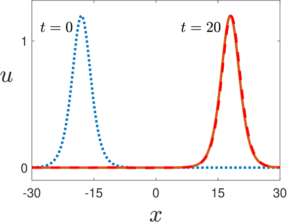
using the Matlab ODE solver ode45. Here the computational domain is taken as while the grid spacing is chosen as for which . In Figure 1 we plot the exact and numerical solutions at together with the initial state. The numerical solution has the same amplitude and waveform as that of the exact solution and overall there is a very good agreement between the two curves. This numerical experiment further verifies that the proposed semi-discrete scheme is capable of solving (1.1) to high accuracy.
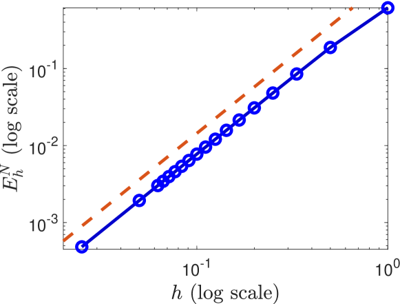
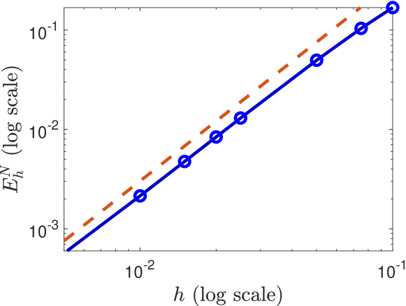
In order to verify the convergence rate estimate derived in Theorem 4.2 for the discretization error we now conduct a sequence of numerical experiments with different mesh sizes. Figure 2 shows the variation of the error measured using (6.1) with the mesh size. The computational domain is chosen large enough such that the discretization error () dominates the truncation error (). The figure has logarithmic scales on both axes and the dashed line corresponding to the theoretical quadratic convergence in space is also displayed for comparison. From the figure, one can observe that the numerical experiments provide a confirmation of the quadratic convergence rate predicted by Theorem 4.2.
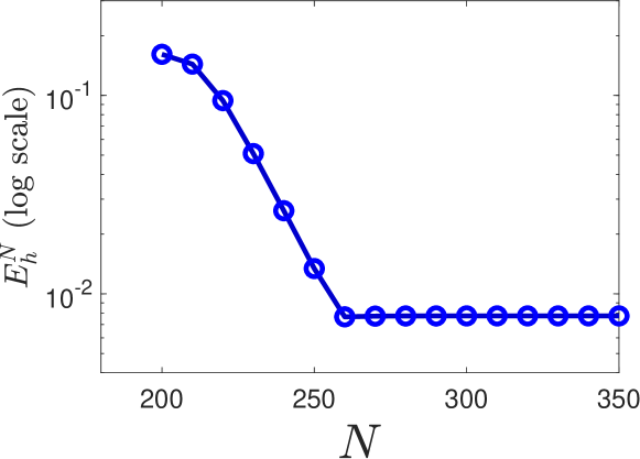
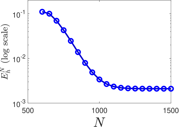
In another set of the numerical experiments we aim to show that, for sufficiently large values of , the truncation error due to the use of a finite number of grid points has no significant effect on the above numerical results. First, it is worth emphasizing that the solitary wave solution in (6.3) decays exponentially to zero for . Second, Example 5.6 shows that (recall that ). In the present set of the numerical experiments we fix the mesh size and vary the number of grid points, so the size of the computational domain is not the same for each experiment. However, by taking the initial condition and the time interval of the previous experiments and by taking sufficiently large , we guarantee that the wave dynamics occurs over a symmetric interval about the origin (with equidistant from both the left and right endpoints). The variation of the error at time with is shown in Figure 3 using a semi-logarithmic scale. We see that, up to a certain value of (), the truncation error dominates and it decreases exponentially as increases as indicated by . However, for larger values of , this phenomenon disappears and the discretization error dominates.
6.2 The Generalized Rosenau Equation
We continue our dicussion by considering the generalized Rosenau equation (1.4) which is a member of the class (1.1) with the kernel (1.3). In [9] it was pointed out that a particular solitary wave solution
| (6.5) |
with the constant wave speed , the width , the amplitude and the initial position satisfies the Rosenau equation (1.4) if the nonlinear term is in the form . It is worth mentioning that, contrary to the quadratic nonlinearity of the BBM equation, the Rosenau equation considered here has both cubic and quintic nonlinear terms. Consequently, a high resolution enhanced by a smaller mesh size is needed to achieve the same order of accuracy.
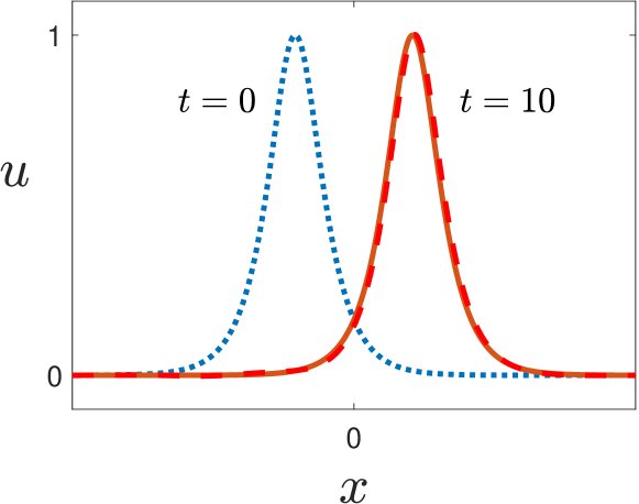
Generally, we follow closely what was done in the previous subsection for the BBM equation. Now, the initial condition is set to and (5.1) is solved up to time over the computational domain corresponding to (). In Figure 4 the numerical and exact solutions at are demonstrated and we see they agree very well.
To verify the quadratic convergence rate in space we now repeat the same numerical experiment with different values of (or equivalently with different values of ). On a logarithmic scale, Figure 5 displays the variation of the -error at time with the mesh size (again together with the dashed line of the theoretical quadratic convergence rate for comparison purposes). The computational results in Figure 5 are very similar to those shown in Figure 2 and they again verify the quadratic rate of convergence claimed in Theorem 4.2 for the discretization error.
In another set of numerical experiments for the Rosenau equation we investigate how the finite number of grid points affects the error. As for the BBM equation, this is done by fixing the mesh size, , and increasing until the error does not decrease anymore, i.e., until the error is nearly identical to the discretization error. In Figure 6, we plot, on a semi-logarithmic scale, the numerical results for the -error at time with . The figure shows that the error decreases exponentially for the relatively small values of while the relatively large values of have no major influence on the error. Recalling that the solitary wave solution in (6.5) decays exponentially to zero for and the expectation obtained from Example 5.7, one can conclude that these numerical experiments validate the theoretical results. Also, it is worth mentioning that the above results obtained for the Rosenau equation are qualitatively similar to those obtained for the BBM equation.
References
- [1] T. B. Benjamin, J. L. Bona, and J. J. Mahony. Model equations for long waves in nonlinear dispersive systems. Philos. Trans. R. Soc. Lond. Ser. A: Math. Phys. Sci., 272:47–78, 1972.
- [2] P. Rosenau. Dynamics of dense discrete systems: High order effects. Prog. Theor. Phys., 79:1028–1042, 1988.
- [3] H. Borluk and G. M. Muslu. Numerical solution for a general class of nonlocal nonlinear wave equations arising in elasticity. ZAMM-Z. Angew. Math. Mech., 97:1600–1610, 2017.
- [4] H. A. Erbay, S. Erbay, and A. Erkip. Convergence of a semi-discrete numerical method for a class of nonlocal nonlinear wave equations. ESAIM: Math. Model. Numer. Anal., 52:803–826, 2018.
- [5] J. L. Bona, W. G. Pritchard, and L. R. Scott. An evaluation of a model equation water waves. Philos. Trans. R. Soc. Lond. Ser. A: Math. Phys. Sci., 302:457–510, 1981.
- [6] N. Duruk, H. A. Erbay, and A. Erkip. Global existence and blow-up for a class of nonlocal nonlinear Cauchy problems arising in elasticity. Nonlinearity, 23:107–118, 2010.
- [7] A. Constantin and L. Molinet. The initial value problem for a generalized Boussinesq equation. Differential and Integral Equations, 15:1061–1072, 2002.
- [8] J. L. Bona, W. R. McKinney, and J. M. Restrepo. Stable and unstable solitary-wave solutions of the generalized regularized long-wave equation. J. Nonlinear Sci., 10:603–638, 2000.
- [9] M. A. Park. Pointwise decay estimates of solutions of the generalized Rosenau equation. J. Korean Math., 29:261–280, 1992.