Continuum model for relaxed twisted bilayer graphenes and moiré electron-phonon interaction

Abstract

We construct an analytic continuum model to describe the electronic structure and the electron-phonon interaction in twisted bilayer graphenes with arbitrary lattice deformation. Starting from the tight-binding model, we derive the interlayer Hamiltonian in the presence of general lattice displacement, and obtain a long-wavelength continuum expression for smooth deformation. We show that the continuum model correctly describes the band structures of the lattice-relaxed twisted bilayer graphenes. We apply the formula to the phonon vibration, and derive an explicit expression of the electron-phonon matrix elements between the moiré band states and the moiré phonon modes. By numerical calculation, we find that the electron-phonon coupling and phonon mediated electron-electron interaction are significantly enhanced in low twist angles due to the superlattice hybridization.

I Introduction

Twisted bilayer graphene (TBG) is a rotationaly-stacked graphene bilayer system governed by a nanoscale moiré interference pattern between the mismatched layers. Lopes dos Santos et al. (2007); Mele (2010); Trambly de Laissardière et al. (2010); Shallcross et al. (2010); Morell et al. (2010); Bistritzer and MacDonald (2011); Kindermann and First (2011); Xian et al. (2011); Lopes dos Santos et al. (2012); Moon and Koshino (2012); de Laissardiere et al. (2012) The physical properties of TBG are sensitive to lattice distortion, because a slight change in the atomic lattice is magnified to a big deformation in the moiré pattern, resulting in a significant influence on the electronic system. The actual atomic configuration of the real TBG is not a simple stack of rigid graphene layers, but it contains a triangular AB/BA-stacking domain structure as a consequence of spontaneous lattice relaxation. Popov et al. (2011); Brown et al. (2012); Lin et al. (2013); Alden et al. (2013); Uchida et al. (2014); van Wijk et al. (2015); Dai et al. (2016); Jain et al. (2016); Nam and Koshino (2017); Carr et al. (2018); Lin et al. (2018); Yoo et al. (2019); Guinea and Walet (2019). Such a structural deformation strongly affects the electronic band structure. Nam and Koshino (2017); Lin et al. (2018); Koshino et al. (2018); Yoo et al. (2019); Guinea and Walet (2019); Lucignano et al. (2019),

The moiré pattern plays an important role also in the lattice vibration. While the wide-range phonon spectrum of TBG resembles that of regular AB-stacked bilayer graphene Jiang et al. (2012); Cocemasov et al. (2013); Ray et al. (2016); Choi and Choi (2018), the detailed phonon structure is actually subject to a significant influence from the moiré effect. Angeli et al. (2019); Koshino and Son (2019) In the low-energy acoustic branch, in particular, the phonon spectrum is reconstructed into superlattice minibands ruled by the moiré period, where the eigen phonon modes can be regarded as effective vibration modes of the triangular domain structure. Koshino and Son (2019) These moiré phonon modes are expected to strongly interact with the flat band electronic states and affect the correlated phenomena. Cao et al. (2018a, b); Yankowitz et al. (2019) The electron-phonon interaction in TBG is theoretically studied by considering bare phonons without superlattice modulation Ray et al. (2016); Choi and Choi (2018); Wu et al. (2018, 2019); Lian et al. (2019), while the effect of the reconstructed moiré phonon modes is not well understood.

The purpose of this work is to develop a general continuum model for TBG with arbitrary lattice deformation, including lattice relaxation and phonon vibrations. The electronic properties of TBGs have been mostly studied by the continuum model, Lopes dos Santos et al. (2007); Bistritzer and MacDonald (2011); Kindermann and First (2011); Lopes dos Santos et al. (2012); Moon and Koshino (2013); Koshino (2015); Koshino and Moon (2015); Weckbecker et al. (2016) which can efficiently describe the band structure by capturing the long-wave components. However, the continuum model was originally derived for rigid TBGs, and the extension to deformed TBGs is necessary to study the above issues. Inclusion of the relaxation effect in the continuum model has been considered in very recent works. Koshino et al. (2018); Carr et al. (2019); Guinea and Walet (2019); Fang et al. (2019); Fleischmann et al. (2019); Balents (2019); Ochoa (2019)

In this paper, we construct an analytic continuum Hamiltonian for TBGs under arbitrary lattice deformation. Starting from the tight-binding model, we derive the interlayer Hamiltonian matrix as an analytic function of lattice displacement vectors. We then apply the continuum model to the relaxed TBGs with domain structureNam and Koshino (2017), and demonstrate the energy band of the original tight-binding model is correctly reproduced. Lastly we apply the formula to the phonon vibration, and obtain the electron-phonon matrix elements for the moiré phonon modes in relaxed TBGs.

The paper is organized as follows. In Sec. II, we present a general theoretical treatment to describe the electronic coupling between deformed graphene layers, and write down the interlayer matrix elements for arbitrary lattice displacement [Eq. (10)]. We then obtain its long-wavelength expression in a simple form [Eq. (22)], which is valid for small twist angles and smooth deformation. In Sec. III, we apply the continuum Hamiltonian to relaxed TBGs and calculate the band structure. In Sec. IV, we derive the quantized Hamiltonian for the lattice vibration of the relaxed TBG, and then obtain the explicit formula for the matrix elements between the electrons and the quantized moiré phonons.

II Continuum Hamiltonian of TBG with lattice deformation

II.1 Lattice geometry

Let us consider a TBG with twist angle $\theta$, and define its non-distorted structure by bilayer of intrinsic monolayer graphenes stacked with the graphite’s interlayer spacing $d_{0}=0.335$nm and in-plane rotation by $\mp\theta/2$ for layer 1 and 2, respectively. We take $x,y$ axes on the graphene layer, and $z$ axis perpendicular to it. The primitive lattice vectors of layer 1 is defined by $\mathbf{a}^{(1)}_{i}=R(-\theta/2)\mathbf{a}_{i}$ and those of layer 2 by $\mathbf{a}^{(2)}_{i}=R(\theta/2)\mathbf{a}_{i}$ ($i=1,2$), where $\mathbf{a}_{1}=a(1,0)$ and $\mathbf{a}_{2}=a(1/2,\sqrt{3}/2)$ are the lattice vectors before the rotation, $a\approx 0.246\,\mathrm{nm}$ is the graphene’s lattice constant, and $R$ is the rotation matrix. The unit cell area of monolayer graphene is given by $S_{0}=|\mathbf{a}_{1}\times\mathbf{a}_{2}|$. The primitive reciprocal lattice vectors of layer $l$ are $\mathbf{a}_{i}^{*(l)}=R(\mp\theta/2)\mathbf{a}^{*}_{i}$, where $\mathbf{a}^{*}_{1}=(2\pi/a)(1,-1/\sqrt{3})$ and $\mathbf{a}^{*}_{2}=(2\pi/a)(0,2/\sqrt{3})$ are those for non-rotated graphene.

Each graphene layer contains two sublattices labeled by $X=A,B$ in its own unit cell. In the absence of the lattice distortion, the positions of sublattice $X$ on layer $l$ are given by

$$\mathbf{R}^{(l)}_{X}=m_{1}\mathbf{a}^{(l)}_{1}+m_{2}\mathbf{a}^{(l)}_{2}+\mbox{\boldmath$\tau$}^{(l)}_{X}$$ (1)

Here $m_{1}$ and $m_{2}$ are integers, and $\mbox{\boldmath$\tau$}^{(l)}_{X}$ is the relative sublattice position inside the unit cell, which are given by $\mbox{\boldmath$\tau$}^{(1)}_{A}=0$, $\mbox{\boldmath$\tau$}^{(1)}_{B}=(\mathbf{a}^{(1)}_{1}-2\mathbf{a}^{(1)}_{2})/3$, $\mbox{\boldmath$\tau$}^{(2)}_{A}=d_{0}\,\mathbf{e}_{z}$ and $\mbox{\boldmath$\tau$}^{(2)}_{B}=(\mathbf{a}^{(2)}_{1}-2\mathbf{a}^{(2)}_{2})/3+d_{0}\,\mathbf{e}_{z}$. Here $\mathbf{e}_{z}$ is the unit vector in $z$ direction, and $d_{0}$ is the interlayer spacing in the absence of distortion, which is set to the interlayer distance of graphite, 0.334nm.

In a small angle TBG, a slight mismatch of the lattice periods gives rise to a moiré interference pattern. The reciprocal lattice vectors for the moiré pattern is given by $\mathbf{G}^{\rm M}_{i}=\textbf{a}^{*(1)}_{i}-\textbf{a}^{*(2)}_{i}\,(i=1,2).$ The real-space lattice vectors $\mathbf{L}^{\rm M}_{j}$ can be obtained from $\mathbf{G}^{\rm M}_{i}\cdot\mathbf{L}^{\rm M}_{j}=2\pi\delta_{ij}$. The moiré lattice constant $L_{\rm M}=|\mathbf{L}^{\rm M}_{i}|$ is given by $L_{\rm M}=a/[2\sin(\theta/2)]$. Figure 1(a) shows the folding of the Brillouin zone, where two large hexagons represent the first Brillouin zones of layer 1 and 2, and the small hexagon is the moiré Brillouin zone of TBG. The graphene’s Dirac points (the band touching points) are located at $\mathbf{K}^{(l)}_{\xi}=R(\mp\theta/2)\mathbf{K}_{\xi}$ with $\mp$ for layer 1 and 2, respectively, where $\mathbf{K}_{\xi}=-\xi[2\mathbf{a}^{*}_{1}+\mathbf{a}^{*}_{2}]/3=-\xi(2\pi/a)(2/3,0)$ is the Dirac points before rotation and $\xi=\pm 1$ is the valley index. In a small twist angle, $\mathbf{K}^{(1)}_{\xi}$ and $\mathbf{K}^{(2)}_{\xi}$ of the same valley $\xi$ are displaced only by a short distance of the order of $\mathbf{G}_{i}^{M}$.

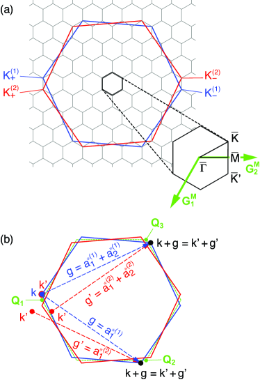
Figure 1: (a) Brillouin zone folding in TBG with $\theta=9.43^{\circ}$. Two large hexagons represent the first Brillouin zones of graphene layer 1 and 2, and the small hexagon is the moiré Brillouin zone of TBG. (b) Schematic diagram to illustrate the interlayer coupling from an initial $\mathbf{k}$ of layer 1(taken as $\mathbf{K}^{(1)}_{+}$) to three $\mathbf{k}^{\prime}$ points of layer 2 in a non-distorted TBG (see the text).

II.2 Interlayer Hamiltonian under general lattice distortion

Here we derive the general formula, Eq. (10), which describes the interlayer coupling between the Bloch states in TBG in the presence of arbitrary lattice distortion. We define $\mathbf{u}_{X}^{(l)}(\mathbf{R})$ as displacement vector of an atomic site of sublattice $X$ on layer $l$, which is originally located $\mathbf{R}(\in\mathbf{R}^{(l)}_{X})$. The $\mathbf{u}_{X}^{(l)}$ can be a three-dimensional vector in general. We expand the displacement vector in the Fourier series as

$$\mathbf{u}_{X}^{(l)}(\mathbf{R})=\sum_{\mathbf{q}}\mathbf{u}^{(l)}_{X,\mathbf{q}}e^{i\mathbf{q}\cdot\mathbf{R}},$$ (2)

where the summation in $\mathbf{q}$ is taken over two-dimensional wave numbers.

Let $|\mathbf{R}\rangle$ be a carbon $p_{z}$ orbital at site $\mathbf{R}$. We define the Bloch bases under the lattice distortion as

$$|\mathbf{k},X,l\rangle\equiv\frac{1}{\sqrt{N}}\sum_{\mathbf{R}\in\mathbf{R}^{(l)}_{X}}e^{i\mathbf{k}\cdot\mathbf{R}}|\mathbf{R}+\mathbf{u}_{X}^{(l)}(\mathbf{R})\rangle$$ (3)

where $\mathbf{k}$ is a two-dimensional Bloch wave vector, and $N=S/S_{0}$ is the number of graphene’s unit cells per layer in the total system area $S$. We assume the interlayer hopping from $|\mathbf{R}^{(1)}\rangle$ to $|\mathbf{R}^{(2)}\rangle$ is given by

$$\langle\mathbf{R}^{(2)}|U|\mathbf{R}^{(1)}\rangle=-T(\mathbf{R}^{(2)}-\mathbf{R}^{(1)}),$$ (4)

and define the three-dimensional Fourier transform as

$$t(\mathbf{p})=\frac{1}{S_{0}d_{0}}\int d^{3}r\,\,\,T(\mathbf{r})e^{-i\mathbf{p}\cdot\mathbf{r}},$$ (5)

where $\mathbf{p}=(p_{x},p_{y},p_{z})$ is a three dimensional wave vector.

In the actual band calculation in Sec. III, we will use the standard Slater-Koster form for $T(\mathbf{R})$,

$$-T(\mathbf{R})=V_{pp\pi}\left[1-\left(\frac{\mathbf{R}\cdot\mathbf{e}_{z}}{R}\right)^{2}\right]+V_{pp\sigma}\left(\frac{\mathbf{R}\cdot\mathbf{e}_{z}}{R}\right)^{2},$$

$$V_{pp\pi}=V_{pp\pi}^{0}e^{-(R-a_{0})/r_{0}},\,\,V_{pp\sigma}=V_{pp\sigma}^{0}e^{-(R-d_{0})/r_{0}}.$$ (6)

Here $\mathbf{e}_{z}$ is the unit vector perpendicular to the graphene plane, $a_{0}=a/\sqrt{3}\approx 0.142\,\mathrm{nm}$ is the distance of neighboring $A$ and $B$ sites, and the parameter $V_{pp\pi}^{0}\approx-2.7\,\mathrm{eV}$ is the transfer integral between the nearest-neighbor atoms on graphene, and $V_{pp\sigma}^{0}\approx 0.48\,\mathrm{eV}$ is the transfer integral between vertically located atoms on the neighboring layers of graphite, $r_{0}=0.184a$ is the decay length of the transfer integral. Moon and Koshino (2013)

The interlayer matrix element between the Bloch bases is written as

$$\langle\mathbf{k}^{\prime},X^{\prime},2|U|\mathbf{k},X,1\rangle$$

$$=-\frac{1}{N}\sum_{\mathbf{R}\in\mathbf{R}^{(1)}_{X}}\sum_{\mathbf{R}^{\prime}\in\mathbf{R}^{(2)}_{X^{\prime}}}\,e^{i\mathbf{k}\cdot\mathbf{R}-i\mathbf{k}^{\prime}\cdot\mathbf{R}^{\prime}}$$

$$\qquad\quad\times T[\mathbf{R}^{\prime}+\mathbf{u}_{X^{\prime}}^{(2)}(\mathbf{R}^{\prime})-\mathbf{R}-\mathbf{u}_{X}^{(1)}(\mathbf{R})]$$

$$=-\frac{1}{N}\frac{S_{0}d_{0}}{(2\pi)^{3}}\int d^{3}p\,\,t(\mathbf{p})\sum_{\mathbf{R}\in\mathbf{R}^{(1)}_{X}}e^{i(\mathbf{k}-\mathbf{p})\cdot\mathbf{R}-i\mathbf{p}\cdot\mathbf{u}_{X}^{(1)}(\mathbf{R})}$$

$$\qquad\qquad\qquad\times\sum_{\mathbf{R}^{\prime}\in\mathbf{R}^{(2)}_{X^{\prime}}}e^{-i(\mathbf{k}^{\prime}-\mathbf{p})\cdot\mathbf{R}^{\prime}+i\mathbf{p}\cdot\mathbf{u}_{X^{\prime}}^{(2)}(\mathbf{R}^{\prime})}.$$ (7)

We replace $\mathbf{u}_{X}^{(1)}(\mathbf{R})$ and $\mathbf{u}_{X^{\prime}}^{(2)}(\mathbf{R}^{\prime})$ with its Fourier transform in Eq. (2), and expand the exponential functions such as $\exp(i\mathbf{p}\cdot\mathbf{u}_{\mathbf{q}}e^{i\mathbf{q}\cdot\mathbf{R}})$ in a Taylor series as

$$\exp(i\mathbf{p}\cdot\mathbf{u}_{\mathbf{q}}\,e^{i\mathbf{q}\cdot\mathbf{R}})=\sum_{n=0}^{\infty}\frac{1}{n!}(i\mathbf{p}\cdot\mathbf{u}_{\mathbf{q}})^{n}e^{in\mathbf{q}\cdot\mathbf{R}}.$$ (8)

Then we can take the summation over the lattice points by using

$$\sum_{\mathbf{R}\in\mathbf{R}^{(l)}_{X}}e^{i\mathbf{p}\cdot\mathbf{R}}=N\sum_{\mathbf{g}}e^{i(\mathbf{g}+p_{z}\mathbf{e}_{z})\cdot\mbox{\boldmath\scriptsize$\tau$}^{(l)}_{X}}\delta_{\mathbf{p}_{\parallel},\mathbf{g}},$$ (9)

where $\mathbf{p}_{\parallel}$ is $xy$-component of $\mathbf{p}$, and the summation in $\mathbf{g}$ is taken over all the reciprocal lattice vectors $\mathbf{g}=m_{1}\mathbf{a}^{*(l)}_{1}+m_{2}\mathbf{a}^{*(l)}_{2}$.

Using these, we obtain a formula

$$\langle\mathbf{k}^{\prime},X^{\prime},2|U|\mathbf{k},X,1\rangle$$

$$=\sum_{\mathbf{g},\mathbf{g}^{\prime}}\sum_{n_{1},n_{2},\cdots}\sum_{n^{\prime}_{1},n^{\prime}_{2},\cdots}\Gamma_{(n_{1},n_{2},\cdots)}^{(n^{\prime}_{1},n^{\prime}_{2},\cdots)}(\mathbf{Q})\,\,e^{-i\mathbf{g}\cdot\mbox{\boldmath\scriptsize$\tau$}^{(1)}_{X}+i\mathbf{g}^{\prime}\cdot\mbox{\boldmath\scriptsize$\tau$}^{(2)}_{X^{\prime}}}$$

$$\qquad\times\delta_{\mathbf{k}+\mathbf{g}+n_{1}\mathbf{q}_{1}+n_{2}\mathbf{q}_{2}+\cdots,\,\mathbf{k}^{\prime}+\mathbf{g}^{\prime}-n^{\prime}_{1}\mathbf{q}_{1}-n^{\prime}_{2}\mathbf{q}_{2}+\cdots},$$ (10)

where $\mathbf{g}=m_{1}\mathbf{a}^{*(1)}_{1}+m_{2}\mathbf{a}^{*(1)}_{2}$ and $\mathbf{g}^{\prime}=m^{\prime}_{1}\mathbf{a}^{*(2)}_{1}+m^{\prime}_{2}\mathbf{a}^{*(2)}_{2}$, $n_{i},n^{\prime}_{i}=0,1,2,\cdots$, $\mathbf{Q}=\mathbf{k}+\mathbf{g}+n_{1}\mathbf{q}_{1}+n_{2}\mathbf{q}_{2}+\cdots$, and

$$\Gamma_{(n_{1},n_{2},\cdots)}^{(n^{\prime}_{1},n^{\prime}_{2},\cdots)}(\mathbf{Q})=-\frac{d_{0}}{2\pi}\int_{-\infty}^{\infty}dp_{z}t(\mathbf{Q}^{\prime})e^{ip_{z}d_{0}}$$

$$\quad\times\frac{[-i\mathbf{Q}^{\prime}\cdot\mathbf{u}^{(1)}_{X,\mathbf{q}_{1}}]^{n_{1}}}{n_{1}!}\frac{[-i\mathbf{Q}^{\prime}\cdot\mathbf{u}^{(1)}_{X,\mathbf{q}_{2}}]^{n_{2}}}{n_{2}!}\cdots$$

$$\quad\times\frac{[+i\mathbf{Q}^{\prime}\cdot\mathbf{u}^{(2)}_{X^{\prime},\mathbf{q}_{1}}]^{n^{\prime}_{1}}}{n^{\prime}_{1}!}\frac{[+i\mathbf{Q}^{\prime}\cdot\mathbf{u}^{(2)}_{X^{\prime},\mathbf{q}_{2}}]^{n^{\prime}_{2}}}{n^{\prime}_{2}!}\cdots,$$ (11)

with $\mathbf{Q}^{\prime}=\mathbf{Q}+p_{z}\mathbf{e}_{z}$. Here $\{\mathbf{q}_{1},\mathbf{q}_{2},\cdots\}$ is a set of the two-dimensional wave numbers in which $\mathbf{u}^{(l)}_{X,\mathbf{q}}$ has finite Fourier amplitudes. Eq. (10) simply means that the Bloch states of the layer 1 and layer 2 are coupled when

$$\mathbf{k}+\mathbf{g}+n_{1}\mathbf{q}_{1}+n_{2}\mathbf{q}_{2}+\cdots$$

$$\quad=\mathbf{k}^{\prime}+\mathbf{g}^{\prime}-n^{\prime}_{1}\mathbf{q}_{1}-n^{\prime}_{2}\mathbf{q}_{2}+\cdots(=\mathbf{Q}),$$ (12)

and its coupling amplitude is given by $\Gamma_{(n_{1},n_{2},\cdots)}^{(n^{\prime}_{1},n^{\prime}_{2},\cdots)}(\mathbf{Q})$. The higher order terms in $n_{i}$ and $n^{\prime}_{i}$ in Eq. (11) quickly decay as long as $|\mathbf{Q}^{\prime}\cdot\mathbf{u}^{(l)}_{X,\mathbf{q}_{j}}|$ is sufficiently small, and it is the case in TBGs considered below.

When the displacement vector is along in-plane direction (i.e., $u_{z}^{(l)}=0$), in particular, Eq. (11) is reduced to

$$\Gamma_{(n_{1},n_{2},\cdots)}^{(n^{\prime}_{1},n^{\prime}_{2},\cdots)}(\mathbf{Q})=-t_{\parallel}(\mathbf{Q};\,d_{0})$$

$$\quad\times\frac{[-i\mathbf{Q}\cdot\mathbf{u}^{(1)}_{X,\mathbf{q}_{1}}]^{n_{1}}}{n_{1}!}\frac{[-i\mathbf{Q}\cdot\mathbf{u}^{(1)}_{X,\mathbf{q}_{2}}]^{n_{2}}}{n_{2}!}\cdots$$

$$\quad\times\frac{[+i\mathbf{Q}\cdot\mathbf{u}^{(2)}_{X^{\prime},\mathbf{q}_{1}}]^{n^{\prime}_{1}}}{n^{\prime}_{1}!}\frac{[+i\mathbf{Q}\cdot\mathbf{u}^{(2)}_{X^{\prime},\mathbf{q}_{2}}]^{n^{\prime}_{2}}}{n^{\prime}_{2}!}\cdots,$$ (13)

where

$$t_{\parallel}(\mathbf{Q};\,z) =\frac{d_{0}}{2\pi}\int_{-\infty}^{\infty}dp_{z}\,\,t(\mathbf{Q}+p_{z}\mathbf{e}_{z})e^{ip_{z}z}$$

$$=\frac{1}{S_{0}}\int d^{2}r\,\,T(\mathbf{r}+z\mathbf{e}_{z})e^{-i\mathbf{Q}\cdot\mathbf{r}},$$ (14)

is the two-dimensional Fourier transform of $T(\mathbf{r})$ on a plane parallel to $xy$ at fixed height $z$.

In the absence of the displacement (i.e., $\mathbf{u}^{(l)}_{X}=0$), the terms in the Taylor series remain only when $n_{j}=n^{\prime}_{j}=0$, and Eq. (10) becomes

$$\langle\mathbf{k}^{\prime},X^{\prime},2|U|\mathbf{k},X,1\rangle$$

$$=-\sum_{\mathbf{g},\mathbf{g}^{\prime}}t_{\parallel}(\mathbf{k}+\mathbf{g};\,d_{0})\,e^{-i\mathbf{g}\cdot\mbox{\boldmath\scriptsize$\tau$}^{(1)}_{X}+i\mathbf{g}^{\prime}\cdot\mbox{\boldmath\scriptsize$\tau$}^{(2)}_{X^{\prime}}}\delta_{\mathbf{k}+\mathbf{g},\mathbf{k}^{\prime}+\mathbf{g}^{\prime}},$$ (15)

which is the interlayer Hamiltonian of non-distorted TBG in the earlier works. Bistritzer and MacDonald (2011); Koshino (2015)

II.3 Continuum Hamiltonian for small twist angles

Eq. (10) is the general formula which works for any twist angles with arbitrary displacement vectors. Here we will derive a long-range approximate form, Eq. (22), which is valid for small twist angles and long-range displacement. In the following, we assume that the moiré period much greater than the atomic scale, and also that $\textbf{u}^{(l)}_{A}(\mathbf{r})=\textbf{u}^{(l)}_{B}(\mathbf{r})=\textbf{u}^{(l)}(\mathbf{r})$, where $\textbf{u}^{(l)}$ is a smoothly varying function compared to the atomic scale.

We first consider the non-distorted case, $\mathbf{u}^{(l)}=0$. In Eq. (15), the Bloch states at $\mathbf{k}$ (layer 1) and $\mathbf{k}^{\prime}$ (layer 2) are mixed when $\mathbf{k}+\mathbf{g}=\mathbf{k}^{\prime}+\mathbf{g}^{\prime}$, and then the coupling amplitude is given by $t_{\parallel}(\mathbf{k}+\mathbf{g};\,d_{0})$. Here only a few terms are relevant in the summation over $\mathbf{g}$ and $\mathbf{g}^{\prime}$, because the function $t_{\parallel}(\mathbf{k}+\mathbf{g};\,d_{0})$ quickly decays for large $|\mathbf{k}+\mathbf{g}|$. When we start from $\mathbf{k}\approx\mathbf{K}_{\xi}$ to consider a low-energy state near the Fermi energy, the dominant coupling occurs in three cases $(\mathbf{g},\mathbf{g}^{\prime})=(\mathbf{0},\mathbf{0}),\xi(\mathbf{a}^{*(1)}_{1},\mathbf{a}^{*(2)}_{1}),\xi(\mathbf{a}^{*(1)}_{1}+\mathbf{a}^{*(1)}_{2},\mathbf{a}^{*(2)}_{1}+\mathbf{a}^{*(2)}_{2})$. Figure 1(b) shows the positions of $\mathbf{k}$, $\mathbf{k}^{\prime}$ and $\mathbf{k}+\mathbf{g}$ for an initial vector $\mathbf{k}=\mathbf{K}^{(1)}_{+}$. The corresponding $\mathbf{k}+\mathbf{g}$ is close to three equivalent corner points of the first Brillouin zone of non-rotated graphene,

$$\mathbf{Q}_{1}=\mathbf{K}_{\xi},\,\,\mathbf{Q}_{2}=\mathbf{K}_{\xi}+\xi\mathbf{a}^{*}_{1},\,\,\mathbf{Q}_{3}=\mathbf{K}_{\xi}+\xi(\mathbf{a}^{*}_{1}+\mathbf{a}^{*}_{2}).$$ (16)

By neglecting a small shift, we can replace $\mathbf{k}+\mathbf{g}$ with $\mathbf{Q}_{j}$ in $t_{\parallel}(\mathbf{k}+\mathbf{g};\,d_{0})$ of Eq. (15). This gives the widely-used continuum model for the non-distorted TBG. Bistritzer and MacDonald (2011)

The same approximation can be used in the presence of a long-range lattice distortion $\mathbf{u}^{(l)}$. When $\mathbf{q}$’s in $\mathbf{u}^{(l)}_{\mathbf{q}}$ are much shorter than $1/a$ (i.e., $\mathbf{u}^{(l)}(\mathbf{r})$ is smoothly varying compared to $a$), we can neglect a small shift $n_{1}\mathbf{q}_{1}+n_{2}\mathbf{q}_{2}+\cdots$ in $\mathbf{Q}$ in the coupling amplitude $\Gamma_{(n_{1},n_{2},\cdots)}^{(n^{\prime}_{1},n^{\prime}_{2},\cdots)}(\mathbf{Q})$. Then we can replace $\mathbf{Q}$ with the above three $\mathbf{Q}_{j}$’s in Eq. (10) to obtain,

$$\langle\mathbf{k}^{\prime},X^{\prime},2|U|\mathbf{k},X,1\rangle$$

$$\qquad=\sum_{j=1}^{3}\sum_{n_{1},n_{2},\cdots}\sum_{n^{\prime}_{1},n^{\prime}_{2},\cdots}\Gamma_{(n_{1},n_{2},\cdots)}^{(n^{\prime}_{1},n^{\prime}_{2},\cdots)}(\mathbf{Q}_{j})M^{j}_{X^{\prime}X}$$

$$\qquad\qquad\times\delta_{\mathbf{k}^{\prime},\mathbf{k}+\delta\mathbf{k}_{j}+(n_{1}+n^{\prime}_{1})\mathbf{q}_{1}+(n_{2}+n^{\prime}_{2})\mathbf{q}_{2}+\cdots},$$ (17)

where $\delta\mathbf{k}_{j}(=\mathbf{g}-\mathbf{g}^{\prime})$ is given by

$$\delta\mathbf{k}_{1}=\mathbf{0},\,\,\delta\mathbf{k}_{2}=\xi\mathbf{G}^{M}_{1},\,\,\delta\mathbf{k}_{2}=\xi(\mathbf{G}^{M}_{1}+\mathbf{G}^{M}_{2}),$$ (18)

and $M^{j}_{X^{\prime}X}(=e^{-i\mathbf{g}\cdot\mbox{\boldmath\scriptsize$\tau$}^{(1)}_{X}+i\mathbf{g}^{\prime}\cdot\mbox{\boldmath\scriptsize$\tau$}^{(2)}_{X^{\prime}}}$) is

$$M^{1}=\begin{pmatrix}1&1\\ 1&1\end{pmatrix},M^{2}=\begin{pmatrix}1&\omega^{-\xi}\\ \omega^{\xi}&1\end{pmatrix},\,\,M^{3}=\begin{pmatrix}1&\omega^{\xi}\\ \omega^{-\xi}&1\end{pmatrix},\,\,$$ (19)

where $\omega=e^{2\pi i/3}$ and $M^{j}$ stands for

$$M^{j}=\begin{pmatrix}M^{j}_{AA}&M^{j}_{AB}\\ M^{j}_{BA}&M^{j}_{BB}\end{pmatrix}.$$ (20)

In the real space representation, Eq. (17) is simply expressed as

$$\langle\mathbf{k}^{\prime},X^{\prime},2|U|\mathbf{k},X,1\rangle=\frac{1}{S}\int d^{2}re^{i(\mathbf{k}-\mathbf{k}^{\prime})\cdot\mathbf{r}}U_{X^{\prime}X}(\mathbf{r}),$$ (21)

where

$$U_{X^{\prime}X}(\mathbf{r})= -\sum_{j=1}^{3}M^{j}_{X^{\prime}X}\,\,t_{\parallel}[\mathbf{Q}_{j};d_{0}+u^{-}_{z}(\mathbf{r})]$$

$$\qquad\times\exp[i\mathbf{Q}_{j}\cdot\mathbf{u}^{-}(\mathbf{r})+i\delta\mathbf{k}_{j}\cdot\mathbf{r}].$$ (22)

where $\mathbf{u}^{-}=\mathbf{u}^{(2)}-\mathbf{u}^{(1)}$ is the interlayer asymmetric displacement vector between the two layers. From Eq. (17) to Eq. (22), we used $\delta_{\mathbf{k}^{\prime},\mathbf{k}+\mathbf{q}}=(1/S)\int d^{2}r\,e^{i(\mathbf{k}+\mathbf{q}-\mathbf{k}^{\prime})}$, and applied Eq. (8) inversely, and finally used Eq. (14) for the integral in $p_{z}$. Note that the interlayer Hamiltonian matrix of $U$ only depends on the asymmetric displacement $\mathbf{u}^{-}$, but not on the symmetric part $\mathbf{u}^{+}=\mathbf{u}^{(2)}+\mathbf{u}^{(1)}$.

In in-plane distortion (i.e., $u_{z}^{(l)}=0$), particularly, Eq. (22) becomes

$$U_{X^{\prime}X}(\mathbf{r})=t_{0}\sum_{j=1}^{3}M^{j}_{X^{\prime}X}\exp[i\mathbf{Q}_{j}\cdot\mathbf{u}^{-}(\mathbf{r})+i\delta\mathbf{k}_{j}\cdot\mathbf{r}],$$ (23)

where $t_{0}=-t_{\parallel}[\mathbf{Q}_{j};d_{0}].$ Note that $t_{0}$ is independent of $j$ because $|\mathbf{Q}_{1}|=|\mathbf{Q}_{2}|=|\mathbf{Q}_{3}|=4\pi/(3a)$, and $t_{\parallel}(\mathbf{q};d_{0})$ is circularly symmetric. In the present hopping model of Eq.  (6), we have $t_{0}=0.104$ eV.

The total continuum Hamiltonian of TBG for the valley $\xi$ can be written in a 4 $\times$ 4 matrix for the basis of $(A_{1},B_{1},A_{2},B_{2})$ as

$${H}=\begin{pmatrix}H_{1}&U^{\dagger}\\ U&H_{2}\end{pmatrix}.$$ (24)

Here $U$ is given by Eq. (22). The $H_{l}\,(l=1,2)$ is the intralayer Hamiltonian of layer $l$, which is given by the two-dimensional Weyl equation centered at $\mathbf{K}^{(l)}_{\xi}$ point,

$$H_{l}(\mathbf{k})=-\hbar v\left[R(\pm\theta/2)\left({\mathbf{k}}+\frac{e}{\hbar}\mathbf{A}^{(l)}-\mathbf{K}^{(l)}_{\xi}\right)\right]\cdot(\xi\sigma_{x},\sigma_{y}),$$ (25)

where $\pm$ is for $l=1$ and 2, respectively, $v$ is the graphene’s band velocity, and $\sigma_{x},\sigma_{y}$ are the Pauli matrices in the sublattice space $(A,B)$. We take $\hbar v/a=2.1354$ eV.Moon and Koshino (2013) The $\mathbf{A}^{(l)}$ is the pseudo-vector potential induced by the lattice strain, which given by Suzuura and Ando (2002); Pereira and Neto (2009); Guinea et al. (2010)

$$A^{(l)}_{x} = \xi\frac{3}{4}\frac{\beta\gamma_{0}}{ev}[u^{(l)}_{xx}-u^{(l)}_{yy}],$$

$$A^{(l)}_{y} = \xi\frac{3}{4}\frac{\beta\gamma_{0}}{ev}[-2u^{(l)}_{xy}].$$ (26)

where $u^{(l)}_{ij}=(\partial_{i}u_{j}^{(l)}+\partial_{j}u_{i}^{(l)})/2$ is strain tensor, $\gamma_{0}=|V_{pp\pi}^{0}|$ is the nearest neighbor transfer energy of intrinsic graphene, and

$$\beta=-\frac{d\ln T(\mathbf{r})}{d\ln r}\Bigr{|}_{r=a_{0}},$$ (27)

where $\mathbf{r}$ is on the $xy$-plane. In the present model Eq.  (6), we have $\beta=a_{0}/r_{0}\approx 3.14$. In the Fourier representation, Eq. (26) becomes

$$\mathbf{A}^{(l)}=\xi\frac{3}{4}\frac{\beta\gamma_{0}}{ev}\sum_{\mathbf{q}}\hat{W}_{\mathbf{q}}\mathbf{u}_{\mathbf{q}}^{(l)}e^{i\mathbf{q}\cdot\mathbf{r}},$$ (28)

where

$$\hat{W}_{\mathbf{q}}=\begin{pmatrix}iq_{x}&-iq_{y}\\ -iq_{y}&-iq_{x}\end{pmatrix}.$$ (29)

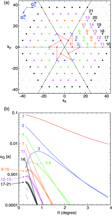
Figure 2: (a) The $k$-space map of the Fourier components $i\textbf{u}^{-}_{\textbf{G}}$ at $\theta=0.817^{\circ}$. The grid points represents G’s and the length of arrows is proportional to $|\textbf{u}^{-}_{\textbf{G}}|$. (b) Logarithmic plot of $|\textbf{u}^{-}_{\textbf{G}}|$ (in units of graphene’s lattice constant, $a$) as a function of the twist angle, where the numbers specify the different $\mathbf{G}$ vectors indicated in (a). Gray lines are for additional $\mathbf{G}$ vectors taken only for $\theta=0.3^{\circ}$ and 0.4^∘.

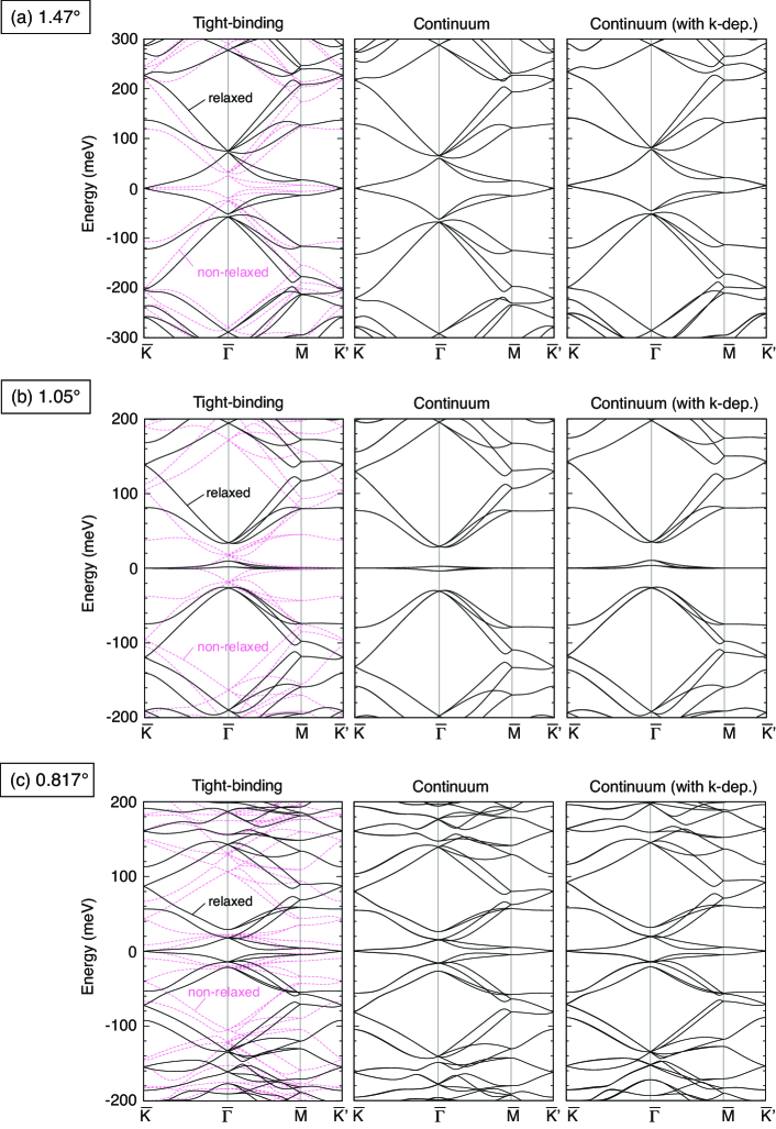
Figure 3: Band structure of relaxed TBGs of (a) $\theta=1.47^{\circ}$, (b) $1.05^{\circ}$, and (c) $0.817^{\circ}$. The left panel is calculated by the original tight-binding model, where dashed pink lines are the energy bands without lattice relaxation. The middle and right panels are by the continuum model with the constant interlayer matrix $U$ and that with a linear $\mathbf{k}$-dependence in $U$, respectively (see the text).

III Band structure of the relaxed TBG

Using the formula obtained above, we calculate the band structure of relaxed TBGs with the AB-BA domain wall formation. For the displacement vector, we use our previous calculation method Nam and Koshino (2017); Koshino and Son (2019) which considers only in-plane components, as the simplest approximation to describe the domain formation. Here $\mathbf{u}^{-}(\mathbf{r})$ is assumed to have the same periodicity as the original moiré pattern, or

$$\textbf{u}^{-}(\textbf{r})=\sum_{\textbf{G}}\textbf{u}^{-}_{\textbf{G}}e^{i\textbf{G}\cdot\textbf{r}},$$ (30)

where $\textbf{G}=m\textbf{G}^{\rm M}_{1}+n\textbf{G}^{\rm M}_{2}$ are moiré reciprocal vectors.

Figure 2(a) shows the $k$-space map of the Fourier components $i\textbf{u}^{-}_{\textbf{G}}$ at $\theta=0.817^{\circ}$, where the triangular grid presents the moiré reciprocal lattice points and the length of the arrows is proportional to $|\textbf{u}^{-}_{\textbf{G}}|$. The $\textbf{u}^{-}$ has six-fold rotational symmetry as assumed in the calculation, and its direction spirals around the origin. Figure 2(b) is a logarithmic plot of the absolute value $|\textbf{u}^{-}_{\textbf{G}}|$ as a function of the twist angle, where the numbers specify the different $\mathbf{G}$ vectors indicated in Fig. 2(a). In twist angles larger than $1^{\circ}$, the dominant contribution mostly comes from the shortest G (indicated by “1”). The higher harmonics becomes gradually relevant in $\theta<1^{\circ}$, where we see that the components at $\arctan(G_{y}/G_{x})=0^{\circ},60^{\circ},120^{\circ},\cdots$ have relatively larger amplitudes than other directions. We also found that, in any twist angles, $\textbf{u}^{-}_{\textbf{G}}$ and G are exactly perpendicular at the wave points with $\arctan(G_{y}/G_{x})=0^{\circ},30^{\circ},60^{\circ},\cdots$, and otherwise they are almost perpendicular with a few degree shift. In the calculation, we took 21 $\mathbf{G}$-points per 1/6 sector [i.e., $0\leq\arctan(G_{y}/G_{x})<60^{\circ}$] for twist angles $\theta>0.5^{\circ}$, and 36 points for the two smallest angles, $\theta=0.3^{\circ}$ and $0.4^{\circ}$.

Using the above $\textbf{u}^{-}$, the Hamiltonian for the relaxed TBG is obtained by using Eqs. (23) and (24). In the practical calculation, we expand $\exp[i\mathbf{Q}_{j}\cdot\mathbf{u}^{-}(\mathbf{r})]$ in Eq. (23) back to the $k$-space representation Eq. (17), and diagonalize the Hamiltonian in $k$-space bases. The matrix element is expressed in power of $|\mathbf{Q}_{j}\cdot\mathbf{u}^{-}_{\mathbf{G}}|$ as in Eq. (13), and the higher harmonics quickly decay provided that $|\mathbf{Q}_{j}\cdot\mathbf{u}^{-}_{\mathbf{G}}|$ is much smaller than 1. This condition is well satisfied in the twist angles studied here, since $|\mathbf{Q}_{j}|=4\pi/(3a)$ and $|\mathbf{u}^{-}_{\mathbf{G}}|<0.1a$ as seen in Fig. 2(b). Figure 3 presents the calculated band structures of relaxed TBGs at twist angles (a) 1.47^∘, (b) 1.05^∘, and (c) 0.817^∘. In each row, the left panel is the band structure calculated by the original tight-binding model with the hopping function of Eq. (6), where solid black and dashed pink lines are the energy bands with and without lattice relaxation, respectively, and we shifted the origin of the energy axis to the band touching points at $\bar{K}$ and $\bar{K}^{\prime}$. The middle panel presents the energy band of relaxed TBGs obtained by the continuum model of Eqs. (23) and (24).

We see a nice agreement between the tight-binding model and the continuum model, while also notice that a slight asymmetry between the electron side and hole side in the tight-binding result is ignored in the continuum model. Actually, it was recently shown that the electron-hole asymmetry can be taken into account by including $k$-linear term in the interlayer coupling. Carr et al. (2019); Fang et al. (2019); Guinea and Walet (2019) Our original expression for the interlayer matrix element Eq. (10) depends on the position of initial $\mathbf{k}$ through $\mathbf{Q}$, but the $\mathbf{k}$-dependence is dropped by replacing $\mathbf{Q}$ with constant $\mathbf{Q}_{j}$ in Eq. (23). In the right panels, we show the band structure calculated by the original Eq. (10) with $\mathbf{k}$-dependence included in the linear order, where we actually see that the electron-hole asymmetry is restored.

The role of the displacement vector can be understood by expanding the Hamiltonian in powers of the displacement vectors. Within the first order in $\mathbf{u}^{-}$, the interlayer matrix $U$ of Eq. (23) is written as

$$U_{X^{\prime}X}(\mathbf{r})\approx t_{0}\sum_{j=1}^{3}M^{j}_{X^{\prime}X}e^{i\delta\mathbf{k}_{j}\cdot\mathbf{r}}\Biggl{(}1+i\mathbf{Q}_{j}\cdot\sum_{\textbf{G}}\textbf{u}^{-}_{\textbf{G}}e^{i\textbf{G}\cdot\textbf{r}}\Biggr{)},$$ (31)

By only taking the six dominant components of $\mathbf{u}^{-}_{\mathbf{G}}$ [Fig. 2(a)], we have

$$U =\begin{pmatrix}U_{AA}&U_{AB}\\ U_{BA}&U_{BB}\end{pmatrix}$$

$$\approx\begin{pmatrix}t&t^{\prime}\\ t^{\prime}&t\end{pmatrix}+\begin{pmatrix}t&t^{\prime}\omega^{-\xi}\\ t^{\prime}\omega^{\xi}&t\end{pmatrix}e^{i\xi\mathbf{G}^{\rm M}_{1}\cdot\mathbf{r}}$$

$$\qquad+\begin{pmatrix}t&t^{\prime}\omega^{\xi}\\ t^{\prime}\omega^{-\xi}&t\end{pmatrix}e^{i\xi(\mathbf{G}^{\rm M}_{1}+\mathbf{G}^{\rm M}_{2})\cdot\mathbf{r}}+\cdots,$$ (32)

where

$$t=t_{0}(1-2\alpha),\quad t^{\prime}=t_{0}(1+\alpha/2),$$ (33)

$$\alpha=\frac{2\pi}{\sqrt{3}}\frac{u_{1}}{a},$$ (34)

and $u_{1}$ is the absolute value of the leading $\mathbf{u}^{-}_{\mathbf{G}}$, plotted as curve 1 in Fig. 2(b). We see that the in-plane distortion enhances the off-diagonal elements (AB and BA) while suppresses the diagonal elements (AA and BB) in the $U$ matrix. This is interpreted as a consequence of the lattice relaxation, which maximizes the AB/BA-stacking area while minimizes the unfavorable AA/BB-stacking area.

Interestingly, a similar Hamiltonian with $t<t^{\prime}$ was also obtained by considering the out-of-plane distortion only.Koshino et al. (2018) In this case, the diagonal terms is reduced because the interlayer spacing at $AA$ region is elongated and the local interlayer coupling is reduced. In the band structure, the difference between $t$ and $t^{\prime}$ is responsible for the gap opening between the flat band and the excited bandsKoshino et al. (2018); Tarnopolsky et al. (2019); Liu et al. (2019), and this is also true in the present case with the in-plane distortion, as shown in Fig. 3.

IV Electron-phonon interaction in the relaxed TBG

IV.1 Quantized moiré phonons in TBG

Here we derive the Hamiltonian of moiré acoustic phonons in the relaxed TBG, by quantizing the classical motion of the lattice vibration. Koshino and Son (2019) The interaction between the quantized phonons and the electronic system will be argued in the next subsection.

We consider a long-wave, in-plane lattice vibration specified by the displacement vector, $\textbf{u}^{(l)}_{A}=\textbf{u}^{(l)}_{B}=\textbf{u}^{(l)}(\textbf{r},t)$ for layer $l=1,2$. We again assume $u_{z}^{(l)}=0$. The Lagrangian of the system is given by $L=T-(U_{E}+U_{B})$ as a functional of $\textbf{u}^{(l)}$. The term $T$ is the kinetic energy due to the motion of the carbon atoms,

$$T=\sum_{l=1}^{2}\int\frac{\rho}{2}\left[\dot{u}_{x}^{(l)2}+\dot{u}_{y}^{(l)2}\right]d^{2}r,$$ (35)

where $\rho=7.61\times 10^{-7}$ kg/m² is the area density of single-layer graphene, and $\dot{u_{i}}$ represents the time derivative of $u_{i}$. The $U_{E}$ is the elastic energy of strained TBG given by Suzuura and Ando (2002); San-Jose et al. (2014)

$$U_{E}=\sum_{l=1}^{2}\int\frac{1}{2}\left\{(\lambda+\mu)(u_{xx}^{(l)}+u_{yy}^{(l)})^{2}\right.$$

$$\left.+\mu\left[(u_{xx}^{(l)}-u_{yy}^{(l)})^{2}+4(u_{xy}^{(l)})^{2}\right]\right\}d^{2}r,$$ (36)

where $\lambda\approx 3.25$ eV/$\text{\AA}^{2}$ and $\mu\approx 9.57$ eV/$\text{\AA}^{2}$ are graphene’s $\text{Lam}\acute{\text{e}}$ factors Zakharchenko et al. (2009); Jung et al. (2015), and $u^{(l)}_{ij}=(\partial_{i}u_{j}^{(l)}+\partial_{j}u_{i}^{(l)})/2$ is strain tensor. The $U_{B}$ is the registry-dependent inter-layer binding energy Nam and Koshino (2017); Koshino and Son (2019),

$$U_{B}=\int\text{d}^{2}r\,\sum^{3}_{j=1}2V_{0}\cos[\textbf{G}_{j}^{\rm M}\cdot\textbf{r}+\textbf{a}^{*}_{j}\cdot(\textbf{u}^{(2)}-\textbf{u}^{(1)})],$$ (37)

where $\textbf{a}^{*}_{3}=-\textbf{a}^{*}_{1}-\textbf{a}^{*}_{2}$, and $\textbf{G}^{\rm M}_{3}=-\textbf{G}^{\rm M}_{1}-\textbf{G}^{\rm M}_{2}$. The difference between the binding energies of AA and AB/BA structure is $9V_{0}$ per area, and this amounts to $\Delta\epsilon=9V_{0}S_{G}/4$ per atom where $S_{G}$ is the area of graphene’s unit cell. In the following calculation, we use $\Delta\epsilon=0.0189$ (eV/atom) as a typical value Lebedeva et al. (2011); Popov et al. (2011).

The Lagrangian $L$ can be separated into the interlayer symmetric part and asymmetric part, which are associated with $\textbf{u}^{\pm}=\textbf{u}^{(2)}\pm\textbf{u}^{(1)}$, respectively. Since the interlayer binding energy $U_{B}$ only depends on $\textbf{u}^{-}$, the moiré interlayer coupling only affects the motion of $\textbf{u}^{-}$ while leaving $\textbf{u}^{+}$ unchanged from the intrinsic graphene.Koshino and Son (2019) In the following, we only consider $\textbf{u}^{-}$ sector of the Lagrangian. We consider a small vibration around the relaxed state, i.e.,

$$\textbf{u}^{-}(\mathbf{r},t)=\textbf{u}^{-}_{0}(\mathbf{r})+\delta\textbf{u}^{-}(\mathbf{r},t).$$ (38)

Here $\textbf{u}^{-}_{0}(\mathbf{r})$ is the static relaxed state to minimize $U_{B}+U_{E}$, which was argued in Sec. III, and $\delta\textbf{u}^{-}(\mathbf{r},t)$ is a perturbational vibration around $\textbf{u}^{-}_{0}$. We define the Fourier transform

$$\textbf{u}_{0}^{-}(\textbf{r})=\sum_{\textbf{G}}\textbf{u}^{-}_{0,\textbf{G}}e^{i\textbf{G}\cdot\textbf{r}},$$ (39)

$$\delta\textbf{u}^{-}(\textbf{r},t)=\sqrt{\frac{1}{S}}\sum_{\textbf{q}}\delta\textbf{u}^{-}_{\textbf{q}}(t)e^{i\textbf{q}\cdot\textbf{r}},$$ (40)

where $\mathbf{G}=m_{1}\mathbf{G}^{M}_{1}+m_{2}\mathbf{G}^{M}_{2}$, and the factor $\sqrt{1/S}$ is required to normalize the phonon operators introduced later.

We rewrite the Lagrangian in terms of $\textbf{u}_{0}^{-}$ and $\delta\textbf{u}^{-}$, and expand it into a series of $\delta\textbf{u}^{-}$ within the second order. The relaxed state $\textbf{u}^{-}_{0}$ can be obtained by the variational principle $[\delta(U_{E}+U_{B})/\delta(\delta\textbf{u}^{-})]=0$. Nam and Koshino (2017) We introduce the canonical momentum

$$\delta\mathbf{p}^{-}_{\mathbf{q}}=\frac{\partial L}{\partial\delta\textbf{u}^{-}_{\mathbf{q}}}=\rho_{r}\,\delta\dot{\textbf{u}}^{-}_{-\mathbf{q}},$$ (41)

where

$$\rho_{r}=\frac{\rho}{2}$$ (42)

is the reduced mass for the relative motion. The Hamiltonian $H=\sum_{\mathbf{q}}\delta\mathbf{p}^{-}_{\mathbf{q}}\cdot\delta\textbf{u}^{-}_{\mathbf{q}}-L$ can be written as

$$H= \sum_{\mathbf{q}\in{\rm MBZ}}\Biggl{[}\sum_{\mathbf{G}}\frac{1}{2\rho_{r}}\delta\mathbf{p}^{-\dagger}_{\mathbf{q+\mathbf{G}}}\cdot\delta\mathbf{p}^{-}_{\mathbf{q+\mathbf{G}}}$$

$$\quad+\sum_{\mathbf{G},\mathbf{G}^{\prime}}\frac{1}{2}\delta\textbf{u}^{-\dagger}_{\mathbf{q}+\mathbf{G}^{\prime}}\hat{D}_{\mathbf{q}}(\mathbf{G}^{\prime},\mathbf{G})\delta\textbf{u}^{-}_{\mathbf{q}+\mathbf{G}}\Biggr{]},$$ (43)

where $\mathbf{G}$ and $\mathbf{G}^{\prime}$ run over the moiré reciprocal lattice vectors $m_{1}\mathbf{G}^{M}_{1}+m_{2}\mathbf{G}^{M}_{2}$, and MBZ represents the first moiré Brillouin zone spanned by $\mathbf{G}^{M}_{1}$ and $\mathbf{G}^{M}_{2}$. Here we use $\sum_{\mathbf{q}}f_{\mathbf{q}}=\sum_{\mathbf{q}\in{\rm MBZ}}\sum_{\mathbf{G}}f_{\mathbf{q}+\mathbf{G}}$ for arbitrary function $f_{\mathbf{q}}$. The $\hat{D}$ is the dynamical matrix given by

$$\hat{D}_{\mathbf{q}}(\mathbf{G}^{\prime},\mathbf{G})=\frac{1}{2}\hat{K}_{\mathbf{q}+\textbf{G}}\delta_{\mathbf{G},\mathbf{G}^{\prime}}+\hat{V}_{\textbf{G}^{\prime}-\textbf{G}},$$ (44)

where

$$\hat{K}_{\textbf{q}}=\left({\begin{array}[]{cc}(\lambda+2\mu)q_{x}^{2}+\mu q_{y}^{2}&(\lambda+\mu)q_{x}q_{y}\\ (\lambda+\mu)q_{x}q_{y}&(\lambda+2\mu)q_{y}^{2}+\mu q_{x}^{2}\end{array}}\right),$$ (47)

$$\hat{V}_{\textbf{G}}=(-2V_{0})\sum_{j=1}^{3}h^{j}_{\textbf{G}}\begin{pmatrix}a^{*}_{jx}a^{*}_{jx}&a^{*}_{jx}a^{*}_{jy}\\ a^{*}_{jx}a^{*}_{jy}&a^{*}_{jy}a^{*}_{jy}\end{pmatrix},$$ (48)

Here $a^{*}_{j\mu}$ is the $\mu$ component of $\mathbf{a}_{j}^{*}$, and $h^{j}_{\textbf{G}}$ is defined by

$$\cos\left[\textbf{G}_{j}^{\rm M}\cdot\textbf{r}+\textbf{a}^{*}_{j}\cdot\textbf{u}^{-}_{0}(\textbf{r})\right]=\sum_{\textbf{G}}h^{j}_{\textbf{G}}e^{i\textbf{G}\cdot\textbf{r}}.$$ (49)

For each $\mathbf{q}$ in MBZ, the eigen modes can be found by the secular equation,

$$\sum_{\textbf{G}^{\prime}}\hat{D}_{\mathbf{q}}(\textbf{G},\textbf{G}^{\prime})\textbf{C}_{n,\textbf{q}}(\mathbf{G}^{\prime})=\rho_{r}\,\omega_{n,\mathbf{q}}^{2}\textbf{C}_{n,\textbf{q}}(\mathbf{G}),$$ (50)

where $n$ is the mode index, $\omega_{n,\mathbf{q}}$ is the eigen frequency, and $\textbf{C}_{n,\textbf{q}}(\mathbf{G})=(C^{x}_{n,\textbf{q}}(\mathbf{G}),C^{y}_{n,\textbf{q}}(\mathbf{G}))$ is the eigenvector normalized by $\sum_{\mathbf{G}}|\textbf{C}_{n,\textbf{q}}(\mathbf{G})|^{2}=1$. By applying a unitary transformation,

$$\delta\mathbf{u}^{-}_{\mathbf{q+\mathbf{G}}}=\sum_{n}\textbf{C}_{n,\textbf{q}}(\mathbf{G})\delta\tilde{u}_{n,\mathbf{q}},$$

$$\delta\mathbf{p}^{-}_{\mathbf{q+\mathbf{G}}}=\sum_{n}\textbf{C}^{*}_{n,\textbf{q}}(\mathbf{G})\delta\tilde{p}_{n,\mathbf{q}},$$ (51)

the Hamiltonian Eq. (43) is written as a diagonal form

$$H= \sum_{\mathbf{q}\in{\rm MBZ}}\sum_{n}\frac{1}{2\rho_{r}}\delta\tilde{p}^{\dagger}_{n,\mathbf{q}}\delta\tilde{p}_{n,\mathbf{q}}+\frac{\rho_{r}}{2}\omega_{n,\mathbf{q}}^{2}\delta\tilde{u}^{\dagger}_{n,\mathbf{q}}\delta\tilde{u}_{n,\mathbf{q}}.$$ (52)

We introduce the canonical quantization by $[\delta\tilde{u}_{n,\mathbf{q}},\delta\tilde{p}_{n^{\prime},\mathbf{q}^{\prime}}]=i\hbar\delta_{n,n^{\prime}}\delta_{\mathbf{q},\mathbf{q}^{\prime}}$. We define the phonon creation and annihilation operators $a^{\dagger}_{n,\mathbf{q}},a_{n,\mathbf{q}}$ by

$$\delta\tilde{u}_{n,\mathbf{q}}=\sqrt{\frac{\hbar}{2\rho_{r}\omega_{n,\mathbf{q}}}}(a_{n,\mathbf{q}}+a^{\dagger}_{n,-\mathbf{q}})$$

$$\delta\tilde{p}_{n,\mathbf{q}}=i\sqrt{\frac{\rho_{r}\hbar\omega_{n,\mathbf{q}}}{2}}(a^{\dagger}_{n,\mathbf{q}}-a_{n,-\mathbf{q}}),$$ (53)

which satisfies $[a_{n,\mathbf{q}},a^{\dagger}_{n^{\prime},\mathbf{q}^{\prime}}]=\delta_{n,n^{\prime}}\delta_{\mathbf{q},\mathbf{q}^{\prime}}$. Finally, the Hamiltonian becomes

$$H= \sum_{\mathbf{q}\in{\rm MBZ}}\sum_{n}\hbar\omega_{n,\mathbf{q}}\left(a^{\dagger}_{n,\mathbf{q}}a_{n,\mathbf{q}}+\frac{1}{2}\right).$$ (54)

IV.2 Electron-phonon matrix elements

The electron phonon interaction is contributed by the interlayer part and the intralayer part, where the former originates from the change of the moiré pattern and the latter from the strain-induced pseudo vector field. The interlayer part is obtained by replacing Eq. (23) with $\textbf{u}^{-}=\textbf{u}^{-}_{0}+\delta\textbf{u}^{-}$ and taking the first order in $\delta\textbf{u}^{-}$. As we consider the long-range phonons here, the electron phonon scattering occurs only within a single valley $\xi$.

The change in the interlayer Hamiltonian Eq. (23) is written as

$$\delta U_{X^{\prime}X}(\mathbf{r})=t_{0}\sum_{j=1}^{3}M^{j}_{X^{\prime}X}\exp[i\mathbf{Q}_{j}\cdot\mathbf{u}_{0}^{-}(\mathbf{r})+i\delta\mathbf{k}_{j}\cdot\mathbf{r}]$$

$$\qquad\qquad\qquad\times[i\mathbf{Q}_{j}\cdot\delta\mathbf{u}^{-}(\mathbf{r},t)],$$ (55)

By using Eqs. (40), (51) and (53), $\delta\mathbf{u}^{-}$ can be expressed in terms of the phonon operators as,

$$\delta\textbf{u}^{-}(\textbf{r},t)=\sqrt{\frac{1}{S}}\sum_{\mathbf{q}\in{\rm MBZ}}\sum_{\mathbf{G}}\delta\textbf{u}^{-}_{\textbf{q}+\mathbf{G}}e^{i(\textbf{q}+\mathbf{G})\cdot\textbf{r}}$$

$$=\sum_{n,\mathbf{q}\in{\rm MBZ}}\sum_{\mathbf{G}}\textbf{C}_{n,\textbf{q}}(\mathbf{G})\,e^{i(\textbf{q}+\mathbf{G})\cdot\textbf{r}}$$

$$\qquad\qquad\times\sqrt{\frac{1}{S}\frac{\hbar}{2\rho_{r}\omega_{n,\mathbf{q}}}}(a_{n,\mathbf{q}}+a^{\dagger}_{n,-\mathbf{q}}).$$ (56)

Finally, the matrix element for the interlayer part of electron-phonon coupling is written as

$$\langle\mathbf{k}^{\prime},X^{\prime},2|H_{\mbox{\scriptsize e-p}}|\mathbf{k},X,1\rangle=\frac{1}{S}\int d^{2}re^{i(\mathbf{k}-\mathbf{k}^{\prime})\cdot\mathbf{r}}\delta U_{X^{\prime}X}(\mathbf{r})$$

$$=\frac{1}{\sqrt{S}}\sum_{n,\mathbf{q}\in{\rm MBZ}}(a_{n,\mathbf{q}}+a^{\dagger}_{n,-\mathbf{q}})\,g_{n,\mathbf{q}}(\mathbf{k}^{\prime},X^{\prime},2;\mathbf{k},X,1),$$ (57)

where the electron-phonon coupling strength $g_{n,\mathbf{q}}$ is given by,

$$g_{n,\mathbf{q}}(\mathbf{k}^{\prime},X^{\prime},2;\mathbf{k},X,1)$$

$$=t_{0}\sqrt{\frac{\hbar}{2\rho_{r}\omega_{n,\mathbf{q}}}}\sum_{j=1}^{3}M^{j}_{X^{\prime}X}\sum_{\mathbf{G}}i\mathbf{Q}_{j}\cdot\textbf{C}_{n,\textbf{q}}(\mathbf{G})$$

$$\qquad\times\frac{1}{S}\int d^{2}r\,e^{i(\mathbf{k}-\mathbf{k}^{\prime}+\delta\mathbf{k}_{j}+\textbf{q}+\mathbf{G})\cdot\mathbf{r}}e^{i\mathbf{Q}_{j}\cdot\mathbf{u}_{0}^{-}(\mathbf{r})}.$$ (58)

On the other hand, the change in the intralayer Hamiltonian Eq. (25) is

$$\delta H_{l}=-ev\left[R(\pm\theta/2)\,\delta\mathbf{A}^{(l)}\right]\cdot(\xi\sigma_{x},\sigma_{y}),$$ (59)

where $\mp$ is for $l=1$ and 2, respectively, and $\delta\mathbf{A}^{(l)}$ is the shift of the pseudo vector field Eq. (26), or

$$\delta\mathbf{A}^{(l)}=\xi\frac{3}{4}\frac{\beta\gamma_{0}}{ev}\sqrt{\frac{1}{S}}\sum_{\mathbf{q}}\hat{W}_{\mathbf{q}}\delta\mathbf{u}_{\mathbf{q}}^{(l)}e^{i\mathbf{q}\cdot\mathbf{r}},$$ (60)

where $\hat{W}_{\mathbf{q}}$ is defined in Eq. (29). When we consider the interlayer asymmetric modes, we have $\delta\mathbf{u}_{\mathbf{q}}^{(l)}=\mp\delta\mathbf{u}_{\mathbf{q}}^{-}/2$ with $\mp$ for $l=1$ and 2, respectively. We again use Eqs. (51) and (53) to write $\delta\mathbf{A}^{(l)}$ in terms of the phonon operators. The intralayer part of electron-phonon coupling is finially written as

$$\langle\mathbf{k}^{\prime},X^{\prime},l|H_{\mbox{\scriptsize e-p}}|\mathbf{k},X,l\rangle\equiv\frac{1}{S}\int d^{2}re^{i(\mathbf{k}-\mathbf{k}^{\prime})\cdot\mathbf{r}}(\delta H_{l})_{X^{\prime}X}$$

$$=\frac{1}{\sqrt{S}}\sum_{n,\mathbf{q}\in{\rm MBZ}}(a^{\dagger}_{n,\mathbf{q}}+a_{n,-\mathbf{q}})\,g_{n,\mathbf{q}}(\mathbf{k}^{\prime},X^{\prime},l;\mathbf{k},X,l),$$ (61)

where

$$g_{n,\mathbf{q}}(\mathbf{k}^{\prime},X^{\prime},l;\mathbf{k},X,l)=\pm\xi\frac{3}{8}\beta\gamma_{0}\sqrt{\frac{\hbar}{2\rho_{r}\omega_{n,\mathbf{q}}}}$$

$$\quad\times\sum_{\mathbf{G}}\left[R(\pm\theta/2)\hat{W}_{\mathbf{q}+\mathbf{G}}\textbf{C}_{n,\textbf{q}}(\mathbf{G})\cdot(\xi\sigma_{x},\sigma_{y})\right]_{X^{\prime},X}$$

$$\quad\times\delta_{\mathbf{k}+\textbf{q}+\mathbf{G},\mathbf{k}^{\prime}},$$ (62)

where $\pm$ is for $l=1$ and 2, respectively.

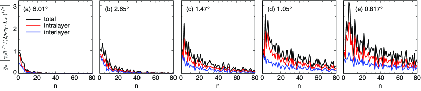
Figure 4: Plots of $\bar{g}_{n}$ as a function of the phonon band index $n$ in different twist angles. Red and blue curves are the intralayer [Eq. (62)] and interlayer [Eq. (58)] contributions, respectively, and the black curve is the total amplitude.

In the following, we numerically calculate the electron-phonon coupling for the lowest bands in TBG. The eigenstates of TBG is written as

$$|\alpha,\mathbf{k}\rangle=\sum_{\mathbf{G}Xl}F_{\alpha,\mathbf{k}}(\mathbf{G},X,l)\,|\mathbf{k}+\mathbf{G},X,l\rangle,$$ (63)

where $\alpha$ is the band index and $\mathbf{k}$ is the Bloch vector in MBZ. The electron-phonon coupling is expressed in the eigenstate basis as

$$H_{\mbox{\scriptsize e-p}}=\frac{1}{\sqrt{S}}\sum_{n\alpha\alpha^{\prime}}\sum_{\mathbf{q}\mathbf{k}\mathbf{k}^{\prime}\in{\rm MBZ}}(a^{\dagger}_{n,\mathbf{q}}+a_{n,-\mathbf{q}})c^{\dagger}_{\alpha^{\prime},\mathbf{k}^{\prime}}c_{\alpha,\mathbf{k}}\,$$

$$\hskip 113.81102pt\times g_{n,\mathbf{q}}(\alpha^{\prime},\mathbf{k}^{\prime};\alpha,\mathbf{k}),$$ (64)

where $c^{\dagger}_{\alpha,\mathbf{k}}$ and $c_{\alpha,\mathbf{k}}$ are creation and annihilation operators, respectively, of an electron in the state $|\alpha,\mathbf{k}\rangle$, and we defined

$$g_{n,\mathbf{q}}(\alpha^{\prime},\mathbf{k}^{\prime};\alpha,\mathbf{k})=$$

$$\hskip 28.45274pt\sum_{\mathbf{G}Xl}\sum_{\mathbf{G}^{\prime}X^{\prime}l^{\prime}}g_{n,\mathbf{q}}(\mathbf{k}^{\prime}+\mathbf{G}^{\prime},X^{\prime},l;\mathbf{k}+\mathbf{G},X,l)$$

$$\hskip 71.13188pt\times F^{*}_{\alpha^{\prime},\mathbf{k}^{\prime}}(\mathbf{G}^{\prime},X^{\prime},l^{\prime})F_{\alpha,\mathbf{k}}(\mathbf{G},X,l).$$ (65)

The coupling strength $g_{n,\mathbf{q}}(\alpha^{\prime},\mathbf{k}^{\prime};\alpha,\mathbf{k})$ becomes non-zero only when $\mathbf{k}^{\prime}=\mathbf{k}+\mathbf{q}+\mathbf{G}$ with moiré lattice vector $\mathbf{G}$.

To characterize the electron-phonon coupling strength in the low-lying bands, we define the averaged coupling amplitude $\bar{g}_{n}$ as

$$\bar{g}_{n}^{2}\equiv\frac{1}{N_{\mathbf{q}}}\sum_{\mathbf{q}\in{\rm MBZ}}\frac{1}{4}\sum_{\alpha=\pm}\sum_{\alpha^{\prime}=\pm}|g_{n,\mathbf{q}}(\alpha^{\prime},\bar{\mathbf{K}}+\mathbf{q};\alpha,\bar{\mathbf{K}})|^{2},$$ (66)

where $\bar{\mathbf{K}}$ is the position of the moiré Brillouin zone corner $\bar{K}$, $N_{\mathbf{q}}$ is the number of sampling points of $\mathbf{q}$ in the MBZ, which is taken as 27 in this work. The band indexes $\alpha=\pm$ represent the lowest electron band and hole band, respectively, in a single valley and spin sector, which correspond to the nearly-flat bands at the magic angle TBG. The factor $1/4$ averages the four different processes from $\alpha=\pm$ to $\alpha^{\prime}=\pm$. Here we take $\bar{\mathbf{K}}$ as the reference point, while the quantitative behavior does not depend on its choice.

Figure 4 presents the plots of $\bar{g}_{n}$ as a function of the phonon band index $n$ calculated for different twist angles. The red and blue curves are the intralayer [Eq. (62)] and interlayer [Eq. (58)] contributions, respectively, and the black curve is the total amplitude. Here the unit of the vertical axis is taken as $\gamma_{0}\sqrt{\hbar/(2\rho_{r}v_{\rm ph}L_{M})}$ where $L_{M}$ is the size of the moiré unit cell and $v_{\rm ph}$ is the typical phonon velocity of monolayer graphene. We take $v_{\rm ph}=\sqrt{\mu/\rho}\approx 1.4\times 10^{4}$ m/s, which is the velocity of the transverse acoustic phonon modes.

In large twist angles ($\theta\,\lower-1.29167pt\hbox{$>$}\kern-7.5pt\lower 3.01385pt\hbox{$\sim$}\,5^{\circ}$), we see that $\bar{g}_{n}$ decays quickly in $n$. There the superlattice hybridization is week in the low-energy region, so that each of electron and phonon eigenstates is dominated by a monolayer eigenstate with a single wave component. Then the phonons of large $n$’s (mainly composed of high $q$) do not have relevant matrix elements in the low-lying electronic states (composed of low $k$’s), and this is the reason for the quick decay of $\bar{g}_{n}$. The electron-phonon coupling in this regime is approximately given by

$$g_{q}\sim\gamma_{0}\sqrt{\frac{\hbar q}{2\rho_{r}v_{\rm ph}}},$$ (67)

which is obtained by using $\omega_{n,\mathbf{q}}\sim v_{\rm ph}q$ and $\hat{W}_{\mathbf{q}+\mathbf{G}}\sim q$ in Eq. (62). In the calculation of $\bar{g}_{n}$, the wavenumber $q$ is averaged in MBZ (of the size $\sim 1/L_{M}$), so the magnitude of $\bar{g}_{n}$ is roughly given by $\gamma_{0}\sqrt{\hbar/(2\rho_{r}v_{\rm ph}L_{M})}$, which is the vertical unit in Fig. 4.

In low twist angles, on the other hand, the wave functions spread over different $\mathbf{G}$’s in the momentum space due to the moiré superlattice hybridization, and then the phonon modes in large $n$ are able to couple the low-lying electronic states. This is observed as a long tail in Fig. 4. In this regime, the typical order of magnitude of $\hat{W}_{\mathbf{q}+\mathbf{G}}$ is given by the momentum-space distribution range of the electronic states, which is of the order of

$$\Delta q\sim\frac{t_{0}}{\hbar v}.$$ (68)

The phonon frequency $\omega_{n,\mathbf{q}}$ is of the order of $v_{ph}/L_{M}$, considering the band folding of the linear phonon dispersion. Koshino and Son (2019) As a result, the characteristic magnitude of the intralayer electron-phonon coupling, Eq. (62), becomes

$$g^{\rm(intra)}_{n,\mathbf{q}}\sim\gamma_{0}\sqrt{\frac{\hbar L_{M}}{2\rho_{r}v_{\rm ph}}}\Delta q.$$ (69)

Since $L_{M}\propto\theta^{-1}$, the overall amplitude of $g^{\rm(intra)}_{n,\mathbf{q}}$ increases in decreasing the twist angle $\theta$, and this is actually observed in Fig. 4.

The magnitude of the interlayer electron-phonon coupling Eq. (58) is estimated as

$$g^{\rm(inter)}_{n,\mathbf{q}}\sim t_{0}\sqrt{\frac{\hbar L_{M}}{2\rho_{r}v_{\rm ph}}}\frac{1}{a},$$ (70)

where we noted that $\mathbf{Q}_{j}$ is of the order of $1/a$. The relative magnitude of interlayer part to the intralayer part is

$$\frac{g^{\rm(inter)}_{n,\mathbf{q}}}{g^{\rm(intra)}_{n,\mathbf{q}}}\sim\frac{t_{0}(1/a)}{\gamma_{0}\Delta q}\sim\frac{1}{\gamma_{0}}\frac{\hbar v}{a}\approx 0.8.$$ (71)

In Fig. 4, we actually see that the two components have comparable magnitudes, while the interlayer contribution is always smaller about by a factor $\sim 2$.

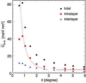
Figure 5: $\bar{U}_{\mbox{\scriptsize e-e}}$ as a functon the twist angle $\theta$. Black dots are the total amplitude, and the red squares and blue triangles are the intralayer and interlayer contributions, respectively. Dotted curve represents the low-angle expression Eq. (76) multiplied by the factor 0.6, and the dashed horizontal line indicates the exact value in the high-angle limit, 3.8 ${\rm meV\cdot nm^{2}}$.

IV.3 Phonon-mediated electron-electron interaction

The phonon-mediated electron-electron interaction is written as

$$H_{\mbox{\scriptsize e-e}}=\frac{1}{S}\sum_{\sigma\sigma^{\prime}}\sum_{\alpha\alpha^{\prime}\beta\beta^{\prime}}\sum_{\mathbf{q}\mathbf{k}\mathbf{k}^{\prime}\in{\rm MBZ}}c^{\dagger}_{\beta^{\prime}\mathbf{k}^{\prime}-\mathbf{q}\sigma^{\prime}}c^{\dagger}_{\beta\mathbf{k}+\mathbf{q}\sigma}c_{\alpha\mathbf{k}\sigma}c_{\alpha^{\prime}\mathbf{k}^{\prime}\sigma^{\prime}}$$

$$\hskip 28.45274pt\times U_{\mbox{\scriptsize e-e}}^{(\sigma,\sigma^{\prime})}(\beta^{\prime},\mathbf{k}^{\prime}-\mathbf{q};\beta,\mathbf{k}+\mathbf{q};\alpha,\mathbf{k};\alpha^{\prime},\mathbf{k}^{\prime}),$$ (72)

where $\sigma,\sigma^{\prime}$ represent the spin-valley degree of freedom which was omitted above, and we defined

$$U_{\mbox{\scriptsize e-e}}^{(\sigma,\sigma^{\prime})}(\beta^{\prime},\mathbf{k}^{\prime}-\mathbf{q};\beta,\mathbf{k}+\mathbf{q};\alpha,\mathbf{k};\alpha^{\prime},\mathbf{k}^{\prime})$$

$$=\sum_{n}g^{(\sigma)}_{n,\mathbf{q}}(\beta,\mathbf{k}+\mathbf{q};\alpha,\mathbf{k})g^{(\sigma^{\prime})}_{n,-\mathbf{q}}(\beta^{\prime},\mathbf{k}^{\prime}-\mathbf{q};\alpha^{\prime},\mathbf{k}^{\prime})\times$$

$$\frac{1}{2}\left(\frac{1}{\varepsilon_{\alpha^{\prime}\mathbf{k}^{\prime}\sigma^{\prime}}-\varepsilon_{\beta^{\prime}\mathbf{k}^{\prime}-\mathbf{q}\sigma^{\prime}}-\hbar\omega_{n,\mathbf{q}}}+\frac{1}{\varepsilon_{\beta\mathbf{k}+\mathbf{q}\sigma}-\varepsilon_{\alpha\mathbf{k}\sigma}-\hbar\omega_{n,\mathbf{q}}}\right),$$ (73)

where $\varepsilon_{\alpha\mathbf{k}\sigma}$ is the eigenenergy of state $|\alpha,\mathbf{k}\rangle$ of the spin-valley sector $\sigma$. Similar to Eq. (66), we define the averaged interaction amplitude for the lowest two bands as

$$\bar{U}_{\mbox{\scriptsize e-e}}\equiv\frac{1}{N_{\mathbf{q}}}\sum_{n,\mathbf{q}\in{\rm MBZ}}\frac{1}{4}\sum_{\alpha,\alpha^{\prime}=\pm}\frac{|g_{n,\mathbf{q}}(\alpha^{\prime},\bar{\mathbf{K}}+\mathbf{q};\alpha,\bar{\mathbf{K}})|^{2}}{-\hbar\omega_{n,\mathbf{q}}},$$ (74)

which is obviously an attractive interaction. Here we neglected $\varepsilon_{\alpha\mathbf{k}\sigma}$ in the denominator to consider the small electronic band width in the low twist angles.

We can roughly estimate the magnitude of $\bar{U}_{\mbox{\scriptsize e-e}}$ using the previous argument for the electron-phonon coupling $g_{n,\mathbf{q}}$. In the large angle regime, we replace $g_{n,\mathbf{q}}$ with Eq. (67) and $\omega_{n,\mathbf{q}}$ with $v_{\rm ph}q$, and obtain

$$\bar{U}_{\mbox{\scriptsize e-e}}\sim\frac{\gamma_{0}^{2}}{2\rho_{r}v_{\rm ph}^{2}}\sim 7.6\,{\rm meV\cdot nm^{2}}.$$ (75)

In the low angle regime, Eq. (69) and $\omega_{n,\mathbf{q}}\sim v_{ph}/L_{M}$ lead to

$$\bar{U}_{\mbox{\scriptsize e-e}}\sim\frac{\gamma_{0}^{2}}{2\rho_{r}v_{\rm ph}^{2}}(\Delta q\cdot L_{M})^{2}.$$ (76)

Here the dimensionless factor $\Delta q\cdot L_{M}$ is given by

$$\Delta q\cdot L_{M}\approx\frac{t_{0}}{\hbar v/a}\frac{1}{\theta}=\frac{2.7}{\theta{\rm[degree]}}.$$ (77)

Therefore, the electron-electron interaction amplitude is enhanced in small twist angles.

Figure 5 plots the numerically calculated $\bar{U}_{\mbox{\scriptsize e-e}}$ as a functon the twist angle $\theta$, where the black dots are the total amplitude, and the red squares and blue triangles are the intralayer and interlayer contributions, respectively. Here the dotted curve represents the low-angle expression Eq. (76) multiplied by a factor 0.6, and the dashed horizontal line indicates the exact high-angle limit, 3.8 ${\rm meV\cdot nm^{2}}$. As expected, the intralayer component rises as nearly $\propto\theta^{-2}$ in the low angle regime. The enhancement is suddenly interrupted around $0.8^{\circ}$, and it is due to the band crossing between the lowest flat bands and the excited dispersive bands. The interlayer contribution is also enhanced in the low twist angles while not as much as the intralayer part, and the total amplitude of the electron-electron interaction becomes as much as 80 ${\rm meV\cdot nm^{2}}$ at $\theta\sim 0.8^{\circ}$. The characteristic energy scale of the phonon-mediated interaction is given by $\bar{U}_{\mbox{\scriptsize e-e}}/S_{M}$ where $S_{M}=(\sqrt{3}/2)L_{M}^{2}$ is the moiré unit area. At the magic angle $\theta\sim 1^{\circ}$, in particular, $\bar{U}_{\mbox{\scriptsize e-e}}/S_{M}$ is about 0.4 meV. The dimensionless parameter for the interaction then becomes $\bar{U}_{\mbox{\scriptsize e-e}}D\sim O(1)$, where $D$ is the density of states of the flat band which is typically a few $(S_{M}\cdot{\rm meV})^{-1}$. Koshino et al. (2018) This indicates that the phonon-mediated interaction is strong in the nearly flat band.

V Conclusion

We constructed a theoretical framework to model the TBGs with lattice deformation and the electron-phonon coupling. Starting from the tight-binding model, we write down the interlayer matrix element as a function of arbitrary lattice displacement [Eq. (10)], and then obtain its long-wavelength continuum expression [Eq. (22)]. The general formula Eq. (10) works for any twist angles with arbitrary displacement vectors, and a similar theoretical treatment would be applicable to any two dimensional interfaces of van der Waals materials. The long-range version, Eq. (22), has a simpler form and it is useful to describe the low-angle TBGs with smooth lattice deformation. We actually demonstrated that the lattice relaxation effect can be implemented into the Hamiltonian by using Eq. (22), and the obtained model precisely reproduces the band structure of the original tight-binding model. Finally, we applied Eq. (22) to the phonon problem, and derived the matrix element between the electrons and moiré acoustic phonons. Finally, we numerically estimated the electron-phonon coupling and phonon mediated electron-electron interaction for the low-energy electronic states, and found a significant enhancement in the low twist angles due to the superlattice hybridization. While we focused on the long-range acoustic phonons, the electron-phonon coupling for the short wavelength vibrations (such as the optical phonons) can be described by starting from the general formula of Eq. (10). We leave the detailed studies of these problems for future work.

VI Acknowledgments

M. K. thanks the fruitful discussions with Debanjan Chowdhury. M. K. acknowledges the financial support of JSPS KAKENHI Grant Number JP17K05496.

References

- Lopes dos Santos et al. (2007) JMB Lopes dos Santos, NMR Peres, and AH Castro Neto, “Graphene bilayer with a twist: Electronic structure,” Phys. Rev. Lett. 99, 256802 (2007).
- Mele (2010) E.J. Mele, “Commensuration and interlayer coherence in twisted bilayer graphene,” Phys. Rev. B 81, 161405 (2010).
- Trambly de Laissardière et al. (2010) G. Trambly de Laissardière, D. Mayou, and L. Magaud, “Localization of dirac electrons in rotated graphene bilayers,” Nano Lett. 10, 804–808 (2010).
- Shallcross et al. (2010) S. Shallcross, S. Sharma, E. Kandelaki, and OA Pankratov, “Electronic structure of turbostratic graphene,” Phys. Rev. B 81, 165105 (2010).
- Morell et al. (2010) E.S. Morell, JD Correa, P. Vargas, M. Pacheco, and Z. Barticevic, “Flat bands in slightly twisted bilayer graphene: Tight-binding calculations,” Phys. Rev. B 82, 121407 (2010).
- Bistritzer and MacDonald (2011) R. Bistritzer and A.H. MacDonald, “Moiré bands in twisted double-layer graphene,” Proc. Natl. Acad. Sci. 108, 12233 (2011).
- Kindermann and First (2011) M. Kindermann and PN First, “Local sublattice-symmetry breaking in rotationally faulted multilayer graphene,” Phys. Rev. B 83, 045425 (2011).
- Xian et al. (2011) L. Xian, S. Barraza-Lopez, and MY Chou, “Effects of electrostatic fields and charge doping on the linear bands in twisted graphene bilayers,” Phys. Rev. B 84, 075425 (2011).
- Lopes dos Santos et al. (2012) J. M. B. Lopes dos Santos, N. M. R. Peres, and A. H. Castro Neto, “Continuum model of the twisted graphene bilayer,” Phys. Rev. B 86, 155449 (2012).
- Moon and Koshino (2012) Pilkyung Moon and Mikito Koshino, “Energy spectrum and quantum hall effect in twisted bilayer graphene,” Phys. Rev. B 85, 195458 (2012).
- de Laissardiere et al. (2012) G Trambly de Laissardiere, D Mayou, and L Magaud, “Numerical studies of confined states in rotated bilayers of graphene,” Phys. Rev. B 86, 125413 (2012).
- Popov et al. (2011) Andrey M Popov, Irina V Lebedeva, Andrey A Knizhnik, Yurii E Lozovik, and Boris V Potapkin, “Commensurate-incommensurate phase transition in bilayer graphene,” Phys. Rev. B 84, 045404 (2011).
- Brown et al. (2012) Lola Brown, Robert Hovden, Pinshane Huang, Michal Wojcik, David A Muller, and Jiwoong Park, “Twinning and twisting of tri-and bilayer graphene,” Nano Lett. 12, 1609–1615 (2012).
- Lin et al. (2013) Junhao Lin, Wenjing Fang, Wu Zhou, Andrew R Lupini, Juan Carlos Idrobo, Jing Kong, Stephen J Pennycook, and Sokrates T Pantelides, “AC/AB stacking boundaries in bilayer graphene,” Nano Lett. 13, 3262–3268 (2013).
- Alden et al. (2013) Jonathan S. Alden, Adam W. Tsen, Pinshane Y. Huang, Robert Hovden, Lola Brown, Jiwoong Park, David A. Muller, and Paul L. McEuen, “Strain solitons and topological defects in bilayer graphene,” Proc. Natl. Acad. Sci. USA 110, 11256–11260 (2013).
- Uchida et al. (2014) Kazuyuki Uchida, Shinnosuke Furuya, Jun-Ichi Iwata, and Atsushi Oshiyama, “Atomic corrugation and electron localization due to moiré patterns in twisted bilayer graphenes,” Phys. Rev. B 90, 155451 (2014).
- van Wijk et al. (2015) MM van Wijk, A Schuring, MI Katsnelson, and A Fasolino, “Relaxation of moiré patterns for slightly misaligned identical lattices: graphene on graphite,” 2D Mater. 2, 034010 (2015).
- Dai et al. (2016) Shuyang Dai, Yang Xiang, and David J Srolovitz, “Twisted bilayer graphene: Moiré with a twist,” Nano Lett. 16, 5923–5927 (2016).
- Jain et al. (2016) Sandeep K Jain, Vladimir Juričić, and Gerard T Barkema, “Structure of twisted and buckled bilayer graphene,” 2D Mater. 4, 015018 (2016).
- Nam and Koshino (2017) Nguyen N. T. Nam and Mikito Koshino, “Lattice relaxation and energy band modulation in twisted bilayer graphene,” Phys. Rev. B 96, 075311 (2017).
- Carr et al. (2018) Stephen Carr, Daniel Massatt, Steven B. Torrisi, Paul Cazeaux, Mitchell Luskin, and Efthimios Kaxiras, “Relaxation and domain formation in incommensurate two-dimensional heterostructures,” Phys. Rev. B 98, 224102 (2018).
- Lin et al. (2018) Xianqing Lin, Dan Liu, and David Tománek, “Shear instability in twisted bilayer graphene,” Phys. Rev. B 98, 195432 (2018).
- Yoo et al. (2019) Hyobin Yoo, Rebecca Engelke, Stephen Carr, Shiang Fang, Kuan Zhang, Paul Cazeaux, Suk Hyun Sung, Robert Hovden, Adam W Tsen, Takashi Taniguchi, Gyu-Chul Watanabe, Kenji Yi, Miyoung Kim, Luskin Mitchell, Ellad B. Tadmor, Efthimios Kaxiras, and Philip Kim, “Atomic and electronic reconstruction at the van der waals interface in twisted bilayer graphene,” Nat. Mater. 18, 448 (2019).
- Guinea and Walet (2019) Francisco Guinea and Niels R Walet, “Continuum models for twisted bilayer graphene: Effect of lattice deformation and hopping parameters,” Phys. Rev. B 99, 205134 (2019).
- Koshino et al. (2018) Mikito Koshino, Noah FQ Yuan, Takashi Koretsune, Masayuki Ochi, Kazuhiko Kuroki, and Liang Fu, “Maximally localized wannier orbitals and the extended hubbard model for twisted bilayer graphene,” Phys. Rev. X 8, 031087 (2018).
- Lucignano et al. (2019) Procolo Lucignano, Dario Alfè, Vittorio Cataudella, Domenico Ninno, and Giovanni Cantele, “Crucial role of atomic corrugation on the flat bands and energy gaps of twisted bilayer graphene at the magic angle ,” Phys. Rev. B 99, 195419 (2019).
- Jiang et al. (2012) Jin-Wu Jiang, Bing-Shen Wang, and Timon Rabczuk, “Acoustic and breathing phonon modes in bilayer graphene with moiré patterns,” Appl. Phys. Lett. 101, 023113 (2012).
- Cocemasov et al. (2013) Alexandr I Cocemasov, Denis L Nika, and Alexander A Balandin, “Phonons in twisted bilayer graphene,” Phys. Rev. B 88, 035428 (2013).
- Ray et al. (2016) N Ray, M Fleischmann, D Weckbecker, S Sharma, O Pankratov, and S Shallcross, “Electron-phonon scattering and in-plane electric conductivity in twisted bilayer graphene,” Phys. Rev. B 94, 245403 (2016).
- Choi and Choi (2018) Young Woo Choi and Hyoung Joon Choi, “Strong electron-phonon coupling, electron-hole asymmetry, and nonadiabaticity in magic-angle twisted bilayer graphene,” Phys. Rev. B 98, 241412 (2018).
- Angeli et al. (2019) M Angeli, E Tosatti, and M Fabrizio, “Valley jahn-teller effect in twisted bilayer graphene,” arXiv preprint arXiv:1904.06301 (2019).
- Koshino and Son (2019) Mikito Koshino and Young-Woo Son, “Moiré phonons in twisted bilayer graphene,” Phys. Rev. B 100, 075416 (2019).
- Cao et al. (2018a) Yuan Cao, Valla Fatemi, Shiang Fang, Kenji Watanabe, Takashi Taniguchi, Efthimios Kaxiras, and Pablo Jarillo-Herrero, “Unconventional superconductivity in magic-angle graphene superlattices,” Nature 556, 43 (2018a).
- Cao et al. (2018b) Yuan Cao, Valla Fatemi, Ahmet Demir, Shiang Fang, Spencer L. Tomarken, Jason Y. Luo, Javier D. Sanchez-Yamagishi, Kenji Watanabe, Takashi Taniguchi, Efthimios Kaxiras, Ray C. Ashoori, and Pablo Jarillo-Herrero, “Correlated insulator behaviour at half-filling in magic-angle graphene superlattices,” Nature 556, 80 (2018b).
- Yankowitz et al. (2019) Matthew Yankowitz, Shaowen Chen, Hryhoriy Polshyn, Yuxuan Zhang, K Watanabe, T Taniguchi, David Graf, Andrea F Young, and Cory R Dean, “Tuning superconductivity in twisted bilayer graphene,” Science 363, 1059–1064 (2019).
- Wu et al. (2018) Fengcheng Wu, AH MacDonald, and Ivar Martin, “Theory of phonon-mediated superconductivity in twisted bilayer graphene,” Phys. Rev. Lett. 121, 257001 (2018).
- Wu et al. (2019) Fengcheng Wu, Euyheon Hwang, and Sankar Das Sarma, “Phonon-induced giant linear-in- resistivity in magic angle twisted bilayer graphene: Ordinary strangeness and exotic superconductivity,” Phys. Rev. B 99, 165112 (2019).
- Lian et al. (2019) Biao Lian, Zhijun Wang, and B Andrei Bernevig, “Twisted bilayer graphene: a phonon-driven superconductor,” Phys. Rev. Lett. 122, 257002 (2019).
- Moon and Koshino (2013) Pilkyung Moon and Mikito Koshino, “Optical absorption in twisted bilayer graphene,” Phys. Rev. B 87, 205404 (2013).
- Koshino (2015) Mikito Koshino, “Interlayer interaction in general incommensurate atomic layers,” New J. Phys. 17, 015014 (2015).
- Koshino and Moon (2015) Mikito Koshino and Pilkyung Moon, “Electronic properties of incommensurate atomic layers,” J. Phys. Soc. Jpn. 84, 121001 (2015).
- Weckbecker et al. (2016) D. Weckbecker, S. Shallcross, M. Fleischmann, N. Ray, S. Sharma, and O. Pankratov, “Low-energy theory for the graphene twist bilayer,” Phys. Rev. B 93, 035452 (2016).
- Carr et al. (2019) Stephen Carr, Shiang Fang, Ziyan Zhu, and Efthimios Kaxiras, “Exact continuum model for low-energy electronic states of twisted bilayer graphene,” Phys. Rev. Research 1, 013001 (2019).
- Fang et al. (2019) Shiang Fang, Stephen Carr, Ziyan Zhu, Daniel Massatt, and Efthimios Kaxiras, “Angle-dependent Ab initio low-energy hamiltonians for a relaxed twisted bilayer graphene heterostructure,” arXiv preprint arXiv:1908.00058 (2019).
- Fleischmann et al. (2019) Maximilian Fleischmann, Reena Gupta, Florian Wullschläger, Dominik Weckbecker, Velimir Meded, Sangeeta Sharma, Bernd Meyer, and Sam Shallcross, “Perfect and controllable nesting in the small angle twist bilayer graphene,” arXiv preprint arXiv:1908.08318 (2019).
- Balents (2019) Leon Balents, “General continuum model for twisted bilayer graphene and arbitrary smooth deformations,” arXiv preprint arXiv:1909.01545 (2019).
- Ochoa (2019) Héctor Ochoa, “Moiré-pattern fluctuations and electron-phason coupling in twisted bilayer graphene,” Phys. Rev. B 100, 155426 (2019).
- Suzuura and Ando (2002) Hidekatsu Suzuura and Tsuneya Ando, “Phonons and electron-phonon scattering in carbon nanotubes,” Phys. Rev. B 65, 235412 (2002).
- Pereira and Neto (2009) Vitor M Pereira and AH Castro Neto, “Strain engineering of graphene’s electronic structure,” Phys. Rev. Lett. 103, 046801 (2009).
- Guinea et al. (2010) F Guinea, MI Katsnelson, and AK Geim, “Energy gaps and a zero-field quantum hall effect in graphene by strain engineering,” Nat. Phys. 6, 30–33 (2010).
- Tarnopolsky et al. (2019) Grigory Tarnopolsky, Alex Jura Kruchkov, and Ashvin Vishwanath, “Origin of magic angles in twisted bilayer graphene,” Phys. Rev. Lett. 122, 106405 (2019).
- Liu et al. (2019) Jianpeng Liu, Junwei Liu, and Xi Dai, “Pseudo landau level representation of twisted bilayer graphene: Band topology and implications on the correlated insulating phase,” Phys. Rev. B 99, 155415 (2019).
- San-Jose et al. (2014) Pablo San-Jose, A Gutiérrez-Rubio, Mauricio Sturla, and Francisco Guinea, “Electronic structure of spontaneously strained graphene on hexagonal boron nitride,” Phys. Rev. B 90, 115152 (2014).
- Zakharchenko et al. (2009) KV Zakharchenko, MI Katsnelson, and Annalisa Fasolino, “Finite temperature lattice properties of graphene beyond the quasiharmonic approximation,” Phys. Rev. Lett. 102, 046808 (2009).
- Jung et al. (2015) Jeil Jung, Ashley M DaSilva, Allan H MacDonald, and Shaffique Adam, “Origin of band gaps in graphene on hexagonal boron nitride,” Nat. Commun. 6, 6308 (2015).
- Lebedeva et al. (2011) Irina V Lebedeva, Andrey A Knizhnik, Andrey M Popov, Yurii E Lozovik, and Boris V Potapkin, “Interlayer interaction and relative vibrations of bilayer graphene,” Phys. Chem. Chem. Phys. 13, 5687–5695 (2011).