Interplay of dipoles and spins in $\kappa$-(BEDT-TTF)${}_{2}X$, where $X=$ Hg(SCN)₂Cl, Hg(SCN)₂Br, Cu[N(CN)₂]Cl, Cu[N(CN)₂]Br, and Ag₂(CN)₃

Abstract

We combine first principles density functional calculations with empirical relationships for the Coulomb interactions in the ‘monomer’ model of $\kappa$-(BEDT-TTF)${}_{2}X$. This enables us to calculate the parameters for the model of coupled dipolar and spin degrees of freedom proposed by Hotta [Phys. Rev. B 82, 241104 (2010)], and Naka and Ishihara [J. Phys. Soc. Japan 79, 063707 (2010)]. In all materials studied, retaining only the largest interactions leads to a transverse field Ising model of the dipoles. This quantifies, justifies and confirms recent claims that the dipoles are of crucial importance for understanding these materials. We show that two effects are responsible for a range of behaviors found in the dipoles in different $\kappa$-(BEDT-TTF)${}_{2}X$ salts. (i) The inter-dimer hopping, $t_{b1}$, which gives rise to the “transverse field” in the Ising model for the dipoles ($H^{T}=2t_{b1}$), is between a third and a tenth smaller in the mercuric materials than for the mercury-free salts. (ii) The Ising model of dipoles is in the quasi-one-dimensional limit for the mercuric salts, but quasi-two-dimensional (between the square and isotropic triangular limits) for the mercury-free materials. Thus, the dimensionless critical field is much smaller in the mercuric compounds. Effect (ii) is much larger than effect (i). Simple explanations of both effects based on the band structures of the different salts are given. We show that dipolar order and even short-range dipolar correlations have a profound impact on the nature of the interdimer magnetic (superexchange) interactions. For example, dipole crystallization drives the materials towards quasi-one-dimensional magnetic interactions, which could be important for understanding the spin liquids found in some of these materials.

I Introduction

Which, if any, symmetries are spontaneously broken in the dimer Mott insulating phase of the $\kappa$-(BEDT-TTF)${}_{2}X$ depends crucially on the anion, $X$. $\kappa$-(BEDT-TTF)₂Cu[N(CN)₂]Cl (henceforth $\kappa$-CuCl) and $\kappa$-(BEDT-TTF)₂Cu[N(CN)₂]Br (henceforth $\kappa$-CuBr) show antiferromagnetic order, but no long-range magnetic order is observed in $\kappa$-(BEDT-TTF)₂Cu₂(CN)₃ (henceforth $\kappa$-CuCN) or $\kappa$-(BEDT-TTF)₂Ag₂(CN)₃ (henceforth $\kappa$-AgCN) down to the lowest temperatures that have been investigated. The standard model of these materials Kino and Fukuyama (1996); McKenzie (1998); Powell and McKenzie (2006) begins from an (extended) Hubbard model with one orbital per BEDT-TTF, Fig. 1a. This model is three quarters filled because the anion removes one electron per formula unit from the organic layer. However, as these salts are strongly dimerized, it is often assumed that the interdimer bonding and antibonding orbitals are energetically well separated. This assumption suggests that one can neglect the fully occupied bonding orbitals, leaving a half-filled Hubbard model with one orbital per dimer (BEDT-TTF)₂, Fig. 1b,c.

In the Mott insulating phase of the dimer model, charge fluctuations can be integrated out to leave a Heisenberg model on the anisotropic triangular lattice Fig. 1c McKenzie (1998); Powell and McKenzie (2011). This model is of intrinsic theoretical interest and it extrapolates between the square lattice ($J_{1}=0$), the triangular lattice ($J_{1}=J_{2}$) and one-dimensional chains with a frustrated interchain coupling ($J_{2}\rightarrow 0$).

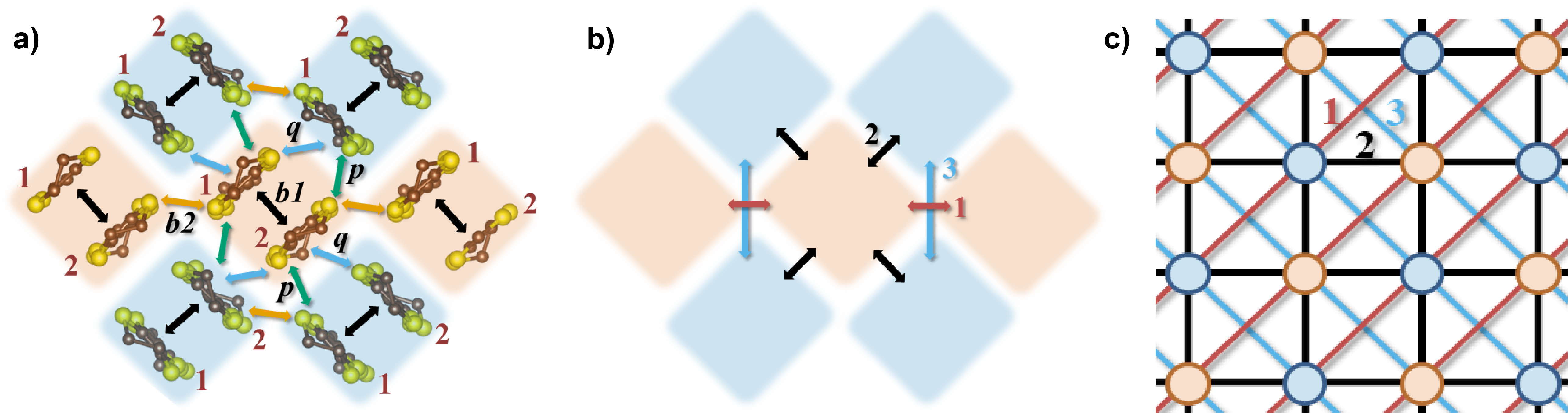
Figure 1: Structure of models of $\kappa$-(BEDT-TTF)${}_{2}X$. a) A single layer of $\kappa$-(BEDT-TTF)${}_{2}X$ (hydrogen atoms and counter-ions are not shown). The various inter-molecular hopping integrals, i.e., $t_{\mu\nu ij}$ are labeled according to the standard monomer convention and, for simplicity, only the subcripts $\mu\nu ij\in\{b1,b2,p,q\}$ are shown. The two sublattices of ET dimers are highlighted in peach and blue. b) The dimer model. Here the subscripts 1, 2, or 3 will be used label various interactions, e.g., hopping $t$, exchange $J$, dipole-dipole coupling $K$, or Dzyaloshinskii-Moriya coupling $\bm{D}$. c) This model is topologically equivalent to a square lattice with different couplings across the two diagonals or, if the ‘3’ interactions are negligible, an anisotropic triangular lattice.

However, the validity of the dimer model has been questioned. Several groups have argued theoretically that the charge degrees of freedom within the dimer cannot be neglected and may be responsible for some of the most interesting behavior observed in $\kappa$-(BEDT-TTF)${}_{2}X$, including the spin-liquid behavior and superconductivity Clay and Mazumdar (2019); Hotta (2010); Naka and Ishihara (2010). Experimental support for these ideas has come from the observation of ferroelectricity arising from electronic dipoles associated with charge order within the dimers that spontaneously break inversion symmetry in several $\kappa$-(BEDT-TTF)${}_{2}X$ salts Lunkenheimer et al. (2012); Iguchi et al. (2013); Abdel-Jawad et al. (2010).

Recently, the $\kappa$-(BEDT-TTF)₂Hg(SCN)${}_{2}Y$ salts have emerged as an important testing ground for the interplay between dipole and spin order. Long-range dipole order has been obeserved in $\kappa$-(BEDT-TTF)₂Hg(SCN)₂Cl (henceforth $\kappa$-HgCl) Drichko et al. (2014); Gati et al. (2018) and, collectively, several experiments suggest that a dipole liquid has been seen in $\kappa$-(BEDT-TTF)₂Hg(SCN)₂Br (henceforth $\kappa$-HgBr) Hassan et al. (2018). Interestingly, it has been suggested that these materials may be an intermediate class with weaker dimerization than other $\kappa$-phase salts Drichko et al. (2014); Gati et al. (2018), but stronger dimerization than, say, the $\theta$ phase BEDT-TTF salts Seo et al. (2004).

One approach to understanding the interaction between spin and charge order in the $\kappa$-(BEDT-TTF)${}_{2}X$ salts is to study the monomer model (Fig. 1) Clay and Mazumdar (2019). But an alternative, physically appealing, approach has been introduced by Hotta Hotta (2010) and, independently, Naka and Ishihara Naka and Ishihara (2010) (HIN). They introduce a binary variable, which describes the dipole or charge degree of freedom within the dimer. HIN showed that this leads to a transverse field Ising model (TFIM) for the dipoles, a Heisenberg model for the spin on the dimers, and coupling terms between the spin and dipole degrees of freedom, reminiscent of the Kugel-Khomskii interaction between spins and orbital degrees of freedom Pavarini (2016).

In this paper we derive a first principles tight-binding monomer model for $\kappa$-HgCl, $\kappa$-HgBr, $\kappa$-CuCl, $\kappa$-CuBr, and $\kappa$-AgCN. We use this model, and empirical relationships for the effective Coulomb interactions, to parameterise an extended HIN model for these materials. We find that, in all materials, the coupling constants for the TFIM of the dipoles are the largest energy scales in the problem.

The TFIM has been extensively studied in each of the limits of the lattice dimer model, Fig. 1. In one dimension, the dimensionless critical field is $h_{c}\equiv H^{T}_{c}/K_{\text{max}}=1$, where $H^{T}_{c}$ is the critical transverse field and $K_{\text{max}}$ is the (largest) Ising coupling constant. On the isotropic triangular lattice $h_{c}=4.768$ Blöte and Deng (2002) and on the square lattice $h_{c}=3.044$ du Croo de Jongh and van Leeuwen (1998); Blöte and Deng (2002). However, we are not aware of any studies on the anisotropic triangular lattice, Fig. 1c, beyond these limits. In the TFIM description of the dipoles in $\kappa$-(BEDT-TTF)${}_{2}X$, there is a direct proportionality between the transverse field and the intradimer hopping ($H^{T}\propto t_{b1}$). There is ferroelectric order in the low field regime and quantum disorder in the high field regime.

We show that two effects are responsible for different ferroelectric behaviors of the $\kappa$-(BEDT-TTF)${}_{2}X$ salts. (i) The inter-dimer hopping, $t_{b1}$, which gives rise to the “transverse field” in the Ising model for the dipoles ($H=2t_{b1}$), is between a third and a tenth smaller in $\kappa$-HgCl and $\kappa$-HgBr than in $\kappa$-CuCl, $\kappa$-CuBr, and $\kappa$-AgCN. (ii) The TFIM of dipoles is in the quasi-one-dimensional limit for $\kappa$-HgCl and $\kappa$-HgBr, but quasi-two-dimensional (between the square and isotropic triangular limits) for $\kappa$-CuCl, $\kappa$-CuBr, and $\kappa$-AgCN. Thus, the dimensionless critical field is much smaller in the former pair of compounds. We discuss the implications of this for the magnetic behaviors of these salts.

II Density functional calculations

We computed the electronic structures of $\kappa$-HgCl, $\kappa$-HgBr, $\kappa$-CuCl, $\kappa$-CuBr, and $\kappa$-AgCN from four-component relativistic density functional theory with the FPLO package in an all-electron full-potential local orbital basis Eschrig et al. (2004); Koepernik and Eschrig (1999). For $\kappa$-CuBr we consider fully dueterated BEDT-TTF molecules (as this drives this salt insulating Taniguchi et al. (1999)), for all other anions we consider fully protonated BEDT-TTF. The density was converged on a $(8\times 8\times 8)$ $k$ mesh using the Perdew, Burke and Ernzerhof (PBE) generalized gradient approximation Perdew et al. (1996). We produced localised Wannier spin-orbitals for the frontier bands (those closest to the Fermi energy), and from those produced an ab initio single electron Hamiltonian containing one Wannier orbital, $|\mu i\alpha\rangle$, per spin species, $\alpha$, on every BEDT-TTF molecule, $i$ in every dimer, $\mu$. The geometries were taken from the measured crystal structures Drichko et al. (2014); Schlueter (2018); Geiser et al. (1991a, b); Saito (2015) as indicated in Table 1.

The complex overlaps between the Wannier spin-orbitals,

$$h_{\mu\nu ij\alpha\beta}=\langle\mu i\alpha|\hat{\mathcal{H}}|\nu j\beta\rangle,$$ (1)

where $\hat{\mathcal{H}}$ is the full microscopic Hamiltonian, lead to a spin-dependent model Hamiltonian:

$$\hat{H}=\sum_{\mu,\nu}\sum_{i,j}\sum_{\alpha,\beta}\hat{c}^{\dagger}_{\mu i\alpha}h_{\mu\nu ij\alpha\beta}\hat{c}_{\nu j\beta},$$ (2)

where $\hat{c}^{(\dagger)}_{\mu i\alpha}$ annihilates (creates) an electron in the spin $\alpha$ Wannier centered on the $i$th molecule of the $\mu$th dimer. The SU(2) symmetry of the Hamiltonian implies that $h_{\mu\nu ij}=t_{\mu\nu ij}I_{2}+\bm{\lambda}_{\mu\nu ij}\cdot\bm{\sigma}$, where $I_{2}$ is the identity matrix and $\bm{\sigma}$ is the vector of Pauli matrices. Thus,

$$\hat{H}=\sum_{\mu,\nu}\sum_{i,j}\sum_{\alpha,\beta}\hat{c}^{\dagger}_{\mu i\alpha}\Big{(}t_{\mu\nu ij}\delta_{\alpha\beta}+i\bm{\lambda}_{\mu\nu ij}\cdot\bm{\sigma}_{\alpha\beta}\Big{)}\hat{c}_{\nu j\beta}.$$ (3)

Physically, the scalar hopping integrals, $t_{\mu\nu ij}$, describe spin independent hopping between molecules and the vector hopping integrals, $\bm{\lambda}_{\mu\nu ij}$, which parameterize the spin-orbit coupling, allow for both spin dependent hopping ($\lambda^{z}_{\mu\nu ij}$) and hopping with a spin flip ($\lambda^{x}_{\mu\nu ij}$, $\lambda^{y}_{\mu\nu ij}$).

A typical band structure is shown in Fig. 2. We display three different approximations to the electronic structure: (i) the band structure directly calculated from four component DFT; (ii) the band structure calculated from the full set of overlaps between Wannier orbitals, $\{h_{\mu\nu ij\alpha\beta}\}$; and (iii) the standard monomer model, Fig. 1a, which contains only the largest overlaps of our ab initio model Hamiltonian. As expected in both materials the full Wannier band structure reproduces the direct DFT results exactly, consistent with a successful Wannier orbital construction. The monomer model clearly captures the key features of the electronic structure and gives a clearer picture of the physical mechanisms at play than the full DFT calculation. Therefore, we will use this model as the basis for analysis of these materials. Also, note the Dirac points at $Y$ in $\kappa$-HgCl and $\kappa$-HgBr (not shown).

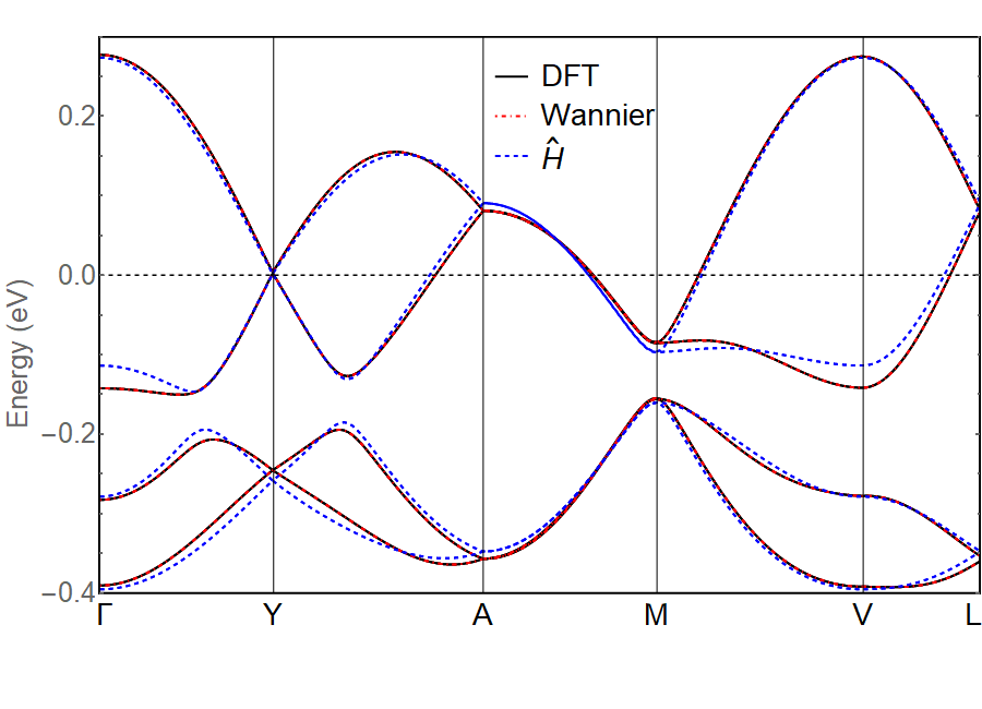
Figure 2: The calculated band structure of $\kappa$-HgCl. The direct density functional calculations (solid black line) is exactly reproduced by the Wannier model Hamiltonian (dot-dashed red line). The monomer model [$\hat{H}$, blue dashed line, Fig. 1, Eq. (3)], which retains only the four largest hopping integrals, captures the main features of the band structure.

The monomer model is based on Eq. (3) but restricted to contain only the largest parameters ($t_{\mu\nu ij}$ and $\bm{\lambda}_{\mu\nu ij}$). As in other $\kappa$-phase BEDT-TTF salts, there are four large interactions in both of the $\kappa$-(BEDT-TTF)₂Hg(SCN)${}_{2}Y$ salts. We use the standard bond-labeling convention, illustrated in Fig. 1a. The parameters for this model are reported in Table 1. The scalar hopping integrals for these salts are in excellent agreement with a previous scalar relativistic and non-relativistic calculations where these have previously been reported Gati et al. (2018); Koretsune and Hotta (2014).

	$t_{b1}$	$t_{b2}$	$t_{p}$	$t_{q}$	$\sqrt{t_{p}^{2}-t_{q}^{2}}$	${\bm{\lambda}}_{p}$	${\bm{\lambda}}_{q}$	$\bm{r}_{p}$	$\bm{r}_{q}$
$\kappa$-HgCl Drichko et al. (2014)	120	88	63	34	33	$(0.83,-0.07,0.32)$	$(0.37,-0.13,0.08)$	$(0.00,-2.72,11.09)$	$(3.60,-7.67,-7.59)$
$\kappa$-HgBr Schlueter (2018)	126	83	60	40	45	$(0.40,0.06,0)$	$(1.47,0.10,-0.53)$	$(0.00,-2.76,11.01)$	$(3.47,-7.75,7.51)$
$\kappa$-CuCl Geiser et al. (1991a)	142	60	90	44	79	$(-0.54,-0.91,0)$	$(0.37,-0.68,0)$	$(7.61,-0.99,7.95)$	$(-12.12,0.00,3.47)$
$\kappa$-CuBr Geiser et al. (1991b)	178	61	98	37	91	$(-0.46,-0.87,0)$	$(0.30,-0.84,0)$	$(7.58,-0.99,8.00)$	$(-12.16,0.00,3.53)$
$\kappa$-AgCN Saito (2015)	180	66	87	19	85	$(-0.55,-0.01,0.98)$	$(-0.03,-0.29,-0.07)$	$(-1.03,8.16,-7.84)$	$(0.00,3.70,12.43)$

Table 1: Calculated intra-layer scalar ($t$) and vector ($\bm{\lambda}$) hopping integrals in meV and the relevant vectors in Å. ${\bm{\lambda}}_{b1}={\bm{\lambda}}_{b2}=\bm{0}$ in all materials due to inversion symmetries. $\bm{r}_{p}$ and $\bm{r}_{q}$ define the direction of the vector hopping [reversing the direction changes the sign – as required for the hermiticity of Eq. (3)]. $\sqrt{t_{p}^{2}-t_{q}^{2}}$ is included here as, we will see below, it is a crucial parameter for understanding the behavior of these materials. Note that it is much smaller in $\kappa$-HgCl and $\kappa$-HgBr than in the other materials.

III Coupled spin and dipole order

In this section we generalize the model of interacting dipoles and spins introduced by Hotta, Naka and Ishihara Naka and Ishihara (2010); Hotta (2010) and use our density functional theory results as the basis for a calculation of the parameters of the model. The derivation assumes that these materials are in the strong coupling limit where the electron-electron interactions within the dimer are large, and all other terms can be treated perturbatively. The unperturbed model is

$$\hat{H}^{(0)} = \sum_{\mu}\Bigg{[}U\sum_{i}\hat{n}_{\mu i\uparrow}\hat{n}_{\mu i\downarrow}+\left(V_{b1}-\frac{J_{b1}}{2}\right)\hat{n}_{\mu 1}\hat{n}_{\mu 2}$$ (4)

$$+J_{b1}\left(\hat{c}_{\mu 1\uparrow}^{\dagger}\hat{c}_{\mu 1\downarrow}^{\dagger}\hat{c}_{\mu 2\uparrow}\hat{c}_{\mu 2\downarrow}+\hat{c}_{\mu 2\uparrow}^{\dagger}\hat{c}_{\mu 2\downarrow}^{\dagger}\hat{c}_{\mu 1\uparrow}\hat{c}_{\mu 1\downarrow}\right)$$

$$-2J_{b1}\hat{\bm{S}}_{\mu 1}\cdot\hat{\bm{S}}_{\mu 2}\Bigg{]},$$

where $i=1$ and $2$ indicate the two BEDT-TTF molecules within the same dimer, $\hat{n}_{\mu i\alpha}=\hat{c}^{\dagger}_{\mu i\alpha}\hat{c}_{\mu i\alpha}$, $\hat{n}_{\mu i}=\sum_{\alpha}\hat{n}_{\mu i\alpha}$, and $\hat{\bm{S}}_{\mu i}=\frac{1}{2}\sum_{\alpha,\beta}\hat{c}^{\dagger}_{\mu i\alpha}\bm{\sigma}_{\alpha\beta}\hat{c}_{\mu i\beta}$. At three-quarters filling, relevant to $\kappa$-(BEDT-TTF)${}_{2}X$, there are four degenerate ground states: $|\uparrow\downarrow,\uparrow\rangle$, $|\uparrow\downarrow,\downarrow\rangle$, $|\uparrow,\uparrow\downarrow\rangle$, and $|\downarrow,\uparrow\downarrow\rangle$.

Intra-dimer hopping and inter-dimer interactions give rise to first order perturbations. We write their sum as

$$\hat{H}^{(1)} = t_{b1}\sum_{\mu\sigma}\hat{c}^{\dagger}_{\mu 1\sigma}\hat{c}_{\mu 2\sigma}$$

$$+\frac{1}{2}\sum_{\mu\neq\nu}\sum_{i,j}\Bigg{[}\left(V_{\mu\nu}^{ij}-\frac{J_{\mu\nu}^{ij}}{2}\right)\hat{n}_{\mu i}\hat{n}_{\nu j}$$

$$-2J_{\mu\nu}^{ij}\hat{\bm{S}}_{\mu i}\cdot\hat{\bm{S}}_{\nu j}+J_{\mu\nu}^{ij}\hat{c}_{\mu i\uparrow}^{\dagger}\hat{c}_{\mu i\downarrow}^{\dagger}\hat{c}_{\nu j\uparrow}\hat{c}_{\nu j\downarrow}\Bigg{]}.$$

Throughout we adopt the convention that within any pair of dimers the labels $i$ and $j$ are chosen so that the shortest separation connects site 1 on one dimer with site 2 on the other, this preserves translation symmetry within each sublattice, cf. Fig. 1.

Within the low-energy subspace these terms can be dramatically simplified by the introduction of two new operators: the dimer spin operator, $\hat{\bm{S}}_{\mu}=\frac{1}{2}\sum_{i,\alpha,\beta}\hat{c}^{\dagger}_{\mu i\alpha}\bm{\sigma}_{\alpha\beta}\hat{c}_{\mu i\beta}$, and the dipole operator $\hat{\bm{T}}_{\mu}=\frac{1}{2}\sum_{i,j,\alpha}\hat{c}^{\dagger}_{\mu i\alpha}\bm{\sigma}_{ij}\hat{c}_{\mu j\alpha}$. Our four degenerate ground states can be rewritten as $(S^{z},T^{z})=(\frac{1}{2},\frac{1}{2})$, $(-\frac{1}{2},\frac{1}{2})$, $(\frac{1}{2},-\frac{1}{2})$, and $(-\frac{1}{2},-\frac{1}{2})$ respectively. This allows us to write

$$\hat{H}^{(1)} = H^{T}\sum_{\mu}\hat{T}^{x}_{\mu}+\sum_{\mu\neq\nu}W^{TT}_{\mu\nu}\hat{T}^{z}_{\mu}\hat{T}^{z}_{\nu}$$ (6)

$$+\sum_{\mu\neq\nu}\left[W_{\mu\nu}^{SS}+W_{\mu\nu}^{SST}(\hat{T}^{z}_{\mu}+\hat{T}^{z}_{\nu})\right.$$

$$\left.\hskip 56.9055pt+W_{\mu\nu}^{SSTT}\hat{T}^{z}_{\mu}\hat{T}^{z}_{\nu}\right]\hat{\bm{S}}_{\mu}\cdot\hat{\bm{S}}_{\nu},$$

where $H^{T}=2t_{b1}$,

$$W^{TT}_{\mu\nu} = (V_{\mu\nu}^{11}-V_{\mu\nu}^{12}-V_{\mu\nu}^{21}+V_{\mu\nu}^{22})$$ (7)

$$-\frac{1}{2}(J_{\mu\nu}^{11}-J_{\mu\nu}^{12}-J_{\mu\nu}^{21}+J_{\mu\nu}^{22}),$$

$W_{\mu\nu}^{SS}=\frac{1}{4}(J_{\mu\nu}^{11}+J_{\mu\nu}^{12}+J_{\mu\nu}^{21}+J_{\mu\nu}^{22})$, $W_{\mu\nu}^{SST}=\frac{1}{2}(J_{\mu\nu}^{11}+J_{\mu\nu}^{12}-J_{\mu\nu}^{21}-J_{\mu\nu}^{22})$, $W_{\mu\nu}^{SSTT}=J_{\mu\nu}^{11}-J_{\mu\nu}^{12}-J_{\mu\nu}^{21}+J_{\mu\nu}^{22}$, and we have used the symmetries $V_{\mu\nu}^{ij}=V_{\nu\mu}^{ji}$, $J_{\mu\nu}^{ij}=J_{\nu\mu}^{ji}$ and the inversion symmetry of the crystals (which, although spontaneously broken in the dipoled ordered phase, is respected by the underlying Hamiltonian).

The first two terms of Eq. (6) are simply the TFIM for the dipole variables, $\hat{\bm{T}}_{\mu}$. The last two lines describe direct dimer exchange interactions ($W_{\mu\nu}^{SS}$) and three ($W_{\mu\nu}^{SST}$) and four ($W_{\mu\nu}^{SSTT}$) body interactions between the dipole Ising variables and the spins. The interdimer exchange interactions ($J_{\mu\nu}^{ij}$) are around two orders of magnitude smaller than direct interdimer Coulomb interactions ($V_{\mu\nu}^{ij}$), so the first two terms in Eq. (6) are significantly larger than others (although we see below that these terms are not negligible for describing the magnetic order). Therefore it is reasonable to start by examining only the TFIM for $\hat{T}^{x}_{\mu}$. It is also important to note that the Ising coupling constants, $W_{\mu\nu}^{TT}$, are given by a “differential” Coulomb interaction, Eq. (7).

It has been demonstrated that in full three-dimensional models of BEDT-TTF salts $V_{\mu\nu}^{ij}\propto 1/r$, to a high degree of accuracy Shinaoka et al. (2012), where $r$ is the distance between the centers of the Wannier orbitals, and $V_{b2}\sim 0.4$ in a wide range of salts Koretsune and Hotta (2014); Nakamura et al. (2009). These two relationships yield the Ising coupling constants listed in Table 2. The differences between the different materials result primarily from changes in the way the dimers are arranged within the crystal. These structural differences are much larger than changes of the intradimer separation, which only varies between 3.67 and 3.73 Å across all materials studied.

It is apparent from Eq. (7) that the $W^{TT}$ can take either sign. However, one’s physical intuition is that if the dimers are close to each other (relative to the intradimer separation) then $W^{TT}$ should be negative. This is indeed confirmed by the values in Table 2, with the only positive values being $W_{3}^{TT}$ for $\kappa$-HgCl and $\kappa$-HgBr and $W_{\perp}^{TT}$ for $\kappa$-AgCN. In each of these cases the interdimer separation is large compared to intradimer separation and the argument above becomes invalid. Given the signs in the first order Hamiltonian, Eq. (6), (positive) negative $W^{TT}$ corresponds to (anti)ferro-dipolar coupling. Nevertheless, because of the relative arrangement of the sublattices of the dimers, cf. Fig. 1a, long range (anti)ferro-dipolar order does not correspond to simple (anti)parallel arrangements of the dipoles on the two different sublattices.

$X$	$W^{TT}_{1}$	$W^{TT}_{2}$	$W^{TT}_{3}$	$W^{TT}_{\perp}$
Hg(SCN)2Cl	-8	-22	13	-3
Hg(SCN)2Br	-11	-21	13	-3
Cu[N(CN)2]Cl	-5	-54	-12	-11
Cu[N(CN)2]Br	-5	-54	-12	-11
Ag2(CN)3	-4	-53	-12	1

Table 2: Calculated Ising coupling constants at first order in the interdimer Coulomb interactions, cf. Eq. (7), for the dipole degrees of freedom. We neglect the $J_{\mu\nu}^{ij}$ as these are two orders of magnitude smaller than the $V_{\mu\nu}^{ij}$ Nakamura et al. (2012). All values in meV.

Virtual hopping between dimers induces additional interactions. Hopping within a single dimer sublattice, cf. Fig. 1, is described by

$$\hat{H}_{1}=t_{b2}\sum_{\langle\mu,\nu\rangle}\sum_{\sigma}\hat{c}^{\dagger}_{\mu 2\sigma}\hat{c}_{\nu 1\sigma}+H.c.,$$ (8)

where $\langle\mu,\nu\rangle$ indicates that the sum runs over nearest neighbors on the same sublattice only. At second order in $t_{b2}$ this induces interactions given by

$$\hat{H}^{(2)}_{1} = \sum_{\langle\mu,\nu\rangle}\Big{\{}X_{TT}\hat{T}^{z}_{\mu}\hat{T}^{z}_{\nu}+X_{T}(\hat{T}^{z}_{\mu}-\hat{T}^{z}_{\nu})$$ (9)

$$\hskip 19.91692pt+\Big{[}X_{SSTT}\hat{T}^{z}_{\mu}\hat{T}^{z}_{\nu}+X_{SST}(\hat{T}^{z}_{\mu}-\hat{T}^{z}_{\nu})$$

$$\hskip 34.1433pt+X_{SS}\Big{]}\hat{\bm{S}}_{\mu}\cdot\hat{\bm{S}}_{\nu}\Big{\}}.$$

Analytic expressions for the coupling constants are given in the Appendix.

A key observation from these analytic expressions is that $X_{TT}$ is generically positive, i.e., antiferro-dipolar. This is the opposite sign from that expected (and calculated) for $W_{1}^{TT}$, the equivalent interaction arising from the direct Coulomb interaction. However, it is the same sign as one expects from a simple superexchange interaction, $X_{SS}$, which also arises at second order in $t_{b2}^{2}/U$. The processes that give rise to this $X_{TT}$ are sketched in Fig. 3.

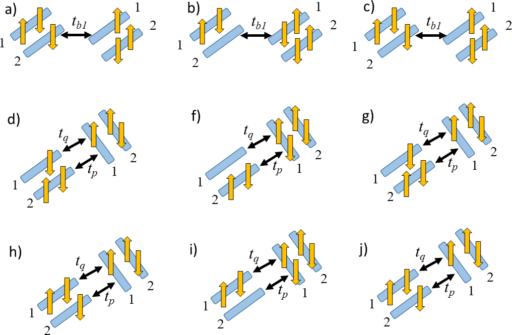
Figure 3: Sketches of prototypical second order processes leading to the Ising coupling between dipoles. Recall that second order processes always lower the energy of the ground state. Processes like $a\rightarrow b\rightarrow c$ are only available if dipoles on the two dimes are antiparallel. Thus, this leads to an antiferro-dipolar coupling ($X_{TT}<0$). Processes like $d\rightarrow e\rightarrow f$ are only allowed if dipoles on the two dimes are the same sign and therefore favor ferro-dipolar coupling ($Y_{TT}>0$). However, processes like $h\rightarrow i\rightarrow j$ are only possible if dipoles on the two dimes are antialigned and therefore favor antiferro-dipolar coupling ($Y_{TT}<0$). The competition between the processes $d\rightarrow e\rightarrow f$ and $h\rightarrow i\rightarrow j$ is vital for understanding the different dimensionalities of the TFIM in the mercuric and mercury-free salts as it means the $Y_{TT}\propto t_{p}^{2}-t_{q}^{2}$.

Hopping between different dimer sublattices is described by the terms

$$\hat{H}_{2}=\sum_{[\mu,\nu]}\sum_{\sigma}\left(t_{p}\hat{c}^{\dagger}_{\mu 2\sigma}\hat{c}_{\nu 1\sigma}+t_{q}\hat{c}^{\dagger}_{\mu 2\sigma}\hat{c}_{\nu 2\sigma}\right)+H.c.,$$ (10)

where $[\mu,\nu]$ indicates that the sum runs over nearest neighbors on the different sublattices only.

At second order in $t_{p}$ and $t_{q}$, the effective Hamiltonian is

$$\hat{H}^{(2)}_{2} = \sum_{[\mu,\nu]}\Big{\{}Y_{TT}\hat{T}^{z}_{\mu}\hat{T}^{z}_{\nu}+Y_{zx}\hat{T}^{z}_{\mu}\hat{T}^{x}_{\nu}+Y_{T-}(\hat{T}^{z}_{\mu}-\hat{T}^{z}_{\nu})+Y_{T+}(\hat{T}^{z}_{\mu}+\hat{T}^{z}_{\nu})+Y_{x}\hat{T}^{x}_{\nu}$$ (11)

$$+\Big{[}Y_{SSTT}\hat{T}^{z}_{\mu}\hat{T}^{z}_{\nu}+Y_{SSzx}\hat{T}^{z}_{\mu}\hat{T}^{x}_{\nu}+Y_{SSx}\hat{T}^{x}_{\nu}+Y_{SST-}(\hat{T}^{z}_{\mu}-\hat{T}^{z}_{\nu})+Y_{SST+}(\hat{T}^{z}_{\mu}+\hat{T}^{z}_{\nu})+Y_{SS}\Big{]}\hat{\bm{S}}_{\mu}\cdot\hat{\bm{S}}_{\nu}$$

$$+\Big{[}Y_{4Szx}\hat{T}^{z}_{\mu}\hat{T}^{x}_{\nu}+Y_{4Sx}\hat{T}^{x}_{\nu}\Big{]}\left(\hat{\bm{S}}_{\mu}\cdot\hat{\bm{S}}_{\nu}\right)^{2}\Big{\}}.$$

Again, the analytical expressions for the coupling constants are given in the Appendix.

It is interesting to note here that the values of the $Y$ parameters, most importantly $Y_{TT}\propto(t_{p}^{2}-t_{q}^{2})$ [see Eq. (31)], depend sensitively on the relative magnitudes of $t_{p}$ and $t_{q}$ (reported in Table 1). This has a simple physical origin, explained in Fig. 3. This will be crucial for understanding the different physics observed in the different materials.

To evaluate the $X$ and $Y$ parameters we take $U=V_{b1}$, $J_{b1}=V_{b1}/2.5$ Nakamura et al. (2009) and $V_{b1}$ given by the parameterization above . This yields the parameters in Table 3. Notice that the largest parameters here are an order of magnitude more than those arising from the first order corrections, Table 2. We stress that this does not indicate an issue with the convergence of the perturbative expansion, as these corrections are second order in inter-dimer hopping integrals and the parameters in Table 2 are first order in the inter-dimer Coulomb interactions.

The two largest parameters, $X_{TT}$ and $Y_{TT}$, are quite different in $\kappa$-HgCl and $\kappa$-HgBr than in the other materials. $X_{TT}\propto t_{b2}^{2}$ [see Eq. (26)] and $t_{b2}$ is 25-50% larger in $\kappa$-HgCl and $\kappa$-HgBr than the other materials, see Table 1, which means that $X_{TT}$ is much bigger in the mercuric materials. $Y_{TT}\propto(t_{p}^{2}-t_{q}^{2})$ [see Eq. (31)] and $t_{p}$ is $\sim 50\%$ larger in the mercury-free materials, which results in a much larger $Y_{TT}$ in these systems.

$X$	$X_{TT}$	$X_{T}$	$X_{SSTT}$	$X_{SST}$	$X_{SS}$	$Y_{TT}$	$Y_{zx}$	$Y_{Tm}$	$Y_{Tp}$	$Y_{x}$	$Y_{SSTT}$	$Y_{SSzx}$	$Y_{SST-}$	$Y_{SST+}$	$Y_{SSx}$	$Y_{SS}$	$Y_{4Szx}$	$Y_{4Szx}$
Hg(SCN)2Cl	288	-6	-46	-23	23	105	-40	-3	-1	-20	-17	-38	-12	-3	-19	8	26	26
Hg(SCN)2Br	254	-5	-41	-20	20	74	-44	-3	-1	-22	-12	-43	-11	-5	-21	6	28	28
Cu[N(CN)2]Cl	131	-3	-21	-11	11	225	-72	-6	-1	-36	-36	-69	-24	-6	-35	18	46	46
Cu[N(CN)2]Br	136	-3	-22	-11	11	301	-66	-7	-1	-33	-48	-64	-28	-4	-32	24	42	42
Ag2(CN)3	160	-3	-26	-13	13	264	-30	-6	0	-15	-42	-29	-22	-1	-15	21	19	19

Table 3: Calculated coupling constants for the effective Hamiltonians, Eqs. (9) and (11), arising at second order in the interdimer hopping. All values in meV. See Appendix for the analytic expressions.

Combining the lowest order perturbations in both the Coulomb interactions and the hopping but keeping only the largest terms reduces the problem to an effective TFIM:

$$H_{TFI}=H^{T}\sum_{\mu}\hat{T}^{x}_{\mu}+\sum_{\mu\neq\nu}K_{\mu\nu}\hat{T}^{z}_{\mu}\hat{T}^{z}_{\nu}$$ (12)

with two large ($>100$ meV) coupling constants $K_{1}=W_{1}^{TT}+X_{TT}$ and $K_{2}=W_{2}^{TT}+Y_{TT}$. The values of these parameters are reported in Table 4.

$X$	$K_{1}$ [meV]	$K_{2}$ [meV]	$K_{1}/K_{2}$	$H^{T}/K_{\text{max}}$
Hg(SCN)2Cl	280	83	3.38	0.86
Hg(SCN)2Br	244	53	4.6	1.03
Cu[N(CN)2]Cl	126	171	0.74	1.66
Cu[N(CN)2]Br	131	248	0.53	1.44
Ag2(CN)3	155	211	0.73	1.70

Table 4: The two largest coupling constants in the Ising model of dipoles, $K_{1}$ and $K_{2}$, and the ratio of the larger of these ($K_{\text{max}}$) with the effective transverse field, $H^{T}$. Recall that in one dimension the critical field for the transverse field Ising model is $h_{c}\equiv H_{c}^{T}/K=1$, in the isotropic triangular lattice $h_{c}=4.768$ Blöte and Deng (2002) and on the square lattice $h_{c}=3.044$ du Croo de Jongh and van Leeuwen (1998); Blöte and Deng (2002).

In both $\kappa$-HgCl and $\kappa$-HgBr $K_{1}\gg K_{2}$, placing these materials firmly in the quasi-one-dimensional limit of the TFIM. In $\kappa$-HgBr we find that $H^{T}/K_{1}>1$, i.e., the high-field regime of the TFIM, which corresponds to quantum disorder of the dipoles. But $\kappa$-HgBr is close to the phase transition. Therefore our calculations predict that there is no dipole order, but strong correlations between the dipoles. This is entirely consistent with the observation of a ‘dipole liquid’ in this material Hassan et al. (2018).

In $\kappa$-HgCl we find that $H^{T}/K_{1}<1$, i.e., the low-field regime of the TFIM, which corresponds to spontaneous ordering of the dipoles in the underlying extended Hubbard model. This explains the observed dipole solid in $\kappa$-HgCl Drichko et al. (2014).

In $\kappa$-CuCl, $\kappa$-CuBr and $\kappa$-AgCN are intermediate between the square and triangular lattice TFIMs, $0.53\leq K_{1}/K_{2}\leq 0.74$. We are not aware of any studies of the TFIM in this regime, which makes it impossible to make definitive predictions of the experimental consequences of our results. $\kappa$-CuCl and $\kappa$-AgCN yield rather similar TFIMs with strong frustration $K_{1}/K_{2}\sim 3/4$, but the frustration is somewhat less in $\kappa$-CuBr. In all three materials $H^{T}/K_{2}$ is well below the critical fields of either the square or triangular TFIMs, therefore it is tempting to conclude that all three materials should show dipole order. But caution is needed here as we do not know how frustration effects the critical field. For example, in the Heisenberg model long-range order is strongly suppressed at frustrations intermediate to the square and triangular limits Weihong et al. (1999); Scriven and Powell (2012).

IV Spin model in the dipole solid phase

To calculate the inter-dimer superexchange interactions in the dipole ordered phase we make a mean-field approximation for the charge-charge interdimer interactions,

$$\hat{V}_{\mu\nu}=\sum_{\mu\neq\nu}\sum_{i,j}V_{\mu\nu}^{ij}\hat{n}_{\mu i}\hat{n}_{\mu j},$$ (13)

which induces an effective potential on the electrons within the $\mu$th dimer given by

$$\hat{V}_{\mu\nu}^{\text{MF}} \equiv \left({\sum_{\nu}}^{\prime}\sum_{i,j}V_{\mu\nu}^{ij}\langle\hat{n}_{\nu j}\rangle\right)\hat{n}_{\mu i}$$ (14)

$$= \varepsilon^{*}\left(\hat{n}_{1}+\hat{n}_{2}\right)-\Delta\left(\hat{n}_{1}-\hat{n}_{2}\right),$$

where the prime on the first summation indicates that it runs over all dimers except $\mu$,

$$\varepsilon^{*}={\sum_{\nu}}^{\prime}\sum_{i,j}\frac{V_{1\nu}^{ij}+V_{2\nu}^{ij}}{2}\langle\hat{n}_{\nu j}\rangle,$$ (15)

and the difference in potentials within a dimer is

$$\Delta={\sum_{\nu}}^{\prime}\sum_{i,j}\frac{V_{1\nu}^{ij}-V_{2\nu}^{ij}}{2}\langle\hat{n}_{\nu j}\rangle.$$ (16)

Thus, the effective Hamiltonian for a single dimer is

$$\hat{H}_{\mu} = (\varepsilon_{0}+\varepsilon^{*})\left(\hat{n}_{\mu 1}+\hat{n}_{\mu 2}\right)-\Delta\left(\hat{n}_{\mu 1}-\hat{n}_{\mu 2}\right)$$

$$+t_{b1}\sum_{\sigma}\hat{c}^{\dagger}_{\mu 1\sigma}\hat{c}_{\nu 2\sigma}+U\sum_{i}\hat{n}_{\mu i\uparrow}\hat{n}_{\mu i\downarrow}$$

$$+V_{b1}\hat{n}_{\mu 1}\hat{n}_{\mu 2}+J_{b1}\hat{\bm{S}}_{\mu 1}\cdot\hat{\bm{S}}_{\mu 2},$$

where we have used the fact that $\bm{\lambda}_{b1}=\bm{0}$ in all materials studied (Table 1). This can be solved exactly and has two degenerate ground states, which describe the spin-one–half degrees of freedom on the dimer in the insulating phase. However, the spin does not, in general, have equal weights on the two molecules within the dimer, the charge disproportionation is given by

$$\langle\hat{n}_{\mu 1}-\hat{n}_{\mu 2}\rangle=\frac{\Delta\left(\Delta+\sqrt{\Delta^{2}+t_{b1}^{2}}\right)}{t_{b1}^{2}+\Delta\left(\Delta+\sqrt{\Delta^{2}+t_{b1}^{2}}\right)}.$$ (18)

Scalar hopping between dimers of the same sublattices, Eq. (8), induces an effective spin-spin symmetric exchange interaction, ${\mathcal{J}}_{1}$, between the electrons localized on the dimers at second order. Similarly one finds a Heisenberg interaction, ${\mathcal{J}}_{2}$, between spins on different sublattices caused by virtual hopping between neighboring dimers, Eq. (10). We calculate this via the methods described in Powell et al. (2017a, b) and plot the dependence of ${\mathcal{J}}_{n}$ on the dipole strength, $\langle\hat{n}_{\mu 1}-\hat{n}_{\mu 2}\rangle$ in Fig. 4. Here we consider two cases: panel (a) shows the results when charge disproportionation takes equal magnitude but opposite sign on the two sites ($\langle\hat{n}_{\mu 1}-\hat{n}_{\mu 2}\rangle=-\langle\hat{n}_{\nu 1}-\hat{n}_{\nu 2}\rangle$), i.e., an antiferrodipolar arrangement; and panel (b) considers a ferrodipolar arrangement where $\langle\hat{n}_{\mu 1}-\hat{n}_{\mu 2}\rangle=\langle\hat{n}_{\nu 1}-\hat{n}_{\nu 2}\rangle$.

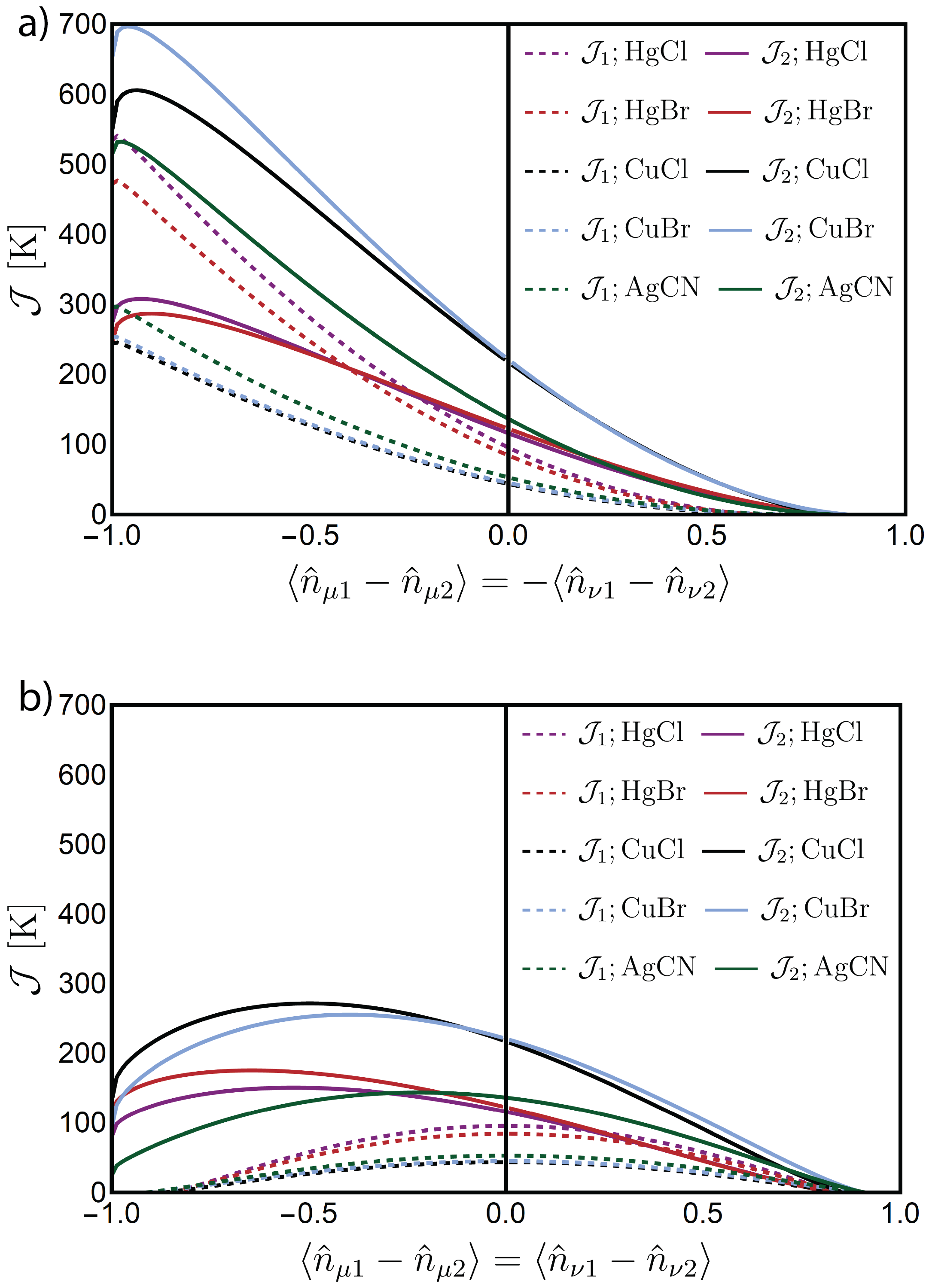
Figure 4: Variation of the effective interdimer superexchange interaction with the charge disproportionation, $\langle\hat{n}_{\mu 1}-\hat{n}_{\mu 2}\rangle$, for (a) antiferrodipolar ordering and (b) ferrodipolar ordering. For ease of comparison both panels use the same axis scales.

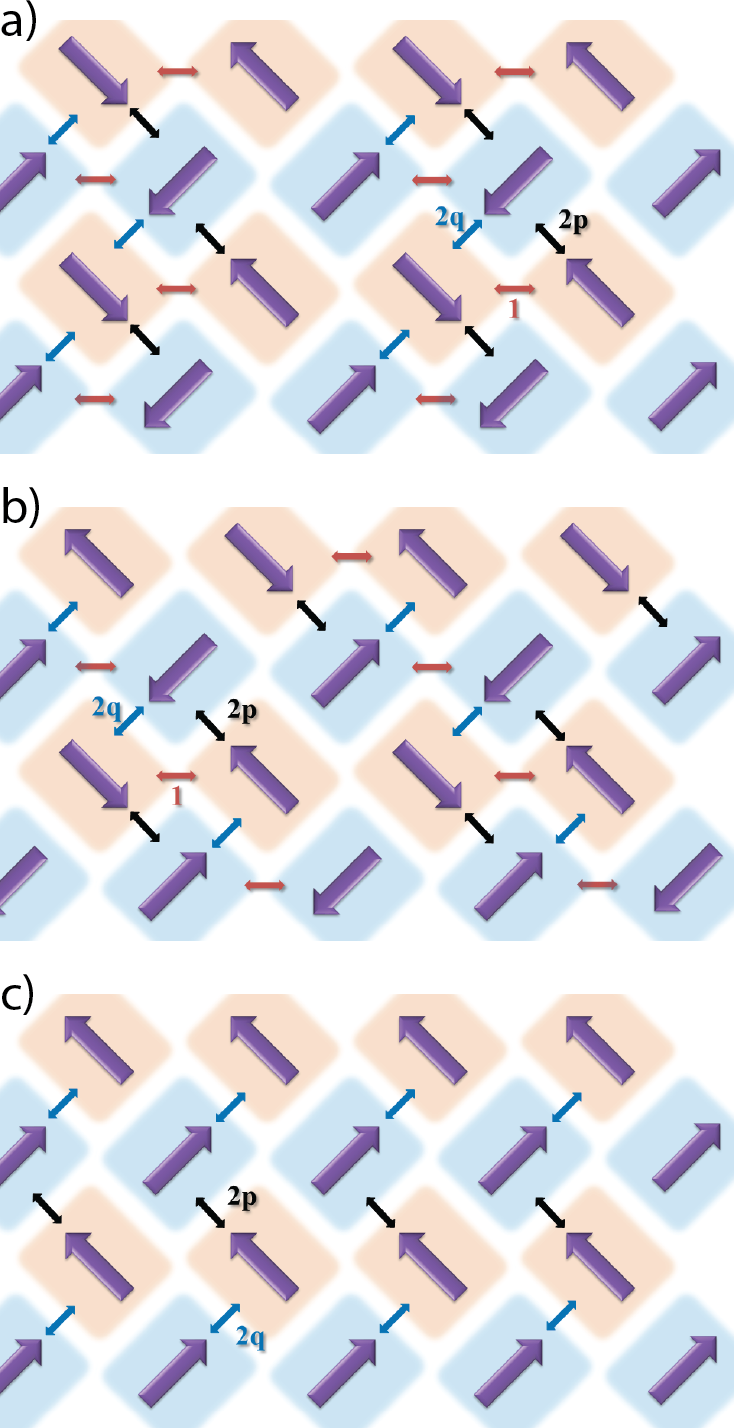
Figure 5: Possible dipole ordering patterns (a,b) in the quasi-one-dimensional limit of the TFIM ($K_{1}\gg K_{2}$) and (c) in the square lattice limit of the TFIM, ($K_{2}\gg K_{1}$). The head of the arrows indicates the monomer that contains fewer electrons than the monomer at the tail of the arrow. To understand the microscopic dipolar order shown here it is helpfull to compare with Fig. 1. Only the supperexchange interactions that are strongest when the dipoles order are marked in this figure. In all cases strong charge disproportionation combined with dipole order leads to a quasi-one-dimensional spin system.

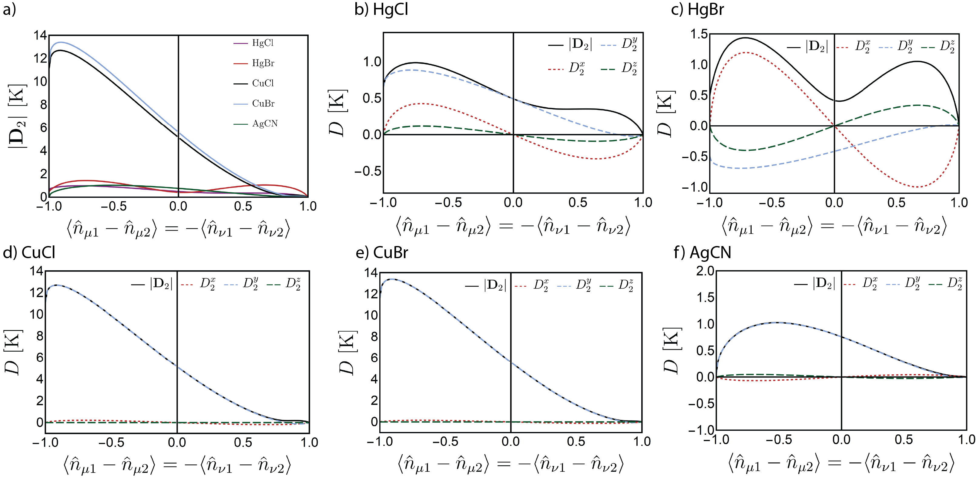
Figure 6: Variation of the effective interdimer Dzyaloshinskii-Moriya antisymmetric exchange with the charge disproportionation, $\hat{n}_{\mu 1}-\hat{n}_{\mu 2}$, for an antiferrodipolar configuration of dimers. a) Magnitude for all materials and Cartesian components for b) $\kappa$-HgCl, c) $\kappa$-HgBr, d) $\kappa$-CuCl, e) $\kappa$-CuBr, and f) $\kappa$-AgCN.

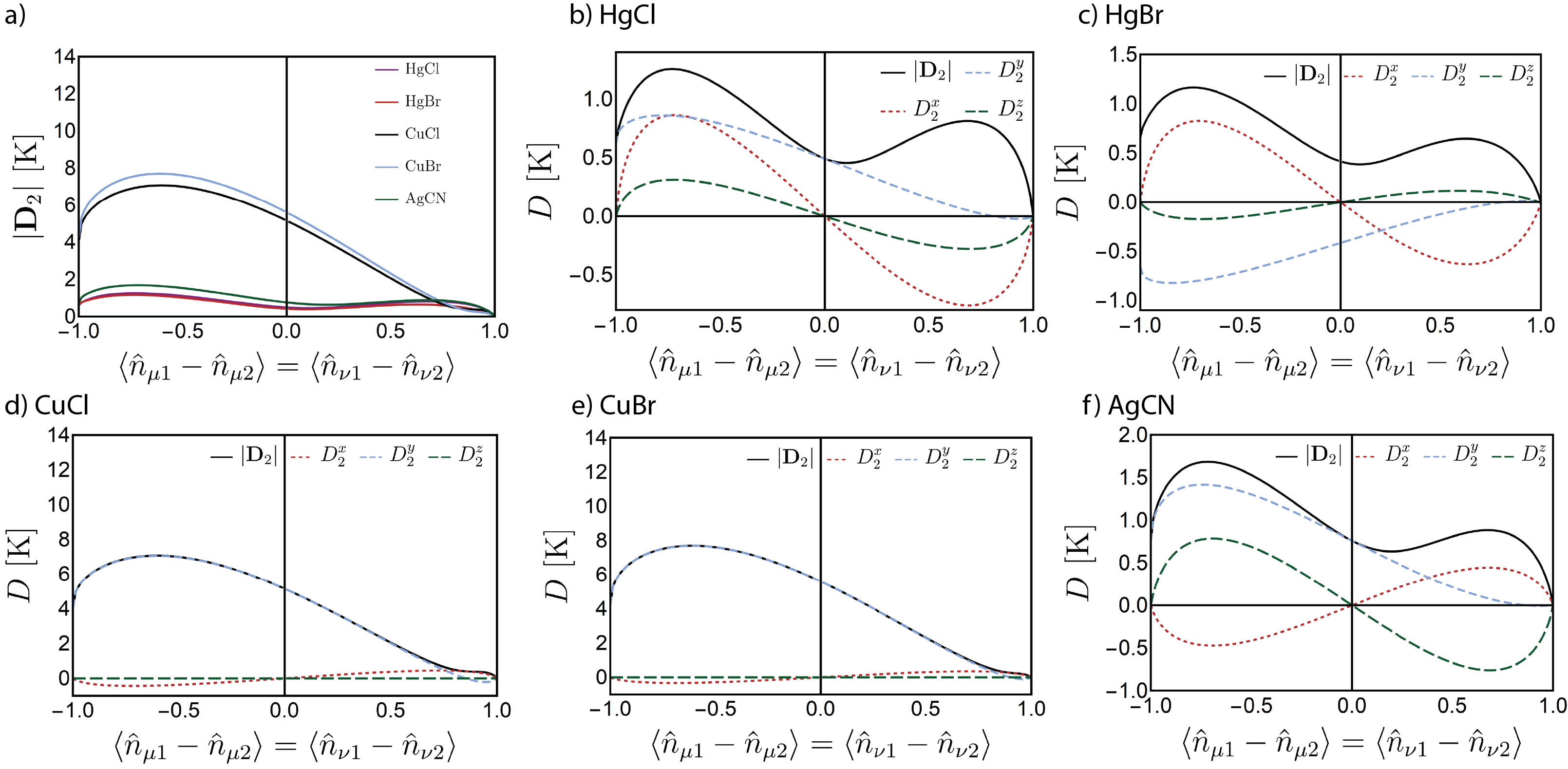
Figure 7: Variation of the effective interdimer Dzyaloshinskii-Moriya antisymmetric exchange with the charge disproportionation, $\hat{n}_{\mu 1}-\hat{n}_{\mu 2}$, for a ferrodipolar configuration of dimers. a) Magnitude for all materials and Cartesian components for b) $\kappa$-HgCl, c) $\kappa$-HgBr, d) $\kappa$-CuCl, e) $\kappa$-CuBr, and f) $\kappa$-AgCN.

In both cases the variation of the interdimer superexchange with charge disproportionation is extremely dramatic. This is a simple consequence of the dependence of the perturbative processes, in the monomer model (Fig. 3), on the occupation of the two different Wanniers, which is easily understood by considering the limits $\langle\hat{n}_{\mu 1}-\hat{n}_{\mu 2}\rangle\rightarrow\pm 1$.

Notice that superexchange interactions vanish for $\langle\hat{n}_{\mu 1}-\hat{n}_{\mu 2}\rangle\rightarrow 1$ in both the antiferrodiplar and ferrodipolar cases. This can easily be understood by examining the form of the interdimer hopping, Eqs. (8) and (10), and Fig. 3. Clearly, all virtual hopping processes between the dimers cease when $\langle\hat{n}_{\mu 1}-\hat{n}_{\mu 2}\rangle\rightarrow 1$ as they require a partial occupation of monomer $\mu 2$.

For $\langle\hat{n}_{\mu 1}-\hat{n}_{\mu 2}\rangle\rightarrow-1$ each of the cases gives a different result. ${\cal J}_{1}=0$ in the ferrodipolar case. This is again a straightforward consequence of the detailed form of the interdimer hopping, Eq. (8) see also Fig. 3, which shows that superexchange via the $t_{b2}$ pathway requires partial occupation of Wannier $\nu 1$, which is doubly occupied in this limit. In the antiferrodipolar case ${\cal J}_{1}\not\rightarrow 0$ for $\langle\hat{n}_{\mu 1}-\hat{n}_{\mu 2}\rangle\rightarrow-1$. In this limit $\langle\hat{n}_{\mu 2}\rangle=\langle\hat{n}_{\nu 1}\rangle\rightarrow 1$ and the second order perturbation due to $t_{b2}$, Eq. (8), reduces to the usual case of superexchange between two half-filled sites Powell (2011). Similarly ${\cal J}_{2}$ simplifies to the problem of superexchange between two half-filled sites when $\langle\hat{n}_{\mu 1}-\hat{n}_{\mu 2}\rangle\rightarrow-1$. For an antiferrodipolar arrangement ${\cal J}_{2}\rightarrow{\cal J}_{2p}\propto t_{p}^{2}$ and for a ferrodipolar arrangement ${\cal J}_{2}\rightarrow{\cal J}_{2q}\propto t_{q}^{2}$ and hence ${\cal J}_{2p}>{\cal J}_{2q}$.

To understand the impact of dipole order on the magnetic properties it is important to know which long-range pattern of dipoles is realized. The solution of the TFIM, Eq. (12), is an extremely challenging problem and beyond the scope of this Article. But, for illustrative purposes it is useful to consider the order in the classical zero-field regime. Two low-energy states for $K_{1}\gg K_{2}$ are sketched in Figs. 5a and b, and the lowest energy state for $K_{2}\gg K_{1}$ is sketched in Fig. 5c. In all cases we have marked only the strongest magnetic superexchange interactions. The magnetic interactions that are not shown are zero for complete charge disproportionation $|\langle\hat{n}_{\mu 1}-\hat{n}_{\mu 2}\rangle|\rightarrow 1$, but simply small in the more realistic case of incomplete charge disproportionation $0<|\langle\hat{n}_{\mu 1}-\hat{n}_{\mu 2}\rangle|<1$. The values of the ‘large’ and ‘small’ interactions correspond to changing the sign of charge disproportionation $\langle\hat{n}_{\mu 1}-\hat{n}_{\mu 2}\rangle$ in Fig. 4.

The order sketched in Figs. 5a and b are relevant to $\kappa$-HgCl and $\kappa$-HgBr. Our calculations suggest that these are very close in energy, with the very weak $W^{TT}_{3}$ interaction, cf. Table 2, favoring the order sketched in 5b. However, the existence of competing orders very interesting given the recent observation of dipole liquid-like behaviors in $\kappa$-HgBr Hassan et al. (2018). This suggests the possibility of resonance structures similar to those proposed in spin liquids Powell (2018); Anderson (1987).

In the dipole orders sketched in Fig. 5 the ‘strong’ bonds form quasi-one-dimensional spin systems, coupled by the ‘weak’ bonds. The effects of this anisotropy will depend strongly on the difference between the $\cal J$ values of the ‘strong’ and ‘weak’ bonds, which is in turn determined by the magnitude of the charge disproportionation. The resulting spin model could range from a subtly anisotropic quasi-two-dimensional system (for weak charge disproportionation) to quasi-one-dimensional spin systems (for large charge disproportionation). However, we note that the geometrical frustration of the magnetic interactions means that this quasi-one-dimensional limit is more stable than one might naively expect Powell et al. (2017b); Kenny et al. (2019a, b). Therefore, the effective one-dimensionalization of the system when it is dipole ordered could be important for understand the large “dipole-solid+spin-liquid” phase found by Hotta in her exact diagonalization studies of the NIH model Hotta (2010).

Similarly, the vector hopping between the different sublattices (cf. Table 1) induces a Dzyaloshinskii-Moriya antisymmetric exchange interaction:

$$\hat{H}_{\text{DM}}=\sum_{\langle\mu,\nu\rangle}{\bm{D}}_{1}\cdot\hat{\bm{S}}_{\mu}\times\hat{\bm{S}}_{\nu}+\sum_{[\mu,\nu]}{\bm{D}}_{2}\cdot\hat{\bm{S}}_{\mu}\times\hat{\bm{S}}_{\nu}.$$ (19)

This is calculated as described in Powell et al. (2017a) and plotted in Fig. 6, for an antiferrodipolar arrangement, and Fig. 7, for an ferrodipolar arrangement. ${\bm{D}}_{1}=\bm{0}$ in all materials because there is an inversion symmetry between the dimers on the same sublattice. The Dzyaloshinskii-Moriya interaction is likely to be profoundly important for determining the macroscopic magnetic properties because of the low dimensionality of the system Mermin and Wagner (1966).

Regardless of the degree of charge order, the Dzyaloshinskii-Moriya interaction is much stronger in $\kappa$-CuBr and $\kappa$-CuCl than it is in $\kappa$-AgCN. This is interesting because the former pair both order antiferromagnetically, whereas the long-range magnetic order has not been observed in $\kappa$-AgCN at any temperature. The Mermin-Wagner theorem Mermin and Wagner (1966) shows that there cannot be long-range order in two-dimensional Heisenberg model, but a Dzyaloshinskii-Moriya interaction violates the assumptions required to prove the theorem and allows for long-range magnetic order. Therefore, a natural perspective on these materials, given the very week interlayer interactions, is that the absence of long-range order is the natural state of affairs; and that a significant Dzyaloshinskii-Moriya interaction is required to cause long-range order.

Finally we note that, in several compounds, dipole ordering significantly increases the Dzyaloshinskii-Moriya coupling. Thus, dipole order could cause or enhance long-range antiferromagnetic order.

V Conclusions

In summary, we have used a combination of first principles calculations and empirical relationships for the Coulomb interactions to parameterize the HIN model of coupled dipolar and spin degrees of freedom for $\kappa$-HgCl, $\kappa$-HgBr, $\kappa$-CuCl, $\kappa$-CuBr, and $\kappa$-AgCN. In all materials the coupling constants for the TFIM of the dipoles are the largest energy scales in the problem. This quantifies, justifies and confirms recent claims that the dipoles are of crucial importance for understanding these materials Clay and Mazumdar (2019); Hotta (2010); Naka and Ishihara (2010); Lunkenheimer et al. (2012); Abdel-Jawad et al. (2010); Iguchi et al. (2013).

Two effects are responsible for different ferroelectric behaviors of the $\kappa$-(BEDT-TTF)${}_{2}X$ salts. (i) The inter-dimer hopping, $t_{b1}$, which gives rise to the “transverse field” in the Ising model for the dipoles ($H^{T}=2t_{b1}$), is between a third and a tenth smaller in $\kappa$-HgCl and $\kappa$-HgBr than in $\kappa$-CuCl, $\kappa$-CuBr, and $\kappa$-AgCN. (ii) The TFIM of dipoles is in the quasi-one-dimensional limit for $\kappa$-HgCl and $\kappa$-HgBr, but quasi-two-dimensional (between the square and isotropic triangular limits) for $\kappa$-CuCl, $\kappa$-CuBr, and $\kappa$-AgCN. Thus, the dimensionless critical field is 3 – 5 times smaller in the former pair of compounds. Clearly then, effect (ii) is much more important for this conclusion than effect (i). This occurs because $X_{TT}\propto t_{b2}^{2}$ [see Eq. (26)] and $t_{b2}$ is 25-50% larger in $\kappa$-HgCl and $\kappa$-HgBr than the other materials, see Table 1, which means that $X_{TT}$ is much bigger in the mercuric materials. $Y_{TT}\propto(t_{p}^{2}-t_{q}^{2})$ [see Eq. (31)] and $t_{p}$ is $\sim 50\%$ larger in the non-mercuric materials, which results in a much larger $Y_{TT}$ in these systems.

We have also found that dipolar order and even short-range dipolar correlations have a profound impact on the nature of the interdimer magnetic (superexchange) interactions. In particular for dipole crystals this appears to drive the materials towards quasi-one-dimensional magnetic interactions, which could be important for understand the spin liquids found in many of these materials. Conversely, dipole order can increase with Dzyaloshinskii-Moriya interaction, which may tend to stabilize magnetic order. Understanding the interplay of these effects is a significant challenge for future quantum many-body theories.

Appendix A Parameters in Eqs. (9) and (11)

The simplest method to calculate the contributions to the effective spin-dipole Hamiltonian at second order in $\hat{H}_{1}$ and $\hat{H}_{2}$ is to make use of projectors. Recall that the spin operator

$$\hat{P}_{0}\equiv\frac{1}{4}-\bm{S}_{1}\cdot\bm{S}_{2}=\left\{\begin{array}[]{ll}1&\text{if the spins form a singlet}\\ 0&\text{if the spins form a triplet,}\end{array}\right.$$ (22)

and

$$\hat{P}_{1}\equiv\bm{S}_{1}\cdot\bm{S}_{2}+\frac{3}{4}=\left\{\begin{array}[]{ll}0&\text{if the spins form a singlet}\\ 1&\text{if the spins form a triplet,}\end{array}\right.\,$$ (25)

Similarly, $\hat{P}_{\pm}\equiv T^{z}\pm\frac{1}{2}$ projects the unpaired electron on to monomers 1 ($-$) and 2 ($+$). These four projectors and the operators $T^{\pm}=T^{x}\pm iT^{y}$ make it straightforward, but tedious, to enumerate all possible second order corrections in the scalar hopping parameters, Eqs. (8) and (10), and rearrange into the form of the effective Hamiltonains, Eqs. (9) and (11). Whence, one finds that

$$X_{TT} = \frac{t_{b2}^{2}}{U}+\frac{t_{b2}^{2}\left(2V_{b1}+7J_{b1}\right)}{V_{b1}\left(V_{b1}-2J_{b1}\right)},$$ (26)

$$X_{T} = -\frac{t_{b2}^{2}}{2U},$$ (27)

$$X_{SSTT} = \frac{4t_{b2}^{2}}{U}-\frac{4t_{b2}^{2}J_{b1}}{V_{b1}\left(V_{b1}-2J_{b1}\right)},$$ (28)

$$X_{SST} = -\frac{2t_{b2}^{2}}{U},$$ (29)

$$X_{SS} = \frac{t_{b2}^{2}J_{b1}}{V_{b1}\left(V_{b1}-2J_{b1}\right)},$$ (30)

$$Y_{TT} = \frac{(t_{p}^{2}-t_{q}^{2})}{U}+\frac{(t_{p}^{2}-t_{q}^{2})(2V_{b1}+7J_{b1})}{V_{b1}\left(V_{b1}-2J_{b1}\right)},$$ (31)

$$Y_{zx} = -\frac{t_{p}t_{q}}{2U}-\frac{t_{p}t_{q}(2V_{b1}+7J_{b1})}{2V_{b1}\left(V_{b1}-2J_{b1}\right)},$$ (32)

$$Y_{T-} = -\frac{t_{p}^{2}}{2U},$$ (33)

$$Y_{T+} = -\frac{t_{q}^{2}}{2U},$$ (34)

$$Y_{x} = -\frac{t_{p}t_{q}}{4U}-\frac{t_{p}t_{q}(2V_{b1}+7J_{b1})}{4V_{b1}\left(V_{b1}-2J_{b1}\right)}$$ (35)

$$Y_{SSTT} = \frac{4(t_{p}^{2}-t_{q}^{2})}{U}-\frac{4(t_{p}^{2}-t_{q}^{2})J_{b1}}{V_{b1}\left(V_{b1}-2J_{b1}\right)},$$ (36)

$$Y_{SSzx} = \frac{2t_{p}t_{q}}{U}-\frac{t_{p}t_{q}(V_{b1}+J_{b1})}{V_{b1}\left(V_{b1}-2J_{b1}\right)}$$ (37)

$$Y_{SST-} = -\frac{2t_{p}^{2}}{U},$$ (38)

$$Y_{SST+} = -\frac{2t_{q}^{2}}{U},$$ (39)

$$Y_{SSx} = \frac{t_{p}t_{q}}{U}-\frac{t_{p}t_{q}(V_{b1}+J_{b1})}{V_{b1}\left(V_{b1}-2J_{b1}\right)},$$ (40)

$$Y_{SS} = \frac{(t_{p}^{2}+t_{q}^{2})J_{b1}}{V_{b1}\left(V_{b1}-2J_{b1}\right)},$$ (41)

$$Y_{4Szx} = \frac{8t_{p}t_{q}J_{b1}}{V_{b1}\left(V_{b1}-2J_{b1}\right)},$$ (42)

and

$$Y_{4Sx} = \frac{4t_{p}t_{q}J_{b1}}{V_{b1}\left(V_{b1}-2J_{b1}\right)}.$$ (43)

References

- Kino and Fukuyama (1996) H. Kino and H. Fukuyama, J. Phys. Soc. Japan 65, 2158 (1996).
- McKenzie (1998) R. H. McKenzie, Comments Cond. Mat. Phys. 18, 309 (1998).
- Powell and McKenzie (2006) B. J. Powell and R. H. McKenzie, J. Phys.: Cond. Matt. 18, R827 (2006).
- Powell and McKenzie (2011) B. J. Powell and R. H. McKenzie, Rep. Prog. Phys. 74, 056501 (2011).
- Clay and Mazumdar (2019) R. Clay and S. Mazumdar, Physics Reports 788, 1 (2019).
- Hotta (2010) C. Hotta, Phys. Rev. B 82, 241104 (2010).
- Naka and Ishihara (2010) M. Naka and S. Ishihara, Journal of the Physical Society of Japan 79, 063707 (2010).
- Lunkenheimer et al. (2012) P. Lunkenheimer, J. Müller, S. Krohns, F. Schrettle, A. Loidl, B. Hartmann, R. Rommel, M. de Souza, C. Hotta, J. A. Schlueter, et al., Nature Materials 11, 755 (2012).
- Iguchi et al. (2013) S. Iguchi, S. Sasaki, N. Yoneyama, H. Taniguchi, T. Nishizaki, and T. Sasaki, Phys. Rev. B 87, 075107 (2013).
- Abdel-Jawad et al. (2010) M. Abdel-Jawad, I. Terasaki, T. Sasaki, N. Yoneyama, N. Kobayashi, Y. Uesu, and C. Hotta, Phys. Rev. B 82, 125119 (2010).
- Drichko et al. (2014) N. Drichko, R. Beyer, E. Rose, M. Dressel, J. A. Schlueter, S. A. Turunova, E. I. Zhilyaeva, and R. N. Lyubovskaya, Phys. Rev. B 89, 075133 (2014).
- Gati et al. (2018) E. Gati, J. K. H. Fischer, P. Lunkenheimer, D. Zielke, S. Köhler, F. Kolb, H.-A. K. von Nidda, S. M. Winter, H. Schubert, J. A. Schlueter, et al., Phys. Rev. Lett. 120, 247601 (2018).
- Hassan et al. (2018) N. Hassan, S. Cunningham, M. Mourigal, E. I. Zhilyaeva, S. A. Torunova, R. N. Lyubovskaya, J. A. Schlueter, and N. Drichko, Science 360, 1101 (2018).
- Seo et al. (2004) H. Seo, C. Hotta, and H. Fukuyama, Chemical Reviews 104, 5005 (2004).
- Pavarini (2016) E. Pavarini, Orbital Ordering (Verlag des Forschungszentrum Jülich, 2016), vol. 6 of Modeling and Simulation, chap. 7, URL https://www.cond-mat.de/events/correl16/manuscripts/pavarini.pdf.
- Blöte and Deng (2002) H. W. J. Blöte and Y. Deng, Phys. Rev. E 66, 066110 (2002).
- du Croo de Jongh and van Leeuwen (1998) M. S. L. du Croo de Jongh and J. M. J. van Leeuwen, Phys. Rev. B 57, 8494 (1998).
- Eschrig et al. (2004) H. Eschrig, M. Richter, and I. Opahle, in Theoretical and Computational Chemistry, edited by P. Schwerdtfeger (Elsevier, 2004), chap. 12: Relativistic solid state calculations, pp. 723–776.
- Koepernik and Eschrig (1999) K. Koepernik and H. Eschrig, Phys. Rev. B 59, 1743 (1999).
- Taniguchi et al. (1999) H. Taniguchi, A. Kawamoto, and K. Kanoda, Phys. Rev. B 59, 8424 (1999).
- Perdew et al. (1996) J. P. Perdew, K. Burke, and M. Ernzerhof, Phys. Rev. Lett. 77, 3865 (1996).
- Schlueter (2018) J. A. Schlueter, private communication (2018).
- Geiser et al. (1991a) U. Geiser, A. J. Schults, H. H. Wang, D. M. Watkins, D. L. Stupka, J. M. Williams, J. Schirber, D. Overmyer, D. Jung, J. Novoa, et al., Physica C: Superconductivity 174, 475 (1991a).
- Geiser et al. (1991b) U. Geiser, A. M. Kini, H. H. Wang, M. A. Beno, and J. M. Williams, Acta Crystallographica Section C 47, 190 (1991b).
- Saito (2015) G. Saito, private communication (2015).
- Koretsune and Hotta (2014) T. Koretsune and C. Hotta, Phys. Rev. B 89, 045102 (2014).
- Shinaoka et al. (2012) H. Shinaoka, T. Misawa, K. Nakamura, and M. Imada, Journal of the Physical Society of Japan 81, 034701 (2012).
- Nakamura et al. (2009) K. Nakamura, Y. Yoshimoto, T. Kosugi, R. Arita, and M. Imada, Journal of the Physical Society of Japan 78, 083710 (2009).
- Nakamura et al. (2012) K. Nakamura, Y. Yoshimoto, and M. Imada, Phys. Rev. B 86, 205117 (2012).
- Weihong et al. (1999) Z. Weihong, R. H. McKenzie, and R. R. P. Singh, Phys. Rev. B 59, 14367 (1999).
- Scriven and Powell (2012) E. P. Scriven and B. J. Powell, Phys. Rev. Lett. 109, 097206 (2012).
- Powell et al. (2017a) B. J. Powell, J. Merino, A. L. Khosla, and A. C. Jacko, Phys. Rev. B 95, 094432 (2017a).
- Powell et al. (2017b) B. J. Powell, E. Kenny, and J. Merino, Phys. Rev. Lett. 119, 087204 (2017b).
- Powell (2011) B. J. Powell, in Computational Methods for Large Systems: Electronic Structure Approaches for Biotechnology and Nanotechnology, edited by J. R. Reimers (Wiley, Hoboken, 2011), chap. 10: An introduction to effective low-energy Hamiltonians in condensed matter physics and chemistry, pp. 309–366, eprint arXiv:0906.1640.
- Powell (2018) B. J. Powell, Science 360, 1073 (2018).
- Anderson (1987) P. W. Anderson, Science 235, 1196 (1987).
- Kenny et al. (2019a) E. P. Kenny, G. David, N. Ferré, A. C. Jacko, and B. J. Powell, arXiv:1909.10222 (2019a).
- Kenny et al. (2019b) E. P. Kenny, A. C. Jacko, and B. J. Powell, Angew. Chem. Int. Ed., in press, doi:10.1002/anie.201907889 (2019b).
- Mermin and Wagner (1966) N. D. Mermin and H. Wagner, Phys. Rev. Lett. 17, 1133 (1966).