The Trimmed Mean in Non-parametric Regression Function Estimation

Abstract

This article studies a trimmed version of the Nadaraya-Watson estimator to estimate the unknown non-parametric regression function. The characterization of the estimator through minimization problem is established, and its pointwise asymptotic distribution is derived. The robustness property of the proposed estimator is also studied through breakdown point. Moreover, as the trimmed mean in the location model, here also for a wide range of trimming proportion, the proposed estimator poses good efficiency and high breakdown point for various cases, which is out of the ordinary property for any estimator. Furthermore, the usefulness of the proposed estimator is shown for three benchmark real data and various simulated data.

Keywords: Heavy-tailed distribution; Kernel density estimator; $L$-estimator; Nadaraya-Watson estimator; Robust estimator.

1 Introduction

We have a random sample $(X_{1},Y_{1}),\ldots,(X_{n},Y_{n})$, which are i.i.d. copies of $(X,Y)$, and the regression of $Y$ on $X$ is defined as

$$Y_{i}=g(X_{i})+e_{i},\quad i=1,\ldots,n,$$ (1)

where $g(\cdot)$ is unknown, and $e_{i}$ are independent copies of error random variable $e$ with $E(e\,|\,X)=0$ and $var(e\,|\,X=x)=\sigma^{2}(x)<\infty$ for all $x$. Note that the condition $E(e\,|\,X)=0$ is essentially the identifiable condition for mean regression, and it varies over the different procedures of regression. For instance, in the case of the median regression, the identifiable condition will be the median functional $(e|X)=0$ or for the trimmed mean regression, it will be the trimmed mean functional $(e|X)=0$.

There have been several attempts to estimate the unknown non-parametric regression function $g(\cdot)$; for overall exposure on this topic, the readers are referred to priestley1972non, clark1977non and gasser1979kernel. Among well-known estimators of the regression function, the Nadaarya-Watson estimator (see nadaraya1965non and watson1964smooth ) is one of the most classical estimator, and it has been used in different Statistical methodologies. Some other classical estimators of the regression function, namely, Gasser-Müller Gasser  Müller (1979) and Priestley-Chao Priestley  Chao (1972) estimators are also well-known in the literature. In this context, we should mention that all three aforesaid estimators are based on kernel function; in other words, these estimators are examples of kernel smoothing of regression function. In fact more generally speaking, one may consider local polynomial fitting as a kernel regression smoother, and the fact is that Nadaraya-Watson estimator is nothing but a local constant kernel smoother.

Note that as it is mentioned in the previous paragraph, Nadaraya-Watson estimator can be obtained from a certain minimization problem related to the weighted least squares methodology, where the weights are the functional values of the kernel function evaluated at data points. This fact further indicates that it is likely to be less efficient in the presence of the outliers or influential observations in the data. To overcome this problem, we here propose the trimmed version of Nadaraya-Watson estimator, which can be obtained as the minimizer of a certain minimization problem. It is also of interest to see how this estimator performs compared to the classical Nadaraya-Watson estimator (i.e., based on the usual least squares methodology) when data follow various distributions. For instance, it should be mentioned that for the location parameter of Cauchy distribution, neither the sample mean nor the sample median, 0.38-trimmed mean is the most efficient estimator for the location parameter of Cauchy distribution as pointed out by dhar2016trimmed. In fact, such a nice combination of efficiency and robustness properties of the trimmed mean for various Statistical model (see, e.g., dhar2009comparison,dhar2012derivatives, dhar2016trimmed, vcivzek2016generalized, park2015robust, wang2019robust and references therein) motivated us to propose this estimator and study its behaviour. For the classical references of the trimmed mean, one may look at bickel1965some, hogg1967some, jaeckel1971some, stigler1973asymptotic, welsh1987trimmed, jureckova1994regression and jurevckova1994adaptive.

The contribution of this article is three fold. The first fold is to propose an entirely new estimator of the non-parametric regression function, which was never studied in the literature before. The next fold is the derivation of the asymptotic distribution of the proposed estimator. As the proposed estimator is based on the order statistic, one cannot use the classical central limit theorem directly; it requires advanced technicalities associated with order statistic to obtain the asymptotic distribution. The last fold is the formal study of the robustness property of the proposed estimator using the concept of breakdown point.

As said before, one of the main crux of the problem is to show the proposed estimator as a minimizer of a certain minimization problem, and that enables us to explain the geometric feature of the estimator. Besides, another difficulty involved in deriving the asymptotic distribution is dealing the order statistics in the non-parametric regression set up. For this reason, one cannot use the classical central limit theorem to establish the asymptotic normality of the estimator after appropriate normalization. Moreover, the presence of kernel function in the expression of the estimator also made challenging to establish the breakdown point of the estimator.

The rest of this article is arranged as follows. Section 2 proposes the estimator and shows how it obtains from the minimization problem. Section 3 provides the large sample properties of the proposed estimator, and the robustness property of the estimator is studied in Section 4. Section 5 presents the finite sample study, and the performance of the estimator for a few benchmark data set is shown in Section 6. Section 7 contains a few concluding remarks. The proof of Theorem 3.1 along with the related lemmas is provided in Appendix A, and Appendix B contains all results of numerical studies in tabular form.

2 Proposed Estimator

Let $(X_{1},Y_{1}),\ldots,(X_{n},Y_{n})$ be an i.i.d. sequence of random variables having the same joint distribution of $(X,Y)$ and recall the model (1). The well-known Nadaraya-Watson estimator is defined as

$$\hat{g}_{n,NW}(x_{0})=\frac{\sum\limits_{i=1}^{n}k_{n}\left(X_{i}-x_{0}\right)Y_{i}}{\sum\limits_{i=1}^{n}k_{n}\left(X_{i}-x_{0}\right)},$$

where $\displaystyle k_{n}(\cdot)=\frac{1}{h_{n}}K\left(\frac{\cdot}{h_{n}}\right)$, and $K(\cdot)$ is a symmetric kernel function, i.e., $K$ is a non negative kernel with support $[-\tau,\tau]$, $\displaystyle\int\limits_{-\tau}^{\tau}K(u)du=1$ and $K(-u)=K(u)$ for all $u\in[-\tau,\tau]$. Besides, $\{h_{n}\}$ is a sequence of bandwidth, such that $h_{n}\rightarrow 0$ as $n\rightarrow\infty$ and $nh_{n}\rightarrow\infty$ as $n\rightarrow\infty$. Note that $\hat{g}_{n,NW}(x_{0})$ can be expressed as a solution of the following minimization problem :

$$\hat{g}_{n,NW}(x_{0})=\operatorname*{arg\,min}\limits_{\theta}\sum\limits_{i=1}^{n}\left(Y_{i}-\theta\right)^{2}k_{n}\left(X_{i}-x_{0}\right).$$ (2)

Note that the above formulation implies that Nadaraya-Watson estimator is a certain weighted average estimator, which can be obtained by weighted least squares methodology. It is a well-known fact that the (weighted) least squares methodology is not robust against the outliers or influential observations (see, e.g., huber1981robust), and to overcome this problem related to the robustness against the outliers, we here study the trimmed version of the weighted least squares methodology, which obtains the local constant trimmed estimator of the non-parametric regression function, i.e., the trimmed version of Nadaraya-Watson estimator. Let us now define the estimator formally, which is denoted by $\hat{g}_{n,\alpha}(\cdot)$ for $\alpha\in[0,\frac{1}{2})$.

$$\hat{g}_{n,\alpha}(x_{0})=\operatorname*{arg\,min}\limits_{\theta}\sum\limits_{i=[n\alpha]+1}^{n-[n\alpha]}\left(Y_{[i]}-\theta\right)^{2}k_{n}\left(X_{(i)}-x_{0}\right),$$ (3)

where $X_{(i)}$ is the $i$-th ordered observation on variable $X$, and $Y_{[i]}$ denotes the observation on variable $Y$ corresponding $X_{(i)}$. Solving (3), we have

$$\hat{g}_{n,\alpha}(x_{0})=\frac{\sum\limits_{i=[n\alpha]+1}^{n-[n\alpha]}k_{n}\left(X_{(i)}-x_{0}\right)Y_{[i]}}{\sum\limits_{i=[n\alpha]+1}^{n-[n\alpha]}k_{n}\left(X_{(i)}-x_{0}\right)}.$$ (4)

Here it should be mentioned that $\alpha\in[0,\frac{1}{2})$ is the trimming proportion, and in particular, for $\alpha=0$, $\hat{g}_{n,\alpha}(\cdot)$ will coincide with $\hat{g}_{n,NW}(\cdot)$. i.e., usual Nadaraya-Watson estimator. Further, note that here $Y_{[i]}=g(X_{(i)})+e_{[i]}$ for $i=1,\ldots,n$, where $e_{[i]}$ denotes the error corresponding to $(X_{(i)},Y_{[i]})$.

We now want to add one discussion on possible extension of this estimator. As it follows from (2), Nadaraya-Watson estimator is a local constant estimator, and in this context, it should be added that there has been an extensive literature on local linear (strictly speaking, local polynomial) estimator of non-parametric regression function. One of the advantage of local linear or generally speaking local polynomial estimator is, it gives a consistent estimator of a certain order derivatives of the regression function as well (see, e.g., fan1996local) but on the other hand, it will enhance the overall standard error as well. Following the same spirit, one can consider local linear or polynomial trimmed mean of non-parametric regression function, and it will be an interest of future research.

This section ends with another discussion on the choice of the tuning parameter $\alpha$ involved in $\hat{g}_{n,\alpha}(x_{0})$. Apparently, our efficiency study (see in Section 3.1) and simulation study (see in Section 5) indicate that for a wide range of $\alpha$, $\hat{g}_{n,\alpha}(x_{0})$ has good efficiency property for various distributions. In contrast, in terms of the robustness against the outliers, $\hat{g}_{n,\alpha}(x_{0})$ attains the highest breakdown point when $\alpha$ attains its largest value (see Section 4). However, since there is a trade-off between efficiency and robustness of an estimator, choosing the largest value of $\alpha$ in practice may originate an estimator having poor efficiency. In order to maintain the best efficiency and a reasonably good breakdown point, one may estimate the trimming proportion $\alpha$ (denote it as $\hat{\alpha}$), which minimizes the estimated asymptotic variance of $\hat{g}_{n,\alpha}(x_{0})$ after appropriate normalization. However, Statistical methodology based on $\hat{g}_{n,\hat{\alpha}}(x_{0})$ will be difficult to implement because of its intractable nature. Overall, the choice of $\alpha$ is an issue of concern to use $\hat{g}_{n,\alpha}(x_{0})$ in practice.

3 Asymptotic distribution of $\hat{g}_{n,\alpha}(\cdot)$

In order to implement any Statistical methodology based on $\hat{g}_{n,\alpha}(\cdot)$, one needs to know the distributional behaviour of $\hat{g}_{n,\alpha}(\cdot)$. However, due to complicated form of $\hat{g}_{n,\alpha}(\cdot)$, it is intractable to derive the exact distribution, which drives us to study the asymptotic distribution of $\hat{g}_{n,\alpha}(\cdot)$. This section describes the pointwise asymptotic distribution of $\hat{g}_{n,\alpha}(\cdot)$ after appropriate normalization. To prove the main result, one needs to assume the following conditions.

Assumptions :

• The regression function $g(\cdot)$ is a real valued continuously twice differentiable function on a compact set.

• The probability density function of the covariate random variable $X$, which is denoted by $f_{X}$, is a bounded function.

• The kernel $K(\cdot)$ is a bounded probability density function with support $(-\tau,\tau)$ such that,
  (a) $\displaystyle\int_{-\tau}^{\tau}K(u)du=1$,
  (b) $\displaystyle\int_{-\tau}^{\tau}uK(u)du=0$, and
  (c) $\displaystyle h_{n}^{-1}K\left(h_{n}^{-1}\right)=O(1)$.

• The sequence of bandwidth $\{h_{n}\}$ is such that $h_{n}=O(n^{-1/3})$.

• The probability density function of error random variable $e$ is symmetric about $0$ with the following properties:

  (i) $e_{i}$s are i.i.d. random variables.

  (ii) For the location functional $T(F)$, $T(F_{e|X})=0$, where $F_{e|X}$ is the conditional distribution of $e$ conditioning on $X$. For instance, in the case of $\alpha$-trimmed mean, $T(F)=\frac{1}{(1-2\alpha)}\int xdF(x)$, where $\alpha\in[0,\frac{1}{2})$.

  (iii) $E({e}^{2}|\,X=x)=\sigma^{2}(x)<\infty$ for all $x$.

• There exists a positive $\delta$ such that $E(|e_{i}|^{2+\delta})<\infty$ for all $i=1,\ldots,n$.

Theorem 3.1.

Under (A1)-(A6) and for any fixed point $x_{0}$,

$$\sqrt{nh_{n}}\left(\hat{g}_{n,\alpha}(x_{0})-g(x_{0})-h_{n}^{2}k_{2}\left(\frac{g^{\prime\prime}(x_{0})}{2(n-2[n\alpha])}\sum\limits_{i=[n\alpha]+1}^{n-[n\alpha]}f_{X_{(i)}}(x_{0})+\frac{g^{\prime}(x_{0})}{(n-2[n\alpha])}\sum\limits_{i=[n\alpha]+1}^{n-[n\alpha]}f^{\prime}_{X_{(i)}}(x_{0})\right)\right)$$

converges weakly to a Gaussian distribution with mean $=0$ and variance $=V$. Here $\displaystyle V=\frac{\sigma^{2}(x_{0})\int\{K(u)\}^{2}du}{(1-2\alpha)t_{\alpha}(x_{0})}$ , $\displaystyle k_{2}=\int v^{2}K(v)dv$, $\displaystyle t_{\alpha}(x_{0})=\lim_{n\to\infty}\frac{1}{n-2[n\alpha]}\sum\limits_{i=[n\alpha]+1}^{n-[n\alpha]}f_{X_{(i)}}(x_{0})$, $f_{X_{(i)}}(x_{0})$ denotes the probability density function of $X_{(i)}$ ($i$-th order statistic of $X$) at the point $x_{0}$, and $g^{{}^{\prime}}$ and $g^{{}^{\prime\prime}}$ denote the first and the second derivatives of $g$, respectively.

The assertion in Theorem 3.1 indicates that the rate of convergence of the estimator $\hat{g}_{n,\alpha}(x_{0})$ after proper transformation is $\sqrt{nh_{n}}$, which is same as the rate of convergence of the usual Nadaraya-Watson estimator. In fact, as $\alpha=0$, the asymptotic variance of

$$\sqrt{nh_{n}}\left(\hat{g}_{n,\alpha}(x_{0})-g(x_{0})-h_{n}^{2}k_{2}\left(\frac{g^{\prime\prime}(x_{0})}{2(n-2[n\alpha])}\sum\limits_{i=[n\alpha]+1}^{n-[n\alpha]}f_{X_{(i)}}(x_{0})+\frac{g^{\prime}(x_{0})}{(n-2[n\alpha])}\sum\limits_{i=[n\alpha]+1}^{n-[n\alpha]}f^{\prime}_{X_{(i)}}(x_{0})\right)\right),$$

i.e., $V$ coincides with the asymptotic variance of the Nadaraya-Watson estimator after proper transformation. In other words, from this study and the definition of $\hat{g}_{n,\alpha}(x_{0})$, it follows that $\hat{g}_{n,\alpha}(x_{0})$ coincides with the Nadaraya-Watson estimator (i.e., $\hat{g}_{n,NW}(x_{0})$) when $\alpha=0$. Besides, the assertion in Theorem 3.1 further indicates that the performance or the efficiency of $\hat{g}_{n,\alpha}(x_{0})$ depends on the choice of $\alpha$ and $x_{0}$, and it motivates us to study the asymptotic efficiency of $\hat{g}_{n,\alpha}(x_{0})$ for various choices of $\alpha$ and $x_{0}$ in Section 3.1.

3.1 Asymptotic Efficiency of $\hat{g}_{n,\alpha}(x_{0})$

As mentioned earlier, it is of interest to see the asymptotic efficiency of $\hat{g}_{n,\alpha}(x_{0})$ for various choices of $x_{0}$ and $\alpha$ relative to $\hat{g}_{n,NW}(x_{0})$, i.e., usual Nadarya-Watson estimator. To explore this issue, this section studies the asymptotic efficiency of the proposed $\hat{g}_{n,\alpha}(x_{0})$ relative to $\hat{g}_{n,NW}(x_{0})$. Note that when $\alpha=0$, it follows from the assertion of Theorem 3.1 that the asymptotic variance of $\hat{g}_{n,NW}(x_{0})$ is given by:

$$AV(\hat{g}_{n,NW}(x_{0}))=\frac{\sigma^{2}(x_{0})}{f_{X}(x_{0})}\int\{K(u)\}^{2}du,$$

where $\sigma^{2}(x)=E(e^{2}|X=x)$, $K$ is the kernel function, and $f_{X}$ is the density function of $X$. Next, the statement of Theorem 3.1 provides us the expression of the asymptotic variance of $\hat{g}_{n,\alpha}(x_{0})$, which is the following.

$$AV(\hat{g}_{n,\alpha}(x_{0}))=\frac{\sigma^{2}(x_{0})}{(1-2\alpha)t_{\alpha}(x_{0})}\int\{K(u)\}^{2}du,$$

where $\alpha\in[0,\frac{1}{2})$ is the trimming proportion and $\displaystyle t_{\alpha}(x)=\lim_{n\rightarrow\infty}\frac{1}{n-2[n\alpha]}\sum\limits_{i=[n\alpha]+1}^{n-[n\alpha]}f_{X_{(i)}}(x)$. Using $AV(\hat{g}_{n,NW}(x_{0}))$ and $AV(\hat{g}_{n,\alpha}(x_{0}))$, one can compute the asymptotic efficiency (denoted by AE) of $\hat{g}_{n,\alpha}(x_{0})$ relative to $\hat{g}_{n,NW}(x_{0})$, which is as follows:

$$AE(\hat{g}_{n,\alpha}(x_{0}),\hat{g}_{n,NW}(x_{0}))=\frac{AV(\hat{g}_{n,NW}(x_{0}))}{AV(\hat{g}_{n,\alpha}(x_{0}))}=\frac{(1-2\alpha)t_{\alpha}(x_{0})}{f_{X}(x_{0})}.$$ (5)

It should be mentioned that $AE(\hat{g}_{n,\alpha}(x_{0}),\hat{g}_{n,NW}(x_{0}))$ does not depend on the form of kernel function and the nature of the error random variable unlike the location model although asymptotic variances of both $\hat{g}_{n,\alpha}(x_{0})$ and $\hat{g}_{n,NW}(x_{0})$ depend on the choice of the kernel functions. Besides, note that for $\alpha=0$, $AE(\hat{g}_{n,\alpha}(x_{0}),\hat{g}_{n,NW}(x_{0}))=1$ as $\hat{g}_{n,\alpha}(x_{0})$ coincides with $\hat{g}_{n,NW}(x_{0})$ for any $x_{0}$, since the sum $\displaystyle\frac{1}{n}\sum\limits_{i=1}^{n}f_{X_{(i)}}(x_{0})=f_{X}(x_{0})$ for any $n$ and $x_{0}$. This fact can be obtained by the formulation of the probability density function of the order statistic and the properties of the binomial coefficients (see Fact A for details in Appendix A). In Figures 1 and 2, we plot the AE of $\hat{g}_{n,\alpha}(x_{0})$ relative to $g_{n,NW}(x_{0})$ when $x_{0}=0.5$, and the co-variate $X$ follows uniform distribution over $(0,1)$ and beta distribution with the scale parameter $=2$ and the shape parameter $=2$, respectively. In both cases, it is observed that the AE of $\hat{g}_{n,\alpha}(0.5)$ relative to $\hat{g}_{n,NW}(0.5)$ is close to one for a wide range of $\alpha\in[0,\frac{1}{2})$. Here it should be mentioned that $AE(\hat{g}_{n,\alpha}(x),\hat{g}_{n,NW}(x))\leq 1$ for all $x$ and $\alpha\in[0,\frac{1}{2})$, which follows from Fact B (see in Appendix A). Overall, this study establishes that for even a large values of $\alpha$, $\hat{g}_{n,\alpha}(\cdot)$ can attain the almost the same efficiency as that of $\hat{g}_{n,NW}(\cdot)$ but with having much better breakdown point, which follows from the assertion in Theorem 4.1.

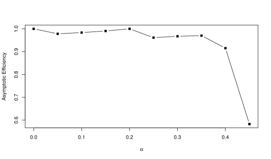
Figure 1: The asymptotic efficiency of $\hat{g}_{n,\alpha}(x_{0})$ relative to $\hat{g}_{n,NW}(x_{0})$ plotted for different values of $\alpha$ when $x_{0}=0.50$, and $X$ follows uniform distribution over $(0,1)$.

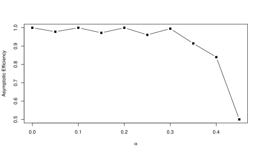
Figure 2: The asymptotic efficiency of $\hat{g}_{n,\alpha}(x_{0})$ relative to $\hat{g}_{n,NW}(x_{0})$ plotted for different values of $\alpha$ when $x_{0}=0.50$, and $X$ follows beta distribution with the scale parameter $=2$ and the shape parameter $=2$.

4 Breakdown Point

In the earlier section, we established the asymptotic distribution of $\hat{g}_{n,\alpha}(x_{0})$ and studied its asymptotic efficiency for various choices of $\alpha$ and $x_{0}$. Also, it was mentioned that there is a trade-off between the efficiency and the robustness of an estimator. To explore the issue of the robustness of $\hat{g}_{n,\alpha}(x_{0})$, we here study the finite sample breakdown point (see, e.g., rousseeuw2005robust) of $\hat{g}_{n,\alpha}(x_{0})$.

For sake of completeness, we here define the finite sample breakdown point of an estimator $T$. The maximum bias of $T$ with respect to a sample $\mathcal{X}=\{X_{1},\ldots,X_{n}\}$ $(X_{i}\in\mathbb{R}^{d},d\geqslant 1,i=1,\ldots,n)$ is defined as $\displaystyle b\left(m,T,\mathcal{X}\right)=\sup_{\mathcal{X}^{\prime}}|T(\mathcal{X}^{\prime})-T(\mathcal{X})|$, where $\mathcal{X}^{\prime}$ is the corrupted sample obtained by replacing $m$ sample points from $\mathcal{X}$. Finally, the breakdown point of $T$ is defined as

$$\epsilon^{\star}_{n}\left(T,\mathcal{X}\right)=\inf_{m}\left\{\frac{m}{n}\,\Big{|}\,b\left(m,T,\mathcal{X}\right)\text{ is unbounded}\right\}.$$

To compute the breakdown point of $\hat{g}_{n,\alpha}(x_{0})$, one needs to assume the following conditions.

(B1) The kernel $K(\cdot)$ is a bounded probability density function with support $(-\tau,\tau)$, where $\tau>0$.

(B2) $\displaystyle\int_{-\tau}^{\tau}K(u)du=1$.

(B3) $\displaystyle h_{n}^{-1}K\left(h_{n}^{-1}\right)=O(1)$.

The following theorem describes the breakdown point of $\hat{g}_{n,\alpha}(\cdot)$.

Theorem 4.1.

Under the assumptions (B1), (B2) and (B3), for any $\alpha\in[0,\frac{1}{2})$, the finite sample breakdown point of $\hat{g}_{n,\alpha}(\cdot)$ is $\epsilon^{\star}_{n}\left(\hat{g}_{n,\alpha}(x_{0}),\mathcal{X}\right)$ = $\displaystyle\frac{[n\alpha]}{n}$, and consequently, the asymptotic breakdown point is $\epsilon^{\star}\left(\hat{g}_{n,\alpha}(x_{0}),\mathcal{X}\right)=\displaystyle\lim_{n\rightarrow\infty}\epsilon^{\star}_{n}\left(\hat{g}_{n,\alpha}(x_{0}),\mathcal{X}\right)=\alpha$.

Proof.

Let $\mathcal{X}=\{(X_{1},Y_{1}),\ldots,(X_{n},Y_{n})\}$, then $\hat{g}_{n,\alpha}(x_{0})$ based on $\mathcal{X}$ as follows:

$$\hat{g}_{n,\alpha}(x_{0})=\frac{\sum\limits_{i=[n\alpha]+1}^{n-[n\alpha]}k_{n}\left(X_{(i)}-x_{0}\right)Y_{[i]}}{\sum\limits_{i=[n\alpha]+1}^{n-[n\alpha]}k_{n}\left(X_{(i)}-x_{0}\right)}=\frac{(n-2[n\alpha])^{-1}\sum\limits_{i=[n\alpha]+1}^{n-[n\alpha]}k_{n}\left(X_{(i)}-x_{0}\right)Y_{[i]}}{(n-2[n\alpha])^{-1}\sum\limits_{i=[n\alpha]+1}^{n-[n\alpha]}k_{n}\left(X_{(i)}-x_{0}\right)}.$$

The minimum bias of $\hat{g}_{n,\alpha}(x_{0})$ is then expressed as $\displaystyle b\left(m,\hat{g}_{n,\alpha}(x_{0}),\mathcal{X}\right)=\sup_{\mathcal{X}^{\prime}}\left\lVert\hat{g}_{n,\alpha}(x_{0})(\mathcal{X}^{\prime})-\hat{g}_{n,\alpha}(x_{0})(\mathcal{X})\right\rVert$.

Let us first consider $m=[n\alpha]$, and after replacing $m$ pairs of $(X_{i},Y_{i})$ with arbitrarily large values $(X_{i}^{\prime},Y_{i}^{\prime})$, the estimator remains unchanged. The reason is as follows: for all contaminated pairs $(X_{i}^{\prime},Y_{i}^{\prime})$, we have $(X_{i}^{\prime},Y_{i}^{\prime})=(X_{(j)},Y_{[j]})$ for some $j>n-[n\alpha]$. This fact implies that $\hat{g}_{n,\alpha}(x)(\mathcal{X}^{\prime})=\hat{g}_{n,\alpha}(x_{0})(\mathcal{X})$ when $[n\alpha]$ number of observations are contaminated. Hence, $\displaystyle b\left([n\alpha],\hat{g}_{n,\alpha}(x_{0}),\mathcal{X}\right)=0$, and consequently,

$$\epsilon^{\star}_{n}\left(\hat{g}_{n,\alpha}(x_{0}),\mathcal{X}\right)\geqslant\frac{[n\alpha]}{n}.$$ (6)

For the reverse inequality, suppose that $m=[n\alpha]+1$ many observations (denoted as $(X_{i}^{\prime},Y_{i}^{\prime})$) are corrupted. Note that under this circumstance, for at least one value of $i\in\{1,\ldots,n\}$, $(X_{i}^{\prime},Y_{i}^{\prime})=(X_{(j)},Y_{[j]})$ for some $j\leqslant n-[n\alpha]$. Now, the denominator of $\hat{g}_{n,\alpha}(x_{0})$ is bounded, i.e., $\displaystyle(n-2[n\alpha])^{-1}\sum\limits_{i=[n\alpha]+1}^{n-[n\alpha]}k_{n}\left(X_{(i)}-x_{0}\right)<\infty$ for all $x_{0}$ (using (B3)), and the numerator of $\hat{g}_{n,\alpha}(x_{0})(\mathcal{X}^{\prime})$ is unbounded, since the sum $\displaystyle(n-2[n\alpha])^{-1}\sum\limits_{i=[n\alpha]+1}^{n-[n\alpha]}k_{n}\left(X_{(i)}-x_{0}\right)Y_{[i]}$ has at least one contaminated $Y_{[i]}$, which makes $\hat{g}_{n,\alpha}(x_{0})$ unbounded. Therefore, $b\left([n\alpha]+1,\hat{g}_{n,\alpha}(x_{0}),\mathcal{X}\right)$ becomes unbounded, and hence,

$$\epsilon^{\star}_{n}\left(\hat{g}_{n,\alpha}(x_{0}),\mathcal{X}\right)<\frac{[n\alpha]+1}{n}.$$ (7)

Combining (6) and (7), we have $\displaystyle\epsilon^{\star}_{n}\left(\hat{g}_{n,\alpha}(x_{0}),\mathcal{X}\right)=\frac{[n\alpha]}{n}$. Consequently, the asymptotic breakdown point is $\epsilon^{\star}\left(\hat{g}_{n,\alpha}(x_{0}),\mathcal{X}\right)=\displaystyle\lim_{n\rightarrow\infty}\epsilon^{\star}_{n}\left(\hat{g}_{n,\alpha}(x_{0}),\mathcal{X}\right)=\alpha$. ∎

The assertion in Theorem 4.1 indicates that the asymptotic breakdown point of $\hat{g}_{n,\alpha}(x_{0})$ is $\alpha$ for any $x_{0}$, which further implies that it attains the highest asymptotic breakdown point $\frac{1}{2}$ when the trimming proportion $\alpha\rightarrow\frac{1}{2}$. On the other hand, when $\alpha=0$, the asymptotic breakdown point will be the lowest possible value zero, which is a formal reason why usual Nadarya-Watson estimator, i.e., $\hat{g}_{n,NW}(.)$ is a non-robust estimator. Overall, the fact is that the robustness of the estimator $\hat{g}_{n,\alpha}(\cdot)$ will increase as the trimming proportion increases unlike the case of efficiency study. In fact, as it is mentioned earlier, this is the reason why the choice of trimming proportion in $\hat{g}_{n,\alpha}$ is an issue of concern as $\alpha$ controls the both the efficiency and the robustness properties of the estimator. Moreover, since the efficiency of the estimator depends on the sample size $n$ as well, we study the finite sample efficiency of the estimator in the next section.

5 Finite Sample Study

In Section 3.1, we studied the efficiency of $\hat{g}_{n,\alpha}(x_{0})$ for various choices of $\alpha$ and $x_{0}$ when the sample size tends to infinity, and it showed various features in the performance of $\hat{g}_{n,\alpha}(x_{0})$ in terms of the asymptotic efficiency. We are now interested to see the performance of $\hat{g}_{n,\alpha}(x_{0})$ for different values of $\alpha$ when the sample size is finite. In the numerical study, we consider $\alpha=0.05,0.10,\ldots,0.45$ and $n=50$ and $500$. Here also, Epanechnikov Kernel (see, e.g., silverman1986density) is used with $h_{n}=\frac{n^{-\frac{1}{2}}}{2}$, and the co-variates are generated from uniform distribution over $(0,1)$, unless mentioned otherwise. We study both linear and non linear model coupled with standard normal and $t$-distribution with 5 degrees of freedom as the distribution of the error random variables. All results are summarized in Figures 3, 4, 5 and 6, and in the tabular form in Appendix B.

We compute the finite sample efficiency as follows: Using the form of the model and the distribution of the error random variable, we generate $(x_{1,j},y_{1,j}),\ldots,(x_{n,j},y_{n,j})$, when $j=1,\ldots,N$. Afterwards, for each $j=1,\ldots,N$, we compute $\hat{g}_{n,\alpha}(x_{0})$ for different values of $\alpha$ and $\hat{g}_{n,NW}(x_{0})$ as well. Let the values of $\hat{g}_{n,\alpha}(x_{0})$ and $\hat{g}_{n,NW}(x_{0})$ be $(U_{1},\ldots,U_{N})$ and $(V_{1},\ldots,V_{N})$, respectively, and finally, the finite sample efficiency of $\hat{g}_{n,\alpha}(x_{0})$ relative to $\hat{g}_{n,NW}(x_{0})$ is defined as $\frac{\frac{1}{N}\sum\limits_{i=1}^{N}\left(V_{i}-\frac{1}{N}\sum\limits_{i=1}^{N}V_{i}\right)^{2}}{\frac{1}{N}\sum\limits_{i=1}^{N}\left(U_{i}-\frac{1}{N}\sum\limits_{i=1}^{N}U_{i}\right)^{2}}$. In the numerical study, we consider $N=1000$ and $x_{0}=0.50$. In Figures 3, 4, 5 and 6, we plot the finite sample efficiency of $\hat{g}_{n,\alpha}$ relative to $\hat{g}_{n,NW}$ for different values of $\alpha$, for four different underlying model.

Example 1: Model: $Y=5X+e$, where $e$ follows standard normal distribution.

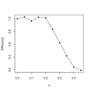
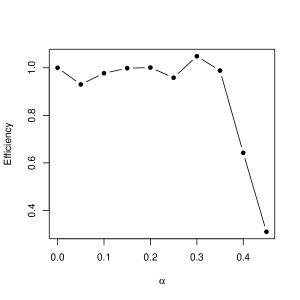
Figure 3: For different values of $\alpha$, the finite sample efficiency of $\hat{g}_{n,\alpha}(0.5)$ relative to $\hat{g}_{n,NW}(0.5)$ for Example 1. The left diagram is for $n=50$, and the right diagram is for $n=500$.

The diagrams in Figures 3, 4, 5 and 6 indicate that $\hat{g}_{n,\alpha}(x_{0})$ has good efficiency relative to $\hat{g}_{n,NW}(x_{0})$ for a wide range of $\alpha$ regardless of the choice of the model and/or the choice of the distribution of the error random variable.

Example 2: Model: $Y=4X^{3}+e$, where $e$ follows standard normal distribution.

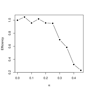
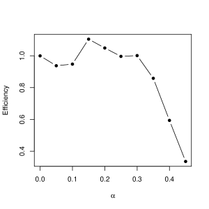
Figure 4: For different values of $\alpha$, the finite sample efficiency of $\hat{g}_{n,\alpha}(0.5)$ relative to $\hat{g}_{n,NW}(0.5)$ for Example 2. The left diagram is for $n=50$, and the right diagram is for $n=500$.

Example 3: Model: $Y=5X+e$, where $e$ follows $t$-distribution with $5$ degrees of freedom.

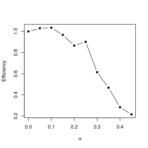
Figure 5: For different values of $\alpha$, the finite sample efficiency of $\hat{g}_{n,\alpha}(0.5)$ relative to $\hat{g}_{n,NW}(0.5)$ for Example 3. The left diagram is for $n=50$, and the right diagram is for $n=500$.

Example 4: Model: $Y=4X^{3}+e$, where $e$ follows $t$-distribution with $5$ degrees of freedom.

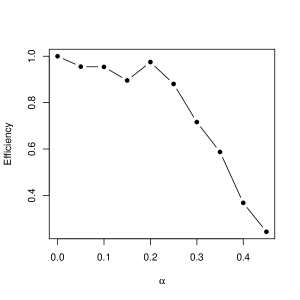
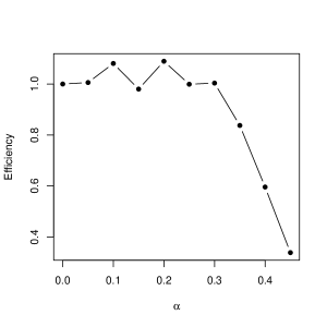
Figure 6: For different values of $\alpha$, the finite sample efficiency of $\hat{g}_{n,\alpha}(0.5)$ relative to $\hat{g}_{n,NW}(0.5)$ for Example 4. The left diagram is for $n=50$, and the right diagram is for $n=500$.

6 Real Data Analysis

In this section, we illustrate the functionality of our proposed estimator on some benchmark real data sets. All these data sets are available in UCI machine repository.

Combined Cycle Power Plant Data Set: This data set contains 9568 data points collected from a Combined Cycle Power Plant over six years (2006-2011), when the plant was set to work with full load (see kaya2012local and tufekci2014prediction for details). The data set can be accessed with the following link: https://archive.ics.uci.edu/ml/datasets/Combined+Cycle+Power+Plant. The data contains five attributes: Temperature (in ^∘C), Ambient Pressure (in milibar), Relative Humidity (in %), Exhaust Vacuum (in cm Hg) and Electrical Energy Output (in MW). We consider Temperature as our co-variate or independent variable ($X$) and Electrical Energy output as response or dependent variable ($Y$). We provide a scatter plot of the Electrical Energy Output against Temperature in the first diagram of Figure 7.

In the study, we first scaled the data associated with the co-variate to the interval $[0,1]$ using the transformation $x^{*}=\frac{x-\min(x)}{\max(x)-\min(x)}$, where $x^{*}$ is the transformed variable, and we adopt Bootstrap methodology to compute the efficiency, which is called as Bootstrap efficiency. The procedure : We first generate $B$ many Bootstrap resamples with size $n$ from the data $(y_{1},x_{1}^{*}),\ldots,(y_{n},x_{n}^{*})$, and compute the values of $\hat{g}_{n,\alpha}(x_{0})$ and $\hat{g}_{n,NW}(x_{0})$ for each resample. Let us denote those values of $\hat{g}_{n,\alpha}(x_{0})$ and $\hat{g}_{n,NW}(x_{0})$ as $(S_{1},\ldots,S_{B})$ and $(R_{1},\ldots,R_{B})$, respectively. Then the Bootstrap efficiency of $\hat{g}_{n,\alpha}(x_{0})$ relative to $\hat{g}_{n,NW}(x_{0})$ is defined as $\frac{\frac{1}{B}\sum\limits_{i=1}^{B}\left(R_{i}-\frac{1}{B}\sum\limits_{i=1}^{B}R_{i}\right)^{2}}{\frac{1}{B}\sum\limits_{i=1}^{B}\left(S_{i}-\frac{1}{B}\sum\limits_{i=1}^{B}S_{i}\right)^{2}}.$ In the second diagram of Figure 7, we plot the Bootstrap efficiency of $\hat{g}_{n,\alpha}(x_{0})$ relative to $\hat{g}_{n,NW}(x_{0})$ for different values of $\alpha$ for this data (here $n=9568$). In this study, we consider Epanechnikov kernel with bandwidth $h_{n}=\frac{n^{-\frac{1}{2}}}{2}$ and $B=1000$. The second diagram of Figure 7 indicates that the efficiency of $\hat{g}_{n,\alpha}$ relative to $\hat{g}_{n,NW}$ is substantially high for a wide range of $\alpha$, and the most probable reason is that the data has a few influential observations.

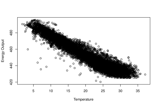
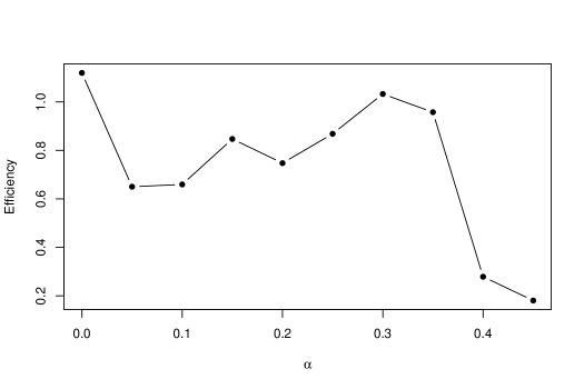
Figure 7: Scatter plot (Up) of the Combined Cycle Power Plant Data and Efficiency (Down) of $\hat{g}_{n,\alpha}(x_{0})$ relative to $\hat{g}_{n,NW}(x_{0})$ at $x_{0}=0.50$ plotted for different values of $\alpha$.

Parkinson’s Telemonitoring Data Set: This data set consists of 5875 recordings of several medical voice measures from forty two people with early-stage Parkinson’s disease recruited to a six month trial of a telemonitoring device, for remote symptom progression monitoring (see tsanas2009accurate for details). This data can be accessed with the following link: https://archive.ics.uci.edu/ml/datasets/Parkinsons+Telemonitoring. The data has 22 attributes, out of which two attributes are of our interest for this study: NHR (measure of ratio of noise to tonal components in the voice) and RPDE (A nonlinear dynamical complexity measure). We consider the attribute NHR as our co-variate or independent variable ($X$) and RPDE as our response or dependent variable ($Y$). We provide a scatter plot of RPDE against NHR variable in the first diagram of Figure 8. Unlike the earlier data analysis, the transformation of the co-variate has not been done here as the values of NHR variable belongs to $[0,1]$.

Here also, we compute the Bootstrap efficiency $\hat{g}_{n,\alpha}(x_{0})$ relative to $\hat{g}_{n,NW}(x_{0})$ based on the data $(Y,X)$, and the procedure is same as it is described in the earlier real data analysis. In the second diagram of Figure 8, we plot the Bootstrap efficiency of $\hat{g}_{n,\alpha}(x_{0})$ relative to $\hat{g}_{n,NW}(x_{0})$ for different values of $\alpha$ for this data (here $n=5875$). In this study also, we consider Epanechnikov kernel with bandwidth $h_{n}=\frac{n^{-\frac{1}{2}}}{2}$ and $B=1000$. Here also, the second diagram of Figure 7 indicates the efficiency of $\hat{g}_{n,\alpha}$ relative to $\hat{g}_{n,NW}$ is substantially high for a wide range of $\alpha$, and as we indicated in the earlier study, the most probable reason is that the data has a few influential observations.

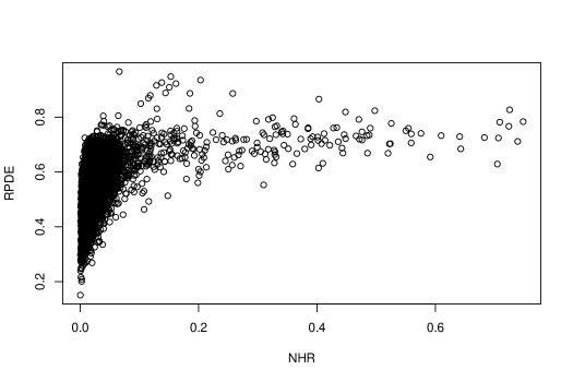
Figure 8: Scatter plot (Up) of the Parkinson’s Telemonitoring Data and Efficiency (Down) of $\hat{g}_{n,\alpha}(x_{0})$ relative to $\hat{g}_{n,NW}(x_{0})$ at $x_{0}=0.50$ plotted for different values of $\alpha$.

Air Quality Data Set: This data set contains 9358 instances of hourly averaged responses from an array of five metal oxide chemical sensors embedded in an Air Quality Chemical Multisensor Device (see de2008field for details). The device was set up in a polluted area of an Italian city, at road level. The data set can be accessed with the following link: https://archive.ics.uci.edu/ml/datasets/Air+quality. There are thirteen attributes in this data apart from date and time:
1 True hourly averaged concentration $CO$ in $mg/m^{3}$ (reference analyzer).
2 PT08.S1 (tin oxide) hourly averaged sensor response (nominally CO targeted).
3 True hourly averaged overall Non Metanic Hydrocarbons concentration in $microg/m^{3}$ (reference analyzer).
4 True hourly averaged Benzene concentration in $microg/m^{3}$ (reference analyzer).
5 PT08.S2 (titania) hourly averaged sensor response (nominally NMHC targeted).
6 True hourly averaged NOx concentration in ppb (reference analyzer).
7 PT08.S3 (tungsten oxide) hourly averaged sensor response (nominally NOx targeted).
8 True hourly averaged NO2 concentration in $microg/m^{3}$ (reference analyzer).
9 PT08.S4 (tungsten oxide) hourly averaged sensor response (nominally NO2 targeted).
10 PT08.S5 (indium oxide) hourly averaged sensor response (nominally O3 targeted).
11 Temperature in ^∘C.
12 Relative Humidity (%).
13 AH: Absolute Humidity.
We consider the quantity of Tungsten Oxide as the co-variate or the independent variable ($X$), and the Absolute Humidity is considered as the response or dependent variable ($Y$). We provide a scatter plot of Absolute Humidity against Tungsten Oxide in the first diagram of Figure 9, and the scatter plot indicates that the data does not have as such any influential or outlier observations.

In the study, as we did for the first real data analysis, the co-variate is scaled to the interval $[0,1]$ using the transformation $x^{*}=\frac{x-\min(x)}{\max(x)-\min(x)}$, where $x^{*}$ is the transformed variable, and we here also adopt Bootstrap methodology to compute the efficiency. The computational procedure of the Bootstrap efficiency is same as we described in the first real data analysis. In the second diagram of Figure 9, we plot the Bootstrap efficiency of $\hat{g}_{n,\alpha}(x_{0})$ relative to $\hat{g}_{n,NW}(x_{0})$ for different values of $\alpha$ for this data (here $n=9358$). In this study also, we consider Epanechnikov kernel with bandwidth $h_{n}=\frac{n^{-\frac{1}{2}}}{2}$ and $B=1000$. The second diagram of Figure 9 indicates the efficiency of $\hat{g}_{n,\alpha}$ relative to $\hat{g}_{n,NW}$ is high for small values $\alpha$, and decreases gradually as $\alpha$ increases. It is expected since the data does not have any substantial outliers, $\hat{g}_{n,\alpha}(x_{0})$ performs well for small values of $\alpha$, i.e., when $\hat{g}_{n,\alpha}$ is almost same as $\hat{g}_{n,NW}$. On the other hand, the efficiency of $\hat{g}_{n,\alpha}$ steadily goes down for larger values of $\alpha$ as $\hat{g}_{n,\alpha}$ is different from $\hat{g}_{n,NW}$ by a great amount when $\alpha$ is large.

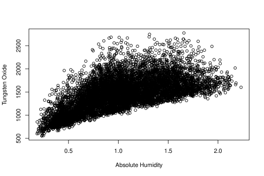
Figure 9: Scatter plot (Up) of the Air Quality Data and Efficiency (Down) of $\hat{g}_{n,\alpha}(x_{0})$ relative to $\hat{g}_{n,NW}(x_{0})$ at $x_{0}=0.50$ plotted for different values of $\alpha$.

7 Concluding Remarks

Local linear or local polynomial version:

The estimator studied in this article is a local constant trimmed mean for the non-parametric regression function (see (3)). Following the same spirit of (3), one can define a local linear or even local polynomial version of the trimmed mean for non-parametric regression function. However, at the same time, adding more variables may create various problems associated with the issue of variable selection. Choosing appropriate degree of polynomial version of the trimmed mean may be an interest of future research. Besides, one of the well-known problem of using the local constant estimator is the adverse effect of boundary (see e.g., fan1996local). However, since the trimming based estimator is based on the ordered observations and the procedure of trimming, the proposed estimator can avoid the negative effect of boundary.

Uniform convergence and influence function:

In Theorem 3.1, we stated the pointwise weak convergence of $\hat{g}_{n,\alpha}(x)$, and it is indeed true that the result would be more appealing if one can establish the process convergence of $\hat{g}_{n,\alpha}(x)$, which allows us to study the related testing of hypothesis problem based on $\hat{g}_{n,\alpha}(x)$. However, to prove the process convergence of $\hat{g}_{n,\alpha}(x)$, one needs to establish the tightness property of $\hat{g}_{n,\alpha}(x)$, which is not easily doable. Regarding the robustness property of $\hat{g}_{n,\alpha}(x)$, along with the breakdown point, one may also consider the gross error sensitivity (see huber1981robust, p.14) as a measure of robustness. However, since the gross error sensitivity only measures the local robustness of an estimator whereas the breakdown point measures the global robustness of the estimator, we here investigate the breakdown point of the proposed estimator.

The choice of kernel function and bandwidth:

The choice of kernel function along with its bandwidth another issue of concern. In our numerical study, we consider Epanechnikov kernel since it is the most efficient kernel among the symmetric kernel (see silverman1986density, p.59). Regarding the choice of bandwidth, we consider $h_{n}=\frac{n^{-\frac{1}{2}}}{2}$ since it satisfies $h_{n}\rightarrow 0$ and $nh_{n}\rightarrow\infty$ as $n\rightarrow\infty$. However, since the aforesaid criterion is asymptotic in nature, one can adopt the methodology based on data driven approach but using such choice of bandwidth, deriving the asymptotic distribution of the proposed estimator will become more challenging.

Main contribution of this article:

In this article, we propose a new estimator for the non-parametric regression function, which coincides with the well-known Nadarya-Watson estimator as a special case. The characterization of the proposed estimator through an optimization problem is also discussed. In the study, we have observed that the proposed estimator can maintain a good efficiency with high break down point for a wide range of trimming proportion, which is a rare attribute of any estimator. The estimator performs well on real data as well.

8 Appendix

8.1 Appendix A : Proofs

We first present a fact, which is used to compute the asymptotic efficiency of $\hat{g}_{n,\alpha}(x_{0})$ relative to $\hat{g}_{n,NW}(x_{0})$ in Section 3.1.

Fact A: Let $X_{(i)}$ be the $i$-th order statistic of the i.i.d. random variables $\{X_{1},\ldots,X_{n}\}$ with common density $f_{X}$ and distribution function $F_{X}$. Suppose that $f_{X_{(i)}}$ is the probability density function of $X_{(i)}$ for $i=1,\ldots,n$. Then for any $x_{0}$,

$$\frac{1}{n}\sum_{i=1}^{n}f_{X_{(i)}}(x_{0})=f_{X}(x_{0}).$$

Proof of Fact A: Note that for any arbitrary $x_{0}$, and $i=1,\ldots,n$, we have

$$f_{X_{(i)}}(x_{0})=\frac{n!}{(i-1)!(n-i)!}[F_{X}(x_{0})]^{i-1}[1-F_{X}(x_{0})]^{n-i}f_{X}(x_{0}).$$

Now, taking sum over $i$, we have

$$\begin{split}\sum_{i=1}^{n}f_{X_{(i)}}(x_{0})&=\sum_{i=1}^{n}\frac{n!}{(i-1)!(n-i)!}[F_{X}(x_{0})]^{i-1}[1-F_{X}(x_{0})]^{n-i}f_{X}(x_{0})\\ &=n\sum_{i=1}^{n}\frac{(n-1)!}{(i-1)!(n-i)!}[F_{X}(x_{0})]^{i-1}[1-F_{X}(x_{0})]^{n-i}f_{X}(x_{0})\\ &=n[F_{X}(x_{0})+1-F_{X}(x_{0})]^{n-1}f_{X}(x_{0})=nf_{X}(x_{0}).\end{split}$$

Hence, $\frac{1}{n}\sum_{i=1}^{n}f_{X_{(i)}}(x_{0})=f_{X}(x_{0})$ for any arbitrary $x_{0}$, which completes the proof. $\Box$

Fact B:

$$AE(\hat{g}_{n,\alpha}(x),\hat{g}_{n,NW}(x))=\frac{(1-2\alpha)t_{\alpha}(x)}{f_{X}(x)}\leq 1$$

for any $x$ and $\alpha\in[0,\frac{1}{2})$. Here the notations are same as defined in Section 3.1.

Proof of Fact B: Using the form of the probability density function of $X_{(i)}$, we have

$$\begin{split}t_{\alpha}(x)=\frac{1}{(n-2[n\alpha])}\sum\limits_{i=[n\alpha]+1}^{n-[n\alpha]}f_{X_{(i)}}(x)&=\frac{1}{(n-2[n\alpha])}\sum\limits_{i=[n\alpha]+1}^{n-[n\alpha]}nC(n-1,i-1)[F_{X}(x)]^{i-1}[1-F_{X}(x)]^{n-i}f_{X}(x)\\ &=\frac{nf_{X}(x)}{(n-2[n\alpha])}\sum\limits_{i=[n\alpha]+1}^{n-[n\alpha]}C(n-1,i-1)[F_{X}(x)]^{i-1}[1-F_{X}(x)]^{n-i},\end{split}$$ (8)

where $F_{X}$ is the distribution function of $X$ and $C(n-1,i-1)=\frac{(n-1)!}{(i-1)!(n-i)!}$. We also note that,

$$\sum\limits_{i=[n\alpha]+1}^{n-[n\alpha]}C(n-1,i-1)[F_{X}(x)]^{i-1}[1-F_{X}(x)]^{n-i}\leqslant\sum\limits_{i=1}^{n}C(n-1,i-1)[F_{X}(x)]^{i-1}[1-F_{X}(x)]^{n-i}=1,$$ (9)

for all $n$ and any fixed $\alpha\in[0,\frac{1}{2})$. Hence, (8) and (9) together give us

$$t_{\alpha}(x)=\lim_{n\to\infty}\frac{1}{(n-2[n\alpha])}\sum\limits_{i=[n\alpha]+1}^{n-[n\alpha]}f_{X_{(i)}}(x)\leqslant\lim_{n\to\infty}\frac{nf_{X}(x)}{(n-2[n\alpha])}=\frac{f_{X}(x)}{(1-2\alpha)}.$$

It completes the proof. $\Box$

In order to prove Theorem 3.1, one needs the following lemmas.

Lemma 8.1.

Let $\displaystyle\hat{f}_{n,\alpha}(x_{0})=\frac{1}{(n-2[n\alpha])h_{n}}\sum\limits_{i=[n\alpha]+1}^{n-[n\alpha]}K\left(\frac{X_{(i)}-x_{0}}{h_{n}}\right)$, where $K$ is the kernel function. Then, under (A1)-(A5), for any arbitrary $x_{0}$, $\displaystyle\hat{f}_{n,\alpha}(x_{0})\xrightarrow{\makebox[14.22636pt]{p}}\lim_{n\to\infty}\frac{1}{(n-2[n\alpha])}\sum\limits_{i=[n\alpha]+1}^{n-[n\alpha]}f_{X_{(i)}}(x_{0})$ as $n\to\infty$, where $f_{X_{(i)}}(\cdot)$ is the density function of $i$-th order statistic $X_{(i)}$.

Proof.

To prove this lemma, it is enough to show that for any arbitrary $x_{0}$, $E[\hat{f}_{n,\alpha}(x_{0})]\rightarrow\displaystyle\lim_{n\rightarrow\infty}\frac{1}{(n-2[n\alpha])}\sum\limits_{i=[n\alpha]+1}^{n-[n\alpha]}f_{X_{i}}(x_{0})$ as $n\rightarrow\infty$ and variance$[\hat{f}_{n,\alpha}(x_{0})]\rightarrow 0$ as $n\rightarrow\infty$.

We now consider

$$\begin{split}E\left(\hat{f}_{n,\alpha}(x_{0})\right)&=\frac{1}{h_{n}(n-2[n\alpha])}\sum\limits_{i=[n\alpha]+1}^{n-[n\alpha]}E\left[K\left(\frac{X_{(i)}-x_{0}}{h_{n}}\right)\right]\\ &=\frac{1}{h_{n}(n-2[n\alpha])}\sum\limits_{i=[n\alpha]+1}^{n-[n\alpha]}\int K\left(\frac{u-x_{0}}{h_{n}}\right)f_{X_{(i)}}(u)du\end{split}$$

Using $\displaystyle\frac{u-x_{0}}{h_{n}}=z$ yields

$$\begin{split}E\left(\hat{f}_{n,\alpha}(x_{0})\right)&=\frac{1}{h_{n}(n-2[n\alpha])}\sum\limits_{i=[n\alpha]+1}^{n-[n\alpha]}h_{n}\int K(z)f_{X_{(i)}}(x_{0}+h_{n}z)dz\\ &=\frac{1}{(n-2[n\alpha])}\sum\limits_{i=[n\alpha]+1}^{n-[n\alpha]}\int K(z)f_{X_{(i)}}(x_{0}+h_{n}z)dz\\ &\to\lim_{n\to\infty}\frac{1}{(n-2[n\alpha])}\sum\limits_{i=[n\alpha]+1}^{n-[n\alpha]}f_{X_{(i)}}(x_{0})\end{split}$$

as $n\to\infty$, for each $x_{0}$. The last implication follows from the application of dominated convergence theorem using the facts that $f_{X_{(i)}}$ is a bounded function (follows from (A2)), $h_{n}\rightarrow 0$ as $n\rightarrow\infty$ and $\int\limits_{-\tau}^{\tau}k(z)dz=1$.

Next, consider ($var$ denotes the variance and $cov$ denotes the co-variance)

$$\begin{split}var\left(\hat{f}_{n,\alpha}(x_{0})\right)&=\frac{1}{h_{n}^{2}(n-2[n\alpha])^{2}}\sum\limits_{i=[n\alpha]+1}^{n-[n\alpha]}var\left[K\left(\frac{X_{(i)}-x_{0}}{h_{n}}\right)\right]\\ &+\frac{1}{h_{n}^{2}(n-2[n\alpha])^{2}}\sum\limits_{i\neq j=[n\alpha]+1}^{n-[n\alpha]}cov\left[K\left(\frac{X_{(i)}-x_{0}}{h_{n}}\right),K\left(\frac{X_{(j)}-x_{0}}{h_{n}}\right)\right]\\ &=\frac{1}{h_{n}^{2}(n-2[n\alpha])^{2}}\sum\limits_{i=[n\alpha]+1}^{n-[n\alpha]}E\left[K\left(\frac{X_{(i)}-x_{0}}{h_{n}}\right)^{2}\right]-E\left[\left\{K\left(\frac{X_{(i)}-x_{0}}{h_{n}}\right)\right\}\right]^{2}\\ &+\frac{1}{h_{n}^{2}(n-2[n\alpha])^{2}}\sum\limits_{i\neq j=[n\alpha]+1}^{n-[n\alpha]}cov\left[K\left(\frac{X_{(i)}-x_{0}}{h_{n}}\right),K\left(\frac{X_{(j)}-x_{0}}{h_{n}}\right)\right]\\ &=\frac{1}{h_{n}^{2}(n-2[n\alpha])^{2}}\sum\limits_{i=[n\alpha]+1}^{n-[n\alpha]}\int\left[K\left(\frac{u-x_{0}}{h_{n}}\right)\right]^{2}f_{X_{(i)}}(u)du\\ &-\frac{1}{h_{n}^{2}(n-2[n\alpha])^{2}}\sum\limits_{i=[n\alpha]+1}^{n-[n\alpha]}\left(\int K\left(\frac{u-x_{0}}{h_{n}}\right)f_{X_{(i)}}(u)du\right)^{2}\\ &+\frac{1}{h_{n}^{2}(n-2[n\alpha])^{2}}\sum\limits_{i\neq j=[n\alpha]+1}^{n-[n\alpha]}cov\left[K\left(\frac{X_{(i)}-x_{0}}{h_{n}}\right),K\left(\frac{X_{(j)}-x_{0}}{h_{n}}\right)\right].\end{split}$$ (10)

Note that since for any random variable Y, $var(Y)\leq E[Y^{2}]$ and $var(Y)\geq 0$ along with the fact that for any two random variables $X$ and $Y$, $|cov(X,Y)|\leq\sqrt{var(X)var(Y)}$, it is now enough to show that $\frac{1}{h_{n}^{2}(n-2[n\alpha])^{2}}\sum\limits_{i=[n\alpha]+1}^{n-[n\alpha]}\int\left[K\left(\frac{u-x_{0}}{h_{n}}\right)\right]^{2}f_{X_{(i)}}(u)du\rightarrow 0$ as $n\rightarrow\infty$. Using the transformation $\displaystyle z=\frac{u-x_{0}}{h_{n}}$, we have

$$\begin{split}\frac{1}{h_{n}^{2}(n-2[n\alpha])^{2}}&\sum\limits_{i=[n\alpha]+1}^{n-[n\alpha]}\int\left[K\left(\frac{u-x_{0}}{h_{n}}\right)\right]^{2}f_{X_{(i)}}(u)du\\ &=\frac{1}{h_{n}^{2}(n-2[n\alpha])^{2}}\sum\limits_{i=[n\alpha]+1}^{n-[n\alpha]}h_{n}\int\{K(z)\}^{2}f_{X_{(i)}}(x_{0}+h_{n}z)dz\\ &=\frac{1}{h_{n}(n-2[n\alpha])}\frac{1}{(n-2[n\alpha])}\sum\limits_{i=[n\alpha]+1}^{n-[n\alpha]}\int\{K(z)\}^{2}f_{X_{(i)}}(x_{0}+h_{n}z)dz.\end{split}$$

Here since $nh_{n}\rightarrow\infty$ as $n\rightarrow\infty$, $\displaystyle\lim_{n\to\infty}h_{n}^{-1}(n-2[n\alpha])^{-1}=0$ for a fixed $\alpha\in[0,\frac{1}{2})$, we have

$$\frac{1}{(n-2[n\alpha])}\sum\limits_{i=[n\alpha]+1}^{n-[n\alpha]}\int\{K(z)\}^{2}f_{X_{(i)}}(x_{0}+h_{n}z)dz\to\lim_{n\to\infty}\frac{1}{(n-2[n\alpha])}\sum\limits_{i=[n\alpha]+1}^{n-[n\alpha]}f_{X_{i}}(x_{0})$$

as $n\to\infty$ for each $x_{0}$ using the same argument provided for $E[\hat{f}_{n,\alpha}(x_{0})]$. Thus

$$\frac{1}{h_{n}^{2}(n-2[n\alpha])^{2}}\sum\limits_{i=[n\alpha]+1}^{n-[n\alpha]}\int K\left(\frac{u-x_{0}}{h_{n}}\right)^{2}f_{X_{i}}(u)du\to 0$$

as $n\to\infty$, and hence, $var\left(\hat{f}_{n,\alpha}(x_{0})\right)\rightarrow 0$ as $n\rightarrow\infty$. It completes the proof.

∎

Lemma 8.2.

Let

$$\hat{m}_{1,n}(x_{0})=\frac{1}{(n-2[n\alpha])h_{n}}\sum\limits_{i=[n\alpha]+1}^{n-[n\alpha]}K\left(\frac{X_{(i)}-x_{0}}{h_{n}}\right)\left(g(X_{(i)})-g(x_{0})\right),$$ (11)

where $K$ is the kernel function, $g$ is the regression function and $X_{(i)}$ is the $i$-th order statistic. Then under (A1)-(A5), we have

$$E(\hat{m}_{1,n}(x_{0}))=\frac{h_{n}^{2}g^{\prime\prime}(x_{0})\,k_{2}}{2\left(n-2[n\alpha]\right)}\sum\limits_{i=[n\alpha]+1}^{n-[n\alpha]}f_{X_{(i)}}(x_{0})+\frac{h_{n}^{2}g^{\prime}(x_{0})\,k_{2}}{\left(n-2[n\alpha]\right)}\sum\limits_{i=[n\alpha]+1}^{n-[n\alpha]}f^{\prime}_{X_{(i)}}(x_{0})+o(h_{n}^{2})$$

for each $x_{0}$, where $g^{\prime}$ and $g^{\prime\prime}$ are the notations for first and second derivatives of $g$, respectively, $f_{X_{(i)}}(\cdot)$ is the probability density function of $i$-th order statistic $X_{(i)}$ with its derivative $f_{X_{(i)}}^{{}^{\prime}}$ and $\displaystyle k_{2}=\int v^{2}K(v)dv$.

Proof.

Note that

$$\begin{split}E(\hat{m}_{1,n}(x_{0}))&=E\left(\frac{1}{(n-2[n\alpha])h_{n}}\sum\limits_{i=[n\alpha]+1}^{n-[n\alpha]}K\left(\frac{X_{(i)}-x_{0}}{h_{n}}\right)\left(g(X_{(i)})-g(x_{0})\right)\right)\\ &=\frac{1}{(n-2[n\alpha])h_{n}}\sum\limits_{i=[n\alpha]+1}^{n-[n\alpha]}\int K\left(\frac{u-x_{0}}{h_{n}}\right)\left(g(u)-g(x_{0})\right)f_{X_{(i)}}(u)du.\end{split}$$

Using transformation $\displaystyle v=\frac{u-x_{0}}{h_{n}}$ and (A3) $\left(i.e.,\displaystyle\int vK(v)dv=0\right)$, we have

$$\begin{split}&\int K\left(\frac{u-x_{0}}{h_{n}}\right)h_{n}\left(g(u)-g(x_{0})\right)f_{X_{(i)}}(u)du\\ &=h_{n}\int K(v)\left(g(x_{0}+vh_{n})-g(x_{0})\right)f_{X_{(i)}}(x_{0}+vh_{n})dv\\ &=h_{n}\int K(v)\left(h_{n}vg^{\prime}(x_{0})+\frac{h_{n}^{2}v^{2}}{2}g^{\prime\prime}(x_{0})+o(h_{n}^{2})\right)\left(f_{X_{(i)}}(x_{0})+h_{n}vf^{\prime}_{X_{(i)}}(x_{0})+o(h_{n})\right)dv\\ &=h_{n}\int K(v)\left(h_{n}vg^{\prime}(x_{0})f_{X_{(i)}}(x_{0})+\frac{h_{n}^{2}v^{2}}{2}g^{\prime\prime}f_{X_{(i)}}(x_{0})+h_{n}^{2}v^{2}g^{\prime}f^{\prime}_{X_{(i)}}(x_{0})+o(h_{n}^{2})\right)dv\\ &=\frac{1}{2}h_{n}^{3}g^{\prime\prime}(x_{0})f_{X_{(i)}}(x_{0})\int v^{2}K(v)dv+h_{n}^{2}g^{\prime}(x_{0})f^{\prime}_{X_{(i)}}(x_{0})\int v^{2}K(v)dv+o(h_{n}^{3})\\ &=h_{n}^{3}k_{2}\left(\frac{1}{2}g^{\prime\prime}(x_{0})f_{X_{(i)}}(x_{0})+g^{\prime}(x_{0})f^{\prime}_{X_{(i)}}(x_{0})\right)+o(h_{n}^{3})\end{split}$$

for any arbitrary $x_{0}$, where $\displaystyle k_{2}=\int v^{2}K(v)dv$. Hence, we have

$$E(\hat{m}_{1,n}(x_{0}))=\frac{h_{n}^{2}g^{\prime\prime}(x_{0})\,k_{2}}{2\left(n-2[n\alpha]\right)}\sum\limits_{i=[n\alpha]+1}^{n-[n\alpha]}f_{X_{(i)}}(x_{0})+\frac{h_{n}^{2}g^{\prime}(x_{0})\,k_{2}}{\left(n-2[n\alpha]\right)}\sum\limits_{i=[n\alpha]+1}^{n-[n\alpha]}f^{\prime}_{X_{(i)}}(x_{0})+o(h_{n}^{2}).$$

It completes the proof. ∎

Lemma 8.3.

Under (A1)-(A5),

$$var\left(\sqrt{nh_{n}}\hat{m}_{1,n}(x_{0})\right)\longrightarrow 0\text{ as }n\to\infty,$$

where $\hat{m}_{1,n}(x_{0})$ is same as defined in the statement of Lemma 8.2.

Proof.

To prove the assertion of this lemma, we find an upper bound of $\sqrt{nh_{n}}\hat{m}_{1,n}(x_{0})$ as follows:

$$\begin{split}\left|\sqrt{nh_{n}}\hat{m}_{1,n}(x_{0})\right|&=\left|\frac{\sqrt{nh_{n}}}{(n-2[n\alpha])h_{n}}\sum\limits_{i=[n\alpha]+1}^{n-[n\alpha]}K\left(\frac{X_{(i)}-x_{0}}{h_{n}}\right)\left(g(X_{(i)})-g(x_{0})\right)\right|\\ &\leqslant\frac{\sqrt{n}}{(n-2[n\alpha])\sqrt{h_{n}}}\sum\limits_{i=[n\alpha]+1}^{n-[n\alpha]}\left|K\left(\frac{X_{(i)}-x_{0}}{h_{n}}\right)\right|\left|\left(g(X_{(i)})-g(x_{0})\right)\right|\\ &=\frac{\sqrt{n}}{(n-2[n\alpha])\sqrt{h_{n}}}\sum\limits_{i=[n\alpha]+1}^{n-[n\alpha]}Mh_{n}\left|X_{(i)}-x_{0}\right|\left|g^{\prime}(\xi)\right|,\end{split}$$

using first order Tailor series expansion of $g(\cdot)$, where $\xi$ lies between $X_{(i)}$ and $x_{0}$, and $M$ is an arbitrary constant such that $h_{n}^{-1}k(./h_{n})\leq M$ (see assumption (A3)). Thus we have,

$$\left|\sqrt{nh_{n}}\hat{m}_{1,n}(x_{0})\right|\leqslant\frac{\sqrt{n}}{(n-2[n\alpha])\sqrt{h_{n}}}\sum\limits_{i=[n\alpha]+1}^{n-[n\alpha]}Mh_{n}M_{1}\frac{\log n}{n}\leqslant\sqrt{h_{n}}MM_{1}\frac{\log n}{\sqrt{n}},$$

using spacing property of order statistics (see Devroye (1981)), where $M_{1}$ is an upper bound for $g^{\prime}$ as $g^{{}^{\prime}}$ is bounded, which follows from (A1). It leads to $\displaystyle\sqrt{nh_{n}}\hat{m}_{1,n}(x_{0})\xrightarrow{\makebox[14.22636pt]{a.s}}0$ as $n\to\infty$, which implies that $\displaystyle\left(\sqrt{nh_{n}}\hat{m}_{1,n}(x_{0})\right)^{2}\xrightarrow{\makebox[14.22636pt]{a.s}}0$ as $n\to\infty$. Using similar arguments, one can establish that $\displaystyle\left(\sqrt{nh_{n}}\hat{m}_{1,n}(x_{0})\right)^{2}$ is uniformly bounded in probability. Hence by Dominated Convergence Theorem, $\displaystyle E\left[\left(\sqrt{nh_{n}}\hat{m}_{1,n}(x_{0})\right)^{2}\right]\to 0$ as $n\to\infty$, which implies that $var\left(\sqrt{nh_{n}}\hat{m}_{1,n}(x_{0})\right)\to 0\text{ as }n\to\infty$.

∎

Lemma 8.4.

Let

$$\hat{m}_{2,n}(x_{0})=\frac{1}{(n-2[n\alpha])h_{n}}\sum\limits_{i=[n\alpha]+1}^{n-[n\alpha]}K\left(\frac{X_{(i)}-x_{0}}{h_{n}}\right)e_{[i]},$$ (12)

where $K$ is the kernel function, $X_{(i)}$ is the $i$-th order statistic and $e_{[i]}$ denotes the error corresponding to $X_{(i)}$. Then under (A1)-(A5),

$$E\left(\sqrt{nh_{n}}\hat{m}_{2,n}(x_{0})\right)=0\text{ for any arbitrary $x_{0}$ and for all $n$}.$$

Proof.

Assumption (A5) implies that $E(e_{[i]}|X_{(i)})=0$, which further infers that

$$E\left(K\left(\frac{X_{(i)}-x_{0}}{h_{n}}\right)e_{[i]}\right)=E\left(K\left(\frac{X_{(i)}-x_{0}}{h_{n}}\right)E\left(e_{[i]}\big{|}X_{(i)}\right)\right)=0,$$

for each $x_{0}$ and $i=1,\ldots,n$. Using this fact, we now have

$$E\left(\sqrt{nh_{n}}\hat{m}_{2,n}(x_{0})\right)=\frac{\sqrt{nh_{n}}}{(n-2[n\alpha])h_{n}}\sum\limits_{i=[n\alpha]+1}^{n-[n\alpha]}E\left(K\left(\frac{X_{(i)}-x_{0}}{h_{n}}\right)e_{[i]}\right)=0.$$ (13)

It completes the proof. ∎

Lemma 8.5.

Under (A1)-(A5),

$$var\left(\sqrt{nh_{n}}\,\,\hat{m}_{2,n}(x_{0})\right)\longrightarrow\frac{\sigma^{2}(x_{0})t_{\alpha}(x_{0})\int\{K(z)\}^{2}dz}{(1-2\alpha)}\quad\text{as }n\to\infty$$

for any arbitrary $x_{0}$, where $\hat{m}_{2,n}(x_{0})$ is same as defined in the statement of Lemma 8.4. Here $\displaystyle\sigma^{2}(x_{0})=E\left(e^{2}|X=x_{0}\right)$ and $\displaystyle t_{\alpha}(x_{0})=\lim_{n\to\infty}\frac{1}{(n-2[n\alpha])}\sum\limits_{i=[n\alpha]+1}^{n-[n\alpha]}f_{X_{(i)}}(x_{0})$.

Proof.

First note that $\displaystyle var\left(\sqrt{nh_{n}}\,\,\hat{m}_{2,n}(x_{0})\right)=E\left[\left(\sqrt{nh_{n}}\,\,\hat{m}_{2,n}(x_{0})\right)^{2}\right]$, which follows from the assertion of Lemma 8.4. We now have

$$\begin{split}&var\left(\sqrt{nh_{n}}\hat{m}_{2,n}(x_{0})\right)=\frac{nh_{n}}{(n-2[n\alpha])^{2}h_{n}^{2}}E\left[\left(\sum\limits_{i=[n\alpha]+1}^{n-[n\alpha]}K\left(\frac{X_{(i)}-x_{0}}{h_{n}}\right)e_{[i]}\right)^{2}\right]\\ &=\frac{nh_{n}}{(n-2[n\alpha])^{2}h_{n}^{2}}E\Bigg{[}\sum\limits_{i=[n\alpha]+1}^{n-[n\alpha]}K\left(\frac{X_{(i)}-x_{0}}{h_{n}}\right)^{2}e_{[i]}^{2}+\sum\limits_{\begin{subarray}{c}i,j=[n\alpha]+1\\ i\neq j\end{subarray}}^{n-[n\alpha]}K\left(\frac{X_{(i)}-x_{0}}{h_{n}}\right)e_{[i]}K\left(\frac{X_{(j)}-x_{0}}{h_{n}}\right)e_{[j]}\Bigg{]}.\end{split}$$ (14)

We now consider

$$\begin{split}E\left(K\left(\frac{X_{(i)}-x_{0}}{h_{n}}\right)^{2}(e_{[i]})^{2}\right)&=E\left(K\left(\frac{X_{(i)}-x_{0}}{h_{n}}\right)^{2}E\left(e_{[i]}^{2}\,\big{|}\,X_{(i)}\right)\right)\\ &=E\left(K\left(\frac{X_{(i)}-x_{0}}{h_{n}}\right)^{2}\sigma^{2}(X_{(i)})\right)\\ &=\int K\left(\frac{u-x_{0}}{h_{n}}\right)^{2}\sigma^{2}(u)f_{X_{(i)}}(u)du.\end{split}$$

Substituting $\displaystyle\frac{u-x_{0}}{h_{n}}=z$, and applying Taylor expansion in the neighbourhood of $x_{0}$, we have

$$\begin{split}\int&K\left(\frac{u-x_{0}}{h_{n}}\right)^{2}\sigma^{2}(u)f_{X_{(i)}}(u)du=h_{n}\int\{K\left(z\right)\}^{2}\sigma^{2}(x_{0}+h_{n}z)f_{X_{(i)}}(x_{0}+h_{n}z)dz\\ &=h_{n}\int\{K\left(z\right)\}^{2}\left(\sigma^{2}(x_{0})+h_{n}z(\sigma^{2})^{\prime}(x_{0})+o(h_{n})\right)\left(f_{X_{(i)}}(x_{0})+h_{n}zf^{\prime}_{X_{(i)}}(x_{0})+o(h_{n})\right)dz\\ &=h_{n}\sigma^{2}(x_{0})f_{X_{(i)}}(x_{0})\int\{K(z)\}^{2}dz+o(h_{n}).\end{split}$$ (15)

Next for the product term, without loss of generality, one can consider the summand based on the sample $(X_{1},\ldots,X_{n-2[n\alpha]})$ and the corresponding errors $(e_{1},\ldots,e_{n-2[n\alpha]})$. Then the expectation $E\left[K\left(\frac{X_{i}-x_{0}}{h_{n}}\right)e_{i}K\left(\frac{X_{j}-x_{0}}{h_{n}}\right)e_{j}\right]=0$, for each pair $\{(i,j)|i,j=1,\ldots,n-2[n\alpha];i\neq j\}$, using the fact that $E(e_{i}|X_{i})=0$ for all $i=1,2\ldots,n-2[n\alpha]$. Hence, we have

$$E\left[\sum\limits_{\begin{subarray}{c}i,j=[n\alpha]+1\\ i\neq j\end{subarray}}^{n-[n\alpha]}K\left(\frac{X_{(i)}-x_{0}}{h_{n}}\right)e_{[i]}K\left(\frac{X_{(j)}-x_{0}}{h_{n}}\right)e_{[j]}\right]=0$$ (16)

Finally, combining (15) and (16), we have

$$\begin{split}var\left(\sqrt{nh_{n}}\,\,\hat{m}_{2,n}(x_{0})\right)&=\frac{nh_{n}}{(n-2[n\alpha])^{2}h_{n}^{2}}\sum\limits_{i=[n\alpha]+1}^{n-[n\alpha]}h_{n}\sigma^{2}(x_{0})f_{X_{(i)}}(x_{0})\int\{K(z)\}^{2}dz+o(h_{n})\\ &=\int\{K(z)\}^{2}dz\frac{n\sigma^{2}(x_{0})}{(n-2[n\alpha])^{2}}\sum\limits_{i=[n\alpha]+1}^{n-[n\alpha]}f_{X_{(i)}}(x_{0})+o(1).\end{split}$$

Note that since $\displaystyle\frac{n}{(n-2[n\alpha])}\to\frac{1}{(1-2\alpha)}$ as $n\to\infty$, we have

$$var\left(\sqrt{nh_{n}}\,\,\hat{m}_{2,n}(x_{0})\right)\longrightarrow\frac{\sigma^{2}(x_{0})t_{\alpha}(x_{0})\int\{K(z)\}^{2}dz}{(1-2\alpha)}\quad\text{as }n\to\infty$$ (17)

for any arbitrary $x_{0}$, where $\displaystyle t_{\alpha}(x_{0})=\lim_{n\to\infty}\frac{1}{(n-2[n\alpha])}\sum\limits_{i=[n\alpha]+1}^{n-[n\alpha]}f_{X_{(i)}}(x_{0})$. It completes the proof. ∎

Lemma 8.6.

Under (A2)-(A6), $\displaystyle\sqrt{nh_{n}}\left[\hat{m}_{2,n}(x_{0})-E(\hat{m}_{2,n}(x_{0}))\right]\xrightarrow{\makebox[14.22636pt]{d}}\mathcal{N}(0,V)$, where $\hat{m}_{2,n}(x_{0})$ is same as defined in the statement of Lemma 8.4 and $\displaystyle V=\frac{\sigma^{2}(x_{0})}{(1-2\alpha)t_{\alpha}(x_{0})}\int\{K(z)\}^{2}dz$. Especially, since $E(\hat{m}_{2,n}(x_{0}))=0$ (see Lemma 8.4), we have $\sqrt{nh_{n}}\hat{m}_{2,n}(x_{0})\xrightarrow{\makebox[14.22636pt]{d}}\mathcal{N}(0,V)$.

Proof.

Note that

$$\begin{split}\hat{m}_{2,n}(x_{0})&=\frac{1}{(n-2[n\alpha])h_{n}}\sum\limits_{i=[n\alpha]+1}^{n-[n\alpha]}K\left(\frac{X_{(i)}-x_{0}}{h_{n}}\right)e_{[i]}\\ &=\frac{n}{(n-2[n\alpha])}\Bigg{[}\frac{1}{nh_{n}}\sum_{i=1}^{n}K\left(\frac{X_{(i)}-x_{0}}{h_{n}}\right)e_{[i]}\\ &-\frac{1}{nh_{n}}\sum_{i=1}^{[n\alpha]}K\left(\frac{X_{(i)}-x_{0}}{h_{n}}\right)e_{[i]}\\ &-\frac{1}{nh_{n}}\sum_{i=n-[n\alpha]+1}^{n}K\left(\frac{X_{(i)}-x_{0}}{h_{n}}\right)e_{[i]}\Bigg{]}\\ &:=\frac{n}{(n-2[n\alpha])}[T_{n,1}-T_{n,2}-T_{n,3}]\end{split}$$ (18)

We now investigate the distributional properties of $T_{n,1}$, $T_{n,2}$ and $T_{n,3}$ in (18) separately. We now consider $T_{n,1}$, which is the following.

$$T_{n,1}=\frac{1}{nh_{n}}\sum_{i=1}^{n}K\left(\frac{X_{(i)}-x_{0}}{h_{n}}\right)e_{[i]}=\frac{1}{nh_{n}}\sum_{i=1}^{n}K\left(\frac{X_{i}-x_{0}}{h_{n}}\right)e_{i}.$$

The last equality follows from the definitions of $X_{(i)}$ and $e_{[i]}$.

Note that for $i=1,\ldots,n$, $K\left(\frac{X_{i}-x_{0}}{h_{n}}\right)e_{i}$ is a sequence of independent random variables, with zero mean and variances given by

$$\begin{split}var\left(K\left(\frac{X_{i}-x_{0}}{h_{n}}\right)e_{i}\right)&=E\left[\left\{K\left(\frac{X_{i}-x_{0}}{h_{n}}\right)\right\}^{2}e_{i}^{2}\right]-E\left[K\left(\frac{X_{i}-x_{0}}{h_{n}}\right)e_{i}\right]^{2}\\ &=E\left[K\left(\frac{X_{i}-x_{0}}{h_{n}}\right)^{2}e_{i}^{2}\right]=E\left[K\left(\frac{X_{i}-x_{0}}{h_{n}}\right)^{2}E[e_{i}^{2}|X_{i}]\right]\\ &=E\left[K\left(\frac{X_{i}-x_{0}}{h_{n}}\right)^{2}\sigma^{2}(X_{i})\right]=\int K\left(\frac{u-x_{0}}{h_{n}}\right)^{2}\sigma^{2}(u)f_{X}(u)du.\end{split}$$

Now, changing the variable to $z=\frac{u-x_{0}}{h_{n}}$, we have

$$\begin{split}var\left(K\left(\frac{X_{i}-x_{0}}{h_{n}}\right)e_{i}\right)&=h_{n}\int\{K(z)\}^{2}\sigma^{2}(x_{0}+h_{n}z)f_{X}(x_{0}+h_{n}z)dz=h_{n}c(x_{0})+o(h_{n}),\end{split}$$

where $c(x_{0})=\sigma^{2}(x_{0})f_{X}(x_{0})\int\{K(z)\}^{2}dz<\infty$. The sum of variances is then given by

$$s_{n}=\sum_{i=1}^{n}var\left(K\left(\frac{X_{i}-x_{0}}{h_{n}}\right)e_{i}\right)=\sum_{i=1}^{n}h_{n}c(x_{0})=nh_{n}c(x_{0})+o(h_{n}).$$

Now, using condition (A6) in the Lyapunov condition for the sequence of random variables $K\left(\frac{X_{i}-x_{0}}{h_{n}}\right)e_{i}$ and for some $\delta>0$ we have,

$$\frac{1}{s_{n}^{2+\delta}}\sum_{i=1}^{n}E\left[\left|K\left(\frac{X_{i}-x_{0}}{h_{n}}\right)e_{i}\right|^{2+\delta}\right]=\frac{1}{s_{n}^{2+\delta}}\sum_{i=1}^{n}c_{1}E[|e_{i}^{2+\delta}|X_{i}]=\frac{n}{s_{n}^{2+\delta}}c_{2},$$

using boundedness of $K$ where $c_{1}$ and $c_{2}$ are constants. Note that, $\frac{n}{(nh_{n})^{2+\delta}}\to 0$ as $n\to\infty$, using $nh_{n}^{2}\to 0$ as $n\to\infty$ (see (A4)). Hence, this sequence of random variables are satisfying the condition of Lyapunov CLT (see, e.g., billingsley1995probability, p.362) in view of (A3), (A4) and (A6). Hence, by Lyapunove CLT, we have

$$\sqrt{nh_{n}}\left(\frac{1}{nh_{n}}\sum_{i=1}^{n}K\left(\frac{X_{i}-x_{0}}{h_{n}}\right)e_{i}\right)=\sqrt{nh_{n}}\left(\frac{1}{nh_{n}}\sum_{i=1}^{n}K\left(\frac{X_{(i)}-x_{0}}{h_{n}}\right)e_{[i]}\right)$$ (19)

converges weakly to a Gaussian distribution.

Now, $T_{n,2}$ in (18), we have

$$\frac{1}{nh_{n}}\sum_{i=1}^{[n\alpha]}K\left(\frac{X_{(i)}-x_{0}}{h_{n}}\right)e_{[i]}=\frac{[n\alpha]}{n}\left(\frac{1}{[n\alpha]h_{n}}\sum_{i=1}^{[n\alpha]}K\left(\frac{X_{(i)}-x_{0}}{h_{n}}\right)e_{[i]}\right).$$ (20)

Since $\frac{[n\alpha]}{n}\to\alpha$ as $n\to\infty$ and $[n\alpha]\to\infty$ as $n\to\infty$, using a similar argument as for the first term we conclude that for $m_{n}=[n\alpha]$

$$T_{n,2}=\sqrt{nh_{n}}\left(\frac{1}{m_{n}h_{n}}\sum_{i=1}^{m_{n}}K\left(\frac{X_{(i)}-x_{0}}{h_{n}}\right)e_{[i]}\right)$$ (21)

converges weakly to another Gaussian distribution.

Finally, for $T_{n,3}$ in (18), we have

$$T_{n,3}=\frac{1}{nh_{n}}\sum_{i=n-[n\alpha]+1}^{n}K\left(\frac{X_{(i)}-x_{0}}{h_{n}}\right)e_{[i]}=\frac{1}{nh_{n}}\sum_{i=1}^{n}K\left(\frac{X_{(i)}-x_{0}}{h_{n}}\right)e_{[i]}-\frac{1}{nh_{n}}\sum_{i=1}^{n-[n\alpha]}K\left(\frac{X_{(i)}-x_{0}}{h_{n}}\right)e_{[i]}.$$ (22)

Using a similar arguments as the first and the second terms, it also converges weakly to a another Gaussian distribution. Therefore, combining the asymptotic distributions of the expressions of (19), (21) and (22) leads to the asymptotic normality of $\hat{m}_{2,n}(x_{0})$, which completes the proof.

∎

Proof of Theorem 3.1:

Proof.

The regression model defined in (1) can be rewritten as

$$\begin{split}Y_{i}=g(X_{i})+e_{i}=g(x_{0})+(g(X_{i})-g(x_{0}))+e_{i},\text{ for }i=1,2,\ldots,n\\ \text{OR}\quad Y_{[i]}=g(x_{0})+(g(X_{(i)})-g(x_{0}))+e_{[i]},\text{ for }i=1,2,\ldots,n,\end{split}$$

with the ordered version of random variables. Here $X_{(i)}$ denotes the $i$-th order statistic of $\{X_{1},\ldots,X_{n}\}$, and $Y_{[i]}$ and $e_{[i]}$ are the corresponding response and error random variables (as defined in Section 2). Note that

$$\hat{g}_{n,\alpha}(x_{0})=g(x_{0})+\frac{\hat{m}_{1,n}(x_{0})}{\hat{f}_{n,\alpha}(x_{0})}+\frac{\hat{m}_{2,n}(x_{0})}{\hat{f}_{n,\alpha}(x_{0})},$$ (23)

where $\hat{f}_{n,\alpha}(x_{0})$, $\hat{m}_{1,n}(x_{0})$ and $\hat{m}_{2,n}(x_{0})$ are same as defined in Lemmas 8.1, 8.2 and 8.4, respectively.

Note that the assertions in Lemmas 8.1, 8.4, 8.5 and 8.6 imply that

$$\sqrt{nh_{n}}\frac{\hat{m}_{2,n}(x_{0})}{\hat{f}_{n,\alpha}(x_{0})}\overset{d}{\longrightarrow}\mathcal{N}\left(0,\frac{\sigma^{2}(x_{0})}{(1-2\alpha)t_{\alpha}(x_{0})}\int\{K(z)\}^{2}dz\right).$$ (24)

The above two facts along with an application of Slutsky’s theorem (see, e.g., serfling2009approximation), one can conclude that

$$\sqrt{nh_{n}}\left(\hat{g}_{n,\alpha}(x_{0})-g(x_{0})-h_{n}^{2}k_{2}\left(\frac{g^{\prime\prime}(x_{0})}{2(n-2[n\alpha])}\sum\limits_{i=[n\alpha]+1}^{n-[n\alpha]}f_{X_{(i)}}(x_{0})+\frac{g^{\prime}(x_{0})}{(n-2[n\alpha])}\sum\limits_{i=[n\alpha]+1}^{n-[n\alpha]}f^{\prime}_{X_{(i)}}(x_{0})\right)\right)$$

converges weakly to a Gaussian distribution with mean $=0$ and variance $=V$, where $V$ is same as defined in the statement of Theorem 3.1.

∎

8.2 APPENDIX B

Asymptotic Efficiency Table: Corresponding to Section 3.1.

Table 1: Table showing Asymptotic Efficiency of $\hat{g}_{n,\alpha}(0.5)$ relative to $\hat{g}_{n,NW}(0.5)$ for different values of $\alpha$.

$X$ follows $Unif(0,1)$
$\alpha$ = 0.05	$\alpha$ = 0.10	$\alpha$ = 0.20	$\alpha$ = 0.30	$\alpha$ = 0.40	$\alpha$ = 0.45
0.9782609	0.9836066	0.9999998	0.9673888	0.9153650	0.5826260
$X$ follows $Beta(2,2)$
$\alpha$ = 0.05	$\alpha$ = 0.10	$\alpha$ = 0.20	$\alpha$ = 0.30	$\alpha$ = 0.40	$\alpha$ = 0.45
0.9782609	1.0000000	0.9999752	0.9950485	0.8399297	0.5005812

Finite Sample Study Table: Corresponding to Section 5.

Table 2: Table showing the finite sample Efficiency of $\hat{g}_{n,\alpha}(0.5)$ relative to $\hat{g}_{n,NW}(0.5)$ for Examples 1, 2, 3 and 4 in Section 5. Here $n=50$ and $500$.

Example 1 with $n=50$
$\alpha$ = 0.05	$\alpha$ = 0.10	$\alpha$ = 0.20	$\alpha$ = 0.30	$\alpha$ = 0.40	$\alpha$ = 0.45
1.0274176	0.9659629	1.0141424	0.6229415	0.2438898	0.1900028
Example 1 with $n=500$
$\alpha$ = 0.05	$\alpha$ = 0.10	$\alpha$ = 0.20	$\alpha$ = 0.30	$\alpha$ = 0.40	$\alpha$ = 0.45
1.0822063	1.0020056	1.0444929	1.0289262	0.4826861	0.2658498
Example 2 with $n=50$
$\alpha$ = 0.05	$\alpha$ = 0.10	$\alpha$ = 0.20	$\alpha$ = 0.30	$\alpha$ = 0.40	$\alpha$ = 0.45
1.0484987	0.9574283	0.9581104	0.7012951	0.3207287	0.2309493
Example 2 with $n=500$
$\alpha$ = 0.05	$\alpha$ = 0.10	$\alpha$ = 0.20	$\alpha$ = 0.30	$\alpha$ = 0.40	$\alpha$ = 0.45
0.9379374	0.9479973	1.0495048	1.0015816	0.5939786	0.3355768
Example 3 with $n=50$
$\alpha$ = 0.05	$\alpha$ = 0.10	$\alpha$ = 0.20	$\alpha$ = 0.30	$\alpha$ = 0.40	$\alpha$ = 0.45
1.0300403	1.0345411	0.8658538	0.6145255	0.2826788	0.2157184
Example 3 with $n=500$
$\alpha$ = 0.05	$\alpha$ = 0.10	$\alpha$ = 0.20	$\alpha$ = 0.30	$\alpha$ = 0.40	$\alpha$ = 0.45
1.0728524	0.9986963	1.1596102	1.0221897	0.4859994	0.2524595
Example 4 with $n=50$
$\alpha$ = 0.05	$\alpha$ = 0.10	$\alpha$ = 0.20	$\alpha$ = 0.30	$\alpha$ = 0.40	$\alpha$ = 0.45
0.9551044	0.9540824	0.9748282	0.7162221	0.3683285	0.2436081
Example 4 with $n=500$
$\alpha$ = 0.05	$\alpha$ = 0.10	$\alpha$ = 0.20	$\alpha$ = 0.30	$\alpha$ = 0.40	$\alpha$ = 0.45
1.0058514	1.0806839	1.0892772	1.0036713	0.5958239	0.3385112

Real Data Analysis Table: Corresponding to Section 6.

Table 3: Table showing Bootstrap Efficiency of $\hat{g}_{n,\alpha}(0.5)$ relative to $\hat{g}_{n,NW}(0.5)$ for three benchmark Real Data studied in Section 6.

Data: Combined Cycle Power Plant Data Set
$\alpha$ = 0.05	$\alpha$ = 0.10	$\alpha$ = 0.20	$\alpha$ = 0.30	$\alpha$ = 0.40	$\alpha$ = 0.45
0.6501292	0.6595586	0.7475265	1.0328150	0.2786650	0.1804794
Data: Parkinson’s Telemonitoring Data Set
$\alpha$ = 0.05	$\alpha$ = 0.10	$\alpha$ = 0.20	$\alpha$ = 0.30	$\alpha$ = 0.40	$\alpha$ = 0.45
0.9309987	1.0066488	0.9618025	0.6231914	0.2356732	0.1749779
Data: Air Quality Data Set
$\alpha$ = 0.05	$\alpha$ = 0.10	$\alpha$ = 0.20	$\alpha$ = 0.30	$\alpha$ = 0.40	$\alpha$ = 0.45
1.0120231	0.9598871	0.6772431	0.4064943	0.0923924	0.0

References

- Bickel (\APACyear1965) \APACinsertmetastarbickel1965some{APACrefauthors}Bickel, P\BPBIJ. \APACrefYearMonthDay1965. \BBOQ\APACrefatitleOn some robust estimates of location On some robust estimates of location.\BBCQ \APACjournalVolNumPagesThe Annals of Mathematical Statistics363847–858. \PrintBackRefs\CurrentBib
- Billingsley (\APACyear1995) \APACinsertmetastarbillingsley1995probability{APACrefauthors}Billingsley, P. \APACrefYear1995. \APACrefbtitleProbability and measure Probability and measure. \APACaddressPublisherJohn Wiley & Sons. \PrintBackRefs\CurrentBib
- Čížek (\APACyear2016) \APACinsertmetastarvcivzek2016generalized{APACrefauthors}Čížek, P. \APACrefYearMonthDay2016. \BBOQ\APACrefatitleGeneralized method of trimmed moments Generalized method of trimmed moments.\BBCQ \APACjournalVolNumPagesJournal of Statistical Planning and Inference17163–78. \PrintBackRefs\CurrentBib
- Clark (\APACyear1977) \APACinsertmetastarclark1977non{APACrefauthors}Clark, R. \APACrefYearMonthDay1977. \BBOQ\APACrefatitleNon-parametric estimation of a smooth regression function Non-parametric estimation of a smooth regression function.\BBCQ \APACjournalVolNumPagesJournal of the Royal Statistical Society: Series B (Methodological)391107–113. \PrintBackRefs\CurrentBib
- De Vito \BOthers. (\APACyear2008) \APACinsertmetastarde2008field{APACrefauthors}De Vito, S., Massera, E., Piga, M., Martinotto, L.\BCBL \BBA Di Francia, G. \APACrefYearMonthDay2008. \BBOQ\APACrefatitleOn field calibration of an electronic nose for benzene estimation in an urban pollution monitoring scenario On field calibration of an electronic nose for benzene estimation in an urban pollution monitoring scenario.\BBCQ \APACjournalVolNumPagesSensors and Actuators B: Chemical1292750–757. \PrintBackRefs\CurrentBib
- Devroye (\APACyear1981) \APACinsertmetastardevroye1981laws{APACrefauthors}Devroye, L. \APACrefYearMonthDay1981. \BBOQ\APACrefatitleLaws of the iterated logarithm for order statistics of uniform spacings Laws of the iterated logarithm for order statistics of uniform spacings.\BBCQ \APACjournalVolNumPagesThe Annals of Probability95860–867. \PrintBackRefs\CurrentBib
- Dhar (\APACyear2016) \APACinsertmetastardhar2016trimmed{APACrefauthors}Dhar, S\BPBIS. \APACrefYearMonthDay2016. \BBOQ\APACrefatitleTrimmed mean isotonic regression Trimmed mean isotonic regression.\BBCQ \APACjournalVolNumPagesScandinavian Journal of Statistics431202–212. \PrintBackRefs\CurrentBib
- Dhar \BBA Chaudhuri (\APACyear2009) \APACinsertmetastardhar2009comparison{APACrefauthors}Dhar, S\BPBIS.\BCBT \BBA Chaudhuri, P. \APACrefYearMonthDay2009. \BBOQ\APACrefatitleA comparison of robust estimators based on two types of trimming A comparison of robust estimators based on two types of trimming.\BBCQ \APACjournalVolNumPagesAdvances in Statistical Analysis932151–158. \PrintBackRefs\CurrentBib
- Dhar \BBA Chaudhuri (\APACyear2012) \APACinsertmetastardhar2012derivatives{APACrefauthors}Dhar, S\BPBIS.\BCBT \BBA Chaudhuri, P. \APACrefYearMonthDay2012. \BBOQ\APACrefatitleOn the derivatives of the trimmed mean On the derivatives of the trimmed mean.\BBCQ \APACjournalVolNumPagesStatistica Sinica222655–679. \PrintBackRefs\CurrentBib
- Fan \BBA Gijbels (\APACyear1996) \APACinsertmetastarfan1996local{APACrefauthors}Fan, J.\BCBT \BBA Gijbels, I. \APACrefYear1996. \APACrefbtitleLocal Polynomial Modelling and Its Applications: Monographs on Statistics and Applied Probability 66 Local polynomial modelling and its applications: Monographs on statistics and applied probability 66 (\BVOL 66). \APACaddressPublisherChapman and Hall; London. \PrintBackRefs\CurrentBib
- Gasser \BBA Müller (\APACyear1979) \APACinsertmetastargasser1979kernel{APACrefauthors}Gasser, T.\BCBT \BBA Müller, H\BHBIG. \APACrefYearMonthDay1979. \BBOQ\APACrefatitleKernel estimation of regression functions Kernel estimation of regression functions.\BBCQ \BIn \APACrefbtitleSmoothing techniques for curve estimation Smoothing techniques for curve estimation (\BPGS 23–68). \APACaddressPublisherSpringer. \PrintBackRefs\CurrentBib
- Hogg (\APACyear1967) \APACinsertmetastarhogg1967some{APACrefauthors}Hogg, R\BPBIV. \APACrefYearMonthDay1967. \BBOQ\APACrefatitleSome observations on robust estimation Some observations on robust estimation.\BBCQ \APACjournalVolNumPagesJournal of the American Statistical Association623201179–1186. \PrintBackRefs\CurrentBib
- Huber (\APACyear1981) \APACinsertmetastarhuber1981robust{APACrefauthors}Huber, P\BPBIJ. \APACrefYearMonthDay1981. \BBOQ\APACrefatitleRobust statistics Robust statistics.\BBCQ \APACjournalVolNumPagesWiley Series in Probability and Mathematical Statistics, New York: Wiley,— c1981. \PrintBackRefs\CurrentBib
- Jaeckel (\APACyear1971) \APACinsertmetastarjaeckel1971some{APACrefauthors}Jaeckel, L\BPBIA. \APACrefYearMonthDay1971. \BBOQ\APACrefatitleSome flexible estimates of location Some flexible estimates of location.\BBCQ \APACjournalVolNumPagesThe Annals of Mathematical Statistics4251540–1552. \PrintBackRefs\CurrentBib
- Jurečková \BOthers. (\APACyear1994) \APACinsertmetastarjurevckova1994adaptive{APACrefauthors}Jurečková, J., Koenker, R.\BCBL \BBA Welsh, A. \APACrefYearMonthDay1994. \BBOQ\APACrefatitleAdaptive choice of trimming proportions Adaptive choice of trimming proportions.\BBCQ \APACjournalVolNumPagesAnnals of the Institute of Statistical Mathematics464737–755. \PrintBackRefs\CurrentBib
- Jurecková \BBA Procházka (\APACyear1994) \APACinsertmetastarjureckova1994regression{APACrefauthors}Jurecková, J.\BCBT \BBA Procházka, B. \APACrefYearMonthDay1994. \BBOQ\APACrefatitleRegression quantiles and trimmed least squares estimator in nonlinear regression model Regression quantiles and trimmed least squares estimator in nonlinear regression model.\BBCQ \APACjournalVolNumPagesJournal of Nonparametric Statistics33201–222. \PrintBackRefs\CurrentBib
- Kaya \BOthers. (\APACyear2012) \APACinsertmetastarkaya2012local{APACrefauthors}Kaya, H., Tüfekci, P.\BCBL \BBA Gürgen, F\BPBIS. \APACrefYearMonthDay2012. \BBOQ\APACrefatitleLocal and global learning methods for predicting power of a combined gas & steam turbine Local and global learning methods for predicting power of a combined gas & steam turbine.\BBCQ \BIn \APACrefbtitleProceedings of the International Conference on Emerging Trends in Computer and Electronics Engineering ICETCEE Proceedings of the international conference on emerging trends in computer and electronics engineering icetcee (\BPGS 13–18). \PrintBackRefs\CurrentBib
- Nadaraya (\APACyear1965) \APACinsertmetastarnadaraya1965non{APACrefauthors}Nadaraya, E. \APACrefYearMonthDay1965. \BBOQ\APACrefatitleOn non-parametric estimates of density functions and regression curves On non-parametric estimates of density functions and regression curves.\BBCQ \APACjournalVolNumPagesTheory of Probability & Its Applications101186–190. \PrintBackRefs\CurrentBib
- Park \BOthers. (\APACyear2015) \APACinsertmetastarpark2015robust{APACrefauthors}Park, C\BHBIH., Lee, S.\BCBL \BBA Chang, J\BHBIH. \APACrefYearMonthDay2015. \BBOQ\APACrefatitleRobust closed-form time-of-arrival source localization based on -trimmed mean and Hodges–Lehmann estimator under NLOS environments Robust closed-form time-of-arrival source localization based on -trimmed mean and hodges–lehmann estimator under nlos environments.\BBCQ \APACjournalVolNumPagesSignal Processing111113–123. \PrintBackRefs\CurrentBib
- Priestley \BBA Chao (\APACyear1972) \APACinsertmetastarpriestley1972non{APACrefauthors}Priestley, M\BPBIB.\BCBT \BBA Chao, M. \APACrefYearMonthDay1972. \BBOQ\APACrefatitleNon-parametric function fitting Non-parametric function fitting.\BBCQ \APACjournalVolNumPagesJournal of the Royal Statistical Society: Series B (Methodological)343385–392. \PrintBackRefs\CurrentBib
- Rousseeuw \BBA Leroy (\APACyear2005) \APACinsertmetastarrousseeuw2005robust{APACrefauthors}Rousseeuw, P\BPBIJ.\BCBT \BBA Leroy, A\BPBIM. \APACrefYear2005. \APACrefbtitleRobust regression and outlier detection Robust regression and outlier detection (\BVOL 589). \APACaddressPublisherJohn wiley & sons. \PrintBackRefs\CurrentBib
- Serfling (\APACyear2009) \APACinsertmetastarserfling2009approximation{APACrefauthors}Serfling, R\BPBIJ. \APACrefYear2009. \APACrefbtitleApproximation theorems of mathematical statistics Approximation theorems of mathematical statistics (\BVOL 162). \APACaddressPublisherJohn Wiley & Sons. \PrintBackRefs\CurrentBib
- Silverman (\APACyear1986) \APACinsertmetastarsilverman1986density{APACrefauthors}Silverman, B\BPBIW. \APACrefYear1986. \APACrefbtitleDensity Estimation for Statistics and Data Analysis Density estimation for statistics and data analysis (\BVOL 26). \APACaddressPublisherCRC Press. \PrintBackRefs\CurrentBib
- Stigler (\APACyear1973) \APACinsertmetastarstigler1973asymptotic{APACrefauthors}Stigler, S\BPBIM. \APACrefYearMonthDay1973. \BBOQ\APACrefatitleThe asymptotic distribution of the trimmed mean The asymptotic distribution of the trimmed mean.\BBCQ \APACjournalVolNumPagesThe Annals of Statistics13472–477. \PrintBackRefs\CurrentBib
- Tsanas \BOthers. (\APACyear2009) \APACinsertmetastartsanas2009accurate{APACrefauthors}Tsanas, A., Little, M\BPBIA., McSharry, P\BPBIE.\BCBL \BBA Ramig, L\BPBIO. \APACrefYearMonthDay2009. \BBOQ\APACrefatitleAccurate telemonitoring of Parkinson’s disease progression by noninvasive speech tests Accurate telemonitoring of parkinson’s disease progression by noninvasive speech tests.\BBCQ \APACjournalVolNumPagesIEEE transactions on Biomedical Engineering574884–893. \PrintBackRefs\CurrentBib
- Tüfekci (\APACyear2014) \APACinsertmetastartufekci2014prediction{APACrefauthors}Tüfekci, P. \APACrefYearMonthDay2014. \BBOQ\APACrefatitlePrediction of full load electrical power output of a base load operated combined cycle power plant using machine learning methods Prediction of full load electrical power output of a base load operated combined cycle power plant using machine learning methods.\BBCQ \APACjournalVolNumPagesInternational Journal of Electrical Power & Energy Systems60126–140. \PrintBackRefs\CurrentBib
- Wang \BOthers. (\APACyear2019) \APACinsertmetastarwang2019robust{APACrefauthors}Wang, W., Lin, N.\BCBL \BBA Tang, X. \APACrefYearMonthDay2019. \BBOQ\APACrefatitleRobust two-sample test of high-dimensional mean vectors under dependence Robust two-sample test of high-dimensional mean vectors under dependence.\BBCQ \APACjournalVolNumPagesJournal of Multivariate Analysis169312–329. \PrintBackRefs\CurrentBib
- Watson (\APACyear1964) \APACinsertmetastarwatson1964smooth{APACrefauthors}Watson, G\BPBIS. \APACrefYearMonthDay1964. \BBOQ\APACrefatitleSmooth regression analysis Smooth regression analysis.\BBCQ \APACjournalVolNumPagesSankhyā: The Indian Journal of Statistics, Series A264359–372. \PrintBackRefs\CurrentBib
- Welsh (\APACyear1987) \APACinsertmetastarwelsh1987trimmed{APACrefauthors}Welsh, A. \APACrefYearMonthDay1987. \BBOQ\APACrefatitleThe trimmed mean in the linear model The trimmed mean in the linear model.\BBCQ \APACjournalVolNumPagesThe Annals of Statistics15120–36. \PrintBackRefs\CurrentBib