An Infeasible Interior-point Arc-search Algorithm for Nonlinear Constrained Optimization

Abstract

In this paper, we propose an infeasible arc-search interior-point algorithm for solving nonlinear programming problems. Most algorithms based on interior-point methods are categorized as line search, since they compute a next iterate on a straight line determined by a search direction which approximates the central path. The proposed arc-search interior-point algorithm uses an arc for the approximation. We discuss convergence properties of the proposed algorithm. We also conduct numerical experiments on the CUTEst benchmark problems and compare the performance of the proposed arc-search algorithm with that of a line-search algorithm. Numerical results indicate that the proposed arc-search algorithm reaches the optimal solution using less iterations but longer time than a line-search algorithm. A modification that leads to a faster arc-search algorithm is also discussed.

Keywords: Infeasible interior-point method, arc-search, nonlinear, nonconvex, constrained optimization.

1 Introduction

Since great successes for linear programming (LP) problems [17, 24], the interior-point methods have been extended to nonlinear programming problems (NLPs) [1, 2, 3, 4, 12, 13, 14, 15, 16]. Almost all known strategies developed for LPs were proposed for NLP formulated in different forms. The most general form for NLP was considered in [1, 2, 3, 4, 13, 14, 16], while some special form was discussed in [12, 15]. Byrd et al. [1, 2] handled the equality constraints “as is” in the papers, Vanderbei and Shanno [16] split the equality constraints into inequality constraints, and Forsgren and Gill [4] introduced a quadratic penalty function. To analyze the convergence, trust-region mechanisms were examined in [1, 2], and line-search strategies were also employed in [3, 4, 12, 13, 14, 15, 16].

In the viewpoint of iterative methods, the interior-point methods can be classified into two groups by initial points; “feasible” interior-point methods [4, 14], which are easier to analyze but needs a “phase-I” process to find a feasible initial point, and “infeasible” interior-point methods [1, 2, 3, 12, 15, 16], which do not need a feasible initial point but their convergence analysis is more difficult and their assumptions are more demanding. From extensive numerical experience on interior-point methods for LPs in [9, 10, 11, 21], infeasible interior-point methods can be considered as a better strategy than feasible interior-point methods for NLPs.

The central path plays an important part in the interior-point methods. In particular, its accumulation point is an optimal solution, thus the path-following type interior-point methods numerically trace the central path and reach the optimal solution. Most of the path-following type interior-point methods approximate the central path with a line determined by the search direction, but the central path itself is usually not a straight line but a curve.

Recently, many researchers pay attention to arc-search interior-point methods. Yang [20] proposed the original arc-search interior-point method for LPs. The main idea in the arc-search methods is to approximate the central path with an arc of part of an ellipse and find the next iterate on the arc. Since the central path is usually a curve, the arc can fit it more appropriately than the line. Yang and Yamashita [23] reported that an arc-search interior-point algorithm performed better than a line-search type interior-point algorithm for LPs. The merit of the arc-search strategy is well demonstrated in [22] where an arc-search algorithm achieves the best polynomial bound of $\mathcal{O}(\sqrt{n}\log{1/\epsilon})$ for all interior-point methods, feasible or infeasible, and is numerically competitive to the well-known Mehrotra’s algorithm. The arc-search type methods are already extended to convex quadratic programming [20], semidefinite programming [25], symmetric programming [18], and linear complementarity problems [7].

In this paper, we examine an extension of an infeasible arc-search interior-point algorithm to NLPs. We discuss the convergence property of the proposed arc-search algorithm under mild conditions. Compared to existing extensions above, the extension to NLPs is not simple due to their complicated structures. To show the convergence property, we introduce a merit function that measures a deviation from the KKT conditions. We also discuss the analytical formula for the step angle.

To verify the numerical performance of the proposed arc-search algorithm, we conducted numerical experiments on the CUTEst problems [6]. The results showed that the proposed algorithm required fewer iterations than a line-search algorithm. In particular, the reduction in the number of iterations was clearer for quadratic-constrained quadratic programming (QCQP) problems. We also examined a computation time reduction by a modification on the second derivative.

The remainder of the paper is organized as follows. Section 2 introduces the problem. In Section 3, we describe the proposed arc-search algorithm, and in Section 4, we discuss its convergence properties. Section 5 provides the numerical results and discusses the modification on the second derivatives. Finally, Section 6 gives the conclusions of this paper.

2 Problem description

We consider a general nonlinear programming problem:

$$\begin{array}[]{rcl}\min&:&f(x)\\ \textrm{s.t.}&:&h(x)=0,\ g(x)\geq 0,\end{array}$$ (3)

where $f:{\mathbb{R}}^{n}\rightarrow{\mathbb{R}}$, $h:{\mathbb{R}}^{n}\rightarrow{\mathbb{R}}^{m}$, $m<n$, and $g:{\mathbb{R}}^{n}\rightarrow{\mathbb{R}}^{p}$. To simplify the latter discussions, we assume $p\geq 1$. The decision variable is $x\in{\mathbb{R}}^{n}$.

For the inequality constraints $g(x)\geq 0$, we convert them into equality constraints introducing a slack vector $s\in{\mathbb{R}}^{p}$ as follows:

$$\begin{array}[]{rcl}\min&:&f(x)\\ \textrm{s.t.}&:&h(x)=0,\ g(x)-s=0,\ s\geq 0.\end{array}$$ (6)

Throughout the paper, a tuple is used to denote a concatenation of vectors, for example, $(x,y,z)$ stands for $(x^{{\rm T}},y^{{\rm T}},z^{{\rm T}})^{{\rm T}}$, where the superscript ${\rm T}$ is the transpose of a vector or a matrix. For a vector $x\in{\mathbb{R}}^{n}$, ${\cal D}(x)\in{\mathbb{R}}^{n\times n}$ is a diagonal matrix whose diagonal elements form $x$, and $\min(x)$ is the minimum value in $x$. Let ${\mathbb{R}}_{+}^{n}$ (${\mathbb{R}}_{++}^{n}$) denote the space of nonnegative vectors (positive vectors, respectively), and $e$ denote a vector of all ones with appropriate dimension.

For (6), we introduce Lagrangian multipliers $y\in{\mathbb{R}}^{m},w\in{\mathbb{R}}^{p}$ and $z\in{\mathbb{R}}^{p}$ and use $v=(x,y,w,s,z)\in{\mathbb{R}}^{n+m+3p}$ to denote the tuple of decision variables and multipliers. Then, the Lagrangian function for (6) is

$$L(v)=f(x)+y^{{\rm T}}h(x)-w^{{\rm T}}(g(x)-s)-z^{{\rm T}}s,$$

and its gradients with respect to $x$ and $s$ are

$$\nabla_{x}L(v)=\nabla f(x)+\nabla h(x)y-\nabla g(x)w,\hskip 7.22743pt\nabla_{s}L(v)=w-z,$$ (7)

respectively. The notation related to derivatives in this paper are summarized in Appendix A. The KKT conditions for (6) are

$$F(v)=0,\ (w,s,z)\in{\mathbb{R}}_{+}^{3p},$$ (8)

where $F:{\mathbb{R}}^{n+m+3p}\to{\mathbb{R}}^{n+m+3p}$ is defined by

$$F(v)=\left[\begin{array}[]{c}\nabla_{x}L(v)\\ h(x)\\ g(x)-s\\ w-z\\ {\cal D}(z)s\end{array}\right].$$

The Jacobian of $F$ is given by

$$F^{\prime}(v)=\left[\begin{array}[]{ccccc}\nabla_{x}^{2}L(v)&\nabla h(x)&-\nabla g(x)&0&0\\ \left(\nabla h(x)\right)^{{\rm T}}&0&0&0&0\\ \left(\nabla g(x)\right)^{{\rm T}}&0&0&-I&0\\ 0&0&I&0&-I\\ 0&0&0&{\cal D}(z)&{\cal D}(s)\end{array}\right].$$

The index set of active inequality constraints at $x\in{\mathbb{R}}^{n}$ is denoted by

$$I(x)=\left\{i\in\{1,\ldots,p\}:g_{i}(x)=0\right\}.$$

Similarly to [3], we make the following standard assumptions for (3).

Assumptions

• Existence. There exists $v^{*}=(x^{*},y^{*},w^{*},s^{*},z^{*})$, an optimal solution of (6) and its associate multipliers. The KKT conditions (8) hold at any optimal solution.

• Smoothness. $f(x)$ is differentiable up to the third order, and $h(x)$ and $g(x)$ are up to the second order. In addition, $f(x)$, $g(x)$, and $h(x)$ are locally Lipschitz continuous at $x^{*}$.

• Regularity. The set $\{\nabla h_{j}(x^{*}):j=1,\ldots,m\}\cup\{\nabla g_{i}(x^{*}):i\in I(x^{*})\}$ is linearly independent.

• Sufficiency. For all $\eta\in{\mathbb{R}}^{n}\backslash\{0\}$, we have $\eta^{{\rm T}}\nabla_{x}^{2}L(v^{*})\eta>0$.

• Strict complementarity. For each $i\in\{1,\ldots,p\}$, we have $z_{i}^{*}+s_{i}^{*}>0$ and $z_{i}^{*}s_{i}^{*}=0$.

From these assumptions, we can guarantee the nonsingularity of the Jacobian matrix at the optimal solution $v^{*}$.

Theorem 2.1

If (A1), (A3), (A4), and (A5) hold, the Jacobian matrix $F^{\prime}(v^{*})$ is nonsingular.

• This is a well-known result and its proof is omitted.       

3 The arc-search algorithm

Given a point ${v}=({x},{y},{w},{s},{z})$ and $t>0$, let ${v}[t]=({x}[t],{y}[t],{w}[t],{s}[t],{z}[t])\in{\mathbb{R}}^{n}\times{\mathbb{R}}^{m}\times{\mathbb{R}}^{p}\times{\mathbb{R}}^{p}\times{\mathbb{R}}^{p}$ be the solution of the perturbed KKT conditions $F({v}[t])=tF({v})$ with nonnegative conditions, that is, ${v}[t]$ satisfies

$$\left[\begin{array}[]{l}\nabla_{x}L({v}[t])\\ h({x}[t])\\ g({x}[t])-s[t]\\ \nabla_{s}L({v}[t])\\ {\cal D}({z}[t]){s}[t]\end{array}\right]=\left[\begin{array}[]{l}t\nabla_{x}L({v})\\ th({x})\\ t(g({x})-{s})\\ t\nabla_{s}L({v})\\ t{\cal D}({z}){s}\end{array}\right],\hskip 7.22743pt({w}[t],{s}[t],{z}[t])\in{\mathbb{R}}_{+}^{3p}.$$ (19)

Note that under some mild conditions that will be introduced as (B1)-(B4) later, ${v}[t]$ is uniquely determined for each $t\in(0,1]$ due to the implicit function theorem and Lemma 4.3 below, thus we define $C=\left\{{v}[t]\in{\mathbb{R}}^{n+m+3p}:t\in(0,1]\right\}$. Since the right-hand-side of (19) converges to zeros when $t\to 0$, $v[t]$ also converges to a point that satisfies the KKT conditions (8) under the mild condition.

The main strategy of the arc-search algorithm is to approximate $C$ with an ellipse. We denote the ellipse by

$${\cal E}=\{v(\alpha):v(\alpha)=\vec{a}\cos(\alpha)+\vec{b}\sin(\alpha)+\vec{c},\alpha\in[0,2\pi]\},$$ (20)

where $\vec{a}\in{\mathbb{R}}^{n+m+3p}$ and $\vec{b}\in{\mathbb{R}}^{n+m+3p}$ are the axes of the ellipse, and $\vec{c}\in{\mathbb{R}}^{n+m+3p}$ is its center. The ellipsoid approximation of $C$ will be given in Theorem 3.1 below. Before formally stating Theorem 3.1, we introduce notation on the derivatives. The first-order derivative at $t=1$ along $C$ is given by $F^{\prime}(v[t])|_{t=1}=F^{\prime}({v})$. Let ${\mu}=\frac{{z}^{{\rm T}}{s}}{p}$ be the duality measure at ${v}$ and $\sigma\in(0,1)$ be a parameter. We use

$$\dot{v}=(\dot{x},\dot{y},\dot{w},\dot{s},\dot{z})$$

to denote the solution of a modified Newton system

$$F^{\prime}({v})\dot{v}=F({v})-\sigma{\mu}\bar{e},$$

where $\bar{e}=(0,0,0,0,e)$ is the vector with $p$ ones at the bottom of the vector. Here, we add $-\sigma{\mu}e$ to the last element in a similar way to the strategy used in [11, 21]. This modification is applied to guarantee that a substantial segment of the ellipse satisfies $(s,z)>0$, thereby the step size along the ellipse is greater than zero. The system $F^{\prime}({v})\dot{v}=F({v})-\sigma{\mu}\bar{e}$ is also written as

$$\left[\begin{array}[]{ccccc}\nabla_{x}^{2}L({v})&\nabla h({x})&-\nabla g({x})&0&0\\ \left(\nabla h({x})\right)^{{\rm T}}&0&0&0&0\\ \left(\nabla g({x})\right)^{{\rm T}}&0&0&-I&0\\ 0&0&I&0&-I\\ 0&0&0&{\cal D}({z})&{\cal D}({s})\end{array}\right]\left[\begin{array}[]{c}\dot{x}\\ \dot{y}\\ \dot{w}\\ \dot{s}\\ \dot{z}\end{array}\right]=\left[\begin{array}[]{l}\nabla_{x}L({v})\\ h({x})\\ g({x})-{s}\\ {w}-{z}\\ {\cal D}({z}){s}-\sigma{\mu}e\end{array}\right].$$ (21)

Next, for the second-order derivative at $t=1$ along the curve, we define $\ddot{v}=(\ddot{x},\ddot{y},\ddot{w},\ddot{s},\ddot{z})$ as the solution of the following system:

$$\left[\begin{array}[]{ccccc}\nabla_{x}^{2}L(v)&\nabla h(x)&-\nabla g(x)&0&0\\ \left(\nabla h(x)\right)^{{\rm T}}&0&0&0&0\\ \left(\nabla g(x)\right)^{{\rm T}}&0&0&-I&0\\ 0&0&I&0&-I\\ 0&0&0&{\cal D}({z})&{\cal D}({s})\end{array}\right]\left[\begin{array}[]{c}\ddot{x}\\ \ddot{y}\\ \ddot{w}\\ \ddot{s}\\ \ddot{z}\end{array}\right]=\left[\begin{array}[]{l}-(\nabla_{x}^{3}L(v))\dot{x}\dot{x}-2(\nabla_{x}^{2}h(x))\dot{y}\dot{x}\par+2(\nabla_{x}^{2}g(x))\dot{z}\dot{x}\\ -(\nabla_{x}^{2}h(x))^{{\rm T}}\dot{x}\dot{x}\\ -(\nabla_{x}^{2}g(x))^{{\rm T}}\dot{x}\dot{x}\\ 0\\ -2{\cal D}(\dot{z})\dot{s}\end{array}\right].$$ (37)

The formula for computing the elements in the right-hand-side can be found in Appendix A.

We call $\dot{v}=(\dot{x},\dot{y},\dot{w},\dot{s},\dot{z})$ in (21) and $\ddot{v}=(\ddot{x},\ddot{y},\ddot{w},\ddot{s},\dot{z})$ in (37) the first derivative and the second derivative of the ellipse ${\cal E}$, respectively. Using $\dot{v}$ and $\ddot{v}$, we can approximate $C$ at $t=1$ by an ellipse (20) that has the explicit form as in the following theorem. Note that, ${v}[t]$ passes ${v}$ at $t=1$ while ${v}(\alpha)$ passes $v$ at $\alpha=0$, that is, ${v}[1]={v}(0)={v}$.

Theorem 3.1

[20] Suppose that an ellipse ${\cal E}$ of form (20) passes through a point ${v}$ at $\alpha=0$, and its first and second order derivatives at $\alpha=0$ are $\dot{v}$ and $\ddot{v}$, respectively. Then ${v}(\alpha)=({x}(\alpha),{y}(\alpha),{w}(\alpha),{s}(\alpha),{z}(\alpha))$ of ${\cal E}$ is given by

$${v}(\alpha)={v}-\dot{v}\sin(\alpha)+\ddot{v}(1-\cos(\alpha)).$$ (38)

The computation of (38) can be simplified as the following lemma.

Lemma 3.1

If ${v}$ satisfies ${w}={z}$, then ${w}(\alpha)={z}(\alpha)$ holds for any $\alpha\in{\mathbb{R}}$.

• From the fourth row of (21), we have $\dot{w}-\dot{z}={w}-{z}=0$. Similarly, the fourth row in (37) leads to $\ddot{w}-\ddot{z}=0$. Therefore, the formula (38) gives the lemma.       

To reach an optimal solution that satisfies the KKT conditions (8) along the ellipse ${\cal E}$, the merit function defined by

$$\phi(v)=\|F(v)\|^{2}$$ (39)

should sufficiently decrease at ${v}(\alpha)$ for some constants $\beta\in(0,\frac{1}{2}]$, $\sigma\in\left(\bar{\sigma},1\right)$, and step angle $\alpha\in(0,\pi/2]$, i.e.,

$$\phi({v}(\alpha))=\|F({v}(\alpha))\|^{2}\leq\phi({v})(1-2\beta(1-\sigma)\sin(\alpha))<\phi({v})$$

which will be proved later. Using the ellipsoid approximation and the merit function $\phi(v)$, we give a framework of the proposed arc-search algorithm.

Algorithm 3.1

(an infeasible arc-search interior-point algorithm )

Parameters: $\epsilon>0$, $\delta>0$, $\beta\in(0,\frac{1}{2}]$, $\bar{\sigma}\in(0,\frac{1}{2})$, and $\gamma_{-1}\in[0.5,1)$.
Initial point: $v^{0}=(x^{0},y^{0},w^{0},s^{0},z^{0})$ such that $(w^{0},s^{0},z^{0})\in{\mathbb{R}}_{++}^{3p}$ and $w^{0}=z^{0}$.

for iteration $k=0,1,2,\ldots$

• Step 1: If $\phi(v^{k})\leq\epsilon$, stop.

• Step 2: Calculate $\nabla_{x}L(v^{k})$, $h(x^{k})$, $g(x^{k})$, $\nabla_{x}^{2}L(v^{k})$, $\nabla_{x}h(x^{k})$, and $\nabla_{x}g(x^{k})$.

• Step 3: Select $\sigma_{k}$ such that $\bar{\sigma}\leq\sigma_{k}<\frac{1}{2}$ and let $\dot{v}^{k}=(\dot{x}^{k},\dot{y}^{k},\dot{w}^{k},\dot{s}^{k},\dot{z}^{k})$ be the solution of (21) at ${v}=v^{k}$.

• Step 4: Calculate $\left(\nabla_{x}^{3}L\right)\dot{x}\dot{x}$, $\left(\nabla_{x}^{2}h\right)\dot{x}\dot{y}$, $\left(\nabla_{x}^{2}g\right)\dot{x}\dot{z}$, $\left(\nabla_{x}^{2}h\right)^{{\rm T}}\dot{x}\dot{x}$, $\left(\nabla_{x}^{2}g\right)^{{\rm T}}\dot{x}\dot{x}$, and ${\cal D}(\dot{z})\dot{s}$.

• Step 5: Let $\ddot{v}^{k}=(\ddot{x}^{k},\ddot{y}^{k},\ddot{w}^{k},\ddot{s}^{k},\ddot{z}^{k})$ be the solution of (37) at ${v}=v^{k}$.

• Step 6: Choose $\gamma_{k}$ such that $\frac{1}{2}\leq\gamma_{k}\leq\gamma_{k-1}$. Find appropriate $\alpha_{k}>0$ by (48) below using $\gamma_{k}$.

• Step 7: Update $v^{k+1}=v^{k}(\alpha_{k})=v^{k}-\dot{v}^{k}\sin(\alpha_{k})+\ddot{v}^{k}(1-\cos(\alpha_{k}))$ .

end (for)       

As an interior-point method, we should choose the step angle $\alpha_{k}\in(0,\pi/2]$ which satisfies the following conditions:

• $(w^{k}(\alpha_{k})),s^{k}(\alpha_{k}),z^{k}(\alpha_{k}))\in{\mathbb{R}}_{++}^{3p}$.

• The generated sequence $\{v^{k}\}$ should be bounded.

• $\phi(v^{k+1})=\phi(v^{k}(\alpha_{k}))<\phi(v^{k})$.

We can realize (C1) by a process developed in [21]. Due to Lemma 3.1, we can always have $z^{k}(\alpha)=w^{k}(\alpha)$. Fix a small $\delta\in(0,1)$. We will select the largest $\tilde{\alpha}$ such that all $\alpha\in[0,\tilde{\alpha}]$ satisfy

$$w^{k}(\alpha) =w^{k}-\dot{w}^{k}\sin(\alpha)+\ddot{w}^{k}(1-\cos(\alpha))\geq\delta w^{k},$$ (40a)

$$s^{k}(\alpha) =s^{k}-\dot{s}^{k}\sin(\alpha)+\ddot{s}^{k}(1-\cos(\alpha))\geq\delta s^{k}.$$ (40b)

To this end, for each $i\in\{1,\ldots,p\}$, we select the largest $\alpha_{w_{i}}^{k}$ such that the $i$th inequality of (40a) holds for any $\alpha\in[0,\alpha_{w_{i}}^{k}]$ and the largest $\alpha_{s_{i}}^{k}$ such that the $i$th inequality of (40b) holds for any $\alpha\in[0,\alpha_{s_{i}}^{k}]$ . We then define

$$\tilde{\alpha}_{k}=\min_{i\in\{1,\ldots,p\}}\{\min\{\alpha_{w_{i}}^{k},\alpha_{s_{i}}^{k},\frac{\pi}{2}\}\}.$$ (41)

The largest $\alpha_{w_{i}}$ and $\alpha_{s_{i}}$ can be given in analytical forms. See Appendix B.

For (C2), we define

$$\hat{m}_{k}(\alpha)=\min({\cal D}(z^{k}(\alpha))s^{k}(\alpha))-\gamma_{k}\min({\cal D}(z^{0})s^{0})\frac{\phi(v(\alpha))}{\phi(v^{0})}.$$ (42)

If $\alpha_{k}$ is chosen such that $\hat{m}_{k}(\alpha_{k})\geq 0$, $(w_{k},s_{k},z_{k})$ should not approach to the boundary too fast, and this guarantees (C2). This essentially has the same effect as the wide neighborhood of interior-point methods [17]. Here, we define

$$\hat{\alpha}_{k}=\max\left\{\alpha\in\left(0,\frac{\pi}{2}\right]:\hat{m}_{k}(\alpha)\geq 0\right\}.$$

Finally, to realize (C3), we present the following lemma.

Lemma 3.2

Let $\alpha\in(0,\frac{\pi}{2}]$, $\beta\in(0,\frac{1}{2}]$ and $\sigma\in\left(\bar{\sigma},1\right)$. Let $\mu=\frac{z^{{\rm T}}s}{p}$. If

$$\phi({v}(\alpha))\leq\phi({v})-\beta\sin(\alpha)\nabla_{\alpha}\phi({v}(\alpha))|_{\alpha=0},$$ (43)

then

$$\phi({v}(\alpha))\leq\phi({v})(1-2\beta(1-\sigma)\sin(\alpha))<\phi({v}).$$ (44)

• The right inequality in (44) is clear for given $\alpha,\beta$, and $\sigma$. The left inequality in (44) follows from a similar argument in [3]. Since $\dot{v}$ is defined as the solution of $F^{\prime}({v})\dot{v}=F({v})-\sigma{\mu}\bar{e}$ at $\mu=\frac{z^{\rm T}s}{p}$, we have

  $$\nabla_{\alpha}\phi({v}(\alpha))|_{\alpha=0}=2F({v})^{{\rm T}}F^{\prime}({v})\dot{v}=2F({v})^{{\rm T}}(F({v})-\sigma{\mu}\bar{e})=2(\phi({v})-\sigma{\mu}^{2}/p),$$ (45)

  where the last equality is derived from $F({v})^{{\rm T}}(\sigma{\mu}\bar{e})=\sigma{\mu}\sum_{i=1}^{p}{z}_{i}{s}_{i}=\sigma{\mu}{z}^{{\rm T}}{s}=\sigma{\mu}^{2}/p$. Since $|{z}^{{\rm T}}{s}|\leq\sqrt{p}\|{\cal D}({z}){s}\|_{2}$ and $p\geq 1$, we have

  $${\mu}^{2}/p=({z}^{{\rm T}}{s})^{2}/p^{2}\cdot(1/p)\leq\|{\cal D}({z}){s}\|_{2}^{2}\cdot 1\leq\|F({v})\|_{2}^{2}=\phi({v}).$$

  Substituting this inequality into (45), we have

  $$\nabla_{\alpha}\phi({v}(\alpha))|_{\alpha=0}\geq 2\phi({v})(1-\sigma).$$ (46)

  From (43), it holds

  $$\phi({v}(\alpha))\leq\phi({v})-2\beta\sin(\alpha)\phi({v})(1-\sigma)=\phi({v})(1-2\beta(1-\sigma)\sin(\alpha)).$$

  This completes the proof.       

We define $\check{\alpha}_{k}$ as the largest $\alpha$ that satisfies (43), therefore, for a small constant parameter $\delta$, we define

$$\check{\alpha}_{k}=\max\left\{\alpha\in\left(0,\frac{\pi}{2}\right]:\beta\sin(\alpha)\nabla_{\alpha}\phi({v^{k}}(\alpha))|_{\alpha=0}>\delta\right\}.$$ (47)

From these observation, the step angle in the $k$th iteration should be taken as:

$$\alpha_{k}=\min\{\tilde{\alpha}_{k},\hat{\alpha}_{k},\check{\alpha}_{k}\}>0.$$ (48)

We will show through the convergence analysis in the next section that the sequence $\{\alpha_{k}\}$ is bounded below and away from zero during the iterations of algorithm. A sequence $\{c_{k}\}\subset{\mathbb{R}}$ is said to be bounded below and away from zero if there exists $\bar{c}>0$ such that $c_{k}\geq\bar{c}$ for all $k\geq 1$.

Remark 3.1

(C1) is enforced by (40), (C3) is proved to hold in Lemma 44, and (C2) will be proved to hold in the next setion.

4 Convergence analysis

To discuss the global convergence of Algorithm 3.1, we define a set $\Omega(\epsilon)$ for $\epsilon>0$ as follows:

$$\Omega(\epsilon)=\left\{v\in{\mathbb{R}}^{n+m+3p}:\epsilon\leq\phi(v)\leq\phi(v^{0}),\ \min({\cal D}(s)z)\geq\frac{1}{2}\min({\cal D}(s^{0})z^{0})\frac{\phi(v(\alpha))}{\phi(v^{0})}\right\}.$$

Some additional assumptions similar to the ones used in [3] are introduced.

Assumptions

• In the set $\Omega(\epsilon)$, the columns of $\nabla h(x)$ are linearly independent.

• The sequence $\{x^{k}\}\subset{\mathbb{R}}^{n}$ is bounded.

• The matrix $\nabla_{x}^{2}L(v)+\nabla g(x){\cal D}(s)^{-1}{\cal D}(z)(\nabla g(x))^{{\rm T}}$ is invertible for any $v$ in any compact subset of $\Omega(\epsilon)$.

• Let $I_{s}^{k}$ be the index set $\{i:1\leq i\leq p,\,\,s^{k}_{i}=0\}$. Then, the determinant of $(J^{k})^{{\rm T}}J^{k}$ is bounded below and away from zero, where $J^{k}$ is a matrix whose column vectors are composed of

  $$\{\nabla h_{j}(x^{k}):j=1,\ldots,m\}\cup\{\nabla g_{i}(x^{k}):i\in I_{s}^{k}\}.$$

Remark 4.1

Note that if $v^{k}$ is close to $v^{*}$ for sufficiently large $k$, (B1) and (B4) automatically hold from (A3). (B3) also holds from (A4) for a small compact subset of $\Omega(\epsilon)$ around $v^{*}$. It is worthwhile to point out that Assumptions (B1), (B2), and (B3) are not more restrictive than the assumptions of (C1), (C2), and (C3) in [3], which is a widely cited article.

The convergence analysis is divided into a series of lemmas. Through Lemma 4.1 to Lemma 4.4, we show that all the vectors and the matrices are bounded. Then, the positivenesses of $\tilde{\alpha}^{k},\check{\alpha}^{k}$ and $\hat{\alpha}^{k}$ are guaranteed in Lemmas 4.5, 4.6 and 4.8, respectively. Using these lemmas, the convergence of Algorithm 3.1 will be established in Theorem 4.1.

Lemma 4.1

Assume that (B1)-(B4) hold. If the sequence $\{v^{k}\}$ satisfies $\{v^{k}\}\subset\Omega(\epsilon)$ for some $\epsilon>0$, then $\{v^{k}\}$ is bounded and $\{(w^{k},s^{k},z^{k})\}\subset{\mathbb{R}}_{++}^{3p}$ is bounded below and away from zero.

• From (B2) and the continuity of $g$, the boundedness of $\{x^{k}\}$ implies that $\{g(x^{k})\}$ is bounded. In view of Lemma 44, Step 6 of Algorithm 3.1 guarantees that (44) holds, which indicates that $\{\phi(v^{k})\}$ is monotonically decreasing. Therefore, $\|g(x^{k})-s^{k}\|^{2}\leq\|F(v^{k})\|^{2}=\phi(v^{k})\leq\phi(v^{0})$ is bounded. Since $\|s^{k}\|\leq\|g(x^{k})-s^{k}\|+\|g(x^{k})\|$, we know that $\{s^{k}\}$ is bounded.

We prove that $\{z^{k}\}$ is also bounded. In view of Lemma 3.1, we have $w^{k}=z^{k}$. Suppose by contradiction that $z_{i}^{k}=w_{i}^{k}\rightarrow\infty$ when $k\to\infty$ for some $i$. Since $\{\phi(v^{k})\}$ is bounded as discussed above, $\{\nabla_{x}L(v^{k})\}$ and $\{{\cal D}(z^{k})s^{k}\}$ are bounded. Furthermore, (B2) implies that $\{\nabla f(x^{k})\}$ is bounded. Therefore, in view of (7),

$$\|\nabla h(x^{k})y^{k}-\nabla g(x^{k})w^{k}\|\leq\|\nabla_{x}L(v^{k})\|+\|\nabla f(x^{k})\|$$

is also bounded. This indicates that $\|\nabla h(x^{k})y^{k}-\nabla g(x^{k})z^{k}\|$ is bounded because of $w^{k}=z^{k}$. As $w_{i}^{k}\rightarrow\infty$ implies $\|(y^{k},w^{k})\|\rightarrow\infty$, it holds

$$\|\nabla h(x^{k})y^{k}-\nabla g(x^{k})w^{k}\|/(\|(y^{k},w^{k})\|)\rightarrow 0.$$ (49)

Let $(\hat{y},\hat{w})$ be an accumulation point of $\{(y^{k},w^{k})/\|(y^{k},w^{k})\|\}$. Clearly $\|(\hat{y},\hat{w})\|=1$. The boundedness of $\{{\cal D}(z^{k})s^{k}\}$ implies that $\{z_{i}^{k}s_{i}^{k}\}$ is bounded for each $i$. Since $\{s^{k}\}$ is bounded, we can take an accumulation point $\hat{s}$, and we define a set $I_{s}=\{i:1\leq i\leq p,\hat{s}_{i}=0\}$. Due to $w_{i}^{k}=z_{i}^{k}$, $w_{i}^{k}\rightarrow\infty$ indicates $\hat{s}_{i}=0$, therefore, $i\in I_{s}$. If $j\notin I_{s}$, then $w_{j}^{k}<\infty$, hence $\hat{w}_{j}=0$. From (49), it holds that

$$\nabla h(x^{k})\hat{y}-\nabla g(x^{k})\hat{w}=\nabla h(x^{k})\hat{y}-\sum_{i\in I_{s}}\nabla g_{i}(x^{k})\hat{w}_{i}\to 0.$$

Since $\|(\hat{y},\hat{w})\|=1$, this contradicts with (B4). Therefore, $\{w^{k}\}$ and $\{z^{k}\}$ are bounded.

Since $\{v^{k}\}\subset\Omega(\epsilon)$, the sequence $\{z_{i}^{k}s_{i}^{k}\}$ are all bounded below and away from zero for each $i=1,\ldots,p$; more precisely, $z_{i}^{k}s_{i}^{k}\geq\frac{1}{2}\min({\cal D}(z^{0})s^{0})\frac{\phi(v^{k})}{\phi(v^{0})}\geq\frac{1}{2}\min({\cal D}(z^{0})s^{0})\frac{\epsilon}{\phi(v^{0})}$ for each $i$. Therefore, $\{z_{i}^{k}\}$ is bounded below and away from zero, since $\{s_{i}^{k}\}$ is bounded. Similarly, $\{s_{i}^{k}\}$ is also bounded below and away from zero.

Finally, using (7) and (B1), we have

$$y^{k}=((\nabla h(x^{k}))^{{\rm T}}\nabla h(x^{k}))^{-1}(\nabla h(x^{k}))^{{\rm T}}\left[\nabla_{x}L(v^{k})-\nabla f(x^{k})+\nabla g(x^{k})w^{k}\right],$$

hence, $\{y^{k}\}$ is bounded because $\{x^{k}\}$ and $\{w^{k}\}$ are bounded.       

The invertiblility of a block matrix guaranteed in the following lemma will be used to show the boundedness of the inverse of the Jacobian $\{F^{\prime}(v^{k})\}$ in Lemma 4.3 below.

Lemma 4.2

[8] Let $R$ be a block matrix

$$R=\left[\begin{array}[]{cc}A&B\\ C&D\end{array}\right].$$

If $A$ and $D-CA^{-1}B$ are invertible, or $D$ and $A-BD^{-1}C$ are invertible, then $R$ is invertible.

Lemma 4.3

Assume that (B1)-(B4) hold. If $\{v^{k}\}\subset\Omega(\epsilon)$ for some $\epsilon>0$, then $\{[F^{\prime}(v^{k})]^{-1}\}$ is bounded.

We decompose $F^{\prime}(v^{k})$ into sub-matrices:

$$F^{\prime}(v^{k})=\left[\begin{array}[]{ccccc}\nabla_{x}^{2}L(v^{k})&\nabla h(x^{k})&-\nabla g(x^{k})&0&0\\ \left(\nabla h(x^{k})\right)^{{\rm T}}&0&0&0&0\\ \left(\nabla g(x^{k})\right)^{{\rm T}}&0&0&-I&0\\ 0&0&I&0&-I\\ 0&0&0&{\cal D}(z^{k})&{\cal D}(s^{k})\end{array}\right]=\left[\begin{array}[]{cc}A^{k}&B^{k}\\ C^{k}&D^{k}\end{array}\right]$$ (57)

where

$$A^{k}=\left[\begin{array}[]{cc}\nabla_{x}^{2}L(v^{k})&\nabla h(x^{k})\\ (\nabla h(x^{k}))^{\rm T}&0\end{array}\right],B^{k}=\left[\begin{array}[]{ccc}-\nabla g(x^{k})&0&0\\ 0&0&0\\ \end{array}\right],$$

$$C^{k}=\left[\begin{array}[]{cc}(\nabla g(x^{k}))^{\rm T}&0\\ 0&0\\ 0&0\end{array}\right],\ \text{and}\ D^{k}=\left[\begin{array}[]{ccc}0&-I&0\\ I&0&-I\\ 0&{\cal D}(z^{k})&{\cal D}(s^{k})\end{array}\right].$$

From Lemma 4.1, the two sequences $\{s^{k}\}$ and $\{z^{k}\}$ are bounded and each component of the two sequences are bounded below and away from zeros, therefore, the sequence $\{(D^{k})^{-1}\}$ is also bounded, where

$$(D^{k})^{-1}=\left[\begin{array}[]{ccc}{\cal D}(s^{k})^{-1}{\cal D}(z^{k})&I&{\cal D}(s^{k})^{-1}\\ -I&0&0\\ {\cal D}(s^{k})^{-1}{\cal D}(z^{k})&0&{\cal D}(s^{k})^{-1}\end{array}\right].$$

We know that $\nabla_{x}^{2}L(v^{k})+\nabla g(x^{k}){\cal D}(s^{k})^{-1}{\cal D}(z^{k})\nabla g(x^{k})^{{\rm T}}$ is invertible from Lemma 4.1 and (B3), therefore, $(\nabla h(x^{k}))^{{\rm T}}\left(\nabla_{x}^{2}L(v^{k})+\nabla g(x^{k}){\cal D}(s^{k})^{-1}{\cal D}(z^{k})(\nabla g(x^{k}))^{{\rm T}}\right)^{-1}\nabla h(x^{k})$ is also invertible from (B1). Therefore,

$$H^{k}:=A^{k}-B^{k}(D^{k})^{-1}C^{k}=\left[\begin{array}[]{cc}\nabla_{x}^{2}L(v^{k})+\nabla g(x^{k}){\cal D}(s^{k})^{-1}{\cal D}(z^{k})\nabla g(x^{k})^{{\rm T}}&\nabla h(x^{k})\\ (\nabla h(x^{k}))^{{\rm T}}&0\end{array}\right]$$

is invertible from Lemma 4.2. Since $A^{k}$ and $H^{k}$ are invertible, we again use Lemma 4.2 to show that $F^{\prime}(v^{k})$ is invertible.

Next, we show the boundedness of $\{[F^{\prime}(v^{k})]^{-1}\}$. Since $[F^{\prime}(v^{k})]^{-1}$ is given by

$$[F^{\prime}(v^{k})]^{-1}=\left[\begin{array}[]{cc}(H^{k})^{-1}&-(H^{k})^{-1}B^{k}(D^{k})^{-1}\\ -(D^{k})^{-1}C^{k}(H^{k})^{-1}&(D^{k})^{-1}C^{k}(H^{k})^{-1}B^{k}(D^{k})^{-1}+(D^{k})^{-1}\end{array}\right],$$

we need to show $\{(H^{k})^{-1}\}$ is bounded, For each $k$, $(H^{k})^{-1}$ is given as follows:

$$(H^{k})^{-1}=\left[\begin{array}[]{cc}\bar{L}^{-1}-\bar{L}^{-1}\nabla h(x^{k})\bar{H}^{-1}(\nabla h(x^{k}))^{{\rm T}}\bar{L}^{-1}&\bar{L}^{-1}\nabla h(x^{k})\bar{H}^{-1}\\ \bar{H}^{-1}(\nabla h(x^{k}))^{{\rm T}}\bar{L}^{-1}&-\bar{H}^{-1}\end{array}\right],$$

where $\bar{L}=\nabla_{x}^{2}L(v^{k})+\nabla g(x^{k}){\cal D}(s^{k})^{-1}{\cal D}(z^{k})(\nabla g(x^{k}))^{{\rm T}}$ and $\bar{H}=(\nabla h(x^{k}))^{{\rm T}}\bar{L}^{-1}\nabla h(x^{k})$. Therefore, it is enough to show the boundedness of $\bar{L}$ and $\bar{H}$, and this is done by Assumptions (B4) and (B3), and Lemma 4.1. This completes the proof.       

The following lemma follows directly from Lemma 4.3.

Lemma 4.4

Assume that (B1)-(B4) hold. If $\{v_{k}\}\subset\Omega(\epsilon)$, then (i) Steps 3 and 5 in Algorithm 3.1 are well-defined, and (ii) the sequences $\{\dot{v}^{k}\}$ and $\{\ddot{v}^{k}\}$ are bounded.

• The claim (i) follows directly from Lemma 4.3. In the view of (21), the boundedness of $\{[F^{\prime}(v^{k})]^{-1}\}$ and $\{v^{k}\}$ guarantees that of $\{\dot{v}^{k}\}$. Using (37), the boundedness of $\{\ddot{v}^{k}\}$ can be shown from a similar argument.       

These lemmas allow us to show that $\{\tilde{\alpha}_{k}\}$ is bounded below and away from zero.

Lemma 4.5

Assume that (B1)-(B4) hold. If $\{v^{k}\}\subset\Omega(\epsilon)$, then the sequence $\{\tilde{\alpha}_{k}\}$ is bounded below and away from zero.

• We can rewrite (40a) as

  $$(1-\delta)w^{k}+\dot{w}^{k}\sin(\alpha)+\ddot{w}^{k}(1-\cos(\alpha))\geq 0.$$ (58)

  From Lemma 4.1, $\{(w^{k},s^{k},z^{k})\}\subset{\mathbb{R}}_{++}^{3p}$ is bounded below and away from zero, thus $\{(1-\delta)w^{k}\}$ is bounded below and away from zero. Since $\{\dot{w}^{k}\}$ and $\{\ddot{w}^{k}\}$ are bounded from Lemma 4.4, $\{\tilde{\alpha}_{k}\}$ should be bounded below and away from zero such that the inequality (58) holds for all $\alpha\in[0,\tilde{\alpha}_{k}]$. We can apply the same arguments to $\{s^{k}\}$ and $\{z^{k}\}$. This proves the Lemma.       

Next, we show that $\{\check{\alpha}_{k}\}$ is bounded below and away from zero.

Lemma 4.6

If $\{v^{k}\}\subset\Omega(\epsilon)$, then the sequence $\{\check{\alpha}_{k}\}$ is bounded below and away from zero.

• Since $\{v^{k}\}\subset\Omega(\epsilon)$, we have $\epsilon\leq\phi(v^{k})$. From (46), it follows that $\nabla_{\alpha}\phi({v}(\alpha))|_{\alpha=0}\geq 2\phi({v})(1-\sigma)\geq 2\epsilon(1-\sigma)\geq 2\epsilon(1-\bar{\sigma})$. Therefore, if $\sin(\alpha)\geq\frac{\delta}{2\beta\epsilon(1-\bar{\sigma})}$, we have $\beta\sin(\alpha)\nabla_{\alpha}\phi({v}(\alpha))|_{\alpha=0}>\delta$. From (47), we can take $\check{\alpha}_{k}\geq\sin^{-1}\left(\frac{\delta}{2\beta\epsilon(1-\bar{\sigma})}\right)$, and this implies $\{\check{\alpha}_{k}\}$ is bounded below and away from zero.

 

Finally, we show that $\{\hat{\alpha}_{k}\}$ is bounded below and away from zero in Lemma 4.8 using a formula related to the arc of ellipse ${\cal E}$.

Lemma 4.7

Assume that ${v}$ is the current point (i.e., $v=v^{k}$ at the $k$th iteration) and $\dot{v}$ and $\ddot{v}$ satisfy (21) and (37). Let $v(\alpha)$ be computed with (38). Then,

$${z}_{i}(\alpha){s}_{i}(\alpha) = {z}_{i}{s}_{i}(1-\sin(\alpha))+\sigma{\mu}\sin(\alpha)-(\dot{z}_{i}\ddot{s}_{i}+\ddot{z}_{i}\dot{s}_{i})\sin(\alpha)(1-\cos(\alpha))$$ (59)

$$+(\ddot{z}_{i}\ddot{s}_{i}-\dot{z}_{i}\dot{s}_{i})(1-\cos(\alpha))^{2}.$$

• Using the last rows of (21) and (37), we have

  $${z}_{i}(\alpha){s}_{i}(\alpha) = [{z}_{i}-\dot{z}_{i}\sin(\alpha)+\ddot{z}_{i}(1-\cos(\alpha))][{s}_{i}-\dot{s}_{i}\sin(\alpha)+\ddot{s}_{i}(1-\cos(\alpha))]$$

  $$= {z}_{i}{s}_{i}-(\dot{z}_{i}{s}_{i}+{z}_{i}\dot{s}_{i})\sin(\alpha)+(\ddot{z}_{i}{s}_{i}+{z}_{i}\ddot{s}_{i})(1-\cos(\alpha))+\dot{z}_{i}\dot{s}_{i}\sin^{2}(\alpha)$$

  $$-(\dot{z}_{i}\ddot{s}_{i}+\ddot{z}_{i}\dot{s}_{i})\sin(\alpha)(1-\cos(\alpha))+\ddot{z}_{i}\ddot{s}_{i}(1-\cos(\alpha))^{2}$$

  $$= {z}_{i}{s}_{i}(1-\sin(\alpha))+\sigma{\mu}\sin(\alpha)-2\dot{z}_{i}\dot{s}_{i}(1-\cos(\alpha))+\dot{z}_{i}\dot{s}_{i}\sin^{2}(\alpha)$$

  $$-(\dot{z}_{i}\ddot{s}_{i}+\ddot{z}_{i}\dot{s}_{i})\sin(\alpha)(1-\cos(\alpha))+\ddot{z}_{i}\ddot{s}_{i}(1-\cos(\alpha))^{2}$$

  $$= {z}_{i}{s}_{i}(1-\sin(\alpha))+\sigma{\mu}\sin(\alpha)+\dot{z}_{i}\dot{s}_{i}(\sin^{2}(\alpha)+2\cos(\alpha)-2)$$

  $$-(\dot{z}_{i}\ddot{s}_{i}+\ddot{z}_{i}\dot{s}_{i})\sin(\alpha)(1-\cos(\alpha))+\ddot{z}_{i}\ddot{s}_{i}(1-\cos(\alpha))^{2}.$$

  Substituting $\sin^{2}(\alpha)+2\cos(\alpha)-2=-1+2\cos(\alpha)-\cos^{2}(\alpha)=-(1-\cos(\alpha))^{2}$ into the last equation gives (59).       

Lemma 4.8

Assume that (B1)-(B4) hold. If $\{v^{k}\}\subset\Omega(\epsilon)$ for some $\epsilon>0$, then $\{\hat{\alpha}_{k}\}$ is bounded below and away from zero.

For each $k$, find $i$ such that $z_{i}^{1}s_{i}^{1}=\min({\cal D}(z^{1})s^{1})$, and let $\eta_{1}^{k}=\dot{z}_{i}^{k}\ddot{s}_{i}^{k}+\ddot{z}_{i}^{k}\dot{s}_{i}^{k}$ and $\eta_{2}^{k}=\ddot{z}_{i}^{k}\ddot{s}_{i}^{k}-\dot{z}_{i}^{k}\dot{s}_{i}^{k}$. Since $\{\dot{v}^{k}\}$ and $\{\ddot{v}^{k}\}$ are bounded due to Lemma 4.4, the sequences $\{|\eta_{1}^{k}|\}$ and $\{|\eta_{2}^{k}|\}$ are also bounded.

The proof is based on induction. For $k=1$, from (59) and (44), we have

$$\min({\cal D}(z^{1})s^{1})-\frac{1}{2}\min({\cal D}(z^{0})s^{0})\frac{\phi(v^{1})}{\phi(v^{0})}$$ (60)

$$\geq z_{i}^{1}s_{i}^{1}-\frac{1}{2}\min(z^{0}s^{0})[1-2\beta(1-\sigma_{0})\sin(\alpha_{0})]$$

$$\geq {z}_{i}^{0}{s}_{i}^{0}(1-\sin(\alpha_{0}))+\sigma_{0}{\mu_{0}}\sin(\alpha)-\eta_{1}^{0}\sin(\alpha_{0})(1-\cos(\alpha_{0}))+\eta_{2}^{0}(1-\cos(\alpha_{0}))^{2}$$

$$-\frac{1}{2}(z_{i}^{0}s_{i}^{0})[1-2\beta(1-\sigma_{0})\sin(\alpha_{0})]$$

$$\geq \frac{1}{2}{z}_{i}^{0}{s}_{i}^{0}-{z}_{i}^{0}{s}_{i}^{0}\sin(\alpha_{0})+\sigma_{0}{\mu_{0}}\sin(\alpha_{0})-\eta_{1}^{0}\sin(\alpha_{0})(1-\cos(\alpha_{0}))$$

$$+\eta_{2}^{0}(1-\cos(\alpha_{0}))^{2}+{z}_{i}^{0}{s}_{i}^{0}\beta(1-\sigma_{0})\sin(\alpha_{0}).$$

Since $v^{k}\in\Omega(\epsilon)$, we know $z_{i}^{k}s_{i}^{k}\geq\frac{1}{2}\min({\cal D}(z^{0})s^{0})\frac{\phi(v^{k})}{\phi(v^{0})}\geq\frac{1}{2}\min({\cal D}(z^{0})s^{0})\frac{\epsilon}{\phi(v^{0})}>0$, therefore there must be $\alpha_{0}>0$ such that the last express in (60) is greater than zero. Next, for $k>1$, assume that there exists $\alpha_{k-1}>0$ such that

$$\min({\cal D}(z^{k})s^{k})-\frac{1}{2}\min({\cal D}(z^{0})s^{0})\frac{\phi(v^{k})}{\phi(v^{0})}>0,$$ (61)

then we show that there exists $\alpha_{k}>0$ such that

$$\min({\cal D}(z^{k+1})s^{k+1})-\frac{1}{2}\min({\cal D}(z^{0})s^{0})\frac{\phi(v^{k+1})}{\phi(v^{0})}>0.$$

From (59) and (44), it holds that

$$\min({\cal D}(z^{k+1})s^{k+1})-\frac{1}{2}\min({\cal D}(z^{0})s^{0})\frac{\phi(v^{k+1})}{\phi(v^{0})}$$ (62)

$$\geq z_{i}^{k+1}s_{i}^{k+1}-\frac{1}{2}\min({\cal D}(z^{0})s_{j}^{0})\frac{\phi(v^{k})}{\phi(v^{0})}[1-2\beta(1-\sigma_{k})\sin(\alpha_{k})]$$

$$\geq {z}_{i}^{k}{s}_{i}^{k}(1-\sin(\alpha_{k}))+\sigma_{k}{\mu_{k}}\sin(\alpha_{k})-\eta_{1}^{k}\sin(\alpha_{k})(1-\cos(\alpha_{k}))+\eta_{2}^{k}(1-\cos(\alpha_{k}))^{2}$$

$$-\frac{1}{2}\min({\cal D}(z^{0})s^{0})\frac{\phi(v^{k})}{\phi(v^{0})}[1-2\beta(1-\sigma_{k})\sin(\alpha_{k})]$$

Since ${z}_{i}^{k}{s}_{i}^{k}\geq\min({\cal D}(z^{k})s^{k})\geq\frac{1}{2}\min({\cal D}(z^{0})s^{0})\frac{\epsilon}{\phi(v^{0})}>0$ and (61), we can find $\alpha_{k}>0$ such that the last express in (62) is greater than zero.

We already know that $\{z_{i}^{k}s_{i}^{k}\}$ and $\{\sigma_{k}\}$ are bounded below and away from zero, and $\{|\eta_{1}^{k}|\}$ and $\{|\eta_{2}^{k}|\}$ are bounded due to Lemma 4.4. Therefore, $\{\hat{\alpha}_{k}\}$ is bounded below and away from zero.       

We are now ready to prove the convergence of Algorithm 3.1. From Lemmas 4.5, 4.6, 4.8, we already establish that $\{\alpha_{k}\}$ is bounded below and away from zero.

Theorem 4.1

Assume (B1)-(B4) hold and $\phi(v^{0})$ is bounded. Then, (i) for all $k\geq 0$, the sequence $\{\phi(v^{k})\}$ decreases in a constant rate, and (ii) the algorithm terminates in finite iterations and the finds an $\epsilon$-approximate solution of the problem (3).

• Since $\{\alpha_{k}\}$ is bounded below and away from zero, there must be $\bar{\alpha}>0$ such that $\check{\alpha}_{k}\geq\alpha_{k}\geq\bar{\alpha}>0$. This shows that $\{\phi(v^{k})\}$ decreases in a constant rate due to (44). Since $\phi(v^{0})$ is bounded, and $\{\phi(v^{k})\}$ decreases in a constant rate, it needs only a finite iterations $K$ to $\phi(v^{K})\leq\epsilon$ with $(w^{K},s^{K},z^{K})\in{\mathbb{R}}_{+}^{3p}$.       

Remark 4.2

Although assumptions similar to [3] are made in (B1)-(B4), we obtained a stronger finite convergence result than [3].

5 Numerical Experiments

We conducted numerical experiments to compare the performance of the proposed arc-search algorithm (Algorithm 3.1) and a line-search algorithm. A framework of the line-search algorithm we used in the numerical experiments is given as follows. The main difference from Algorithm 3.1 is that Algorithm 5.1 uses only $\dot{v}$ and not $\ddot{v}$.

Algorithm 5.1

(an infeasible line-search type interior-point algorithm for nonlinear programming problems)
Parameters: $\epsilon>0$, $\delta>0$, $\beta\in(0,\frac{1}{2}]$, and $\gamma_{-1}=1$.
Initial point: $v^{0}=(x^{0},y^{0},w^{0},s^{0},z^{0})$ such that $(w^{0},s^{0},z^{0})>0$ and $w^{0}=z^{0}$.

for iteration $k=0,1,2,\ldots$

• Step 1: If $\phi(v^{k})\leq\epsilon$, stop.

• Step 2: Calculate $\nabla_{x}L(v^{k})$, $h(x^{k})$, $g(x^{k})$, $\nabla_{x}^{2}L(v^{k})$, $\nabla_{x}h(x^{k})$, and $\nabla_{x}g(x^{k})$.

• Step 3: Select $\sigma_{k}$ such that $\bar{\sigma}\leq\sigma_{k}<\frac{1}{2}$ and let $\dot{v}^{k}=(\dot{x}^{k},\dot{y}^{k},\dot{w}^{k},\dot{s}^{k},\dot{z}^{k})$ of the solution of (21) with ${v}=v^{k}$.

• Step 4: Choose $\gamma_{k}$ such that $\frac{1}{2}\leq\gamma_{k}\leq\gamma_{k-1}$, and find appropriate $\alpha_{k}>0$ using $\gamma_{k}$ such that $w^{k+1}\in{\mathbb{R}}_{++}^{p},s^{k+1}\in{\mathbb{R}}_{++}^{p}$ and $\phi(v^{k+1})<\phi(v^{k})$ hold.

• Step 5: Update $v^{k+1}=v^{k}+\alpha_{k}\dot{v}^{k}$.

end (for)       

A main objective of the numerical experiments in this paper is to observe numerical behaviors of the arc-search algorithm (Algorithm 3.1) compared with the line-search algorithm (Algorithm 5.1) Existing packages often employ many techniques to improve numerical stability or computation time. However, such techniques might prevent us from focusing the difference of two algorithms and implementing such techniques should be separated as a future work, therefore, we did not include existing packages in the numerical experiments.

For the test problems, we used the CUTEst test set [6]. According to the types of problems, we classified the entire set into four types; LP (linear programming) problems, QP (quadratic programming) problems, QCQP (quadratically-constrained quadratic programming) problems and Others. Here, the problems in “Others” include a function whose degree is higher than 2. In the numerical experiments, we excluded LP and QP types, since the proposed arc-search algorithm in this paper is designed for NLPs, and existing arc-search algorithms [20, 19, 23] proposed for LP and QP types are more effective for these types. The variable size $n$ in QCQP and Others ranges from $2$ to $2002$, and the total number of constraints in $h,g$ from $2$ to $1722$.

The commands of the CUTEst provides the gradient vectors and the Hessian matrices, but not the third derivatives. Therefore, we used numerical differentiation for computing $\nabla_{x}^{3}L(v)$, for example, we computed

$$\nabla_{x_{i}}(\nabla_{x}^{2}L(x,y,w,s,z))=\frac{\nabla_{x}^{2}L(x+\hat{\epsilon}e_{i},y,w,s,z)-\nabla_{x}^{2}L(x,y,w,s,z)}{\hat{\epsilon}}$$ (63)

where $e_{i}$ is the $i$th unit vector and $\hat{\epsilon}$ is a small positive number. In the numerical experiments, we set $\hat{\epsilon}=10^{-4}$.

For the parameters, we set $\delta=10^{-3}$ and $\gamma_{k}=\frac{1}{2},\sigma_{k}=\frac{1}{8}\min\{1,\phi(v^{k})p/(\mu^{k})^{2}\}$ for all $k$. We stop the algorithms when the deviation from the KKT conditions gets smaller than a tolerance, $\phi(v^{k})\leq 10^{-8}$, or the iteration number exceeds a limit, $k\geq 1000$.

5.1 Numerical Results

We compare the number of iterations and the computation time with problems that are solved by both Algorithm 3.1 and Algorithm 5.1, The detailed tables of the numerical results are put in Appendix C. For summarizing the numerical results, we utilize the performance profiling proposed in [5]. In the performance profiling for the computation time, the vertical axis $P(r_{p,s}\leq\tau)$ is the proportion of the problems in the numerical experiments for which $r_{p,s}$ is at most $\tau$, where $r_{p,s}$ is the ratio of the computation time of the algorithm against the shorter computation time among the two algorithms. Simply speaking, the algorithm that approaches to 1 at smaller $\tau$ is better.

Figure 1 shows the performance profile of Algorithm 3.1 and Algorithm 5.1.We observe that the number of iterations is less than that of the line-search algorithm. We can consider that the proposed arc-search algorithm approximates the central path better than the line-search algorithm. In contrast, in the viewpoint of the computation time, the proposed arc-search algorithm consumed a longer time. We found that the main bottleneck in Algorithm 3.1 was the right-hand side of (37), in particular, the computation on $(\nabla_{x}^{3}L(v))\dot{x}\dot{x}$, $(\nabla_{x}^{2}h(x))\dot{y}\dot{x}$, $(\nabla_{g}^{2}h(x))\dot{z}\dot{x}$, $(\nabla_{x}^{2}h(x))\dot{x}\dot{x}$, and $(\nabla_{x}^{2}g(x))\dot{z}\dot{x})$. We will discuss these higher-order derivatives in Section 5.2.

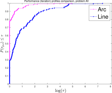
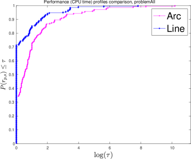
Figure 1: Performance profiles of the number of iterations (left) and the computation time (right) for all solvable problems.

Figures 2 illustrates the performance profile for QCQPs. This result indicates that the computation time of the proposed arc-search algorithm is competitive with the line-search algorithm in QCQPs. The degrees of the functions in QCQPs are at most 2, therefore, the approximation with the ellipse fits the central path well and the number of iterations is much smaller than the line-search algorithm.

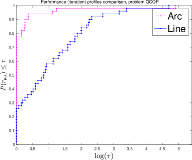
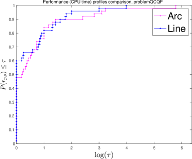
Figure 2: Performance profiles of the number of iterations (left) and the computation time (right) for QCQP problems

5.2 High-order derivatives

As pointed out above, the main bottleneck of the proposed arc-search algorithm is the computation of the high-order derivatives; $(\nabla_{x}^{3}L(v))\dot{x}\dot{x}$, $(\nabla_{x}^{2}h(x))\dot{y}\dot{x}$, $(\nabla_{g}^{2}h(x))\dot{z}\dot{x}$, $(\nabla_{x}^{2}h(x))\dot{x}\dot{x}$, and $(\nabla_{x}^{2}g(x))\dot{z}\dot{x})$. However, these higher-order derivatives appear only in the right-hand side of (37) for obtaining $\ddot{v}$. Since the second-order approximation $\ddot{v}$ gives a less influence on ${v}(\alpha)$ than the first-order approximation $\dot{v}$ when $\alpha$ is small, we can expect that small deviations in the computation of $\ddot{v}$ would not affect the approximation of ${v}$ so much. In addition, we can remove the effect of numerical errors in the numerical differentiations like (63). Based on these intuitions, we examine another approximation with $\ddot{\ddot{v}}=(\ddot{\ddot{x}},\ddot{\ddot{y}},\ddot{\ddot{w}},\ddot{\ddot{s}},\ddot{\ddot{z}})$ defined as the solution of the following system in which we ignored the higher-order derivatives of (37):

$$\left[\begin{array}[]{ccccc}\nabla_{x}^{2}L(v)&\nabla h(x)&-\nabla g(x)&0&0\\ \left(\nabla h(x)\right)^{{\rm T}}&0&0&0&0\\ \left(\nabla g(x)\right)^{{\rm T}}&0&0&-I&0\\ 0&0&I&0&-I\\ 0&0&0&{\cal D}({z})&{\cal D}({s})\end{array}\right]\left[\begin{array}[]{c}\ddot{\ddot{x}}\\ \ddot{\ddot{y}}\\ \ddot{\ddot{w}}\\ \ddot{\ddot{s}}\\ \ddot{\ddot{z}}\end{array}\right] = \left[\begin{array}[]{l}0\\ 0\\ 0\\ 0\\ -2{\cal D}(\dot{z})\dot{s}\end{array}\right].$$ (79)

Figure 3 compares the arc-search algorithm with $\ddot{\ddot{v}}$ and the line-search algorithm (Algorithm 5.1) using the performance profiling. In the viewpoint of the number of iterations, the arc-search algorithm keeps its superiority. In addition, the arc-search algorithm solves the problems in a shorter time than the line-search algorithm, since we skip the main bottlenecks.

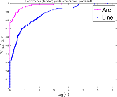
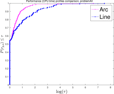
Figure 3: Performance profiles of the number of iterations (left) and the computation time (right) with the use of $\ddot{\ddot{v}}$

Since $\ddot{\ddot{v}}$ can not draw the ellipse ${\cal E}$ exactly, we cannot apply the same theoretical developments in the previous section. However, these numerical results give promising insights for further improvements on the arc-search algorithm.

6 Conclusions

In this paper, we extend the arc-search algorithm, which approximates the central path with an arc of the ellipse, for NLPs and also discuss the convergence of the proposed algorithm. From the results of numerical experiments, the arc-search algorithm succeeded in reducing the number of iterations compared with the line-search algorithm.

As a future work, we should focus the computation time reduction of the arc-search algorithm. In particular, we expect the drop of the high-order derivatives in the computation of $\ddot{v}$ will bring us an enhancement of the algorithm as observed in Section 5.2, though the deviation from the arc due to the drop should be theoretically addressed. We should also incorporate some implementation techniques to improve the numerical stability for NLPs.

Appendix Appendix A Derivatives

In this section, we give notation related to derivatives. The Hessian matrix of $f:{\mathbb{R}}^{n}\to{\mathbb{R}}$ is

$$\nabla^{2}f(x)=\left[\begin{array}[]{cccc}\frac{\partial^{2}f}{\partial x_{1}\partial x_{1}}&\frac{\partial^{2}f}{\partial x_{1}\partial x_{2}}&\cdots&\frac{\partial^{2}f}{\partial x_{1}\partial x_{n}}\\ \vdots&\vdots&\ddots&\vdots\\ \frac{\partial^{2}f}{\partial x_{n}\partial x_{1}}&\frac{\partial^{2}f}{\partial x_{n}\partial x_{2}}&\cdots&\frac{\partial^{2}f}{\partial x_{n}\partial x_{n}}\end{array}\right]\in{\mathbb{R}}^{n\times n}.$$

The Jacobian for $h:{\mathbb{R}}^{n}\to{\mathbb{R}}^{m}$ is

$$\nabla h(x)=\left[\begin{array}[]{cccc}\frac{\partial h_{1}}{\partial x_{1}}&\frac{\partial h_{2}}{\partial x_{1}}&\cdots&\frac{\partial h_{m}}{\partial x_{1}}\\ \vdots&\vdots&\ddots&\vdots\\ \frac{\partial h_{1}}{\partial x_{n}}&\frac{\partial h_{2}}{\partial x_{n}}&\cdots&\frac{\partial h_{m}}{\partial x_{n}}\end{array}\right]=[\nabla h_{1}(x),\cdots,\nabla h_{m}(x)]\in{\mathbb{R}}^{n\times m}.$$

The Jacobian for $g:{\mathbb{R}}^{n}\to{\mathbb{R}}^{p}$ is

$$\nabla g(x)=\left[\begin{array}[]{cccc}\frac{\partial g_{1}}{\partial x_{1}}&\frac{\partial g_{2}}{\partial x_{1}}&\cdots&\frac{\partial g_{p}}{\partial x_{1}}\\ \vdots&\vdots&\ddots&\vdots\\ \frac{\partial g_{1}}{\partial x_{n}}&\frac{\partial g_{2}}{\partial x_{n}}&\cdots&\frac{\partial g_{p}}{\partial x_{n}}\end{array}\right]=[\nabla g_{1}(x),\cdots,\nabla g_{p}(x)]\in{\mathbb{R}}^{n\times p}.$$

For the right-hand-side of (37), we use

$$\nabla_{x}^{3}L(x,y,z)\dot{x}\dot{x} = \frac{\partial\left(\frac{\partial^{2}L(x,y,z)}{\partial x^{2}}\dot{x}\right)}{\partial x}\dot{x}=\sum_{i=1}^{n}\dot{x}_{i}\frac{\partial}{\partial x}\left[\begin{array}[]{c}\frac{\partial^{2}L(x,y,z)}{\partial x_{1}\partial x_{i}}\\ \vdots\\ \frac{\partial^{2}L(x,y,z)}{\partial x_{n}\partial x_{i}}\end{array}\right]\dot{x}$$

$$\nabla_{x}^{2}h(x)\dot{y}\dot{x} = \frac{\partial\left(\frac{\partial h(x)}{\partial x}\dot{y}\right)}{\partial x}\dot{x}=\sum_{i=1}^{m}\dot{y}_{i}\frac{\partial}{\partial x}\left[\begin{array}[]{c}\frac{\partial h_{i}(x)}{\partial x_{1}}\\ \vdots\\ \frac{\partial h_{i}(x)}{\partial x_{n}}\end{array}\right]\dot{x}=\sum_{i=1}^{m}\dot{y}_{i}\left(\nabla_{x}^{2}h_{i}(x)\right)\dot{x}$$

$$\nabla_{x}^{2}g(x)\dot{z}\dot{x} = \frac{\partial\left(\frac{\partial g(x)}{\partial x}\dot{z}\right)}{\partial x}\dot{x}=\sum_{i=1}^{n}\dot{z}_{i}\frac{\partial}{\partial x}\left[\begin{array}[]{c}\frac{\partial g_{i}(x)}{\partial x_{1}}\\ \vdots\\ \frac{\partial g_{i}(x)}{\partial x_{n}}\end{array}\right]\dot{x}=\sum_{i=1}^{n}\dot{z}_{i}\left(\nabla_{x}^{2}g_{i}(x)\right)\dot{x}$$

$$\nabla_{x}^{2}h(x)^{{\rm T}}\dot{x}\dot{x} = \left(\frac{\partial\left(\left(\frac{\partial h(x)}{\partial x}\right)^{{\rm T}}\dot{x}\right)}{\partial x}\right)^{{\rm T}}\dot{x}=\left[\begin{array}[]{c}\dot{x}^{{\rm T}}\left(\nabla_{x}^{2}h_{1}(x)\right)\dot{x}\\ \vdots\\ \dot{x}^{{\rm T}}\left(\nabla_{x}^{2}h_{m}(x)\right)\dot{x}\end{array}\right]$$

$$\nabla_{x}^{2}g(x)^{{\rm T}}\dot{x}\dot{x} = \left(\frac{\partial\left(\left(\frac{\partial g(x)}{\partial x}\right)^{{\rm T}}\dot{x}\right)}{\partial x}\right)^{{\rm T}}\dot{x}=\left[\begin{array}[]{c}\dot{x}^{{\rm T}}\left(\nabla_{x}^{2}g_{1}(x)\right)\dot{x}\\ \vdots\\ \dot{x}^{{\rm T}}\left(\nabla_{x}^{2}g_{p}(x)\right)\dot{x}\end{array}\right].$$

Appendix Appendix B The largest step angle

In this section, we give analytical forms to compute the largest $\alpha_{w_{i}}$ and $\alpha_{s_{i}}$ for each $i$ in (41). For simplicity, here, we drop the index $i$ and the iteration number $k$; for example, $w_{i}^{k}$ is simply written as $w$. For (40a), we should have

$$w(\alpha)=w-\dot{w}\sin(\alpha)+\ddot{w}(1-\cos(\alpha))\geq\delta w,$$

or equivalently,

$$w-\delta w+\ddot{w}\geq\dot{w}\sin(\alpha)+\ddot{w}\cos(\alpha).$$ (84)

We split this computation into seven cases by the signs of $\dot{w}$ and $\ddot{w}$.

Case 1 ($\dot{w}=0$ and $\ddot{w}\neq 0$):

If $\ddot{w}\geq-(1-\delta)w$, then $w(\alpha)\geq\delta w$ holds for $\alpha\in[0,\frac{\pi}{2}]$. If $\ddot{w}\leq-(1-\delta)w<0$, to meet (84), we must have $\cos(\alpha)\geq\frac{w-\delta w+\ddot{w}}{\ddot{w}}\geq 0$, or, $\alpha\leq\cos^{-1}\left(\frac{w-\delta w+\ddot{w}}{\ddot{w}}\right)$. Therefore,

$$\alpha_{w}=\left\{\begin{array}[]{ll}\frac{\pi}{2}&\quad\mbox{if $w-\delta w+\ddot{w}\geq 0$}\\ \cos^{-1}\left(\frac{w-\delta w+\ddot{w}}{\ddot{w}}\right)&\quad\mbox{if $w-\delta w+\ddot{w}\leq 0$}.\end{array}\right.$$

Case 2 ($\ddot{w}=0$ and $\dot{w}\neq 0$):

If $\dot{w}\leq(1-\delta)w$, then $w(\alpha)\geq\delta w$ holds for any $\alpha\in[0,\frac{\pi}{2}]$. If $\dot{w}\geq(1-\delta)w>0$, to meet (84), we must have $\sin(\alpha)\leq\frac{w-\delta w}{\dot{w}}$, or $\alpha\leq\sin^{-1}\left(\frac{w-\delta w}{\dot{w}}\right)$. Therefore,

$$\alpha_{w}=\left\{\begin{array}[]{ll}\frac{\pi}{2}&\quad\mbox{if $\dot{w}\leq w-\delta w$}\\ \sin^{-1}\left(\frac{w-\delta w}{\dot{w}}\right)&\quad\mbox{if $\dot{w}\geq w-\delta w$}.\end{array}\right.$$

Case 3 ($\dot{w}>0$ and $\ddot{w}>0$):

Let $\beta=\sin^{-1}\left(\frac{\ddot{w}}{\sqrt{\dot{w}^{2}+\ddot{w}^{2}}}\right)$. We can express $\dot{w}=\sqrt{\dot{w}^{2}+\ddot{w}^{2}}\cos(\beta)$ and $\ddot{w}=\sqrt{\dot{w}^{2}+\ddot{w}^{2}}\sin(\beta)$. Then, (84) can be rewritten as

$$w-\delta w+\ddot{w}\geq\sqrt{\dot{w}^{2}+\ddot{w}^{2}}\sin(\alpha+\beta).$$ (85)

If $\ddot{w}+w-\delta w\geq\sqrt{\dot{w}^{2}+\ddot{w}^{2}}$, then $w(\alpha)\geq\delta w$ holds for any $\alpha\in[0,\frac{\pi}{2}]$. If $\ddot{w}+w-\delta w\leq\sqrt{\dot{w}^{2}+\ddot{w}^{2}}$, to meet (85), we must have $\sin(\alpha+\beta)\leq\frac{w-\delta w+\ddot{w}}{\sqrt{\dot{w}^{2}+\ddot{w}^{2}}}$, or $\alpha+\beta\leq\sin^{-1}\left(\frac{w-\delta w+\ddot{w}}{\sqrt{\dot{w}^{2}+\ddot{w}^{2}}}\right)$. Therefore,

$$\alpha_{w}=\left\{\begin{array}[]{ll}\frac{\pi}{2}&\quad\mbox{if $w-\delta w+\ddot{w}\geq\sqrt{\dot{w}^{2}+\ddot{w}^{2}}$}\\ \sin^{-1}\left(\frac{w-\delta w+\ddot{w}}{\sqrt{\dot{w}^{2}+\ddot{w}^{2}}}\right)-\sin^{-1}\left(\frac{\ddot{w}}{\sqrt{\dot{w}^{2}+\ddot{w}^{2}}}\right)&\quad\mbox{if $w-\delta w+\ddot{w}\leq\sqrt{\dot{w}^{2}+\ddot{w}^{2}}$}.\end{array}\right.$$

Case 4 ($\dot{w}>0$ and $\ddot{w}<0$):

Let $\beta=\sin^{-1}\left(\frac{-\ddot{w}}{\sqrt{\dot{w}^{2}+\ddot{w}^{2}}}\right)$. We can express $\dot{w}=\sqrt{\dot{w}^{2}+\ddot{w}^{2}}\cos(\beta)$ and $\ddot{w}=-\sqrt{\dot{w}^{2}+\ddot{w}^{2}}\sin(\beta)$. Then, (84) can be rewritten as

$$w-\delta w+\ddot{w}\geq\sqrt{\dot{w}^{2}+\ddot{w}^{2}}\sin(\alpha-\beta).$$ (86)

If $\ddot{w}+w-\delta w\geq\sqrt{\dot{w}^{2}+\ddot{w}^{2}}$, then $w(\alpha)\geq\delta w$ holds for any $\alpha\in[0,\frac{\pi}{2}]$. If $\ddot{w}+w-\delta w\leq\sqrt{\dot{w}^{2}+\ddot{w}^{2}}$, to meet (86), we must have $\sin(\alpha-\beta)\leq\frac{w-\delta w+\ddot{w}}{\sqrt{\dot{w}^{2}+\ddot{w}^{2}}}$, or $\alpha-\beta\leq\sin^{-1}\left(\frac{w-\delta w+\ddot{w}}{\sqrt{\dot{w}^{2}+\ddot{w}^{2}}}\right)$. Therefore,

$$\alpha_{w}=\left\{\begin{array}[]{ll}\frac{\pi}{2}&\quad\mbox{if $w-\delta w+\ddot{w}\geq\sqrt{\dot{w}^{2}+\ddot{w}^{2}}$}\\ \sin^{-1}\left(\frac{w-\delta w+\ddot{w}}{\sqrt{\dot{w}^{2}+\ddot{w}^{2}}}\right)+\sin^{-1}\left(\frac{-\ddot{w}}{\sqrt{\dot{w}^{2}+\ddot{w}^{2}}}\right)&\quad\mbox{if $w-\delta w+\ddot{w}\leq\sqrt{\dot{w}^{2}+\ddot{w}^{2}}$}.\end{array}\right.$$

Case 5 ($\dot{w}<0$ and $\ddot{w}<0$):

Let $\beta=\sin^{-1}\left(\frac{-\ddot{w}}{\sqrt{\dot{w}^{2}+\ddot{w}^{2}}}\right)$. We can express $\dot{w}=-\sqrt{\dot{w}^{2}+\ddot{w}^{2}}\cos(\beta)$ and $\ddot{w}=-\sqrt{\dot{w}^{2}+\ddot{w}^{2}}\sin(\beta)$. Then, (84) can be rewritten as

$$w-\delta w+\ddot{w}\geq-\sqrt{\dot{w}^{2}+\ddot{w}^{2}}\sin(\alpha+\beta),$$ (87)

If $\ddot{w}+(w-\delta w)\geq 0$, then $w(\alpha)\geq\delta w$ holds for any $\alpha\in[0,\frac{\pi}{2}]$. If $\ddot{w}+(w-\delta w)\leq 0$, to meet (87), we must have $\sin(\alpha+\beta)\geq\frac{-(w-\delta w+\ddot{w})}{\sqrt{\dot{w}^{2}+\ddot{w}^{2}}}$, or $\alpha+\beta\leq\pi-\sin^{-1}\left(\frac{-(w-\delta w+\ddot{w})}{\sqrt{\dot{w}^{2}+\ddot{w}^{2}}}\right)$. Therefore,

$$\alpha_{w}=\left\{\begin{array}[]{ll}\frac{\pi}{2}&\quad\mbox{if $w-\delta w+\ddot{w}\geq 0$}\\ \pi-\sin^{-1}\left(\frac{-(w-\delta w+\ddot{w})}{\sqrt{\dot{w}^{2}+\ddot{w}^{2}}}\right)-\sin^{-1}\left(\frac{-\ddot{w}}{\sqrt{\dot{w}^{2}+\ddot{w}^{2}}}\right)&\quad\mbox{if $w-\delta w+\ddot{w}\leq 0$}.\end{array}\right.$$

Case 6 ($\dot{w}<0$ and $\ddot{w}>0$):

Clearly (84) always holds for any $\alpha\in[0,\frac{\pi}{2}]$. Therefore, we can take

$$\alpha_{w}=\frac{\pi}{2}.$$ (88)

Case 7 ($\dot{w}=0$ and $\ddot{w}=0$):

Clearly (84) always holds for any $\alpha\in[0,\frac{\pi}{2}]$. Therefore, we can take

$$\alpha_{w}=\frac{\pi}{2}.$$ (89)

Similar analysis can be performed for (40b), then similar analytical forms are derived for $\alpha_{s}$.

Appendix Appendix C Details on Numerical Results

Tables 1, 2 and 3 report the objective value, the numbers of iterations, and the computation time (in seconds) of the proposed arc-search algorithm (Algorithm 3.1) and the line-search algorithm (Algorithm 5.1) for QCQP and Other type problems. The symbol “Unattained” indicates that the algorithms stopped prematurely, mainly because of the numerical errors. We excluded the problems that all the three algorithms (Algorithm 3.1, Algorithm 3.1 with $\ddot{\ddot{v}}$, and Algorithm 5.1) stopped with “Unattained”.

Table 1: Results on QCQP problems

	arc-search (Algorithm 3.1)			line-search (Algorithm 5.1)			arc-search with $\ddot{\ddot{v}}$ in (79)
Problem	Obj	Iter	Time	Obj	Iter	Time	Obj	Iter	Time
BT12	6.1881	4	0.014	6.1881	20	0.009	6.1881	3	0.005
TRY-B	0.0000	12	0.009	1.0000	10	0.004	0.0000	18	0.011
BT1	-1.0001	11	0.017	-0.9937	21	0.013	-0.9991	8	0.011
BT2	0.0326	10	0.006	0.0326	22	0.009	0.0326	11	0.006
BT4	4.6075	8	0.007	4.6075	20	0.008	4.6075	5	0.003
BT5	967.6665	6	0.005	961.7151	22	0.009	961.7152	5	0.003
BT8	1.0000	4	0.009	1.0000	19	0.022	1.0001	7	0.012
HS108	-0.8661	9	0.011	-0.5000	22	0.013	Unattained
HS113	24.3061	13	0.012	24.3058	11	0.006	24.3059	9	0.005
HS12	-30.0000	8	0.022	-30.0001	15	0.017	-30.0000	12	0.020
HS22	0.9999	6	0.005	0.9999	5	0.002	1.0000	5	0.003
HS30	0.9999	10	0.008	0.9999	9	0.004	0.9999	10	0.006
HS31	5.9994	10	0.008	5.9993	9	0.004	5.9994	11	0.007
HS43	-44.0003	8	0.007	-44.0002	11	0.006	-44.0003	9	0.006
HS63	961.7152	9	0.008	961.7151	7	0.003	961.7152	10	0.006
HS65	0.9535	12	0.010	0.9535	10	0.006	0.9535	15	0.010
HS83	-30670.0988	20	0.018	-30670.0999	21	0.010	-30670.0991	21	0.013
MARATOS	-1.0000	3	0.002	-1.0000	14	0.006	-1.0000	3	0.002
OPTPRLOC	Unattained			Unattained			-16.4211	44	0.077
ORTHREGB	0.0000	1	0.002	0.0000	26	0.016	0.0000	1	0.001
ZECEVIC3	97.3087	9	0.006	97.3086	10	0.005	97.3087	9	0.005
ZECEVIC4	7.5574	9	0.006	7.5575	7	0.003	7.5575	8	0.004
HS11	-8.4988	7	0.005	-8.4985	13	0.006	-8.4987	8	0.004
HS14	1.3933	5	0.015	1.3934	9	0.011	1.3934	6	0.011
HS18	5.0000	11	0.008	5.0000	14	0.007	5.0000	14	0.008
HS27	Unattained			0.0400	24	0.012	0.0400	27	0.023
HS42	13.8579	3	0.002	13.8579	19	0.008	13.8579	3	0.002
HS57	0.0306	9	0.007	0.0285	16	0.012	0.0305	15	0.009
BT13	-0.0001	10	0.026	-0.0001	17	0.026	Unattained
CONGIGMZ	Unattained			Unattained			27.9991	20	0.011
GIGOMEZ1	-2.9999	40	0.036	-3.0000	421	0.569	-3.0001	72	0.093
HAIFAM	-45.0004	287	14.955	-45.0004	1000	9.007	-45.0003	1000	14.112
HAIFAS	-0.4499	5	0.015	-0.4501	20	0.026	-0.4499	6	0.011
HS10	-1.0000	7	0.005	-1.0001	8	0.004	-1.0000	9	0.005
MAKELA1	-1.4143	34	0.032	-1.4143	107	0.109	-1.4143	17	0.014
MAKELA2	7.1999	7	0.005	7.2000	7	0.003	7.2000	7	0.004
MAKELA3	0.0006	12	0.019	0.0000	19	0.013	Unattained
MIFFLIN1	-0.9999	5	0.003	-1.0001	6	0.003	-1.0000	5	0.003
MIFFLIN2	-1.0000	7	0.005	-1.0001	10	0.005	-1.0001	13	0.008
MINMAXRB	-0.0001	332	0.331	-0.0001	11	0.006	0.0000	10	0.007
POLAK4	Unattained			Unattained			-0.0001	365	0.388
PRODPL0	58.7752	33	0.225	58.7769	14	0.024	58.7759	21	0.058
PRODPL1	35.7313	28	0.188	35.7281	13	0.022	35.7298	17	0.048
ROSENMMX	-44.0000	10	0.007	-44.0001	15	0.007	-43.9999	10	0.005
SMMPSF	1032924.7420	31	192.294	1032924.7330	68	36.244	1032924.7420	30	29.892
SWOPF	0.0679	26	0.333	0.0679	26	0.047	0.0679	19	0.051
TRUSPYR1	11.2255	8	0.020	11.2254	12	0.014	11.2256	8	0.014
TRUSPYR2	11.2203	9	0.009	11.2200	24	0.017	11.2204	12	0.009
COOLHANS	0.0000	5	0.006	0.0000	20	0.011	0.0000	8	0.005
GOTTFR	0.0000	6	0.005	0.0000	18	0.010	0.0000	5	0.003
HIMMELBC	0.0000	7	0.005	0.0000	21	0.009	0.0000	4	0.002
HIMMELBE	0.0000	2	0.002	0.0000	18	0.007	0.0000	2	0.001
HYPCIR	0.0000	4	0.003	0.0000	18	0.008	0.0000	4	0.002
HS8	-1.0000	6	0.004	-1.0000	21	0.010	-1.0000	4	0.002

Table 2: Results on Others

	arc-search (Algorithm 3.1)			line-search (Algorithm 5.1)			arc-search with $\ddot{\ddot{v}}$ in (79)
Problem	Obj	Iter	Time	Obj	Iter	Time	Obj	Iter	Time
ACOPR30	576.8530	22	1.035	576.8530	122	0.805	576.8513	37	0.438
ACOPR30	Unattained			Unattained			576.8530	956	11.482
ACOPR57	41737.7220	271	53.130	41737.7230	107	2.513	41737.7231	30	1.091
ARGAUSS	0.0000	1	0.009	0.0000	1	0.007	0.0000	1	0.008
BA-L1	0.0000	4	0.036	0.0000	23	0.040	0.0000	3	0.008
BA-L1SP	0.0000	9	0.139	0.0000	24	0.063	0.0000	6	0.022
BT6	0.2770	7	0.006	0.2770	18	0.008	0.2770	10	0.006
BT7	306.5000	26	0.026	403.9997	30	0.015	360.3798	12	0.008
BT9	-1.0000	16	0.015	-1.0000	28	0.013	-1.0000	12	0.007
BT10	-1.0000	4	0.003	-1.0000	18	0.007	-1.0000	6	0.003
BT11	0.8249	6	0.005	0.8249	21	0.009	0.8249	7	0.004
CANTILVR	Unattained			Unattained			1.3399	11	0.007
CB2	1.9523	6	0.004	1.9521	8	0.004	1.9522	7	0.004
CB3	2.0000	8	0.006	1.9999	9	0.005	2.0000	7	0.004
CHACONN1	1.9522	9	0.006	1.9521	7	0.003	1.9522	6	0.003
CHACONN2	1.9999	7	0.005	1.9999	8	0.004	2.0000	7	0.004
CLUSTER	Unattained			Unattained			0.0000	5	0.007
CUBENE	0.0000	4	0.003	0.0000	47	0.032	0.0000	4	0.003
DIPIGRI	680.6300	16	0.013	680.6299	15	0.007	680.6300	15	0.009
DIXCHLNG	2471.8978	9	0.009	2471.8978	33	0.016	2471.8978	9	0.005
FLETCHER	Unattained			Unattained			19.5232	14	0.017
HALDMADS	Unattained			Unattained			0.0346	48	0.059
HATFLDF	0.0000	6	0.005	0.0000	15	0.007	Unattained
HATFLDG	0.0000	18	0.052	0.0000	21	0.014	0.0000	5	0.006
HEART8	0.0000	117	0.584	0.0000	469	1.838	0.0000	447	2.072
HELIXNE	0.0000	5	0.004	0.0000	25	0.011	0.0000	8	0.004
HIMMELBI	-1735.5689	20	0.496	-1735.5698	18	0.090	-1735.5689	20	0.180
HIMMELBK	0.0517	17	0.042	0.0516	37	0.038	0.0516	58	0.087
HIMMELP4	-8.1980	42	0.029	-8.1980	20	0.010	Unattained
HONG	22.5711	11	0.010	22.5711	10	0.006	22.5711	8	0.006
HS100	680.6300	16	0.013	680.6299	15	0.007	680.6300	15	0.008
HS100LNP	Unattained			Unattained			680.6301	7	0.014
HS100MOD	678.6796	22	0.018	678.6795	14	0.007	678.6795	20	0.011
HS101	1808.9319	174	0.254	1808.9335	463	0.486	Unattained
HS104	3.9502	10	0.010	3.9501	11	0.006	3.9502	10	0.007
HS111	Unattained			-45.8493	15	0.009	-47.7612	16	0.014
HS111LNP	-43.1482	17	0.030	-45.8490	19	0.009	-45.8494	10	0.006
HS112	-47.7611	25	0.027	-47.7611	19	0.011	-47.7611	28	0.022
HS114	Unattained			-1770.6936	27	0.016	-1770.6934	30	0.024
HS119	244.8788	14	0.018	244.8790	12	0.010	244.8788	15	0.013
HS24	-1.0000	9	0.007	0.0000	11	0.007	-1.0001	8	0.004
HS26	0.0000	12	0.008	0.0000	21	0.009	0.0000	12	0.006
HS29	-22.6275	7	0.005	0.0000	19	0.015	-22.6274	6	0.004
HS32	0.9997	5	0.015	0.9996	6	0.009	0.9997	5	0.010
HS34	Unattained			-0.8341	45	0.021	-0.8341	59	0.032
HS36	-3300.2088	12	0.009	-0.0001	10	0.005	-3300.2088	12	0.008
HS37	0.0000	15	0.010	-0.0001	11	0.005	0.0000	1000	0.492
HS39	-1.0000	16	0.015	-1.0000	28	0.013	-1.0000	12	0.007
HS40	-0.2500	3	0.002	-0.2500	15	0.006	-0.2500	3	0.002
HS41	1.9259	8	0.006	1.9259	6	0.003	1.9259	7	0.004
HS46	Unattained			Unattained			0.0000	12	0.006
HS49	0.0000	12	0.008	0.0000	26	0.011	0.0000	13	0.007
HS50	0.0000	4	0.003	0.0000	31	0.013	0.0000	8	0.004

Table 3: Results on Others (continued)

	arc-search (Algorithm 3.1)			line-search (Algorithm 5.1)			arc-search with $\ddot{\ddot{v}}$ in (79)
Problem	Obj	Iter	Time	Obj	Iter	Time	Obj	Iter	Time
HS55	6.3333	6	0.013	6.3332	6	0.008	6.3333	6	0.010
HS56	0.0000	14	0.013	0.0000	20	0.009	0.0000	14	0.008
HS59	-7.8027	42	0.031	-7.8028	18	0.010	-6.7495	204	0.151
HS60	0.0326	11	0.009	0.0326	11	0.006	0.0326	11	0.007
HS64	Unattained			Unattained			6299.6148	19	0.012
HS66	Unattained			Unattained			0.5182	60	0.032
HS68	0.0000	21	0.018	0.0000	10	0.005	0.0000	21	0.015
HS69	0.0040	49	0.046	0.0040	183	0.166	0.0040	52	0.042
HS7	1.7844	9	0.007	1.7844	27	0.016	1.7321	16	0.014
HS71	Unattained			Unattained			17.0139	16	0.018
HS73	29.8944	5	0.015	29.8943	7	0.009	29.8944	5	0.010
HS74	5126.4981	18	0.019	5126.4981	18	0.009	5126.4981	17	0.014
HS75	5174.1355	23	0.022	5174.1352	15	0.007	5174.1355	23	0.017
HS77	0.2415	8	0.006	0.2415	18	0.008	0.2415	8	0.004
HS78	-2.9197	3	0.002	-2.9197	20	0.008	-2.9197	3	0.002
HS79	0.0788	3	0.003	0.0788	19	0.008	0.0788	4	0.002
HS86	Unattained			Unattained			-32.3506	17	0.010
HS99	-831079891.5000	8	0.007	-831079891.5000	35	0.017	-831079891.5000	8	0.005
HUBFIT	0.0169	5	0.003	0.0169	5	0.003	0.0169	5	0.003
HYDCAR20	0.0000	16	0.495	0.0000	20	0.066	0.0000	8	0.042
HYDCAR6	0.0000	6	0.019	0.0000	22	0.017	0.0000	4	0.005
LAKES	350525.0229	35	0.481	350524.9285	60	0.100	350525.0229	43	0.136
LEAKNET	8.0448	55	3.482	8.0020	38	0.187	8.0449	41	0.362
LIN	-0.0176	5	0.004	-0.0176	13	0.006	-0.0176	5	0.003
LOADBAL	0.4529	34	0.075	0.4531	26	0.025	0.4529	34	0.046
LOOTSMA	8.0000	10	0.009	7.7990	1000	0.442	8.0000	18	0.010
LSNNODOC	123.1027	18	0.029	123.1026	11	0.013	123.1027	23	0.030
MADSEN	0.6164	8	0.006	0.6163	11	0.005	Unattained
MATRIX2	0.0001	7	0.006	0.0001	11	0.007	0.0000	28	0.024
METHANB8	0.0000	2	0.007	0.0000	17	0.013	0.0000	2	0.003
METHANL8	0.0000	3	0.010	0.0000	23	0.018	0.0000	3	0.004
MINMAXBD	115.7064	33	0.041	115.7064	50	0.028	115.7064	36	0.024
MWRIGHT	42.0461	8	0.007	42.0461	24	0.010	42.0461	5	0.003
ODFITS	-2380.0268	48	0.038	-2380.0268	20	0.010	-2380.0268	14	0.008
POLAK1	2.7183	9	0.006	2.7182	13	0.006	2.7182	8	0.004
POLAK2	54.5982	7	0.006	54.5981	10	0.005	54.5982	7	0.004
POLAK3	5.9329	138	0.178	5.9329	12	0.006	5.9329	11	0.007
POLAK5	49.9999	46	0.038	49.9999	10	0.004	50.0000	7	0.004
POLAK6	Unattained			Unattained			-44.0000	22	0.013
POWELLBS	0.0000	6	0.004	0.0000	17	0.008	0.0000	40	0.031
RECIPE	0.0000	5	0.004	0.0000	19	0.008	0.0000	9	0.005
RES	0.0000	29	0.042	0.0000	18	0.011	0.0000	29	0.028
SINVALNE	0.0000	7	0.005	0.0000	28	0.016	0.0000	3	0.002
SMBANK	-7129292.0000	55	2.151	-7129292.0000	196	1.709	-7129292.0000	64	0.834
SYNTHES1	0.7573	7	0.006	0.7573	7	0.004	0.7573	7	0.004
SYNTHES2	-0.5639	9	0.012	-0.5636	9	0.006	-0.5638	9	0.008
SYNTHES3	15.0732	13	0.020	15.0733	10	0.007	15.0730	10	0.010
TRIGGER	0.0000	6	0.020	0.0000	1000	4.509	0.0000	10	0.026
TRIMLOSS	Unattained			9.0559	142	1.778	9.0599	253	5.672
TWOBARS	1.5086	6	0.004	1.5084	6	0.003	1.5086	6	0.003
WATER	10549.3616	31	0.131	10549.3602	34	0.064	10549.3616	28	0.073
ZY2	7.8905	7	0.007	7.8904	7	0.005	7.8904	8	0.006
ACOPR118	129660.2236	203	323.214	129660.2294	54	10.248	129660.2319	32	10.623
ALSOTAME	0.0821	8	0.005	0.0821	7	0.004	0.0821	7	0.004

References

- [1] R. H. Byrd, J. C. Gilbert, and J. Nocedal, A trust region method based on interior point techniques for nonlinear programming, Mathematical Programming, 89 (2000), pp. 149–185.
- [2] R. H. Byrd, M. E. Hribar, and J. Nocedal, An interior point algorithm for large-scale nonlinear programming, SIAM Journal on Optimization, 9 (1999), pp. 877–900.
- [3] A. S. El-Bakry, R. A. Tapia, T. Tsuchiya, and Y. Zhang, On the formulation and theory of the Newton interior-point method for nonlinear programming, Journal of Optimization Theory and Applications, 89 (1996), pp. 507–541.
- [4] A. Forsgren and P. E. Gill, Primal-dual interior methods for nonconvex nonlinear programming, SIAM Journal on Optimization, 8 (1998), pp. 1132–1152.
- [5] N. Gould and J. Scott, A note on performance profiles for benchmarking software, ACM Transactions on Mathematical Software, 43 (2016), p. 15.
- [6] N. I. Gould, D. Orban, and P. L. Toint, CUTEst: a constrained and unconstrained testing environment with safe threads for mathematical optimization, Computational Optimization and Applications, 60 (2015), pp. 545–557.
- [7] B. Kheirfam, An arc-search infeasible interior-point algorithm for horizontal linear complementarity problem in the neighbourhood of the central path, International Journal of Computer Mathematics, 94 (2017), pp. 2271–2282.
- [8] T. Lu and S. Shiou, Inverses of 2 2 block matrices, Computers and Mathematics with Applications, 43 (2002), pp. 119–129.
- [9] I. Lustig, R. Marsten, and D. Shannon, Computational experience with a primal-dual interior-point method for linear programming, Linear Algebra and Its Applications, 152 (1991), pp. 192–222.
- [10] , On implementing Mehrotra’s predictor-corrector interior-point method for linear programming, SIAM Journal on Optimization, 2 (1992), pp. 432–449.
- [11] S. Mehrotra, On the implementation of a primal-dual interior point method, SIAM Journal on Optimization, 2 (1992), pp. 575–601.
- [12] J. Nocedal, A. Wachter, and R. A. Waltz, Adaptive barrier update strategies for nonlinear interior methods, SIAM Journal on Optimization, 19 (2009), pp. 1674–1693.
- [13] T. Plantenga, A trust region method for nonlinear programming based on primal interior-point techniques, SIAM Journal on Optimization, 20 (1998), p. 282â305.
- [14] A. L. Tits, A. Wachter, S. Bakhtiarl, T. J. Urban, and C. T. Lawrence, A primal-dual method for nonlinear programming with strong global and local convergence properties, Mathematical Programming, 8 (1998), pp. 1132–1152.
- [15] M. Ulbrich, S. Ulbrich, and L. N. Vicente, A globally convergent primal-dual interior-point filter method for nonlinear programming, Mathematical Programming, 100 (2004), pp. 379–410.
- [16] R. Vanderbei and D. Shanno, An interior-point algorithm for nonconvex nonlinear programming, Computational Optimization and Applications, 13 (1999), pp. 231–252.
- [17] S. Wright, Primal-Dual Interior-Point Methods, SIAM, Philadelphia, 1997.
- [18] X. Yang, H. Liu, and Y. Zhang, An arc-search infeasible-interior-point method for symmetric optimization in a wide neighborhood of the central path, Optimization Letters, 11 (2017), pp. 135–152.
- [19] Y. Yang, A polynomial arc-search interior-point algorithm for convex quadratic programming, European Journal of Operational Research, 215 (2011), p. 25â38.
- [20] Y. Yang, A polynomial arc-search interior-point algorithm for linear programming, Journal of Optimization Theory and Applications, 158 (2013), pp. 859–873.
- [21] , Curvelp-a matlab implementation of an infeasible interior-point algorithm for linear programming, Numerical Algorithms, 74 (2017), p. 967â996.
- [22] , Two computationally efficient polynomial-iteration infeasible interior-point algorithms for linear programming, Numerical Algorithms, 79 (2018), p. 957â992.
- [23] Y. Yang and M. Yamashita, An arc-search infeasible-interior-point algorithm for linear programming, Optimization Letters, 12 (2018), pp. 781–798.
- [24] Y. Ye, Interior Point Algorithms: Theory and Analysis, John Wiley & Son, Inc, New York, 1997.
- [25] M. Zhang, B. Yuan, Y. Zhou, X. Luo, and Z. Huang, A primal-dual interior-point algorithm with arc-search for semidefinite programming, Optimization Letters, 13 (2019), pp. 1157–1175.