Topological Dynamical Decoupling

Abstract

We show that topological equivalence classes of circles in a two-dimensional square lattice can be used to design dynamical decoupling procedures to protect qubits attached on the edges of the lattice. Based on the circles of the topologically trivial class in the original and the dual lattices, we devise a procedure which removes all kinds of local Hamiltonians from the dynamics of the qubits while keeping information stored in the homological degrees of freedom unchanged. If only the linearly independent interaction and nearest-neighbor two-qubit interactions are concerned, a much simpler procedure which involves the four equivalence classes of circles can be designed. This procedure is compatible with Eulerian and concatenated dynamical decouplings, which make it possible to implement the procedure with bounded-strength controls and for a long time period. As an application, it is shown that our method can be directly generalized to finite square lattices to suppress uncorrectable errors in surface codes.

I Introduction

Protection of qubits from errors is a central and challenging task for quantum information processing di ; ekert . One prominent approach for this aim is quantum error correction (QEC) which encodes logical states in a set of physical qubits to detect and correct errors, provided that the error rate of each operation on the qubits is below some threshold shor ; steane96 ; laflamme96 ; terhal ; yao12 ; barends14 ; nigg14 ; cor15 ; kelly15 . A milestone of QEC is the invention of topological QEC, such as surface codes kitaev97 ; bravyi98 ; dennis02 ; fowler12pra ; vijay ; landau ; brown ; tuckett and color codes bombin ; kat ; bombin15 ; lit ; li , in which quantum information is stored in topological degrees of freedom. Unlike other QEC proposals, the qubits in topological QEC are placed on a particular lattice embedded in a surface. For example, in surface codes kitaev97 , the qubits are arranged on a square lattice in a surface with holes, and the number of holes (or genus) determines how many logical qubits can be encoded bravyi98 . A significant merit of introducing topological ideas to QEC is that it provides a modest requirement for error threshold, only about $7.4\times 10^{-4}$ or even higher, for a single operation in surface codes fowler12prl ; stephens14 .

Another route to protect qubits is to isolate them from the environment via dynamical decoupling (DD) viola98 ; viola99 ; viola00 ; viola03 ; viola05 ; kh05 ; kh10 ; uh07 ; gordon ; yang ; uys ; west102 ; du09 ; zhang15 ; wang16 . A pioneering work showed how to suppress dephasing on a single qubit by successively applying Pauli operations on it viola98 . The idea is then extended to a general framework based on which linearly independent interactions between the qubits and their environment can be decoupled viola99 ; viola00 . To date, there have been many DD proposals, including Eulerian DD viola03 , random DD viola05 , concatenated DD kh05 ; kh10 , and optimized sequences uh07 ; gordon ; yang ; uys ; west102 . However, none of the existing works on DD has considered where the qubits are placed and what we can benefit from the arrangement of the qubits.

In this work, we consider the case where a set of qubits interacts with their environment. Each of the qubits is attached to an edge of a two-dimensional square lattice embedded in a torus. All the circles formed by the edges can be separated into four topological equivalence classes lidarbook . By using the circles belonging to the topologically trivial equivalence class in the original and dual lattices, we develop a DD procedure to remove all the unwanted interactions with the environment from the dynamics of the qubits. When only the linearly independent interaction between the qubits and their environment and nearest-neighbor two-qubit interactions between the qubits are relevant, only two 4-ordered decoupling groups are needed in an alternative scheme, where each element in these two groups is related to a different topological equivalence class in the original or dual lattice. We explicitly show that this decoupling procedure can be realized with bounded-strength control Hamiltonians, and then generalize our method to planar square lattices which are used in a practical implementation of surface codes fowler12pra .

II Square chains and their boundaries

Consider a square lattice attached on a torus (i.e., a periodic lattice) with $n$ rows and $n$ columns. Its faces (squares), edges, and vertices are labeled with $f$, $e$, and $v$, respectively. Each square has four edges surrounding it as its boundary. A square chain comprises one or more squares which can be shown in the form of $c^{2}=\sum_{i}f_{i}$, where $i$ is the index for the faces involved in the chain. The boundary of a square chain is the sum of the boundaries for all the involved squares, taking the addition rule $e_{i}^{j}+e_{i}^{j}=0$ into account. Several concrete examples are illustrated in Fig. 1. The boundaries of all the square chains form an Abelian group $\mathcal{B}^{1}$ with empty set as its identity element and addition of the edges as its group law.

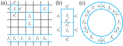
Figure 1: (a) Illustration of elements of $\mathcal{B}^{1}$ in a periodic $6\times 6$ square lattice. When a chain has only one square, e.g., $f_{1}$, its boundary is the four surrounding edges (labeled by blue solid lines). (b) When a chain contains $f_{3}$ and $f_{4}$, the common edge (labeled by blue dashed line) shared by them is not included in the boundary since $e_{3}^{d}\!+\!e_{4}^{u}=0$. (c) When a set of squares ($f_{5}$ to $f_{10}$) forms a row in the lattice, they constitute a ring on the surface.

Since there are a total of $n^{2}$ squares in the lattice, the number of all square chains is $\sum_{i=0}^{n^{2}}C(n^{2},i)=2^{n^{2}}$, where $C(n^{2},i)$ is the number of $i$-combinations from the given $n^{2}$ squares. It is worthwhile to note that the boundary of the square chain which consists of all the $n^{2}$ squares is empty. Explicitly, we have the relation $\partial^{2}(\sum_{i=1}^{n^{2}}f_{i})=0$, where $\partial^{2}$ is the boundary operator which projects a square chain to its boundary. This relation implies that the order of $\mathcal{B}^{1}$ is half of $\sum_{i=0}^{n^{2}}C(n^{2},i)$, which is $2^{n^{2}-1}$.

It is obvious that each element of $\mathcal{B}^{1}$ is a circle in the lattice. In fact, all the circles in the lattice can be divided into four kinds of topological equivalence classes: the topologically trivial circles that are boundaries of some faces; the circles that surround the “handle” of the torus; the ones that encircle the genus of the torus; the ones that surround both the “handle” and the genus. Apparently, the elements of $\mathcal{B}^{1}$ belong to the topologically trivial equivalence classes.

III Topological dynamical decoupling

The physical model that we consider is a set of qubits interacting with their environment. The corresponding total Hamiltonian of the full quantum system reads $H_{t}=H_{S}+H_{E}+H_{S\!E}$, where $H_{S}$ is the qubits’ Hamiltonian, $H_{E}$ is the environment Hamiltonian, and $H_{S\!E}=\sum_{i}\sigma_{\alpha}^{i}\otimes E^{i}$ [$\sigma_{\alpha}^{i}$ and $E^{i}$ are the Pauli-$\alpha$ ($\alpha=x,y$, or $z$) operator acting on the $i$th qubit and its corresponding environment operator, respectively] is the interaction between them. Dynamical decoupling can remove $H_{S\!E}$ from the dynamics of the qubits with fast and strong pulses viola98 ; viola99 . A typical decoupling procedure is composed of repetitive segments, each of which can be described with a notation $[g_{m}^{\dagger},\tau,g_{m}g_{m-1}^{\dagger},\cdots,g_{3}g_{2}^{\dagger},\tau,g_{2}g_{1}^{\dagger},\tau,g_{1}]$, where $g_{i}$ are unitary operators generated by the control pulses. From right to left, this notation means that, apply $g_{1}$ to the qubits, let the system evolve freely for time $\tau$, then apply $g_{2}g_{1}^{\dagger}$ followed by another free evolution for time $\tau$ and so on. A decoupling group is formed when $g_{i}$ form a finite group $\mathcal{G}=\{g_{1},g_{2},\cdots,g_{m}\}$. Let the time scale associated with one such segment be $T_{c}$. In the ideal limit of an arbitrarily short $T_{c}$, the dynamics of the qubits is transformed through a dynamically averaged operator of the form

$$\prod_{\mathcal{G}}(A)=\frac{1}{|\mathcal{G}|}\sum_{i}g_{i}^{\dagger}Ag_{i},$$ (1)

where $|\mathcal{G}|$ is the order of group $\mathcal{G}$, and $A$ is an arbitrary operator acting on $S$ viola99 . It is clear that if a proper group is chosen so that $\prod_{\mathcal{G}}(\sigma_{\alpha}^{i})=0$ for all $i$, the errors caused by $H_{S\!E}$ can be eliminated.

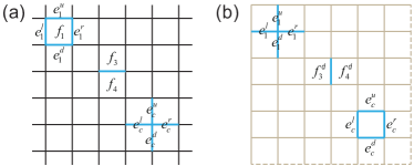
Figure 2: A periodic square lattice (a) and its dual (b). (a) The four edges ($e_{1}^{u}$, $e_{1}^{l}$, $e_{1}^{d}$, and $e_{1}^{r}$) connecting head-to-tail form the boundary of $f_{1}$. The four edges ($e_{c}^{u}$, $e_{c}^{l}$, $e_{c}^{d}$, and $e_{c}^{r}$) sharing the same vertex constitute a cross. (b) The square $f_{1}$ in the original lattice is transformed into a cross in the dual. Meanwhile, a cross in the original lattice is changed into a square in the dual.

Now we show how to remove $H_{S\!E}$ from the dynamics of the qubits. We first define $\mathcal{B}^{z}$. The elements of $\mathcal{B}^{1}$ and those of $\mathcal{B}^{z}$ are in a one-to-one correspondence. An element of $\mathcal{B}^{1}$ contains some edges in the lattice and every edge supports a qubit. An element $b^{1}_{i}\in\mathcal{B}^{1}$ can be transformed into its related element $b^{z}_{i}\in\mathcal{B}^{z}$ by replacing each edge of $b^{1}_{i}$ with the $\sigma_{z}$ operator acting on the corresponding qubit. In this way, $b^{z}_{i}$ turn out to be unitary operators which are strings of Pauli-$Z$ operators on different qubits.

Group $\mathcal{B}^{x}$ is defined on the dual lattice shown in Fig. 2(b). The dual lattice is constructed by placing a vertex within each face, and connecting pairs of these vertices with an edge wherever the two corresponding faces have overlapping boundaries. Each vertex of the original (or primal) lattice then corresponds to the face in the dual lattice whose boundary edges surround it. As we did for the original lattice, we can construct a group $\mathcal{B}^{1d}$ whose elements are the boundaries of the square chains in the dual lattice. Based on $\mathcal{B}^{1d}$, we can define a group $\mathcal{B}^{x}$ whose elements are in a one-to-one correspondence with $\mathcal{B}^{1d}$’s elements. An element $b^{x}_{i}\in\mathcal{B}^{x}$ can be obtained from its related element $b^{1d}_{i}\in\mathcal{B}^{1d}$ by replacing each edge of $b^{1d}_{i}$ with the $\sigma_{x}$ operator acting on the related qubit.

By using $\mathcal{B}^{xz}=\mathcal{B}^{x}\times\mathcal{B}^{z}$ as the decoupling group, we can eliminate local Hamiltonians (such as all $\sigma_{\alpha}^{i}$) from the dynamics with the decoupling procedure denoted by $[b_{2^{2n^{2}-2}}^{xz},\tau,b_{2^{2n^{2}-2}}^{xz}b_{2^{2n^{2}-2}-1}^{xz},\cdots,b^{xz}_{3}b_{2}^{xz},\tau,b^{xz}_{2}b^{xz}_{1},\tau,b^{xz}_{1}]$, where $b^{xz}_{i}$ are the elements in group $\mathcal{B}^{xz}$. The reason is that group $\mathcal{B}^{xz}$ is an Abelian group, thus it has a total of $2^{2n^{2}-2}$ irreducible representations (irreps), each of which is 1-dimensional. The corresponding group algebra takes the form of

$$\mathbb{C}\mathcal{B}^{xz}\cong\oplus_{J=1}^{2^{2n^{2}-2}}M_{d_{J}},$$ (2)

where $J$ is the irrep index, $d_{J}=1$ is the dimension of each irrep. Due to the symmetry of the generators, the Hilbert space $\mathcal{H}$ spanned by the qubits can be decomposed into

$$\mathcal{H}\cong\oplus_{J=1}^{2^{2n^{2}-2}}\mathbb{C}_{n_{J}}\otimes\mathbb{C}_{d_{J}},$$ (3)

where all $n_{J}=4$ and $d_{J}=1$. The $n_{J}=4$ corresponds to the homology degrees of freedom. Therefore, the DD procedure denoted by $[b_{2^{2n^{2}-2}}^{xz},\tau,b_{2^{2n^{2}-2}}^{xz}b_{2^{2n^{2}-2}-1}^{xz},\cdots,b^{xz}_{3}b_{2}^{xz},\tau,b^{xz}_{2}b^{xz}_{1},\tau,b^{xz}_{1}]$ can filter out all the Hamiltonians that have no component in the $\mathbb{C}_{n_{J}}$ section according to the dynamically averaged operator $\prod_{\mathcal{B}^{xz}}(A)$. Apparently, a local Hamiltonian $H$ acting on the qubits, e.g., the single particle Hamiltonians and two-qubit interactions, has no component in $\mathbb{C}_{n_{J}}$, and thus $\prod_{\mathcal{B}^{xz}}(H)=0$. As a result, the linearly independent interaction $H_{I}=\sum_{i,\alpha}\sigma_{\alpha}^{i}\otimes E_{\alpha}^{i}$ ($i$ is the qubit index and $\alpha=x,y,z$) between the qubits and the environment can be removed from the dynamics of the qubits.

Figure 3: (a) A pair of nearest-neighbor qubits $a$ and $b$ (labeled as red circles), and related squares. Qubit $a$ is on the common edge of $f_{1}$ and $f_{2}$ while qubit $b$ is on the common edge of $f_{1}$ and $f_{3}$. (b) Four cases where the corresponding elements in $\mathcal{B}^{z}$ are not commutative with $H_{ab}$.

In addition to the interaction $H_{I}$, our topological DD scheme can also remove the nearest-neighbour interactions between qubits. This is quite relevant to quantum error correction because the unwanted interactions between qubits can spread errors from one qubit to another. Since the error spread can cause undetectable errors, the elimination of the unwanted interactions can help to keep the errors local so that the undetectable errors are avoided.

Now we consider a pair of nearest-neighbor qubits $a$ and $b$ with a Heisenberg interaction $H_{ab}=\sum_{i=x,y,z}\sigma_{i}^{a}\sigma_{i}^{b}$ between them. Among all the elements of $\mathcal{B}^{z}$, there are four kinds of elements that are not commutative with $H_{ab}$: those associated with $f_{2}$ but not $f_{1}$ and $f_{3}$; those associated with $f_{3}$ but not $f_{1}$ and $f_{2}$; those associated with $f_{1}$ and $f_{2}$ but not $f_{3}$; those associated with $f_{1}$ and $f_{3}$ but not $f_{2}$ (see Fig. 3). The number of the elements for every kind is $2^{n^{2}-4}$. Thus, there are a total of $4\times 2^{n^{2}-4}=2^{n^{2}-2}$ elements that are not commutative with $H_{ab}$, which transform $H_{ab}$ into $-\sigma_{x}^{a}\sigma_{x}^{b}-\sigma_{y}^{a}\sigma_{y}^{b}+\sigma_{z}^{a}\sigma_{z}^{b}$. Since the other $2^{n^{2}-2}$ elements leave $H_{ab}$ unchanged, we obtain the averaged operator: $\prod_{\mathcal{B}^{z}}(H_{ab})=\sum_{i=1}^{2n^{2}}\sigma_{z}^{a}\sigma_{z}^{b}$. The remaining terms can be wiped out by the group $\mathcal{B}^{x}$ because half of its elements are commutative with $\prod_{\mathcal{B}^{z}}(H_{ab})$ while the others are not, indicating the same situation as above.

Despite the significant decoupling power, the required steps in the above procedure scale exponentially with the number of the squares. This may limit its practical application. However, if only $H_{S\!E}$ and nearest-neighbor two-qubit interactions $H_{a,b}=\sigma_{\alpha_{a}}^{a}\otimes\sigma_{\alpha_{b}}^{b}$ ($a$, $b$ are the qubit indexes and $\alpha_{a},\alpha_{b}=x,y,z$) are relevant, a much simpler scheme can be developed.

To this end, we introduce two decoupling groups $\mathcal{T}^{z}$ and $\mathcal{T}^{x}$. Explicitly, $\mathcal{T}^{z}=\{I,t_{1},t_{2},t_{1}t_{2}\}$ and $\mathcal{T}^{x}=\{I,t_{1}^{d},t_{2}^{d},t_{1}^{d}t_{2}^{d}\}$, where $t_{1}$ ($t_{1}^{d}$) is a Pauli operator chain which comprises the $\sigma_{z}$ ($\sigma_{x}$) operators acting on all the qubits attached on the vertical edges in the original (dual) lattice, and $t_{2}$ ($t_{2}^{d}$) comprises the $\sigma_{z}$ ($\sigma_{x}$) operators acting on all the qubits attached on the horizontal edges in the original (dual) lattice. The topological meaning of the decoupling groups $\mathcal{T}^{z}$ and $\mathcal{T}^{x}$ is clear. The four elements in group $\mathcal{T}^{z}$ ($\mathcal{T}^{x}$) are related to the topologically trivial circles, the circles surrounding the “handle”, the circles encircling the genus, and the circles surrounding both the “handle” and the genus in the original (dual) lattice, respectively.

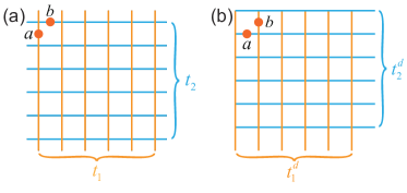
Figure 4: (a) Schematic diagram for the group element $t_{1}$ and $t_{2}$ in the original lattice. (b) Schematic diagram for the corresponding group element $t_{1}^{d}$ and $t_{2}^{d}$ in the dual lattice.

Based on $\mathcal{T}^{z}$, we can design a decoupling procedure $D^{z}=[t_{1}t_{2},\tau,t_{1},\tau,t_{2}t_{1},\tau,t_{1},\tau,I]$, in which $t_{i}\cdot t_{i}=I$ ($i=1,2$) is used. The corresponding dynamically averaged operator for $H_{S\!E}$ can be written as

$$H_{{D}^{z}}=\prod_{\mathcal{T}^{z}}(H_{S\!E})=\sum_{i=1}^{2n^{2}}\sigma_{z}^{i}\otimes E_{z}^{i},$$ (4)

because each qubit on the lattice are associated with two elements in $\mathcal{T}^{z}$ which turn $\sigma_{x}^{a}\otimes E_{x}^{a}+\sigma_{y}^{a}\otimes E_{y}^{a}+\sigma_{z}^{a}\otimes E_{z}^{a}$ into $-\sigma_{x}^{a}\otimes E_{x}^{a}-\sigma_{y}^{a}\otimes E_{y}^{a}+\sigma_{z}^{a}\otimes E_{z}^{a}$ while the other two elements leave it unchanged.

Further, based on $\mathcal{T}^{x}$, a decoupling procedure, ${D}^{xz}=[t_{1}^{d}t_{2}^{d},{D}^{z},t_{1}^{d},{D}^{z},t_{2}^{d}t_{1}^{d},{D}^{z},t_{1}^{d},{D}^{z},I]$ can be established. With ${D}^{xz}$, $H_{S\!E}$ can be removed from the dynamics of the qubits since

$$H_{{D}^{xz}}=\prod_{{\mathcal{T}}^{x}}(H_{{D}^{z}})=0,$$ (5)

for the same reason as $H_{{D}^{z}}$.

Besides $H_{S\!E}$, the nearest-neighbor interaction $H_{a,b}$ between two qubits can be decoupled too. The key point is that, as shown in Fig. 4, qubit $a$ is related to $t_{1}$ ($t_{2}^{d}$) and qubit $b$ is associated with $t_{2}$ ($t_{1}^{d}$) in the original (dual) lattice. It is easy to check that, just like $H_{S\!E}$, $H_{a,b}$ commutes with two elements but anti-commutes with the other two elements in $\mathcal{T}^{z}$ ($\mathcal{T}^{x}$). Therefore, we can obtain

$$\prod_{\mathcal{T}^{x}}(\prod_{\mathcal{T}^{z}}(H_{a,b}))=0,$$ (6)

for any pair of nearest-neighbor $a$ and $b$.

So far, our decoupling procedures are designed based on the original and dual lattices embedded in a torus (with genus $G=1$). A closed surface with a higher genus $G=k$, can be obtained by gluing $k$ tori together. It follows that the corresponding $\mathcal{B}^{z}$ and $\mathcal{B}^{x}$ are $k2^{n^{2}-1}$ ordered groups while $T^{z}$ and $T^{x}$ both have $4k$ elements. Therefore, the decoupling groups on such a surface can be defined and similar decoupling procedures can be developed.

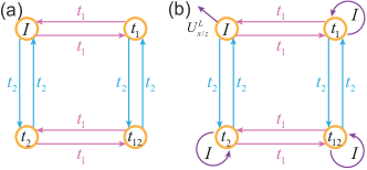
Figure 5: (a) Cayley graph and Eulerian cycles for $\mathcal{T}^{z}$. One possible Eulerian cycle is $I\rightarrow t_{1}\rightarrow t_{12}\rightarrow t_{2}\rightarrow I\rightarrow t_{2}\rightarrow t_{12}\rightarrow t_{1}\rightarrow I$. (b) A modified Eulerian cycle and its Cayley graph to implement logical Pauli-$x$ and Pauli-$z$ operators. Three additional $I$ operators along with a logical operator generated with the same Hamiltonian are added to the original Eulerian cycles.

IV Realizing $D^{z}$ with bounded-strength controls

In the above section, the decoupling procedure $D^{z}$ is developed by assuming the decoupling operators $t_{1}$ and $t_{2}$ can be achieved instantaneously. This requires the capability of applying arbitrarily strong control Hamiltonians, which is not practical in experiments. Below, we show that the same effective Hamiltonian $H_{D^{z}}$ can be realized with bounded-strength controls.

Our method is to use Eulerian cycles on the Cayley graph viola03 associated with group $\mathcal{T}^{z}$ (see Fig. 5). Since $\mathcal{T}^{z}$ consists of two generators $t_{1}$ and $t_{2}$, the corresponding Eulerian cycles comprise $8$ directed edges. One of the possible control paths can be written as $I\xrightarrow{t_{1}}t_{1}\xrightarrow{t_{2}}t_{12}\xrightarrow{t_{1}}t_{2}\xrightarrow{t_{2}}I\xrightarrow{t_{2}}t_{2}\xrightarrow{t_{1}}t_{12}\xrightarrow{t_{2}}t_{1}\xrightarrow{t_{1}}I$ [see Fig. 5(a)], where the time interval between two adjacent decoupling operators is $\tau$. Note that each decoupling operator in the path is related with its former one with a generator ($t_{1}$ or $t_{2}$), implying that we only have to repeatedly applying the generators in the time interval $\tau$ to the qubits according to the control path. It follows that the needed control Hamiltonian for $t_{1}$ or $t_{2}$ can be written as $H_{i}^{z}=\frac{\pi}{2\tau}\sum_{k\in S_{i}}\sigma_{z}^{k}$, where $S_{i}$ being the set of qubits related with $t_{i}$. It is clear that when $\tau$ is nonzero, $H_{1}^{z}$ and $H_{2}^{z}$ are bounded-strength controls. The associated dynamically averaged Hamiltonian $H^{E}_{D^{z}}$ is identical with $H_{D^{z}}$. It follows that if $H_{SE}$ consists of only $\sigma_{x/y}\otimes B_{x/y}$ terms, it can be fully decoupled from the total dynamics.

Given the same assumption, Eulerian cycles based on a modified Cayley graph allow us to build logical gates which are protected by the decoupling procedure [see Fig. 5(b)]. The key idea is that when a particular logical gate $U^{L}$ can be constructed with a Hamiltonian $H^{L}(t)$, we can also obtain an identity with use of $H^{L}$ and with the same error as $U^{L}$ kho09 ; kho09pra . Thus, by adding an identity to each vertex in the Cayley graph (except the one for $U^{L}$), the error caused by $H_{S\!E}$ is averaged by group $\mathcal{T}^{z}$, leaving a net operator $U^{L}$ acting on the qubits. Given a square lattice, there are two logical qubits that can be encoded. The corresponding logical $\sigma_{z}$ and logical $\sigma_{x}$ operators can be constructed with the modified Eulerian cycles [shown in Fig. 5(b)].

We generalize the above idea to realize the procedure $D^{xz}$ whose Cayley graph has 16 vertices with an Eulerian cycle consisting of 64 edges (see Supplemental Materials). Higher order errors can also be eliminated by combining this idea with concatenated DD kh05 ; kh10 ; west10 , so that the procedure can be implemented for long time decoupling.

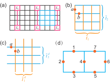
Figure 6: (a) A finite planar square lattice to implement surface codes. Each logical qubit is characterised by a pair of pink squares. When a logical operation on $L_{1}$ is performing, the physical qubits on the small lattice colored blue could be “idle” qubits. (b) The “idle” lattice shown in (a). The red solid circles on the edges are qubits $a$ and $b$, respectively. (c) The dual lattice of the $3\times 3$ lattice in (b). (d) The $1\times 2$ lattice considered in the numerical simulations.

V Application to surface codes

In the above discussion, we focus on the case where the qubits are arranged on a periodic square lattice. Our method can be directly generalized to the case where the qubits are placed on a finite planar square lattice (i.e., a planar lattice with boundaries) shown in Fig. 6(a). This is exactly the same lattice used to implement surface codes fowler12pra .

In doing quantum computation with surface codes, the qubits belonging to some logical qubits (e.g., $L_{1}$) are manipulated while the qubits in the rest area of the lattice, e.g., the qubits labeled blue in Fig. 6(a), have to wait until a certain logical gate is performed. This leaves the “idle” qubits interacting with the environment for a considerable long time, which can cause severe decoherence that may not be correctable stephens14 . Besides, unwanted interactions between qubits can spread errors from one qubit to another, reducing the fault-tolerance of surface codes. Therefore, a method that can suppress the environmental noises on the “idle” qubits, remove the unwanted interactions from the qubits’ dynamics is strongly desired.

This task can be fulfilled by introducing two similar decoupling groups $\tilde{\mathcal{T}}^{z}$ and $\tilde{\mathcal{T}}^{x}$. Here, $\tilde{\mathcal{T}}^{z}=\{I,\tilde{t}_{1},\tilde{t}_{2},\tilde{t}_{1}\tilde{t}_{2}\}$ and $\tilde{\mathcal{T}}^{x}=\{I,\tilde{t}_{1}^{d},\tilde{t}_{2}^{d},\tilde{t}_{1}^{d}\tilde{t}_{2}^{d}\}$, where $I$ is the identity of the qubits, $\tilde{t}_{1}$ ($\tilde{t}_{1}^{d}$) consists of the $\sigma_{z}$ ($\sigma_{x}$) operators acting on all the qubits attached on the vertical edges in the original (dual) lattice, and $\tilde{t}_{2}$ ($\tilde{t}_{2}^{d}$) comprises the $\sigma_{z}$ ($\sigma_{x}$) operators acting on the qubits attached on the horizontal edges in the original (dual) lattice.

Similarly, we can define two procedures $\tilde{D}^{z}=[\tilde{t}_{1}\tilde{t}_{2},\tau,\tilde{t}_{1},\tau,\tilde{t}_{2}\tilde{t}_{1},\tau,\tilde{t}_{1},\tau,I]$ and $\tilde{D}^{xz}=[\tilde{t}_{1}^{d}\tilde{t}_{2}^{d},\tilde{D}^{z},\tilde{t}_{1}^{d},\tilde{D}^{z},\tilde{t}_{2}^{d}\tilde{t}_{1}^{d},\tilde{D}^{z},\tilde{t}_{1}^{d},\tilde{D}^{z},I]$ based on $\tilde{\mathcal{T}}^{z}$ and $\tilde{\mathcal{T}}^{x}$. Based on $\tilde{\mathcal{T}}^{z}$, we develop a decoupling procedure $\tilde{D}^{z}=[\tilde{t}_{1}\tilde{t}_{2},\tau,\tilde{t}_{1},\tau,\tilde{t}_{2}\tilde{t}_{1},\tau,\tilde{t}_{1},\tau,I]$. For a qubit on the lattice [e.g., qubit $a$ in Fig. 6(b)], it is contained only in $\tilde{t}_{1}$ and $\tilde{t}_{1}\tilde{t}_{2}$. It follows that the interaction $H_{S\!E}^{a}$ between qubit $a$ and its environment is modified to $\prod_{\tilde{\mathcal{T}}^{z}}(H_{S\!E}^{a})=\sigma_{z}^{a}\otimes E_{z}^{a}$. Thus

$$H_{\tilde{D}^{z}}=\prod_{\tilde{\mathcal{T}}^{z}}(H_{S\!E})=\sum_{i=1}^{2(n^{2}+n)}\sigma_{z}^{i}\otimes E_{z}^{i}.$$ (7)

After another decoupling procedure $\tilde{D}^{xz}=[\tilde{t}_{1}^{d}\tilde{t}_{2}^{d},\tilde{D}^{z},\tilde{t}_{1}^{d},\tilde{D}^{z},\tilde{t}_{2}^{d}\tilde{t}_{1}^{d},\tilde{D}^{z},\tilde{t}_{1}^{d},\tilde{D}^{z},I]$ based on $\tilde{\mathcal{T}}^{x}$, $H_{S\!E}$ can be completely decoupled since each remaining $\sigma_{z}^{i}\otimes E_{z}^{i}$ term is anti-commutative with two elements (one is $\tilde{t}_{1}^{d}$ or $\tilde{t}_{2}^{d}$, the other is $\tilde{t}_{1}^{d}\tilde{t}_{2}^{d}$) in $\tilde{\mathcal{T}}^{x}$.

From Fig. 6(b) and (c) we observe that a pair of nearest-neighbor qubits $a$ and $b$ is always associated with $\tilde{t}_{1}$ ($\tilde{t}_{2}^{d}$) and $\tilde{t}_{2}$ ($\tilde{t}_{1}^{d}$) in the original (dual) lattice, respectively. This is the same case as we meet in the periodic lattice. Thus, the point there is also valid: $H_{a,b}$ commutes with two elements but anti-commutes with the other two elements in $\tilde{\mathcal{T}}^{z}$ ($\tilde{\mathcal{T}}^{x}$), implying the same result $\prod_{\tilde{\mathcal{T}}^{x}}(\prod_{\tilde{\mathcal{T}}^{z}}(H_{a,b}))=0$.

VI Numerical simulations

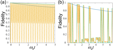
Figure 7: Fidelities between the initial state $|\psi^{L}\rangle$ and the corresponding $\rho(t)$ obtained from the reduced dynamics related to $D^{z}$ or $D^{xz}$ versus evolution time. For each procedure, we consider three cases: (i) with no control Hamiltonian (blue curves), (ii) with bounded-strength control Hamiltonians (yellow curves), and (iii) with arbitrary-strong control Hamiltonians (green curves). (a) Fidelities for $D^{z}$. (b) Fidelities for $D^{xz}$.

To show the validity of our scheme, we perform numerical simulations to calculate the fidelities between an initial logical state and its corresponding one obtained from the reduced dynamics (with or without the dynamical decoupling). Here we consider a $1\times 2$ lattice, which consists of $7$ qubits [see Fig. 6(d)]. The environment interacting with the qubits is described by a set of boson models (i.e., $H_{E}=\sum_{l}\omega_{l}a_{l}^{\dagger}a_{l}$), through the interaction Hamiltonian $H_{S\!E}=\sum_{k,l}\sigma_{\alpha}^{k}(g_{l}^{k}a_{l}+g_{l}^{k*}a_{l}^{\dagger})$, where $a_{l}$ ($a_{l}^{\dagger}$) is the annihilation (creation) operator for the boson model of frequency $\omega_{l}$, and $|g_{l}^{k}|$ correspond to the strength of the interaction, ranging from $0.01\omega_{0}$ to $0.03\omega_{0}$. The Hamiltonian for the total system takes the form

$$H=\sum_{(a,b)\in\mathcal{I}}\omega_{a,b}H_{a,b}+H_{E}+\sum_{k=1}^{7}\sum_{l}\sigma_{\alpha}^{k}(g_{l}^{k}a_{l}+g_{l}^{k*}a_{l}^{{\dagger}}),$$ (8)

where $\mathcal{I}$ is the set of nearest-neighbor qubit pairs [such as ($1,2$), ($2,3$), ($3,4$), and ($4,1$)], $\omega_{a,b}$ is the strength of $H_{a,b}$.

Based on the stabilizers defined on the lattice, the logical state can be chosen as

$$|\psi^{L}\rangle=\frac{1}{2}(|0000000\rangle+|1111000\rangle+|0001111\rangle+|1110111\rangle).$$ (9)

To show the decoupling procedure clearly, we first define the following decoupling operators involved in groups $\tilde{\mathcal{T}}^{z}$ and $\tilde{\mathcal{T}}^{x}$:

$$\tilde{t}_{1}=\sigma_{z}^{2}\sigma_{z}^{4}\sigma_{z}^{6},\tilde{t}_{2}=\sigma_{z}^{1}\sigma_{z}^{3}\sigma_{z}^{5}\sigma_{z}^{7},\tilde{t}_{1}\tilde{t}_{2}=\sigma_{z}^{1}\sigma_{z}^{2}\sigma_{z}^{3}\sigma_{z}^{4}\sigma_{z}^{5}\sigma_{z}^{6}\sigma_{z}^{7};$$

$$\tilde{t}_{1}^{d}=\sigma_{x}^{1}\sigma_{x}^{3}\sigma_{x}^{5}\sigma_{x}^{7},\tilde{t}_{2}^{d}=\sigma_{z}^{2}\sigma_{z}^{4}\sigma_{z}^{6},\tilde{t}_{1}^{d}\tilde{t}_{2}^{d}=\sigma_{x}^{1}\sigma_{x}^{2}\sigma_{x}^{3}\sigma_{x}^{4}\sigma_{x}^{5}\sigma_{x}^{6}\sigma_{x}^{7}.$$ (10)

When $H_{SE}$ consists of only $\sigma_{x}$ and $\sigma_{y}$ terms, it can be removed from the dynamics of the qubits with decoupling group $\mathcal{T}^{z}$. In the first simulation, we choose that qubits $1$ to $4$ couple to the environment with $\sigma_{x}$ and qubits $5$ to $7$ couple to the environment with $\sigma_{y}$, the time interval between two pulses to be $\tau=0.1\omega_{0}t$ and all $\omega_{a,b}=0$. We consider three cases: (i) free evolution without control, (ii) realizing $D^{z}$ with arbitrarily strong controls, (iii) realizing $D^{z}$ with bounded-strength controls. The results have been shown in Fig. 7(a). One may notice that the fidelity for case (iii) fluctuates with time. This is because the initial state $|\psi^{L}\rangle$ is an eigenstate of the decoupling operators, but not an eigenstate of the control Hamiltonians $H_{1}^{z}$ and $H_{2}^{z}$.

When $H_{SE}$ comprises $\sigma_{x}$, $\sigma_{y}$, and $\sigma_{z}$ terms at the same time, we need to use $D^{xz}$ as the decoupling procedure. In this case, the qubits interact with the environment through Pauli operators randomly. In this simulation, we also set $\tau=0.1\omega_{0}t$. Under this condition, $D^{xz}$ can be realized with bounded-strength controls based on Eulerian cycles (for details, see Supplemental Materials). Here, we also set all $\omega_{a,b}=0$ and consider three cases: (i) free evolution without control, (ii) realizing $D^{xz}$ with arbitrarily strong controls, (iii) realizing $D^{xz}$ with bounded-strength controls. The results have been shown in Fig. 7(b).

We also consider a case where $\omega_{a,b}$ are set to be $0.03\omega_{0}$ (i.e., the interactions between nearest-neighbor qubits are open) and $H_{SE}$ consists of only $\sigma_{x}$ and $\sigma_{y}$ terms. By using $D^{z}$ and its related Eulerian cycles (setting $\tau=0.1\omega_{0}t$), we consider three cases: (i) free evolution without control, (ii) realizing $D^{z}$ with arbitrarily strong controls, (iii) realizing $D^{z}$ with bounded-strength controls. The results are shown in Fig. 8.

The reduced dynamics of the qubits can be obtained by using the stochastic Liouville equation methods sto97 ; sto02 ; koch08 ; yan16 . We choose a Lorenz type spectrum $J(\omega)=\gamma/(\gamma^{2}+\omega^{2})$ without the Matsubara terms, where $\gamma$ is the inverse of the bath correlation time. The corresponding correlation function is assumed to be of the exponential form $\alpha(t-s)=(\Gamma\gamma/2)\exp(-\gamma|t-s|)$ with $\Gamma$ being the coupling strength to the environment and $\gamma=1$.

The state fidelity is defined as $F(t)=\sqrt{\langle\psi^{L}|\rho(t)|\psi^{L}\rangle}$, where $\rho(t)$ is obtained from the reduced dynamics. In Fig. 7 (a) and (b), fidelities for the decoupling procedure $D^{z}$ and $D^{xz}$ are demonstrated. In order to show the instantaneous dynamics clearly, we choose a relatively long inner-pulse interval $\tau=0.1\omega_{0}t$. Despite this, the numerical results show that our scheme improves the free fidelities considerably. For example, Fig. 7(a) shows that, compared with the final fidelity for the free evolution ($88.2\%$), the final fidelities for the ideal control and the Eulerian cycle increase by $7.8\%$ and $7.6\%$, respectively. With a shorter $\tau$, the fidelities can be improved further. Another significant advantage demonstrated in Fig. 7 is that our scheme does not require arbitrary strong pulses: for $D^{z}$, the final fidelity for the bounded-strength controls is almost identical to the arbitrarily strong ones; for $D^{xz}$, the difference between the final fidelity for the bounded-strength controls and that for the ideal ones is less than $1\%$. This indicates that our scheme can be implemented with practical experimental technology.

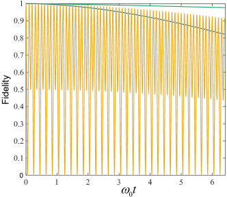
Figure 8: Fidelities between the initial state $|\psi^{L}\rangle$ and the corresponding $\rho(t)$ obtained from the reduced dynamics related to $D^{z}$ with $\omega_{a,b}=0.03\omega_{0}$ versus evolution time. We consider three cases: (i) with no control Hamiltonian (blue curve), (ii) with bounded-strength control Hamiltonians (yellow curve), and (iii) with arbitrarily strong control Hamiltonians (green curve).

VII Conclusions

In summary, we have used topological concepts to develop DD procedures to protect the qubits arranged on square lattices. In each procedure, the decoupling groups are formed from the original lattice and its dual. Owing to the topological nature of the decoupling groups, quantum information stored in the homology degrees of freedom can be preserved. We further show that the designed decoupling procedure can be implemented with realistic strength controls for a long time period. As an example, we explicitly show how our scheme can be generalized to a practical surface code implementation where a planar lattice with boundaries is involved. Our scheme opens a window to introduce DD approach to surface codes so that the errors caused by environments can be reduced, making the required threshold a more easily reachable target.

- (1) D. P. DiVincenzo, Quantum computation, Science 270, 255 (1995).
- (2) A. Ekert and R. Josza, Quantum computation and Shor’s factoring algorithm, Rev. Mod. Phys. 68, 733 (1996).
- (3) P. W. Shor, Scheme for reducing decoherence in quantum computing memory, Phys. Rev. A 52, R2493 (1995).
- (4) A. M. Steane, Error correcting codes in quantum theory, Phys. Rev. Lett. 77, 793 (1996).
- (5) R. Laflamme, C. Miquel, J. P. Paz, and W. H. Zurek, Perfect quantum error correcting code, Phys. Rev. Lett. 77, 198 (1996).
- (6) B. M. Terhal, Quantum error correction for quantum memories, Rev. Mod. Phys. 87, 307 (2015).
- (7) X.-C. Yao, T.-X. Wang, W.-B. G. Hao-Ze Chen, A. G. Fowler, R. Raussendorf, Z.-B. Chen, N.-L. Liu, C.-Y. Lu, Y.-J. Deng, Y.-A. Chen, and J.-W. Pan, Experimental demonstration of topological error correction, Nature (London) 482, 489 (2012).
- (8) R. Barends, J. Kelly, A. Megrant, A. Veitia, D. Sank, E. Jeffrey, T. C. White, J. Mutus, A. G. Fowler, B. Campbell, Y. Chen, Z. Chen, B. Chiaro, A. Dunsworth, C. Neill, P. O’Malley, P. Roushan, A. Vainsencher, J. Wenner, A. N. Korotkov, A. N. Cleland, and J. M. Martinis, Superconducting quantum circuits at the surface code threshold for fault tolerance, Nature (London) 508, 500 (2014).
- (9) D. Nigg, M. Müller, E. A. Martinez, P. Schindler, M. Hennrich, T. Monz, M. A. Martin-Delgado, and R. Blatt, Quantum computations on a topologically encoded qubit, Science 345, 302 (2014).
- (10) A. D. Corcoles, E. Magesan, S. J. Srinivasan, A. W. Cross, M. Steffen, J. M. Gambetta, and J. M. Chow, Demonstration of a quantum error detection code using a square lattice of four superconducting qubits, Nat. Commun. 6, 6979 (2015).
- (11) J. Kelly, R. Barends, A. G. Fowler, A. Megrant, E. Jeffrey, T. C. White, D. Sank, J. Y. Mutus, B. Campbell, Y. Chen, Z. Chen, B. Chiaro, A. Dunsworth, I.-C. Hoi, C. Neill, P. J. J. O’Malley, C. Quintana, P. Roushan, A. Vainsencher, J. Wenner, A. N. Cleland, and J. M. Martinis, State preservation by repetitive error detection in a superconducting quantum circuit, Nature (London) 519, 66 (2015).
- (12) A. Y. Kitaev, Quantum computations: algorithms and error correction, Russ. Math. Surv. 52, 1191 (1997).
- (13) S. B. Bravyi and A. Y. Kitaev, Quantum codes on a lattice with boundary, arXiv:quant-ph/9811052.
- (14) E. Dennis, A. Y. Kitaev, A. Landahl, and J. Preskill, Topological quantum memory, J. Math. Phys. 43, 4452 (2002).
- (15) A. G. Fowler, M. Mariantoni, J. M. Martinis, and A. N. Cleland, Surface codes: Towards practical large-scale quantum computation, Phys. Rev. A 86, 032324 (2012).
- (16) S. Vijay, T. H. Hsieh, and L. Fu, Majorana Fermion Surface Code for Universal Quantum Computation, Phys. Rev. X 5, 041038 (2015).
- (17) L. A. Landau, S. Plugge, E. Sela, A. Altland, S. M. Albrecht, and R. Egger, Towards Realistic Implementations of a Majorana Surface Code, Phys. Rev. Lett. 116, 050501 (2016).
- (18) B. J. Brown, K. Laubscher, M. K. Kesselring, and J. R. Wootton, Poking Holes and Cutting Corners to Achieve Clifford Gates with the Surface Code, Phys. Rev. X 7, 021029 (2017).
- (19) D. K. Tuckett, S. D. Bartlett, and S. T. Flammia, Ultrahigh Error Threshold for Surface Codes with Biased Noise, Phys. Rev. Lett. 120, 050505 (2018).
- (20) H. Bombin and M. A. Martin-Delgado, Topological quantum distillation, Phys. Rev. Lett. 97, 180501 (2006).
- (21) H. G. Katzgraber, H. Bombin, and M. A. Martin-Delgado, Error Threshold for Color Codes and Random Three-Body Ising Models, Phys. Rev. Lett. 103, 090501 (2009).
- (22) H. Bombin, Gauge color codes: optimal transversal gates and gauge fixing in topological stabilizer codes, New J. Phys. 17, 083002 (2015).
- (23) D. Litinski, M. S. Kesselring, J. Eisert, and F. von Oppen, Combining Topological Hardware and Topological Software: Color-Code Quantum Computing with Topological Superconductor Networks, Phys. Rev. X 7, 031048 (2017).
- (24) Y. Li, Fault-tolerant fermionic quantum computation based on color code, Phys. Rev. A 98, 012336 (2018).
- (25) A. G. Fowler, Proof of Finite Surface Code Threshold for Matching, Phys. Rev. Lett. 109, 180502 (2012).
- (26) A. M. Stephens, Fault-tolerant thresholds for quantum error correction with the surface code, Phys. Rev. A 89, 022321 (2014).
- (27) L. Viola and S. Lloyd, Dynamical suppression of decoherence in two-state quantum systems, Phys. Rev. A 58, 2733 (1998).
- (28) L. Viola, E. Knill, and S. Lloyd, Dynamical decoupling of open quantum systems, Phys. Rev. Lett. 82, 2417 (1999).
- (29) L. Viola, E. Knill, and S. Lloyd, Dynamical generation of noiseless quantum subsystems, Phys. Rev. Lett. 85, 3520 (2000).
- (30) L. Viola and E. Knill, Robust Dynamical Decoupling of Quantum Systems with Bounded Controls, Phys. Rev. Lett. 90, 037901 (2003).
- (31) L. Viola, and E. Knill, Random Decoupling Schemes for Quantum Dynamical Control and Error Suppression, Phys. Rev. Lett. 94, 060502 (2005).
- (32) K. Khodjasteh and D. A. Lidar, Fault-tolerant quantum dynamical decoupling, Phys. Rev. Lett. 95, 180501 (2005).
- (33) K. Khodjasteh, D. A. Lidar, and L. Viola, Arbitrarily accurate dynamical control in open quantum systems, Phys. Rev. Lett. 104, 090501 (2010).
- (34) G. S. Uhrig, Keeping a quantum bit alive by optimized -pulse sequences, Phys. Rev. Lett. 98, 100504 (2007).
- (35) G. Gordon, G. Kurizki, and D. A. Lidar, Optimal Dynamical Decoherence Control of a Qubit, Phys. Rev. Lett. 101, 010403 (2008).
- (36) W. Yang and R. B. Liu, Universality of Uhrig Dynamical Decoupling for Suppressing Qubit Pure Dephasing and Relaxation, Phys. Rev. Lett. 101, 180403 (2008).
- (37) H. Uys, M. J. Biercuk, and J. J. Bollinger, Optimized Noise Filtration through Dynamical Decoupling, Phys. Rev. Lett. 103, 040501 (2009).
- (38) J. R. West, B. H. Fong, and D. A. Lidar, Near-Optimal Dynamical Decoupling of a Qubit, Phys. Rev. Lett. 104, 130501 (2010).
- (39) J. Du, X. Rong, N. Zhao, Y. Wang, J. Yang, and R. B. Liu, Preserving electron spin coherence in solids by optimal dynamical decoupling, Nature (London) 461, 1265 (2009).
- (40) J. Zhang and D. Suter, Experimental protection of two-qubit quantum gates against environmental noise by dynamical decoupling, Phys. Rev. Lett. 115, 110502 (2015).
- (41) F. Wang, C. Zu, L. He, W.-B. Wang, W.-G. Zhang, and L.-M. Duan, Experimental realization of robust dynamical decoupling with bounded controls in a solid-state spin system, Phys. Rev. B 94, 064304 (2016).
- (42) Quantum Error Correction, edited by D. A. Lidar and T. A. Brun (Cambridge University Press, Cambridge, UK, 2013).
- (43) K. Khodjasteh and L. Viola, Dynamically Error-Corrected Gates for Universal Quantum Computation, Phys. Rev. Lett. 102, 080501 (2009).
- (44) K. Khodjasteh and L. Viola, Dynamical quantum error correction of unitary operations with bounded controls, Phys. Rev. A 80, 032314 (2009).
- (45) J. R. West, D. A. Lidar, B. H. Fong, and M. F. Gyure, High Fidelity Quantum Gates via Dynamical Decoupling, Phys. Rev. Lett. 105, 230503 (2010).
- (46) J. T. Stockburger and C. H. Mak, Dynamical simulation of current fluctuations in a dissipative two-state system, Phys. Rev. Lett. 80, 2657 (1998).
- (47) J. T. Stockburger and H. Grabert, Exact c-number Representation of Non-Markovian Quantum Dissipation, Phys. Rev. Lett. 88, 170407 (2002).
- (48) W. Koch and F. Großmann, Non-Markovian dissipative semiclassical dynamics, Phys. Rev. Lett. 100, 230402 (2008).
- (49) Y.-A. Yan and J. Shao, Stochastic description of quantum Brownian dynamics, Front. Phys. 11, 110309 (2016).