Entanglement and thermodynamic entropy in a clean many-body localized system

Abstract

Whether or not the thermodynamic entropy is equal to the entanglement entropy of an eigenstate, is of fundamental interest, and is closely related to the ‘Eigenstate thermalization hypothesis (ETH)’. However, this has never been exploited as a diagnostic tool in many-body localized systems. In this work, we perform this diagnostic test on a clean interacting system (subjected to a static electric field) that exhibits three distinct phases: integrable, non-integrable ergodic and non-integrable many-body-localized (MBL). We find that in the non-integrable phase, the equivalence between the thermodynamic entropy and the entanglement entropy of individual eigenstates, holds. In sharp contrast, in the integrable and non-integrable MBL phases, the entanglement entropy shows large eigenstate-to-eigenstate fluctuations, and differs from the thermodynamic entropy. Thus the non-integrable MBL phase violates ETH similar to an integrable system; however, a key difference is that the magnitude of the entanglement entropy in the MBL phase is significantly smaller than in the integrable phase, where the entanglement entropy is of the same order of magnitude as in the non-integrable phase, but with a lot of eigenstate-to-eigenstate fluctuations. Quench dynamics from an initial CDW state independently supports the validity of the ETH in the ergodic phase and its violation in the MBL phase.

I Introduction

The question of how an isolated many-body system thermalizes has a long history. In the classical domain, thermalization of an isolated system in the limit of long times is governed by Boltzmann’s ergodic hypothesis (Huang, 2009; Pathria and Beale, 2011; Penrose, 1979). It states that classical chaotic systems, uniformly sample all the available micro-states at a given energy, in the long time limit. However, this hypothesis cannot be generalized directly to the quantum domain as in the long time limit the expectation value of an observable retains the initial memory of the system, and is thus unable to sample all the eigenstates of the system. Experimental advancement Kinoshita et al. (2006); Hofferberth et al. (2007); Rigol et al. (2008) in recent times has created a strong demand for a close understanding of thermalization in isolated quantum systems and led to a flurry of theoretical activity (Rigol, 2009; Santos and Rigol, 2010a; Rigol and Fitzpatrick, 2011; He and Rigol, 2012; Mondaini and Rigol, 2015; Beugeling et al., 2014a; Rigol et al., 2007; Santos and Rigol, 2010b; Canovi et al., 2011; Rigol and Santos, 2010).

Thermodynamic entropy in the context of classical statistical mechanics is by its very nature an extensive quantity (Huang, 2009; Penrose, 1979; Pathria and Beale, 2011). In quantum systems, entanglement entropy of individual eigenstates brings in a rich additional dimension. Discussions of the extensivity or the lack thereof of entanglement entropy have abounded (Vitagliano et al., 2010; Wolf, 2006; Lai et al., 2013; Roy and Sharma, 2018; Roy et al., 2019; Pouranvari and Yang, 2014) in recent times. The celebrated area law (Hastings, 2007; Laflorencie, 2016; Eisert et al., 2010) which asserts that the ground state entanglement entropy scales with subsystem as the surface area of the subsystem, has been a central topic around which many of these studies have been carried out. However, the relationship between entanglement entropy and thermodynamic entropy has only been scantily covered Deutsch et al. (2013). In this Letter, we demonstrate, with the aid of a specific example, that a systematic study of this relationship is an illuminating diagnostic for a class of quantum phase transitions.

For an isolated quantum system it has been argued that the route to thermalization is described by the eigenstate thermalization hypothesis(ETH)(Deutsch, 1991; Srednicki, 1994; Rigol et al., 2008; Deutsch, 2018; D’Alessio et al., 2016). The ETH states that expectation values of operators in the eigenstates of the Hamiltonian are identical to the their thermal values, in the thermodynamic limit. The measurement of any local observable in these systems gives the same expectation values for nearby energies. A closely related, but completely independent feature analogous to the ETH is the question of whether the thermodynamic entropy of a subsystem obtained from the micro-canonical reduced density matrix with a fixed energy $E_{0}$ is equal to the entanglement entropy calculated from the energy eigenstate of the system with the same energy $E_{0}$ (Deutsch, 2010; Deutsch et al., 2013).

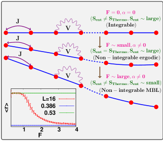
Figure 1: A schematic representation of the model with our main findings. In the non-integrable ergodic phase, the entanglement entropy matches with the thermodynamic entropy, while in the integrable and non-integrable MBL phases, it differs from the thermodynamic entropy. In the non-integrable MBL phase, the magnitude of the entanglement entropy is significantly smaller. The arrow represents the direction of increasing field strength. The inset shows the mean level-spacing ratio (averaged over different values of $\alpha$) as a function of the field strength. The other parameters are: $L=16,V=1.0$ and filling factor $=0.5$.

The phenomenon of many-body localization (MBL) (Gornyi et al., 2005; Basko et al., 2006; Anderson, 1958; Nandkishore and Huse, 2015; Pal and Huse, 2010) in which interactions fail to destroy Anderson localization ( caused by random disorder) has created considerable excitement. The MBL phase is believed to exhibit properties similar to those of integrable systems (Vosk and Altman, 2013; Huse et al., 2014; Vasseur and Moore, 2016; Abanin et al., 2019; Imbrie et al., 2017; Serbyn et al., 2013; Chandran et al., 2015). In particular, although the ETH criterion is known to be satisfied by generic, non-integrable systems (Khatami et al., 2012a; He et al., 2013; Tang et al., 2015; Beugeling et al., 2014b; Santos and Rigol, 2010b; Kim et al., 2014; Santos and Rigol, 2010a; Rigol and Srednicki, 2012; Ikeda et al., 2013), a violation of the ETH is expected for integrable, and therefore MBL systems (Rigol, 2009; Deutsch et al., 2013; Mondaini and Rigol, 2015; Khatami et al., 2012b). The expectation value of any local observable in these systems fluctuates wildly for nearby eigenstates. Integrable systems are exactly solvable and have an extensive number of local conserved currents (Sutherland, 2004), which do not evolve in the course of time and hence, prevent the system from thermalization. Similarly, MBL systems have conserved quasi-local integrals of motion which help to retain the memory of the initial state Abanin et al. (2019); Imbrie et al. (2017); Serbyn et al. (2013); Chandran et al. (2015).

Most MBL systems have in-built disorder (Luitz et al., 2015; Nandkishore and Huse, 2015; Iyer et al., 2013). Recent work (Schulz et al., 2019; van Nieuwenburg et al., 2019) has proposed that a stable MBL-like phase may be obtained in a clean (disorderless) interacting system subjected to an electric field and a confining/disordered potential. The additional potential turns out to be essential as in its absence, the MBL phase cannot be obtained Schulz et al. (2019); van Nieuwenburg et al. (2019); Moudgalya et al. (2019); Taylor et al. (2019). This many-body system is known to exhibit a rich phase diagram. In the absence of both electric field and curvature term, this model is integrable, while a finite value of either of these external potentials breaks the integrability. Further in the region of broken integrability it shows a transition from the ergodic to the MBL phase on varying the strength of the electric field. Thus it provides a good test bed to characterize various phases: integrable, non-integrable ergodic and non-integrable MBL phases. As opposed to a standard disordered system, a clean system could potentially be realized experimentally with greater ease, while still using the already available methods (Schreiber et al., 2015; Choi et al., 2016; Smith et al., 2016; Kondov et al., 2015; Bordia et al., 2017).

In this article, we demonstrate the profitability of a study of the relationship between thermodynamic entropy and entanglement entropy to characterize various phases. Although our technique is, in principle, more general, we concentrate on the concrete case of the above disorder-free model. We find that for a small subsystem, the entanglement entropy of each eigenstate matches with the thermodynamic entropy, provided the system is tuned in the non-integrable ergodic phase and satisfies the ETH criterion. However in the integrable and non-integrable MBL phases, the entanglement entropy shows large fluctuations for nearby eigenstates, and also differs from the thermodynamic entropy. The difference between the thermodynamic entropy and the entanglement entropy increases on varying the strength of the electric field due to the strong localization from the electric field which leads to a smaller entanglement entropy. Further tests are done from an alternative perspective by studying the dynamics of average particle number in the subsystem. In the long time limit, the saturation value of the observable in the non-integrable ergodic phase matches with the results predicted by the diagonal ensemble and the microcanonical ensemble, while in the non-integrable MBL phase the saturation value matches with the diagonal ensemble result but differs from the microcanonical ensemble result.

II Model Hamiltonian

We consider the clean, spinless fermionic Hamiltonian with $L$ sites  Schulz et al. (2019):

$$H=-J\sum_{j=0}^{L-2}(c_{j}^{\dagger}c_{j+1}+c_{j+1}^{\dagger}c_{j})-F\sum_{j=0}^{L-1}j(n_{j}-\frac{1}{2})\qquad$$

$$+\alpha\sum_{j=0}^{L-1}\frac{j^{2}}{(L-1)^{2}}(n_{j}-\frac{1}{2})+V\sum_{j=0}^{L-2}(n_{j}-\frac{1}{2})(n_{j+1}-\frac{1}{2}),$$

where $c,c^{\dagger}$ are the fermionic operators, $F$ is the linear electric field, $\alpha$ is the curvature term and $V$ is the nearest neighbor interaction. The form of the curvature term provides a slight non-linearity in the overall onsite potential. The lattice constant is kept at unity and natural units ($J=\hbar=e=1$) are adopted for all the calculations. In the non-interacting limit $(V=0)$ with $\alpha=0$, the above Hamiltonian yields the Wannier-Stark ladder characterized by an equi-spaced energy spectrum proportional to the electric field strength, and where all the single particle eigenstates are localized (Krieger and Iafrate, 1986; Wannier, 1960). Furthermore, the dynamics governed by this Hamiltonian gives rise to oscillatory behavior which is known as Bloch oscillations (Bouchard and Luban, 1995; Mendez and Bastard, 1993; Hartmann et al., 2004; Bhakuni and Sharma, 2018; Bhakuni et al., 2019). When interactions are included, the model is integrable in the absence of both the static field and the curvature term ($F=0,\alpha=0$). The integrability is broken by a non-zero value of either the field $F$ or the curvature $\alpha$. When the field $F$ is varied while keeping $\alpha$ fixed at a non-zero value, the system undergoes a transition from a delocalized (ergodic) phase at small field strengths to the MBL phase (Schulz et al., 2019; van Nieuwenburg et al., 2019) at large field strengths. The inset of Fig. 1 carries a plot of the mean level spacing ratio (Oganesyan and Huse, 2007) (averaged over the curvature parameter $\alpha$) as a function of the field, indicating a change of statistics (Atas et al., 2013) from Wigner-Dyson to Poisson.

III ETH and thermodynamic entropy

For an isolated quantum system described by a Hamiltonian $H$, the time evolution of any initial state is given by

$$|\psi(t)\rangle=e^{-iHt}|\psi(0)\rangle=\sum_{n}c_{n}e^{-i\epsilon_{n}t}|n\rangle,$$ (2)

where $\epsilon_{n}$ and $|n\rangle$ are the eigenvalues and the eigenstates of the Hamiltonian respectively. The information of the initial state is encoded into the coefficients $c_{n}$. For any operator $\hat{\mathcal{O}}$ the expectation value after any time $t$ is given by

$$\langle\hat{\mathcal{O}}(t)\rangle=\langle\psi(t)|\hat{\mathcal{O}}(t)|\psi(t)\rangle.$$ (3)

Using Eq. 2, this simplifies to

$$\langle\hat{\mathcal{O}}(t)\rangle=\sum_{n}|c_{n}|^{2}\mathcal{O}_{nn}+\sum_{m\neq n}c^{*}_{m}c_{n}e^{i(\epsilon_{m}-\epsilon_{n})t}\mathcal{O}_{mn},$$ (4)

where $\mathcal{O}_{mn}$ are the matrix elements of the operator $\hat{\mathcal{O}}$ in the eigenbasis of the Hamiltonian $H$. It can be seen from Eq. 4 that in the long time limit ($t\to\infty$), generically (in the absence of degeneracy) the second term goes to zero and the expectation value of the observable saturates to the value predicted by the diagonal ensemble:

$$\langle\hat{\mathcal{O}}(t\to\infty)\rangle=\langle\hat{\mathcal{O}}_{DE}\rangle=\sum_{n}|c_{n}|^{2}\mathcal{O}_{nn}.$$ (5)

Hence the system retains the memory of the initial state through the coefficients $c_{n}$, and does not follow the ergodic hypothesis.

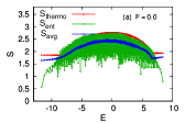
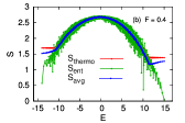
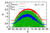
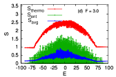
Figure 2: The entanglement entropy of each energy eigenstate and the corresponding thermodynamic entropy. (a) Integrable phase ($F=0$, $\alpha=0$): the entropy of nearby eigenstates fluctuates wildly with a finite difference between average entropy and the microcanonical average. (b,c,d) Non-integrable phase : with $\alpha=1.0$ and $F=0.4,1.5,\ \text{and}\ 3.0$ respectively. We obtain agreement between the entanglement entropy with its corresponding thermodynamic entropy in the ergodic phase $(F=0.4)$ satisfying ETH while the ETH is violated on increasing the value of field strength (going into the MBL phase). The other parameters are: $L=16,V=1.0$ filling factor $=0.5$, and subsystem size $m=4$.

Thermalization in isolated quantum many body systems happens via the mechanism of ETH, which implicitly involves the assumption that the diagonal elements of the operator $\hat{\mathcal{O}}$ change slowly with the eigenstates. Specifically, the off-diagonal elements $\mathcal{O}_{mn}$, and the difference in the neighboring diagonal elements: $\mathcal{O}_{n+1,n+1}-\mathcal{O}_{n,n}$ are exponentially small in $\mathcal{N}$, with $\mathcal{N}$ being the system size. With this assumption, the diagonal ensemble result (Eq. 5) saturates to a constant value as the matrix elements $\mathcal{O}_{nn}$ are effectively constant over a given energy window.

Now considering the micro-canonical ensemble, the average value of the same observable can be written as

$$\langle\hat{\mathcal{O}}_{ME}\rangle=\frac{1}{N_{\text{states}}}\sum_{n=1}^{N_{\text{states}}}\mathcal{O}_{nn},$$ (6)

where $N_{\text{states}}$ is the number of states in a given energy shell. Imposing the assumption of ETH, this also saturates to a constant value. Thus in the long time limit, the system thermalizes and the observable saturates to a thermal value predicted by the micro-canonical ensemble (Rigol et al., 2008; Kim et al., 2014; Rigol and Srednicki, 2012).

Under these conditions the expectation value of the operator $\hat{\mathcal{O}}$ in the energy eigenstate characterized by the density matrix $\rho_{E}\equiv|E\rangle\langle E|$ is the same as the micro-canonical average of the same operator:

$$\text{Tr}(\rho_{E}\hat{\mathcal{O}})=\text{Tr}(\rho_{\text{micro},E}\hat{\mathcal{O}}),$$ (7)

where the microcanonical density matrix is defined as

$$\rho_{\text{micro},E_{0}}=\frac{1}{N_{\text{states}}}\sum_{E_{0}<E<E_{0}+\Delta E}|E\rangle\langle E|,$$ (8)

where $N_{\text{states}}$ is the number of states available in the energy window $\Delta E$.

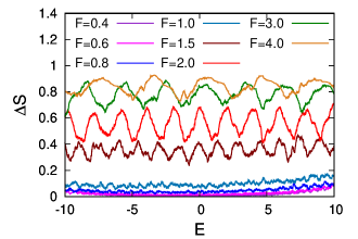
Figure 3: The difference between the thermodynamic entropy and the average entropy as a function of energy. Only the central part of the spectrum ($E\in[-10:10]$) is shown for various values of the field strength. In the ergodic phase the difference is almost zero while in the MBL phase the difference is much larger. The other parameters are: $L=16,\alpha=1.0,V=1.0$ filling factor $=0.5$, and subsystem size $m=4$.

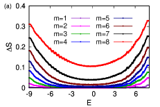
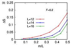
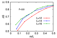
Figure 4: (a) Difference between the thermodynamic entropy and the average entropy (average carried out over $100$ nearest eigenstates in both cases) as a function of energy for different subsystem sizes in the ergodic phase($F=0.2$). A better thermalization can be seen for smaller subsystem sizes. (b,c) The finite size scaling of the difference of thermodynamic and average entropy (for a single eigenstate located at the middle of spectrum) as a function of the subsystem size in both ergodic and MBL phases. The other parameters are: $L=16,\alpha=1.0,V=1.0$ filling factor $=0.5$.

For a composite system $(A+B)$ characterized by the density matrix $\rho$, the entanglement entropy of a subsystem $A$ is defined as: $S_{\text{Ent}}=-\text{Tr}(\rho_{A}\text{ln}\rho_{A})$, where $\rho_{A}=\text{Tr}_{B}\rho$, is the reduced density matrix of the subsystem $A$ taken after tracing out the degrees of freedom of the other subsystem $B$. On the other hand, the thermodynamic entropy from a microcanonical ensemble is defined as: $S_{\text{thermo}}=-\text{Tr}(\rho_{\text{micro}}\text{ln}\rho_{\text{micro}})$. The criterion of ETH is extended (Deutsch et al., 2013; Deutsch, 2010) by asking whether the entanglement entropy of a small subsystem taken out of a large system in an eigenstate with energy $E_{0}$ is equal to the thermodynamic entropy computed from the micro-canonical density matrix (Eq. 8) with the same energy $E_{0}$. Positing an ETH-like equation where $\rho_{\text{micro}}$ is replaced by $\rho_{A}$ we ask if the condition

$$S_{\text{thermo}}=-\text{Tr}(\rho_{A}\text{ln}\rho_{A})=-\text{Tr}(\rho_{A,\text{micro}}\text{ln}\rho_{A,\text{micro}})$$ (9)

holds. Here, $\rho_{A,\text{micro}}$ is the reduced density matrix corresponding to the density matrix $\rho_{\text{micro}}$. For the subsystem $A$, this can be calculated by tracing out the degree of freedom of the remaining part: $\rho_{A,\text{micro}}=\text{Tr}_{B}(\rho_{A,\text{micro}})$.

Although the above criterion is analogous to the standard ETH one (Eq. 7) the logarithmic factor $\text{ln}\rho_{A}$ is not an observable quantity, thus making it an independent characteristic of thermalization.

IV Results and discussion

IV.1 Statics

The model considered contains three regimes of interest: the integrable phase, the non-integrable ergodic phase and the non-integrable MBL phase. We employ numerical exact diagonalization of the model (Eq. II) for a system size upto $L=16$ with the filling factor set to half filling. We also define the subsystem $A$ as consisting of first $m$ sites out of the $L$ sites. We test the equivalence of the thermodynamic entropy and entanglement entropy (Eq. 9) in these distinct phases. We compute the entanglement entropy for a small subsystem ($m=4$) for all the eigenstates and plot it in Fig. 2. The thermodynamic entropy for all the eigenstates is also plotted by considering the microcanonical density matrix (Eq. 8), followed by tracing out the degrees of freedom of the complement of the subsystem. Since the energy spectrum fans out as a function of the electric field strength, we average the density matrix over $N_{\text{states}}=100$ nearest-neighbor eigenstates to compute the thermodynamic entropy. Furthermore, the average entanglement entropy $S_{\text{avg}}$ (average of the entanglement entropy of $100$ nearby eigenstates) is also plotted in the same figure.

In the integrable case ($F,\alpha=0$), the thermodynamic entropy differs from the entanglement entropy with the latter having a lot of fluctuations. However, for the parameters in the ergodic phase, nice agreement is found between the thermodynamic entropy and entanglement entropy, which signifies the validity of ETH in this phase. When the system is tuned on the border ($F=1.5$), the entanglement entropy also shows fluctuations due to a mixture of both volume law and area law scaling states. This in-between phase has been called the “S-phase”  (Xu et al., 2019). For the parameters in the MBL region, the entanglement entropy shows wild fluctuations and the thermodynamic entropy is also different from the entanglement entropy, which suggests the breakdown of ETH in the MBL phase. It is interesting to note that even though both integrable and non-integrable MBL phases violate the ETH, the magnitude of entanglement is considerably lower in the latter, due to the underlying localization.

It is useful to consider the difference between thermodynamic entropy and the average entanglement entropy:

$$\Delta S=\frac{S_{\text{thermo}}-S_{\text{avg}}}{S_{\text{thermo}}}.$$ (10)

The difference between the thermodynamic entropy and the entanglement entropy ($\Delta S$) increases on increasing the electric field strength. The entropy for a part of the spectrum ($E\in[-10:10]$) is plotted in Fig. 3 for various values of the field strengths. In the ergodic phase the difference is close to zero signifying the validity of ETH while a finite difference in the MBL phase shows the violation of ETH.

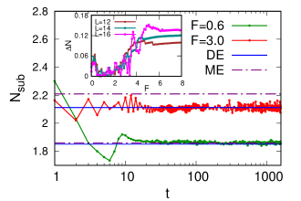
Figure 5: Quench dynamics: In the non-integrable ergodic phase ($F=0.6$), the long time saturation value of the average number of particles in the subsystem matches with those of the diagonal ensemble and the micro-canonical ensemble. In the non-integrable MBL phase ($F=3.0$) on the other hand, the saturation value matches with the result of the diagonal ensemble while it differs from that of the micro-canonical ensemble. The inset shows the normalized difference between the diagonal ensemble result and the micro-canonical ensemble result as a function of field strength for the same initial state. The value is close to zero in the non-integrable ergodic phase while a finite difference is obtained in the non-integrable MBL phase. The other parameters are: $L=16,\alpha=1.0,V=1.0$ filling factor $=0.5$, and subsystem size $m=4$.

Finally, we test the equivalence of thermodynamic entropy and entanglement entropy on varying the subsystem size. For each eigenstate, Fig. 4 shows the difference between these two for various values of subsystem size. It can be seen that for smaller subsystems the difference tends to zero, hence the smaller the subsystem the better is the thermalization Vidmar et al. (2017, 2018). The other two figures in Fig. 4 show the finite size scaling of this difference but for a single eigenstate located at the center of the spectrum. It can be seen that for a smaller fraction $m/L$ the difference goes to zero and thus shows the validity of ETH for these fractions. On the other hand, in the MBL phase, this difference is found to increase on increasing the system size as well as the subsystem sizes.

IV.2 Quench dynamics

A complementary understanding of the distinction between the various phases is afforded by a study of the long time behavior of the system under time evolution. As evident from Eq. 4, the dynamics of any observable has two parts: the first part is the same as the result predicted by the diagonal ensemble while the second part gives the fluctuations around it. In the long time limit, the observable, in general, equilibrates to the diagonal ensemble value. However this does not imply the thermalization of the observable. An observable is said to thermalize if the result of the diagonal ensemble matches with the result predicted by any thermal ensemble such as micro-canonical or canonical.

We consider the average number of particles in the subsystem (Li et al., 2015): $\hat{\mathcal{O}}=\sum_{i=1}^{m}\hat{N}_{i}$, where $\hat{N}_{i}=c_{i}^{\dagger}c_{i}$ is the number operator at site $i$. The initial state is taken as a charge density wave state (where all the even sites are occupied and odd sites are empty), and the dynamics is governed by the final Hamiltonian (Eq. II). The prescription for obtaining the micro-canonical density matrix is as follows. We first calculate the average energy of the initial state: $E_{\text{ini}}=\langle\psi_{0}|H|\psi_{0}\rangle$. Next we obtain the eigenstate closest to this energy. By taking $100$ nearest neighbor eigenstates around the obtained state, we then construct the micro-canonical density matrix.

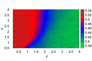
Figure 6: Surface plot of the level statistics as a function of both field strength $(F)$ and the interaction strength $(V)$. The other parameters are: $L=16,\alpha=1.0$.

We present data for the dynamics of the above observable in Fig. 5, comparing against the values predicted by the diagonal and micro-canonical ensembles. In the ergodic phase, the long time limit of the expectation value of the observable is in agreement with that predicted by both the diagonal ensemble and the micro-canonical ensemble, which in turn implies thermalization and the validity of ETH in this phase. On the other hand, in the MBL phase the saturation value is the same as predicted by the diagonal ensemble but it differs from the micro-canonical ensemble result suggesting the lack of thermalization in the MBL phase. To study the difference between the diagonal and micro-canonical ensemble results, we define the following normalized difference:

$$\Delta N=\frac{|N_{\text{DE}}-N_{\text{ME}}|}{|N_{\text{ME}}|},$$ (11)

where $N_{\text{DE}}$ and $N_{\text{ME}}$ are the expectation values of the observable $\hat{\mathcal{O}}$, calculated from the diagonal ensemble and micro-canonical ensemble respectively. The inset shows the normalized difference $\Delta N$ (Eq. 11) as a function of electric field strength for the same initial state. The value is close to zero in the non-integrable ergodic phase while a finite difference is obtained in the non-integrable MBL phase.

IV.3 Variation of interaction strength

The nature of the phase obtained also depends on the interaction strength. Fig. 6 shows the surface plot of the average level spacing as a function of both field strength and interaction strength for a fixed value of the curvature term ($\alpha=1.0$). It can be seen that on increasing the interaction strength, the ergodic region extends, thus we expect the equivalence of the entanglement entropy and the thermodynamic entropy to hold in this extended region.

V Summary and Conclusions

To summarize, we test the validity of ETH in an interacting system subjected to a static electric field. For small electric field strength this model shows ergodic behavior while for sufficiently strong electric field it exhibits MBL. In the limit of zero electric field and curvature strength, the model is integrable. We find that in the ergodic phase, the entanglement entropy of the states following a volume law of scaling matches with the corresponding thermodynamic entropy thus satisfying the ETH criterion, while in the MBL phase, the entanglement entropy fluctuates wildly from eigenstate to eigenstate, and also differs from the thermodynamic entropy. Since the MBL phase possesses low entanglement, a clear distinction is obtained between the integrable and the MBL phase from the point of view of the ETH. As reported earlier (Deutsch et al., 2013), a striking distinction between integrable and non-integrable systems is the presence of large eigenstate-to-eigenstate fluctuations in the expectation value of any observable in the integrable case. In support of the argument that the MBL phase is similar to integrable systems, we find that indeed, the MBL phase is also characterized by large flucutations in entanglement entropy across adjacent eigenstates. However, in contrast to the integrable phase, the magnitude of entanglement is significantly lower in the MBL phase. Moreover, the difference between the average entropy and the thermodynamic entropy increases on going deep into the localized phase.

We further verify the above arguments from a dynamical perspective by studying the dynamics of average number of particles in the subsystem starting from a charge density wave type of initial state. We find that in the ergodic phase the saturation value obtained from the dynamics, the result predicted by the diagonal ensemble as well as the micro-canonical ensemble result match with each other, implying that the system thermalizes in the long time limit. In the MBL phase on the other hand, the saturation value matches with the result predicted by the diagonal ensemble, but differs from that predicted by the micro-canonical ensemble. This signifies the lack of thermalization or ETH in the MBL phase.

Appendix A Scaling of Entanglement Entropy and Thermodynamic Entropy

In this appendix, we provide the scaling of the entanglement entropy and the thermodynamic entropy of two random states from the middle of the spectrum as a function of subsystem size. In the ergodic phase ($F=0.2$), both the entropy matches with each other and follows a volume law scaling, while in the MBL phase $(F=3.0)$, only the thermodynamic entropy shows a volume law scaling (Fig. 7).

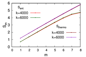
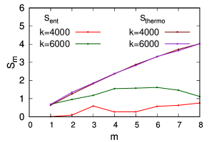
Figure 7: The scaling of entanglement entropy and thermodynamic entropy as a function of subsystem size for two different eigenvectors in the middle of the spectrum. In the ergodic phase ($F=0.2$), both follows a volume law scaling (Left). The thermodynamic entropy is shifted by an amount $0.5$ from the clarity purpose. In the MBL phase $(F=3.0)$, only the thermodynamic entropy shows a volume law scaling (right). The other parameters are: $L=16,\alpha=1.0\ \text{and}\ \ V=1.0$.

References

- Huang (2009) K. Huang, Introduction to statistical physics (Chapman and Hall/CRC, 2009).
- Pathria and Beale (2011) R. Pathria and P. Beale, Statistical Mechanics (Elsevier Science, 2011).
- Penrose (1979) O. Penrose, Reports on Progress in Physics 42, 1937 (1979).
- Kinoshita et al. (2006) T. Kinoshita, T. Wenger, and D. S. Weiss, Nature 440, 900 (2006).
- Hofferberth et al. (2007) S. Hofferberth, I. Lesanovsky, B. Fischer, T. Schumm, and J. Schmiedmayer, Nature 449, 324 (2007).
- Rigol et al. (2008) M. Rigol, V. Dunjko, and M. Olshanii, Nature 452, 854 (2008).
- Rigol (2009) M. Rigol, Phys. Rev. Lett. 103, 100403 (2009).
- Santos and Rigol (2010a) L. F. Santos and M. Rigol, Phys. Rev. E 82, 031130 (2010a).
- Rigol and Fitzpatrick (2011) M. Rigol and M. Fitzpatrick, Physical Review A 84, 033640 (2011).
- He and Rigol (2012) K. He and M. Rigol, Physical Review A 85, 063609 (2012).
- Mondaini and Rigol (2015) R. Mondaini and M. Rigol, Physical Review A 92, 041601 (2015).
- Beugeling et al. (2014a) W. Beugeling, R. Moessner, and M. Haque, Phys. Rev. E 89, 042112 (2014a).
- Rigol et al. (2007) M. Rigol, V. Dunjko, V. Yurovsky, and M. Olshanii, Physical review letters 98, 050405 (2007).
- Santos and Rigol (2010b) L. F. Santos and M. Rigol, Phys. Rev. E 81, 036206 (2010b).
- Canovi et al. (2011) E. Canovi, D. Rossini, R. Fazio, G. E. Santoro, and A. Silva, Physical Review B 83, 094431 (2011).
- Rigol and Santos (2010) M. Rigol and L. F. Santos, Physical Review A 82, 011604 (2010).
- Vitagliano et al. (2010) G. Vitagliano, A. Riera, and J. I. Latorre, New Journal of Physics 12, 113049 (2010).
- Wolf (2006) M. M. Wolf, Phys. Rev. Lett. 96, 010404 (2006).
- Lai et al. (2013) H.-H. Lai, K. Yang, and N. E. Bonesteel, Phys. Rev. Lett. 111, 210402 (2013).
- Roy and Sharma (2018) N. Roy and A. Sharma, Physical Review B 97, 125116 (2018).
- Roy et al. (2019) N. Roy, A. Sharma, and R. Mukherjee, Physical Review A 99, 052342 (2019).
- Pouranvari and Yang (2014) M. Pouranvari and K. Yang, Phys. Rev. B 89, 115104 (2014).
- Hastings (2007) M. B. Hastings, Journal of Statistical Mechanics: Theory and Experiment 2007, P08024 (2007).
- Laflorencie (2016) N. Laflorencie, Physics Reports 646, 1 (2016).
- Eisert et al. (2010) J. Eisert, M. Cramer, and M. B. Plenio, Reviews of Modern Physics 82, 277 (2010).
- Deutsch et al. (2013) J. Deutsch, H. Li, and A. Sharma, Physical Review E 87, 042135 (2013).
- Deutsch (1991) J. M. Deutsch, Phys. Rev. A 43, 2046 (1991).
- Srednicki (1994) M. Srednicki, Phys. Rev. E 50, 888 (1994).
- Deutsch (2018) J. M. Deutsch, Reports on Progress in Physics 81, 082001 (2018).
- D’Alessio et al. (2016) L. D’Alessio, Y. Kafri, A. Polkovnikov, and M. Rigol, Advances in Physics 65, 239 (2016).
- Deutsch (2010) J. Deutsch, New Journal of Physics 12, 075021 (2010).
- Gornyi et al. (2005) I. V. Gornyi, A. D. Mirlin, and D. G. Polyakov, Phys. Rev. Lett. 95, 206603 (2005).
- Basko et al. (2006) D. M. Basko, I. L. Aleiner, and B. L. Altshuler, Annals of physics 321, 1126 (2006).
- Anderson (1958) P. W. Anderson, Phys. Rev. 109, 1492 (1958).
- Nandkishore and Huse (2015) R. Nandkishore and D. A. Huse, Annu. Rev. Condens. Matter Phys. 6, 15 (2015).
- Pal and Huse (2010) A. Pal and D. A. Huse, Physical review b 82, 174411 (2010).
- Vosk and Altman (2013) R. Vosk and E. Altman, Physical review letters 110, 067204 (2013).
- Huse et al. (2014) D. A. Huse, R. Nandkishore, and V. Oganesyan, Physical Review B 90, 174202 (2014).
- Vasseur and Moore (2016) R. Vasseur and J. E. Moore, Journal of Statistical Mechanics: Theory and Experiment 2016, 064010 (2016).
- Abanin et al. (2019) D. A. Abanin, E. Altman, I. Bloch, and M. Serbyn, Rev. Mod. Phys. 91, 021001 (2019).
- Imbrie et al. (2017) J. Z. Imbrie, V. Ros, and A. Scardicchio, Annalen der Physik 529, 1600278 (2017).
- Serbyn et al. (2013) M. Serbyn, Z. Papić, and D. A. Abanin, Physical review letters 111, 127201 (2013).
- Chandran et al. (2015) A. Chandran, I. H. Kim, G. Vidal, and D. A. Abanin, Physical Review B 91, 085425 (2015).
- Khatami et al. (2012a) E. Khatami, M. Rigol, A. Relano, and A. M. García-García, Physical Review E 85, 050102 (2012a).
- He et al. (2013) K. He, L. F. Santos, T. M. Wright, and M. Rigol, Physical Review A 87, 063637 (2013).
- Tang et al. (2015) B. Tang, D. Iyer, and M. Rigol, Physical Review B 91, 161109 (2015).
- Beugeling et al. (2014b) W. Beugeling, R. Moessner, and M. Haque, Physical Review E 89, 042112 (2014b).
- Kim et al. (2014) H. Kim, T. N. Ikeda, and D. A. Huse, Physical Review E 90, 052105 (2014).
- Rigol and Srednicki (2012) M. Rigol and M. Srednicki, Phys. Rev. Lett. 108, 110601 (2012).
- Ikeda et al. (2013) T. N. Ikeda, Y. Watanabe, and M. Ueda, Phys. Rev. E 87, 012125 (2013).
- Khatami et al. (2012b) E. Khatami, M. Rigol, A. Relaño, and A. M. García-García, Phys. Rev. E 85, 050102 (2012b).
- Sutherland (2004) B. Sutherland, Beautiful models: 70 years of exactly solved quantum many-body problems (World Scientific Publishing Company, 2004).
- Luitz et al. (2015) D. J. Luitz, N. Laflorencie, and F. Alet, Physical Review B 91, 081103 (2015).
- Iyer et al. (2013) S. Iyer, V. Oganesyan, G. Refael, and D. A. Huse, Physical Review B 87, 134202 (2013).
- Schulz et al. (2019) M. Schulz, C. Hooley, R. Moessner, and F. Pollmann, Physical review letters 122, 040606 (2019).
- van Nieuwenburg et al. (2019) E. van Nieuwenburg, Y. Baum, and G. Refael, Proceedings of the National Academy of Sciences 116, 9269 (2019).
- Moudgalya et al. (2019) S. Moudgalya, A. Prem, R. Nandkishore, N. Regnault, and B. A. Bernevig, arXiv preprint arXiv:1910.14048 (2019).
- Taylor et al. (2019) S. R. Taylor, M. Schulz, F. Pollmann, and R. Moessner, arXiv preprint arXiv:1910.01154 (2019).
- Schreiber et al. (2015) M. Schreiber, S. S. Hodgman, P. Bordia, H. P. Lüschen, M. H. Fischer, R. Vosk, E. Altman, U. Schneider, and I. Bloch, Science 349, 842 (2015).
- Choi et al. (2016) J.-y. Choi, S. Hild, J. Zeiher, P. Schauß, A. Rubio-Abadal, T. Yefsah, V. Khemani, D. A. Huse, I. Bloch, and C. Gross, Science 352, 1547 (2016).
- Smith et al. (2016) J. Smith, A. Lee, P. Richerme, B. Neyenhuis, P. W. Hess, P. Hauke, M. Heyl, D. A. Huse, and C. Monroe, Nature Physics 12, 907 (2016).
- Kondov et al. (2015) S. Kondov, W. McGehee, W. Xu, and B. DeMarco, Physical review letters 114, 083002 (2015).
- Bordia et al. (2017) P. Bordia, H. Lüschen, S. Scherg, S. Gopalakrishnan, M. Knap, U. Schneider, and I. Bloch, Physical Review X 7, 041047 (2017).
- Krieger and Iafrate (1986) J. Krieger and G. Iafrate, Physical Review B 33, 5494 (1986).
- Wannier (1960) G. H. Wannier, Physical Review 117, 432 (1960).
- Bouchard and Luban (1995) A. Bouchard and M. Luban, Physical Review B 52, 5105 (1995).
- Mendez and Bastard (1993) E. E. Mendez and G. Bastard, Physics Today 46, 34 (1993).
- Hartmann et al. (2004) T. Hartmann, F. Keck, H. Korsch, and S. Mossmann, New Journal of Physics 6, 2 (2004).
- Bhakuni and Sharma (2018) D. S. Bhakuni and A. Sharma, Phys. Rev. B 98, 045408 (2018).
- Bhakuni et al. (2019) D. S. Bhakuni, S. Dattagupta, and A. Sharma, Phys. Rev. B 99, 155149 (2019).
- Oganesyan and Huse (2007) V. Oganesyan and D. A. Huse, Physical review b 75, 155111 (2007).
- Atas et al. (2013) Y. Atas, E. Bogomolny, O. Giraud, and G. Roux, Physical review letters 110, 084101 (2013).
- Xu et al. (2019) S. Xu, X. Li, Y.-T. Hsu, B. Swingle, and S. D. Sarma, arXiv preprint arXiv:1902.07199 (2019).
- Vidmar et al. (2017) L. Vidmar, L. Hackl, E. Bianchi, and M. Rigol, Phys. Rev. Lett. 119, 020601 (2017).
- Vidmar et al. (2018) L. Vidmar, L. Hackl, E. Bianchi, and M. Rigol, Phys. Rev. Lett. 121, 220602 (2018).
- Li et al. (2015) X. Li, S. Ganeshan, J. H. Pixley, and S. Das Sarma, Phys. Rev. Lett. 115, 186601 (2015).