Weak-lensing Analysis of X-Ray-selected XXL Galaxy Groups and Clusters with Subaru HSC Data

Abstract

We present a weak-lensing analysis of X-ray galaxy groups and clusters selected from the XMM-XXL survey using the first-year data from the Hyper Suprime-Cam (HSC) Subaru Strategic Program. Our joint weak-lensing and X-ray analysis focuses on 136 spectroscopically confirmed X-ray-selected systems at $0.031\leqslant z\leqslant 1.033$ detected in the 25 deg² XXL-N region, which largely overlaps with the HSC-XMM field. With high-quality HSC weak-lensing data, we characterize the mass distributions of individual clusters and establish the concentration–mass ($c$–$M$) relation for the XXL sample, by accounting for selection bias and statistical effects and marginalizing over the remaining mass calibration uncertainty. We find the mass-trend parameter of the $c$–$M$ relation to be $\beta=-0.07\pm 0.28$ and the normalization to be $c_{200}=4.8\pm 1.0\,(\mathrm{stat})\pm 0.8\,(\mathrm{syst})$ at $M_{200}=10^{14}h^{-1}M_{\odot}$ and $z=0.3$. We find no statistical evidence for redshift evolution. Our weak-lensing results are in excellent agreement with dark-matter-only $c$–$M$ relations calibrated for recent $\Lambda$CDM cosmologies. The level of intrinsic scatter in $c_{200}$ is constrained as $\sigma(\ln{c_{200}})<24\%$ ($99.7\%$ CL), which is smaller than predicted for the full population of $\Lambda$CDM halos. This is likely caused in part by the X-ray selection bias in terms of the cool-core or relaxation state. We determine the temperature–mass ($T_{\mathrm{X}}$–$M_{500}$) relation for a subset of 105 XXL clusters that have both measured HSC lensing masses and X-ray temperatures. The resulting $T_{\mathrm{X}}$–$M_{500}$ relation is consistent with the self-similar prediction. Our $T_{\mathrm{X}}$–$M_{500}$ relation agrees with the XXL DR1 results at group scales but has a slightly steeper mass trend, implying a smaller mass scale in the cluster regime. The overall offset in the $T_{\mathrm{X}}$–$M_{500}$ relation is at the $\sim 1.5\sigma$ level, corresponding to a mean mass offset of $(34\pm 20)\%$. We also provide bias-corrected, weak-lensing-calibrated $M_{200}$ and $M_{500}$ mass estimates of individual XXL clusters based on their measured X-ray temperatures.

1. Introduction

Galaxy clusters represent the largest bound objects formed in the universe. Since galaxy clusters are highly massive and dominated by dark matter (DM), they offer fundamental tests on the assumed properties of DM. For example, the standard cold dark matter (CDM) paradigm assumes that DM is effectively cold and collisionless on astrophysical scales (Bertone & Tait, 2018). In this context, the standard CDM model and its variants can provide a series of observationally testable predictions. A prime example is the “Bullet Cluster”, a merging pair of galaxy clusters exhibiting a significant offset between the centers of the gravitational lensing mass and the peaks of the collisional intracluster gas (Clowe et al., 2004, 2006). The data support that DM is effectively collisionless, like galaxies, placing a robust upper limit on the self-interacting DM cross section of $\sigma_{\mathrm{DM}}/m<1.25$ cm² g^-1 (Randall et al., 2008).

The evolution of the abundance of clusters across cosmic time is sensitive to the amplitude and growth rate of primordial density fluctuations, as well as to the cosmic volume–redshift relation. This cosmological sensitivity mainly comes from the fact that cluster halos populate the exponential tail of the cosmic mass function (Haiman et al., 2001; Watson et al., 2014). Hence, large samples of galaxy clusters spanning a wide range of masses and redshifts provide an independent means of examining any viable cosmological model (Allen et al., 2004; Vikhlinin et al., 2009b; Mantz et al., 2010; Pratt et al., 2019). In principle, galaxy clusters can thus complement other cosmological probes, such as cosmic microwave background (CMB) anisotropy, large-scale galaxy clustering, distant supernovae, and cosmic shear observations.

Significant progress has been made in recent years in constructing large statistical samples of clusters thanks to dedicated wide-field surveys (e.g., Planck Collaboration et al., 2014, 2016; Bleem et al., 2015; Rykoff et al., 2016; Oguri et al., 2018; Miyazaki et al., 2018a). Cluster samples are often defined by X-ray, Sunyaev–Zel’dovich effect (SZE), or optical imaging observables, so that the cluster masses are statistically inferred from mass scaling relations. Since the level of mass bias is likely cluster mass dependent (Sereno et al., 2015a; Sereno & Ettori, 2017) and sensitive to calibration systematics of the instruments (Donahue et al., 2014; Israel et al., 2015), a concerted effort is required to enable an accurate calibration of mass scaling relations using direct weak-lensing mass measurements (e.g., von der Linden et al., 2014; Applegate et al., 2014; Umetsu et al., 2014; Hoekstra et al., 2015; Melchior et al., 2015; Okabe & Smith, 2016; Sereno et al., 2017; Schrabback et al., 2018) and well-defined selection functions (e.g., Benitez et al., 2014).

The distribution and concentration of DM in quasi-equilibrium objects depend fundamentally on the properties of DM. Hierarchical CDM models predict that the structure of halos characterized in terms of the spherically averaged density profile $\rho(r)$ is approximately self-similar with a characteristic density cusp in their centers, $\rho(r)\propto 1/r$, albeit with large variance associated with the assembly histories of individual halos (Jing & Suto, 2000). They also predict that the density gradient $d\ln{\rho(r)/d\ln{r}}$ of DM halos continuously steepens from the center out to diffuse outskirts (Navarro et al., 1996, 1997, hereafter NFW). Clusters are predicted to have lower central concentrations, in contrast to individual galaxies that have denser central regions (Diemer & Kravtsov, 2015). The shape of clusters is predicted to be not spherical but triaxial, reflecting the collisionless nature of DM (Jing & Suto, 2002).

Gravitational lensing offers a direct probe of the cosmic matter distribution dominated by DM. While strong lensing leads to highly distorted and/or multiple images in the densest regions of the universe (e.g., Hattori et al., 1999), namely the central regions of massive halos, weak lensing provides a direct measure of the mass distribution on larger scales (e.g., Bartelmann & Schneider, 2001). Galaxy clusters act as powerful gravitational lenses, producing both strong- and weak-lensing features in the images of background source galaxies. The unique advantage of weak gravitational lensing is its ability to constrain the mass distribution of individual systems independently of assumptions about their physical or dynamical state.

Weak-lensing observations in the cluster regime have established that the total matter distribution within clusters in projection can be well described by cuspy, outward steepening density profiles (Umetsu et al., 2011b, 2014, 2016; Newman et al., 2013; Okabe et al., 2013), with a near-universal shape (Niikura et al., 2015; Umetsu & Diemer, 2017), as predicted for collisionless halos in quasi-gravitational equilibrium (e.g., Navarro et al., 1996, 1997; Taylor & Navarro, 2001; Hjorth & Williams, 2010; Williams & Hjorth, 2010). Subsequent cluster lensing studies targeting lensing-unbiased samples (e.g., Merten et al., 2015; Du et al., 2015; Umetsu et al., 2016; Okabe & Smith, 2016; Cibirka et al., 2017; Sereno et al., 2017; Klein et al., 2019) have found that the degree of mass concentration derived for these clusters agrees well with theoretical models calibrated for recent $\Lambda$CDM cosmologies (e.g., Bhattacharya et al., 2013; Dutton & Macciò, 2014; Meneghetti et al., 2014; Diemer & Kravtsov, 2015). The three-dimensional shapes of galaxy clusters as constrained by weak-lensing and multiwavelength data sets are found to be in agreement with $\Lambda$CDM predictions (e.g., Oguri et al., 2005; Morandi et al., 2012; Sereno et al., 2013, 2018; Umetsu et al., 2015). These results are all in support of the standard explanation for DM as effectively collisionless and nonrelativistic on sub-Mpc scales and beyond, with an excellent match with standard $\Lambda$CDM predictions.

The XXL program (Pierre et al., 2016, hereafter XXL Paper I) represents one of the largest XMM-Newton programs to date. The ultimate science goal of the XXL survey is to provide independent and self-sufficient cosmological constraints using X-ray-selected galaxy clusters (Pacaud et al., 2016, hereafter XXL Paper II). The XXL survey covers two sky regions of $\simeq 25$ deg² each at high galactic latitudes, namely, the XXL-N and XXL-S fields. With the aid of multiwavelength follow-up observations, the survey has uncovered nearly 400 galaxy groups and clusters out to a redshift of $z\sim 2$ (Adami et al., 2018, hereafter XXL Paper XX), spanning approximately two decades in mass (XXL Paper I). This XXL 365 galaxy cluster catalog was made public as part of the XXL second-year data release (DR2).

Hyper Suprime-Cam is an optical wide-field imager with a 1.77 deg² field of view mounted on the prime focus of the 8.2 m Subaru telescope (Miyazaki et al., 2018b; Komiyama et al., 2018; Furusawa et al., 2018; Kawanomoto et al., 2018). The Hyper Suprime-Cam Subaru Strategic Program (HSC-SSP; Aihara et al., 2018b, a) has been conducting an optical imaging survey in five broad bands ($grizy$) in three layers of survey depths and areas (Wide, Deep, and Ultradeep), aiming at observing $1400$ deg² on the sky in its Wide layer (Aihara et al., 2018b). The HSC survey is optimized for weak-lensing studies (Mandelbaum et al., 2018a; Miyaoka et al., 2018; Medezinski et al., 2018b; Hikage et al., 2019; Hamana et al., 2020) and overlaps with the XXL survey in its HSC-XMM field. It is therefore possible to directly estimate the masses of XXL clusters using well-calibrated weak-lensing data available from the HSC survey.

In this paper, we carry out a weak-lensing analysis on a statistical sample of X-ray groups and clusters drawn from the XXL DR2 cluster catalog (XXL Paper XX). Our analysis uses wide-field multiband imaging from the HSC survey to measure the weak-lensing signal for our XXL sample. The main goal of this paper is to obtain cluster mass estimates for individual XXL clusters and to achieve ensemble mass calibration with sufficient accuracy for scaling relation analyses. With direct mass measurements from weak lensing, we aim to characterize observable–mass scaling relations of the XXL sample. We focus on the concentration–mass ($c$–$M$) and temperature–mass ($T_{\mathrm{X}}$–$M$) relations in this work. In our companion paper (Sereno et al., 2020), we examine joint multivariate X-ray observable–mass scaling relations for the XXL sample using the cluster mass measurements presented in this paper.

This paper is organized as follows. Section 2 describes the XXL cluster catalog and the HSC-SSP data. Section 3 describes the weak-lensing measurements, the selection of background galaxies, and their associated uncertainties (see also Appendix A). In Section 4, after describing the methodology used to infer the mass and concentration parameters from the lensing signal, we present the results of weak-lensing mass measurements of the XXL sample. In Section 5 we examine observable–mass scaling relations of the XXL sample through Bayesian population modeling. Finally, a summary is given in Section 6.

Throughout this paper, we assume a spatially flat $\Lambda$CDM cosmology with $\Omega_{\mathrm{m}}=0.28$, $\Omega_{\Lambda}=0.72$, and a Hubble constant of $H_{0}=100h$ km s^-1 Mpc^-1 with $h=0.7$. We adopt $\sigma_{8}=0.817$ (Hinshaw et al., 2013) for the fiducial normalization of the matter power spectrum, with $\sigma_{8}$ the rms amplitude of linear mass fluctuations in a sphere of comoving radius $8h^{-1}\mathrm{Mpc}$. We denote the critical density of the universe at a particular redshift $z$ as $\rho_{\mathrm{c}}(z)=3H^{2}(z)/(8\pi G)$, with $H(z)$ the redshift-dependent Hubble parameter. We also define the dimensionless expansion function as $E(z)=H(z)/H_{0}$. We adopt the standard notation $M_{\Delta}$ to denote the mass enclosed within a sphere of radius $r_{\Delta}$ within which the mean overdensity equals $\Delta\times\rho_{\mathrm{c}}(z)$. We denote three-dimensional cluster radii as $r$, and reserve the symbol $R$ for projected cluster-centric distances.

We use “$\log$” to denote the base-10 logarithm and “$\ln$” to denote the natural logarithm. The fractional scatter in natural logarithm is quoted as a percent. All quoted errors are $1\sigma$ confidence limits unless otherwise stated.

2. Cluster Sample and Data

2.1. XXL Cluster Sample

Table 1 Characteristics of the XXL samples

Sample	$N_{\mathrm{cl}}$	$N_{T}$	$T_{\mathrm{X}}$	$\langle T_{\mathrm{X}}\rangle_{\mathrm{wl}}$	$z$	$\langle z\rangle_{\mathrm{wl}}$	$c_{200}$	$M_{200}$	$\langle M_{200}\rangle_{\mathrm{wl}}$	$\langle M_{200}\rangle_{\mathrm{g}}$	SNR	$($SNR$)_{\mathrm{q}}$
			(keV)	(keV)				($10^{13}h^{-1}M_{\odot}$)	($10^{13}h^{-1}M_{\odot}$)	($10^{13}h^{-1}M_{\odot}$)
C1+C2	$136$	$105$	$1.9$	$2.0$	$0.30$	$0.25$	$3.5\pm 0.9$	$8.7\pm 0.8$	$8.0\pm 0.8$	$9.8\pm 0.8$	$15.6$	$20.5$
C1	$83$	$76$	$2.1$	$2.1$	$0.29$	$0.23$	$3.6\pm 1.1$	$9.7\pm 1.0$	$9.0\pm 1.0$	$11.6\pm 1.2$	$14.0$	$18.4$
C2	$53$	$29$	$1.7$	$1.6$	$0.43$	$0.29$	$3.4\pm 1.8$	$6.4\pm 1.2$	$6.1\pm 1.1$	$6.5\pm 1.0$	$7.2$	$9.5$

Note. — Quantities in brackets with subscript ”wl” denote lensing-weighted sample means (Equation (27)), and those in brackets with subscript ”g”e denote error-weighted geometric means (Equation (24)). The effective mass and concentration parameters ($M_{200},c_{200}$) of each subsample are obtained from a single-mass-bin fit to the respective stacked $\Delta\Sigma$ profile assuming an NFW density profile. For each sample, the effective $M_{200}$ mass is consistent with the respective weighted sample averages from individual cluster weak-lensing measurements. We provide two different estimates of the weak-lensing signal-to-nose ratio integrated over the comoving radial range $R\in[0.3,3]\,h^{-1}\mathrm{Mpc}$, one based on the linear estimator, SNR (Equation (13)), and the other based on the quadratic estimator, $($SNR$)_{\mathrm{q}}$ (Equation (15)).

Figure 1.— Distribution of spectroscopically confirmed XXL-N C1+C2 groups and clusters (filled circles) in the HSC-XMM field. There are a total of 136 XXL systems selected for our HSC weak-lensing analysis. The circles marked with red edges represent C2 clusters. The gray shaded area shows the HSC survey footprint. The blue line shows the boundary of the combined exposure map of all XMM pointings in the XXL-N field. The area of the overlap region between the two surveys is $21.4$ deg². The cluster redshift is color-coded according to the color bar on the right side.

Figure 2.— Distribution of our cluster sample in the X-ray flux ($f_{60}$) versus redshift ($z$) plane. The gray circles and red crosses represent the C1 and C2 subsamples, respectively.

In the present study, we focus on spectroscopically confirmed X-ray-selected systems of class C1 and C2 drawn from the XXL DR2 catalog presented in XXL Paper XX. The C1 population is designed to be free of contamination by spurious detections or blended point sources, while the C2 population is deeper but its initial selection is about $50\%$ contaminated (XXL Paper I). Both populations of XXL clusters have been cleaned up a posteriori by optical spectroscopic observations and from a detailed comparison of X-ray and optical observations.

For our joint HSC-XXL analysis, we select XXL clusters that overlap with the HSC survey footprint within a comoving transverse separation of $R_{\mathrm{min}}=0.3h^{-1}\mathrm{Mpc}$, which is the minimum cluster-centric radius adopted in our HSC weak-lensing studies (Section 3.2; see also Medezinski et al., 2018b, a; Miyatake et al., 2019). These selection criteria leave us with 83 C1 clusters ($0.044\leqslant z\leqslant 1.002$) and 53 C2 clusters ($0.031\leqslant z\leqslant 1.033$), a total of 136 XXL clusters with spectroscopic confirmation. Of these, a subset of 105 clusters (76 C1 and 29 C2 clusters) have X-ray temperatures $T_{\mathrm{X}}=T_{\mathrm{300\,kpc}}$ measured in a fixed, core-included aperture of $300$ kpc, spanning the range $0.6\leqslant T_{\mathrm{300\,kpc}}/(\mathrm{keV})\leqslant 6.0$. Here the X-ray temperatures $T_{\mathrm{300\,kpc}}$ were measured with a spectral analysis of the cluster single best pointing (XXL Paper XX). Spectra were extracted for each of the XMM-Newton cameras from the region within a $300$ kpc aperture and fitted in the 0.4–11.0 keV band with the absorbed Astrophysical Plasma Emission Code model (v2.0.2) in XSPEC (Dorman et al., 2003), with a fixed metal abundance of $Z=0.3Z_{\odot}$. The background was modeled following Eckert et al. (2014). X-ray temperatures could not be measured for all clusters, because several cluster observations were at very low redshift with poor spatial coverage, were affected by flaring, were contaminated by point sources, or had very low X-ray counts.

Table 2 Cluster Properties and Weak-lensing Measurements

ID	R.A.	Decl.	$z$	Class	$T_{\mathrm{300\,kpc}}$	$c_{200}$	$M_{\mathrm{200}}$	$M_{\mathrm{500}}$	$M_{\mathrm{200,MT}}$	$M_{\mathrm{500,MT}}$	SNR	$($SNR$)_{\mathrm{q}}$
	(deg)	(deg)			(keV)		($10^{14}M_{\odot}$)	($10^{14}M_{\odot}$)	($10^{14}M_{\odot}$)	($10^{14}M_{\odot}$)
002	$36.384$	$-3.920$	$0.771$	1	$2.50^{+0.18}_{-0.19}$	$5.1\pm 4.9$ ($4.0$)	$0.19\pm 0.36$ ($0.36$)	$0.13\pm 0.25$ ($0.24$)	$1.07^{+0.90}_{-0.53}$	$0.72^{+0.65}_{-0.36}$	$0.3$	$1.7$
003	$36.909$	$-3.300$	$0.836$	1	$3.48^{+0.24}_{-0.25}$	$4.9\pm 4.8$ ($4.0$)	$0.43\pm 0.92$ ($0.87$)	$0.29\pm 0.62$ ($0.59$)	$1.64^{+1.39}_{-0.81}$	$1.11^{+1.02}_{-0.56}$	$0.7$	$2.5$
006	$35.439$	$-3.772$	$0.429$	1	$4.24^{+0.61}_{-0.45}$	$2.1\pm 1.2$ ($2.0$)	$9.64\pm 4.38$ ($9.45$)	$5.59\pm 2.09$ ($5.53$)	$6.79^{+3.38}_{-2.20}$	$4.72^{+1.92}_{-1.35}$	$5.7$	$6.6$
008	$36.336$	$-3.801$	$0.299$	1	$1.56^{+0.12}_{-0.10}$	$2.4\pm 2.0$ ($2.4$)	$1.65\pm 1.67$ ($1.46$)	$1.01\pm 0.95$ ($0.91$)	$1.07^{+0.81}_{-0.46}$	$0.74^{+0.56}_{-0.32}$	$3.2$	$3.5$
009	$36.685$	$-3.684$	$0.328$	2	–	$5.8\pm 5.1$ ($4.7$)	$0.42\pm 0.53$ ($0.33$)	$0.29\pm 0.37$ ($0.23$)	–	–	$1.0$	$3.3$
010	$36.843$	$-3.362$	$0.330$	1	$2.36^{+0.35}_{-0.24}$	$4.2\pm 4.2$ ($3.7$)	$1.13\pm 1.14$ ($1.01$)	$0.76\pm 0.74$ ($0.68$)	$1.36^{+0.99}_{-0.59}$	$0.92^{+0.70}_{-0.41}$	$2.1$	$4.1$
011	$36.540$	$-4.969$	$0.054$	1	$1.57^{+0.29}_{-0.11}$	$3.0\pm 3.0$ ($2.9$)	$1.15\pm 1.38$ ($1.00$)	$0.76\pm 0.84$ ($0.65$)	$0.90^{+0.72}_{-0.41}$	$0.63^{+0.51}_{-0.29}$	$5.0$	$5.5$
013	$36.858$	$-4.538$	$0.308$	1	$1.30^{+0.22}_{-0.11}$	$2.8\pm 2.7$ ($2.7$)	$1.51\pm 1.43$ ($1.40$)	$0.97\pm 0.83$ ($0.90$)	$0.95^{+0.71}_{-0.40}$	$0.67^{+0.50}_{-0.28}$	$3.4$	$3.8$
018	$36.008$	$-5.091$	$0.324$	1	$1.68^{+0.24}_{-0.16}$	$5.9\pm 5.1$ ($4.7$)	$0.29\pm 0.40$ ($0.24$)	$0.20\pm 0.27$ ($0.17$)	$0.77^{+0.63}_{-0.37}$	$0.52^{+0.46}_{-0.26}$	$-0.4$	$2.8$
020	$36.635$	$-5.001$	$0.494$	2	$1.65^{+0.30}_{-0.23}$	$2.1\pm 1.6$ ($2.2$)	$4.36\pm 3.39$ ($4.14$)	$2.60\pm 1.80$ ($2.52$)	$1.89^{+1.39}_{-0.76}$	$1.39^{+0.95}_{-0.55}$	$3.6$	$3.9$
021	$36.233$	$-5.134$	$0.085$	1	$0.79^{+0.06}_{-0.06}$	$5.1\pm 4.8$ ($4.0$)	$0.10\pm 0.13$ ($0.10$)	$0.07\pm 0.09$ ($0.07$)	$0.29^{+0.23}_{-0.14}$	$0.19^{+0.17}_{-0.09}$	$3.2$	$4.5$
022	$36.917$	$-4.858$	$0.293$	1	$1.98^{+0.13}_{-0.12}$	$4.9\pm 4.5$ ($4.2$)	$2.15\pm 1.34$ ($2.11$)	$1.48\pm 0.87$ ($1.46$)	$1.67^{+0.98}_{-0.60}$	$1.20^{+0.69}_{-0.43}$	$2.6$	$3.9$
025	$36.353$	$-4.680$	$0.265$	1	$2.23^{+0.24}_{-0.18}$	$4.6\pm 4.5$ ($3.9$)	$0.96\pm 0.93$ ($0.86$)	$0.65\pm 0.61$ ($0.58$)	$1.24^{+0.88}_{-0.54}$	$0.84^{+0.62}_{-0.37}$	$1.6$	$3.5$
027	$37.012$	$-4.851$	$0.295$	1	$2.72^{+0.41}_{-0.40}$	$2.8\pm 2.7$ ($2.7$)	$0.91\pm 1.04$ ($0.77$)	$0.58\pm 0.63$ ($0.49$)	$1.45^{+1.13}_{-0.67}$	$0.95^{+0.77}_{-0.44}$	$2.6$	$3.5$
028	$35.984$	$-3.098$	$0.297$	1	$1.53^{+0.27}_{-0.17}$	$5.2\pm 4.9$ ($4.1$)	$0.24\pm 0.35$ ($0.21$)	$0.16\pm 0.24$ ($0.14$)	$0.71^{+0.59}_{-0.34}$	$0.48^{+0.43}_{-0.24}$	$0.2$	$2.6$
030	$35.778$	$-4.216$	$0.631$	2	–	$5.5\pm 5.0$ ($4.3$)	$0.09\pm 0.12$ ($0.10$)	$0.06\pm 0.08$ ($0.07$)	–	–	$-1.2$	$2.3$
032	$36.002$	$-3.424$	$0.803$	2	$2.16^{+0.49}_{-0.42}$	$5.2\pm 4.9$ ($4.1$)	$0.24\pm 0.47$ ($0.48$)	$0.16\pm 0.32$ ($0.32$)	$1.01^{+0.93}_{-0.51}$	$0.69^{+0.67}_{-0.35}$	$0.3$	$1.5$
035	$35.949$	$-2.858$	$0.174$	1	$1.26^{+0.08}_{-0.08}$	$5.5\pm 5.0$ ($4.3$)	$0.11\pm 0.14$ ($0.10$)	$0.07\pm 0.10$ ($0.07$)	$0.47^{+0.38}_{-0.23}$	$0.32^{+0.27}_{-0.15}$	$-0.0$	$3.4$
036	$35.527$	$-3.054$	$0.492$	1	$3.53^{+0.53}_{-0.43}$	$6.4\pm 5.3$ ($5.3$)	$0.52\pm 0.70$ ($0.41$)	$0.36\pm 0.50$ ($0.28$)	$1.63^{+1.33}_{-0.79}$	$1.10^{+0.98}_{-0.54}$	$0.5$	$3.9$
038	$36.856$	$-4.190$	$0.584$	2	$1.67^{+0.30}_{-0.28}$	$5.5\pm 5.0$ ($4.3$)	$0.09\pm 0.12$ ($0.09$)	$0.06\pm 0.08$ ($0.06$)	$0.60^{+0.52}_{-0.30}$	$0.39^{+0.36}_{-0.20}$	$-0.3$	$2.0$
040	$35.523$	$-4.547$	$0.320$	1	$1.95^{+0.26}_{-0.24}$	$5.4\pm 5.1$ ($4.2$)	$0.78\pm 0.85$ ($0.66$)	$0.54\pm 0.58$ ($0.45$)	$1.06^{+0.80}_{-0.47}$	$0.72^{+0.57}_{-0.33}$	$2.1$	$3.9$
041	$36.378$	$-4.239$	$0.142$	1	$1.68^{+0.22}_{-0.08}$	$7.3\pm 5.1$ ($6.5$)	$2.47\pm 1.11$ ($2.45$)	$1.82\pm 0.76$ ($1.82$)	$1.94^{+0.92}_{-0.60}$	$1.49^{+0.66}_{-0.45}$	$2.9$	$5.9$
044	$36.141$	$-4.236$	$0.263$	1	$1.21^{+0.11}_{-0.14}$	$2.9\pm 2.6$ ($2.8$)	$2.07\pm 1.40$ ($2.00$)	$1.32\pm 0.81$ ($1.30$)	$1.20^{+0.79}_{-0.45}$	$0.87^{+0.54}_{-0.32}$	$3.6$	$4.8$
048	$35.722$	$-3.473$	$1.005$	2	$2.72^{+0.18}_{-0.16}$	$5.7\pm 5.1$ ($4.6$)	$1.04\pm 2.61$ ($2.52$)	$0.71\pm 1.78$ ($1.71$)	$1.28^{+1.12}_{-0.63}$	$0.88^{+0.83}_{-0.44}$	$1.1$	$1.1$
049	$35.988$	$-4.588$	$0.494$	1	$2.13^{+0.12}_{-0.14}$	$6.0\pm 5.1$ ($4.9$)	$1.90\pm 1.84$ ($1.73$)	$1.35\pm 1.29$ ($1.21$)	$1.42^{+1.03}_{-0.60}$	$1.00^{+0.76}_{-0.43}$	$1.3$	$3.2$
050	$36.421$	$-3.189$	$0.140$	1	$3.07^{+0.26}_{-0.25}$	$6.3\pm 5.3$ ($5.1$)	$1.10\pm 0.96$ ($1.04$)	$0.78\pm 0.68$ ($0.72$)	$1.65^{+1.14}_{-0.71}$	$1.13^{+0.82}_{-0.49}$	$1.0$	$3.9$
051	$36.498$	$-2.825$	$0.279$	1	$1.34^{+0.09}_{-0.09}$	$6.1\pm 5.2$ ($4.9$)	$0.22\pm 0.32$ ($0.19$)	$0.15\pm 0.22$ ($0.13$)	$0.60^{+0.49}_{-0.29}$	$0.40^{+0.35}_{-0.20}$	$-0.3$	$3.2$
052	$36.567$	$-2.666$	$0.056$	1	$0.63^{+0.04}_{-0.03}$	$5.1\pm 4.9$ ($4.0$)	$0.12\pm 0.17$ ($0.12$)	$0.08\pm 0.11$ ($0.08$)	$0.23^{+0.19}_{-0.11}$	$0.16^{+0.14}_{-0.08}$	$0.8$	$2.5$
054	$36.319$	$-5.887$	$0.054$	1	$1.54^{+0.09}_{-0.08}$	$5.9\pm 5.2$ ($4.7$)	$0.60\pm 0.76$ ($0.48$)	$0.42\pm 0.54$ ($0.33$)	$0.77^{+0.60}_{-0.35}$	$0.53^{+0.44}_{-0.25}$	$-0.3$	$3.6$
055	$36.454$	$-5.896$	$0.232$	1	$3.15^{+0.32}_{-0.51}$	$8.2\pm 5.4$ ($7.5$)	$3.19\pm 1.49$ ($3.20$)	$2.39\pm 1.07$ ($2.39$)	$2.92^{+1.37}_{-0.92}$	$2.19^{+1.01}_{-0.69}$	$3.1$	$4.8$
056	$33.871$	$-4.682$	$0.348$	1	$2.99^{+0.50}_{-0.39}$	$4.0\pm 4.0$ ($3.5$)	$0.93\pm 1.04$ ($0.79$)	$0.62\pm 0.68$ ($0.52$)	$1.56^{+1.21}_{-0.72}$	$1.04^{+0.84}_{-0.48}$	$1.6$	$3.1$
057	$34.051$	$-4.242$	$0.153$	1	$2.05^{+0.26}_{-0.18}$	$4.6\pm 4.6$ ($3.8$)	$0.41\pm 0.53$ ($0.34$)	$0.28\pm 0.36$ ($0.22$)	$0.97^{+0.78}_{-0.46}$	$0.65^{+0.55}_{-0.31}$	$1.8$	$2.4$
058	$34.935$	$-4.889$	$0.332$	1	$2.19^{+0.27}_{-0.26}$	$4.6\pm 4.6$ ($3.7$)	$0.19\pm 0.29$ ($0.18$)	$0.13\pm 0.19$ ($0.12$)	$0.95^{+0.79}_{-0.47}$	$0.63^{+0.56}_{-0.32}$	$1.4$	$3.6$
059	$34.397$	$-5.223$	$0.645$	1	$2.92^{+0.49}_{-0.37}$	$6.3\pm 5.4$ ($5.0$)	$0.33\pm 0.61$ ($0.40$)	$0.22\pm 0.40$ ($0.27$)	$1.37^{+1.19}_{-0.68}$	$0.92^{+0.86}_{-0.47}$	$0.2$	$4.2$
060	$33.668$	$-4.553$	$0.139$	1	$4.70^{+0.26}_{-0.26}$	$5.1\pm 4.3$ ($4.5$)	$3.45\pm 1.67$ ($3.38$)	$2.39\pm 1.04$ ($2.38$)	$3.66^{+1.76}_{-1.21}$	$2.56^{+1.15}_{-0.80}$	$3.8$	$6.0$
061	$35.485$	$-5.758$	$0.259$	1	$1.93^{+0.29}_{-0.22}$	$4.4\pm 4.5$ ($3.6$)	$0.29\pm 0.41$ ($0.25$)	$0.20\pm 0.28$ ($0.16$)	$0.90^{+0.74}_{-0.43}$	$0.60^{+0.52}_{-0.29}$	$1.4$	$2.2$
062	$36.061$	$-2.721$	$0.059$	1	$0.77^{+0.12}_{-0.08}$	$5.6\pm 5.1$ ($4.5$)	$0.24\pm 0.36$ ($0.22$)	$0.16\pm 0.24$ ($0.15$)	$0.34^{+0.29}_{-0.16}$	$0.23^{+0.21}_{-0.11}$	$1.3$	$4.1$
064	$34.632$	$-5.017$	$0.874$	1	–	$4.6\pm 4.7$ ($3.7$)	$0.34\pm 0.72$ ($0.71$)	$0.23\pm 0.48$ ($0.48$)	–	–	$1.1$	$2.1$
065	$34.245$	$-4.819$	$0.435$	2	–	$5.9\pm 5.2$ ($4.7$)	$0.09\pm 0.12$ ($0.09$)	$0.06\pm 0.08$ ($0.06$)	–	–	$-1.3$	$2.8$
067	$34.681$	$-5.549$	$0.382$	1	$1.22^{+0.13}_{-0.17}$	$6.7\pm 5.4$ ($5.5$)	$0.43\pm 0.59$ ($0.34$)	$0.29\pm 0.42$ ($0.23$)	$0.63^{+0.53}_{-0.30}$	$0.43^{+0.39}_{-0.21}$	$-0.1$	$3.7$
071	$35.640$	$-4.967$	$0.833$	2	$2.18^{+0.13}_{-0.15}$	$5.6\pm 5.1$ ($4.4$)	$0.25\pm 0.51$ ($0.51$)	$0.17\pm 0.35$ ($0.35$)	$0.95^{+0.82}_{-0.47}$	$0.64^{+0.59}_{-0.32}$	$-0.2$	$2.2$
072	$33.850$	$-3.726$	$1.002$	1	$2.00^{+0.27}_{-0.31}$	$5.7\pm 5.1$ ($4.6$)	$1.32\pm 3.44$ ($3.26$)	$0.88\pm 2.31$ ($2.18$)	$1.01^{+0.94}_{-0.50}$	$0.69^{+0.69}_{-0.35}$	$1.4$	$1.4$
073	$33.744$	$-3.506$	$1.033$	2	$1.72^{+0.41}_{-0.33}$	$5.7\pm 5.1$ ($4.4$)	$1.08\pm 2.77$ ($2.70$)	$0.72\pm 1.84$ ($1.79$)	$0.94^{+0.91}_{-0.48}$	$0.64^{+0.67}_{-0.34}$	$1.4$	$1.4$
075	$35.834$	$-5.454$	$0.211$	1	–	$5.8\pm 5.1$ ($4.6$)	$0.08\pm 0.10$ ($0.08$)	$0.06\pm 0.07$ ($0.05$)	–	–	$-1.2$	$2.4$
076	$33.682$	$-3.823$	$0.750$	1	–	$4.1\pm 4.2$ ($3.5$)	$3.26\pm 5.68$ ($2.90$)	$2.47\pm 4.11$ ($1.93$)	–	–	$1.3$	$3.4$
077	$34.527$	$-3.656$	$0.202$	2	$1.53^{+0.28}_{-0.21}$	$5.1\pm 4.8$ ($4.1$)	$0.36\pm 0.45$ ($0.29$)	$0.25\pm 0.31$ ($0.20$)	$0.73^{+0.59}_{-0.34}$	$0.49^{+0.42}_{-0.24}$	$1.4$	$3.5$
078	$33.948$	$-4.842$	$0.953$	2	$2.63^{+0.41}_{-0.45}$	$5.5\pm 5.1$ ($4.3$)	$0.21\pm 0.40$ ($0.41$)	$0.14\pm 0.27$ ($0.28$)	$1.11^{+0.97}_{-0.56}$	$0.74^{+0.70}_{-0.38}$	$-1.4$	$1.8$
079	$34.494$	$-4.868$	$0.194$	2	–	$5.5\pm 5.0$ ($4.4$)	$0.44\pm 0.54$ ($0.35$)	$0.30\pm 0.37$ ($0.24$)	–	–	$1.1$	$2.6$
080	$34.597$	$-5.413$	$0.646$	2	$1.65^{+0.32}_{-0.25}$	$4.7\pm 4.7$ ($3.7$)	$0.14\pm 0.22$ ($0.18$)	$0.09\pm 0.15$ ($0.12$)	$0.71^{+0.63}_{-0.35}$	$0.47^{+0.45}_{-0.24}$	$0.5$	$3.4$
082	$32.714$	$-6.173$	$0.427$	1	$3.58^{+0.61}_{-0.50}$	$4.6\pm 4.7$ ($3.7$)	$0.39\pm 0.69$ ($0.40$)	$0.27\pm 0.47$ ($0.26$)	$1.74^{+1.54}_{-0.87}$	$1.17^{+1.10}_{-0.60}$	$1.7$	$3.1$

Note. — We list for each cluster posterior summary statistics ($C_{\mathrm{BI}}\pm S_{\mathrm{BI}}$) of the NFW halo parameters, $c_{200}$, $M_{200}$, and $M_{500}$. Numbers in parentheses represent the median of the posterior probability distribution of each parameter. These parameters have been constrained by fitting a spherical NFW model to the weak-lensing $\Delta\Sigma(R)$ profile of each individual cluster over the comoving radial range $R\in[0.3,3]\,h^{-1}\mathrm{Mpc}$. These cluster mass and concentration measurements are not corrected for mass modeling bias, statistical bias, or selection effects. We provide bias-corrected, weak-lensing-calibrated mass estimates $M_{\mathrm{200,MT}}$ and $M_{\mathrm{500,MT}}$ (median and 68$\%$confidence intervals of the posterior distribution) for each individual cluster based on the measured X-ray temperature, $T_{\mathrm{300\,kpc}}$, where available (Section 5.5; see Figure 10). We recommend using these statistically corrected $M_{\Delta,\mathrm{MT}}$ as a weak-lensing mass estimate for a given individual cluster. All these mass estimates are subject to a systematic uncertainty of $\pm 5\%$. Our concentration estimates have a systematic uncertainty of $\pm 16\%$.

Table 2Continued.

ID	R.A.	Decl.	$z$	Class	$T_{\mathrm{300\,kpc}}$	$c_{200}$	$M_{\mathrm{200}}$	$M_{\mathrm{500}}$	$M_{\mathrm{200,MT}}$	$M_{\mathrm{500,MT}}$	SNR	$($SNR$)_{\mathrm{q}}$
	(deg)	(deg)			(keV)		($10^{14}M_{\odot}$)	($10^{14}M_{\odot}$)	($10^{14}M_{\odot}$)	($10^{14}M_{\odot}$)
085	$32.870$	$-6.196$	$0.428$	1	$4.09^{+0.76}_{-0.69}$	$5.5\pm 5.0$ ($4.4$)	$0.12\pm 0.19$ ($0.15$)	$0.08\pm 0.13$ ($0.10$)	$1.51^{+1.38}_{-0.78}$	$0.99^{+0.95}_{-0.52}$	$-1.4$	$2.6$
086	$32.809$	$-6.162$	$0.424$	1	$2.81^{+0.56}_{-0.49}$	$5.2\pm 4.9$ ($4.1$)	$0.15\pm 0.23$ ($0.18$)	$0.10\pm 0.16$ ($0.12$)	$1.15^{+1.02}_{-0.58}$	$0.76^{+0.72}_{-0.39}$	$0.4$	$3.3$
087	$37.720$	$-4.348$	$0.141$	1	$1.61^{+0.12}_{-0.11}$	$4.5\pm 4.5$ ($3.8$)	$0.45\pm 0.55$ ($0.37$)	$0.30\pm 0.37$ ($0.25$)	$0.78^{+0.60}_{-0.36}$	$0.53^{+0.43}_{-0.25}$	$1.5$	$3.7$
088	$37.611$	$-4.581$	$0.295$	1	$1.91^{+0.27}_{-0.24}$	$4.6\pm 4.5$ ($3.7$)	$0.74\pm 0.81$ ($0.63$)	$0.50\pm 0.54$ ($0.42$)	$1.03^{+0.78}_{-0.46}$	$0.69^{+0.55}_{-0.32}$	$2.1$	$3.7$
089	$37.127$	$-4.733$	$0.609$	1	$2.11^{+0.40}_{-0.39}$	$6.2\pm 5.3$ ($5.0$)	$1.68\pm 2.06$ ($1.37$)	$1.22\pm 1.47$ ($0.97$)	$1.35^{+1.10}_{-0.61}$	$0.95^{+0.81}_{-0.44}$	$1.1$	$2.7$
090	$37.121$	$-4.857$	$0.141$	1	$1.09^{+0.12}_{-0.07}$	$5.5\pm 5.1$ ($4.4$)	$0.12\pm 0.17$ ($0.12$)	$0.08\pm 0.11$ ($0.08$)	$0.42^{+0.34}_{-0.20}$	$0.28^{+0.25}_{-0.14}$	$-0.1$	$2.3$
091	$37.926$	$-4.881$	$0.186$	1	$5.15^{+0.31}_{-0.31}$	$8.9\pm 4.7$ ($8.3$)	$5.77\pm 1.66$ ($5.72$)	$4.44\pm 1.11$ ($4.42$)	$5.87^{+1.79}_{-1.37}$	$4.60^{+1.22}_{-0.97}$	$6.0$	$9.1$
095	$31.962$	$-5.206$	$0.138$	1	$0.90^{+0.09}_{-0.08}$	$6.9\pm 5.4$ ($5.8$)	$0.91\pm 0.83$ ($0.82$)	$0.66\pm 0.60$ ($0.59$)	$0.59^{+0.44}_{-0.25}$	$0.42^{+0.33}_{-0.18}$	$-0.0$	$3.9$
096	$30.973$	$-5.027$	$0.520$	1	$4.98^{+0.50}_{-0.86}$	$5.3\pm 5.0$ ($4.2$)	$0.17\pm 0.28$ ($0.19$)	$0.11\pm 0.18$ ($0.13$)	$1.97^{+1.77}_{-1.02}$	$1.30^{+1.24}_{-0.68}$	$0.1$	$1.1$
097	$33.342$	$-6.098$	$0.697$	1	$5.04^{+1.14}_{-0.95}$	$5.7\pm 5.1$ ($4.4$)	$0.19\pm 0.34$ ($0.31$)	$0.12\pm 0.23$ ($0.21$)	$1.96^{+1.83}_{-1.01}$	$1.31^{+1.30}_{-0.69}$	$-1.7$	$3.4$
098	$33.115$	$-6.076$	$0.297$	1	$2.96^{+0.57}_{-0.59}$	$4.4\pm 4.6$ ($3.6$)	$0.14\pm 0.21$ ($0.15$)	$0.10\pm 0.14$ ($0.10$)	$1.15^{+1.03}_{-0.58}$	$0.76^{+0.71}_{-0.39}$	$1.2$	$3.4$
099	$33.220$	$-6.202$	$0.391$	1	$3.72^{+0.87}_{-0.54}$	$5.6\pm 5.1$ ($4.4$)	$0.30\pm 0.56$ ($0.39$)	$0.20\pm 0.37$ ($0.27$)	$1.75^{+1.59}_{-0.89}$	$1.18^{+1.14}_{-0.61}$	$0.4$	$1.9$
100	$31.549$	$-6.193$	$0.915$	1	$5.60^{+0.51}_{-0.43}$	$5.5\pm 5.0$ ($4.4$)	$0.48\pm 1.08$ ($1.07$)	$0.32\pm 0.73$ ($0.72$)	$2.64^{+2.37}_{-1.34}$	$1.78^{+1.73}_{-0.92}$	$-0.8$	$0.8$
101	$32.193$	$-4.436$	$0.756$	1	$2.95^{+0.47}_{-0.39}$	$4.4\pm 4.4$ ($3.7$)	$5.33\pm 7.94$ ($4.44$)	$3.90\pm 5.50$ ($3.02$)	$1.99^{+1.71}_{-0.91}$	$1.44^{+1.29}_{-0.68}$	$1.6$	$3.0$
102	$31.322$	$-4.652$	$0.969$	1	$3.87^{+0.81}_{-0.76}$	$5.4\pm 5.0$ ($4.3$)	$0.45\pm 1.01$ ($1.00$)	$0.30\pm 0.68$ ($0.67$)	$1.73^{+1.59}_{-0.87}$	$1.17^{+1.16}_{-0.60}$	$0.1$	$1.6$
103	$36.886$	$-5.961$	$0.233$	1	$2.53^{+0.40}_{-0.34}$	$6.2\pm 5.2$ ($5.0$)	$1.96\pm 1.44$ ($1.92$)	$1.39\pm 0.99$ ($1.36$)	$1.79^{+1.15}_{-0.70}$	$1.27^{+0.83}_{-0.50}$	$2.3$	$4.6$
104	$37.324$	$-5.895$	$0.294$	1	–	$6.4\pm 5.2$ ($5.3$)	$1.03\pm 1.04$ ($0.89$)	$0.74\pm 0.75$ ($0.62$)	–	–	$0.5$	$3.0$
105	$38.411$	$-5.506$	$0.432$	1	$6.01^{+0.79}_{-0.91}$	$3.2\pm 3.4$ ($3.0$)	$1.29\pm 1.55$ ($1.07$)	$0.85\pm 0.94$ ($0.69$)	$2.99^{+2.50}_{-1.45}$	$1.94^{+1.66}_{-0.94}$	$2.5$	$4.0$
106	$31.351$	$-5.732$	$0.300$	1	$2.78^{+0.20}_{-0.17}$	$2.1\pm 1.4$ ($2.1$)	$3.70\pm 2.31$ ($3.60$)	$2.19\pm 1.24$ ($2.15$)	$2.69^{+1.58}_{-0.97}$	$1.81^{+1.01}_{-0.64}$	$3.9$	$5.4$
108	$31.832$	$-4.827$	$0.254$	1	$2.34^{+0.31}_{-0.24}$	$4.7\pm 4.7$ ($3.8$)	$0.14\pm 0.20$ ($0.14$)	$0.10\pm 0.14$ ($0.09$)	$0.94^{+0.79}_{-0.47}$	$0.62^{+0.56}_{-0.31}$	$1.2$	$2.3$
110	$33.537$	$-5.585$	$0.445$	1	$1.74^{+0.28}_{-0.22}$	$3.2\pm 3.1$ ($3.0$)	$3.43\pm 2.55$ ($3.32$)	$2.23\pm 1.51$ ($2.20$)	$1.81^{+1.26}_{-0.71}$	$1.33^{+0.88}_{-0.52}$	$3.1$	$4.6$
111	$33.111$	$-5.627$	$0.300$	1	$3.70^{+0.52}_{-0.50}$	$2.0\pm 1.2$ ($1.9$)	$5.89\pm 3.02$ ($5.73$)	$3.40\pm 1.48$ ($3.36$)	$4.43^{+2.33}_{-1.49}$	$2.98^{+1.36}_{-0.92}$	$5.6$	$6.5$
112	$32.514$	$-5.462$	$0.139$	1	$1.02^{+0.06}_{-0.05}$	$3.6\pm 3.9$ ($3.2$)	$0.74\pm 0.84$ ($0.63$)	$0.49\pm 0.52$ ($0.41$)	$0.57^{+0.45}_{-0.25}$	$0.40^{+0.32}_{-0.18}$	$3.8$	$4.4$
114	$30.425$	$-5.031$	$0.234$	2	–	$4.8\pm 3.8$ ($4.5$)	$3.47\pm 1.61$ ($3.42$)	$2.42\pm 1.03$ ($2.41$)	–	–	$3.2$	$6.2$
116	$32.664$	$-5.945$	$0.534$	2	$6.03^{+0.29}_{-0.48}$	$5.4\pm 5.0$ ($4.3$)	$0.23\pm 0.38$ ($0.24$)	$0.15\pm 0.25$ ($0.16$)	$2.68^{+2.45}_{-1.41}$	$1.78^{+1.72}_{-0.94}$	$-0.0$	$2.9$
117	$33.121$	$-5.528$	$0.298$	1	$3.42^{+0.47}_{-0.57}$	$3.6\pm 3.6$ ($3.3$)	$2.37\pm 1.63$ ($2.32$)	$1.56\pm 0.97$ ($1.55$)	$2.35^{+1.45}_{-0.90}$	$1.60^{+0.95}_{-0.60}$	$3.9$	$4.9$
121	$37.015$	$-5.297$	$0.317$	2	$2.18^{+0.34}_{-0.33}$	$4.1\pm 4.2$ ($3.6$)	$1.30\pm 1.34$ ($1.13$)	$0.87\pm 0.87$ ($0.76$)	$1.34^{+1.00}_{-0.59}$	$0.91^{+0.71}_{-0.41}$	$1.9$	$2.9$
123	$36.487$	$-5.643$	$0.194$	1	–	$5.8\pm 5.2$ ($4.6$)	$0.17\pm 0.24$ ($0.15$)	$0.11\pm 0.16$ ($0.10$)	–	–	$-0.1$	$3.4$
124	$34.425$	$-4.863$	$0.516$	1	$2.13^{+0.41}_{-0.38}$	$5.3\pm 4.9$ ($4.2$)	$0.36\pm 0.59$ ($0.34$)	$0.24\pm 0.40$ ($0.23$)	$1.05^{+0.92}_{-0.52}$	$0.71^{+0.66}_{-0.36}$	$0.9$	$3.3$
127	$36.850$	$-3.566$	$0.315$	2	$0.91^{+0.14}_{-0.15}$	$6.0\pm 5.2$ ($4.9$)	$0.35\pm 0.46$ ($0.28$)	$0.24\pm 0.32$ ($0.19$)	$0.48^{+0.41}_{-0.23}$	$0.33^{+0.30}_{-0.16}$	$-0.4$	$2.9$
130	$35.176$	$-5.430$	$0.546$	2	$1.53^{+0.25}_{-0.30}$	$4.4\pm 4.5$ ($3.7$)	$0.72\pm 1.16$ ($0.63$)	$0.51\pm 0.80$ ($0.42$)	$0.88^{+0.77}_{-0.43}$	$0.60^{+0.56}_{-0.30}$	$1.5$	$2.8$
135	$33.868$	$-4.049$	$0.371$	2	$1.30^{+0.26}_{-0.20}$	$5.1\pm 4.9$ ($4.0$)	$0.58\pm 0.79$ ($0.47$)	$0.39\pm 0.54$ ($0.31$)	$0.74^{+0.63}_{-0.35}$	$0.50^{+0.45}_{-0.24}$	$1.5$	$3.5$
137	$34.416$	$-3.807$	$0.290$	2	$1.66^{+0.22}_{-0.15}$	$4.8\pm 4.7$ ($3.9$)	$0.26\pm 0.37$ ($0.22$)	$0.17\pm 0.25$ ($0.15$)	$0.76^{+0.62}_{-0.37}$	$0.51^{+0.45}_{-0.25}$	$1.1$	$2.3$
138	$33.750$	$-3.905$	$0.140$	2	–	$3.1\pm 3.1$ ($3.0$)	$1.01\pm 1.00$ ($0.92$)	$0.66\pm 0.61$ ($0.60$)	–	–	$3.2$	$4.9$
139	$34.267$	$-3.536$	$0.216$	2	–	$4.9\pm 4.8$ ($3.8$)	$0.17\pm 0.24$ ($0.16$)	$0.11\pm 0.17$ ($0.11$)	–	–	$1.8$	$3.7$
140	$36.303$	$-5.524$	$0.294$	2	$1.44^{+0.21}_{-0.17}$	$4.8\pm 4.8$ ($3.8$)	$0.14\pm 0.20$ ($0.14$)	$0.09\pm 0.14$ ($0.09$)	$0.60^{+0.51}_{-0.30}$	$0.40^{+0.36}_{-0.20}$	$1.8$	$3.0$
141	$34.357$	$-4.659$	$0.196$	2	–	$6.0\pm 5.2$ ($4.8$)	$0.25\pm 0.33$ ($0.21$)	$0.17\pm 0.23$ ($0.14$)	–	–	$-0.4$	$3.3$
142	$34.729$	$-5.469$	$0.451$	2	$2.10^{+0.54}_{-0.37}$	$6.0\pm 5.2$ ($4.8$)	$0.11\pm 0.16$ ($0.12$)	$0.08\pm 0.11$ ($0.08$)	$0.81^{+0.71}_{-0.41}$	$0.53^{+0.49}_{-0.27}$	$-1.7$	$2.6$
144	$34.152$	$-4.450$	$0.447$	2	$1.72^{+0.28}_{-0.23}$	$2.4\pm 1.9$ ($2.4$)	$5.26\pm 3.26$ ($5.09$)	$3.22\pm 1.75$ ($3.18$)	$2.56^{+1.67}_{-0.96}$	$1.93^{+1.12}_{-0.69}$	$3.8$	$4.3$
145	$37.388$	$-4.666$	$0.627$	2	–	$4.8\pm 4.8$ ($3.9$)	$0.13\pm 0.20$ ($0.15$)	$0.09\pm 0.13$ ($0.10$)	–	–	$0.6$	$1.7$
146	$37.462$	$-4.150$	$0.254$	1	$1.84^{+0.26}_{-0.28}$	$5.2\pm 4.9$ ($4.0$)	$0.11\pm 0.15$ ($0.11$)	$0.07\pm 0.10$ ($0.07$)	$0.69^{+0.59}_{-0.34}$	$0.46^{+0.41}_{-0.23}$	$-0.1$	$2.9$
147	$37.641$	$-4.625$	$0.031$	2	–	$5.4\pm 5.0$ ($4.3$)	$0.21\pm 0.32$ ($0.20$)	$0.14\pm 0.22$ ($0.14$)	–	–	$0.2$	$3.0$
148	$37.719$	$-4.859$	$0.294$	2	$1.19^{+0.06}_{-0.08}$	$5.2\pm 4.8$ ($4.3$)	$0.80\pm 0.79$ ($0.73$)	$0.56\pm 0.54$ ($0.49$)	$0.69^{+0.51}_{-0.30}$	$0.48^{+0.37}_{-0.21}$	$0.8$	$4.3$
149	$37.634$	$-4.989$	$0.292$	2	–	$3.6\pm 3.4$ ($3.4$)	$2.92\pm 1.70$ ($2.85$)	$1.92\pm 1.00$ ($1.90$)	–	–	$3.8$	$5.0$
150	$37.661$	$-4.992$	$0.292$	1	$2.02^{+0.40}_{-0.29}$	$2.7\pm 2.3$ ($2.7$)	$2.01\pm 1.49$ ($1.94$)	$1.27\pm 0.88$ ($1.24$)	$1.59^{+1.04}_{-0.62}$	$1.09^{+0.70}_{-0.42}$	$3.0$	$4.0$
151	$38.122$	$-4.788$	$0.189$	1	$1.86^{+0.27}_{-0.30}$	$3.3\pm 2.8$ ($3.2$)	$2.92\pm 1.56$ ($2.87$)	$1.91\pm 0.93$ ($1.89$)	$2.12^{+1.15}_{-0.72}$	$1.51^{+0.77}_{-0.50}$	$3.1$	$6.7$
152	$38.082$	$-4.817$	$0.205$	2	$0.81^{+0.16}_{-0.15}$	$2.7\pm 2.5$ ($2.6$)	$0.83\pm 0.95$ ($0.71$)	$0.53\pm 0.56$ ($0.46$)	$0.56^{+0.47}_{-0.25}$	$0.39^{+0.33}_{-0.18}$	$3.3$	$3.6$
153	$38.490$	$-5.139$	$0.880$	2	–	$5.5\pm 5.0$ ($4.3$)	$0.16\pm 0.29$ ($0.27$)	$0.11\pm 0.19$ ($0.18$)	–	–	$-1.2$	$2.6$
154	$38.502$	$-4.826$	$0.179$	1	$1.17^{+0.06}_{-0.08}$	$5.9\pm 5.2$ ($4.7$)	$0.16\pm 0.23$ ($0.15$)	$0.11\pm 0.15$ ($0.10$)	$0.49^{+0.39}_{-0.23}$	$0.33^{+0.28}_{-0.16}$	$0.4$	$3.8$
158	$32.793$	$-4.349$	$0.442$	2	$1.72^{+0.31}_{-0.27}$	$5.8\pm 4.5$ ($5.2$)	$6.81\pm 3.16$ ($6.70$)	$4.86\pm 1.98$ ($4.82$)	$3.94^{+2.11}_{-1.35}$	$3.25^{+1.50}_{-1.01}$	$3.5$	$5.3$

Table 2Continued.

ID	R.A.	Decl.	$z$	Class	$T_{\mathrm{300\,kpc}}$	$c_{200}$	$M_{\mathrm{200}}$	$M_{\mathrm{500}}$	$M_{\mathrm{200,MT}}$	$M_{\mathrm{500,MT}}$	SNR	$($SNR$)_{\mathrm{q}}$
	(deg)	(deg)			(keV)		($10^{14}M_{\odot}$)	($10^{14}M_{\odot}$)	($10^{14}M_{\odot}$)	($10^{14}M_{\odot}$)
159	$32.268$	$-5.305$	$0.614$	2	$2.44^{+0.67}_{-0.48}$	$6.1\pm 5.2$ ($4.9$)	$0.22\pm 0.37$ ($0.25$)	$0.14\pm 0.25$ ($0.17$)	$1.10^{+0.99}_{-0.55}$	$0.74^{+0.71}_{-0.38}$	$-0.4$	$2.6$
160	$31.521$	$-5.194$	$0.817$	2	–	$5.3\pm 4.9$ ($4.2$)	$0.32\pm 0.67$ ($0.66$)	$0.21\pm 0.45$ ($0.45$)	–	–	$0.5$	$1.9$
161	$33.915$	$-5.980$	$0.306$	1	$2.41^{+0.41}_{-0.34}$	$5.5\pm 5.0$ ($4.4$)	$0.74\pm 0.81$ ($0.63$)	$0.52\pm 0.56$ ($0.42$)	$1.23^{+0.94}_{-0.56}$	$0.84^{+0.68}_{-0.39}$	$1.2$	$3.3$
162	$32.524$	$-6.093$	$0.138$	2	–	$4.6\pm 4.6$ ($3.7$)	$0.21\pm 0.31$ ($0.20$)	$0.14\pm 0.21$ ($0.13$)	–	–	$2.1$	$2.4$
163	$32.463$	$-6.117$	$0.283$	1	–	$5.0\pm 4.8$ ($4.0$)	$0.16\pm 0.24$ ($0.16$)	$0.11\pm 0.16$ ($0.11$)	–	–	$0.7$	$2.1$
165	$33.356$	$-4.516$	$0.180$	2	$0.97^{+0.12}_{-0.15}$	$6.1\pm 5.1$ ($5.0$)	$0.71\pm 0.72$ ($0.62$)	$0.50\pm 0.51$ ($0.43$)	$0.60^{+0.46}_{-0.26}$	$0.41^{+0.33}_{-0.19}$	$0.2$	$3.5$
166	$33.211$	$-4.600$	$0.158$	1	$1.54^{+0.14}_{-0.17}$	$5.9\pm 5.2$ ($4.7$)	$0.33\pm 0.42$ ($0.27$)	$0.23\pm 0.29$ ($0.18$)	$0.71^{+0.56}_{-0.33}$	$0.48^{+0.41}_{-0.23}$	$0.7$	$3.7$
167	$32.479$	$-4.630$	$0.298$	1	$1.84^{+0.25}_{-0.23}$	$4.6\pm 4.6$ ($3.8$)	$0.36\pm 0.49$ ($0.29$)	$0.24\pm 0.33$ ($0.19$)	$0.88^{+0.72}_{-0.42}$	$0.59^{+0.51}_{-0.29}$	$0.8$	$3.0$
168	$37.387$	$-5.880$	$0.295$	1	$2.16^{+0.36}_{-0.31}$	$5.7\pm 5.1$ ($4.5$)	$0.09\pm 0.11$ ($0.09$)	$0.06\pm 0.07$ ($0.06$)	$0.72^{+0.62}_{-0.36}$	$0.47^{+0.42}_{-0.24}$	$-0.6$	$3.0$
169	$37.538$	$-5.679$	$0.498$	1	$4.70^{+0.97}_{-1.05}$	$3.7\pm 3.6$ ($3.4$)	$3.16\pm 2.43$ ($3.04$)	$2.10\pm 1.48$ ($2.06$)	$3.01^{+2.04}_{-1.23}$	$2.08^{+1.37}_{-0.83}$	$2.6$	$3.5$
170	$37.998$	$-5.737$	$0.403$	2	$1.74^{+0.30}_{-0.22}$	$3.6\pm 3.8$ ($3.2$)	$0.94\pm 1.14$ ($0.78$)	$0.63\pm 0.72$ ($0.51$)	$1.01^{+0.80}_{-0.46}$	$0.69^{+0.57}_{-0.32}$	$2.1$	$3.6$
171	$31.986$	$-5.871$	$0.044$	1	–	$5.7\pm 5.2$ ($4.6$)	$0.10\pm 0.14$ ($0.10$)	$0.07\pm 0.10$ ($0.07$)	–	–	$-2.1$	$3.3$
172	$31.571$	$-5.893$	$0.426$	2	–	$5.3\pm 4.9$ ($4.1$)	$0.12\pm 0.17$ ($0.12$)	$0.08\pm 0.11$ ($0.08$)	–	–	$0.5$	$2.0$
173	$31.251$	$-5.931$	$0.413$	1	$4.29^{+0.27}_{-0.22}$	$9.6\pm 5.6$ ($9.3$)	$2.90\pm 1.67$ ($2.91$)	$2.24\pm 1.30$ ($2.24$)	$3.04^{+1.63}_{-1.08}$	$2.24^{+1.26}_{-0.81}$	$1.4$	$4.5$
174	$30.592$	$-5.899$	$0.235$	1	$1.50^{+0.09}_{-0.09}$	$5.9\pm 5.2$ ($4.8$)	$0.31\pm 0.43$ ($0.25$)	$0.21\pm 0.30$ ($0.17$)	$0.70^{+0.56}_{-0.33}$	$0.47^{+0.41}_{-0.23}$	$0.3$	$2.2$
176	$32.490$	$-4.980$	$0.141$	1	$1.42^{+0.18}_{-0.15}$	$4.9\pm 4.8$ ($3.9$)	$0.14\pm 0.20$ ($0.13$)	$0.10\pm 0.13$ ($0.09$)	$0.57^{+0.47}_{-0.28}$	$0.38^{+0.34}_{-0.19}$	$0.8$	$2.3$
177	$31.290$	$-4.918$	$0.211$	2	–	$5.6\pm 5.0$ ($4.5$)	$0.55\pm 0.62$ ($0.46$)	$0.38\pm 0.43$ ($0.31$)	–	–	$1.1$	$2.8$
180	$33.863$	$-5.556$	$0.289$	1	$2.74^{+0.18}_{-0.19}$	$3.3\pm 3.3$ ($3.0$)	$2.27\pm 1.86$ ($2.18$)	$1.47\pm 1.12$ ($1.41$)	$1.97^{+1.31}_{-0.79}$	$1.35^{+0.90}_{-0.54}$	$3.1$	$4.1$
181	$36.376$	$-3.817$	$0.371$	2	$1.09^{+0.08}_{-0.08}$	$3.7\pm 3.9$ ($3.4$)	$0.59\pm 0.79$ ($0.49$)	$0.41\pm 0.52$ ($0.32$)	$0.58^{+0.48}_{-0.27}$	$0.40^{+0.35}_{-0.19}$	$1.6$	$2.6$
182	$36.227$	$-3.478$	$0.174$	2	$0.97^{+0.13}_{-0.15}$	$5.8\pm 5.2$ ($4.6$)	$0.08\pm 0.09$ ($0.07$)	$0.05\pm 0.06$ ($0.05$)	$0.34^{+0.28}_{-0.16}$	$0.22^{+0.20}_{-0.11}$	$-1.6$	$2.7$
183	$35.065$	$-4.917$	$0.511$	2	$4.42^{+0.89}_{-0.69}$	$4.4\pm 4.4$ ($3.8$)	$1.99\pm 2.07$ ($1.80$)	$1.36\pm 1.35$ ($1.21$)	$2.47^{+1.90}_{-1.11}$	$1.68^{+1.33}_{-0.76}$	$1.9$	$3.8$
184	$35.311$	$-4.204$	$0.811$	2	–	$5.1\pm 4.9$ ($4.0$)	$0.14\pm 0.23$ ($0.19$)	$0.09\pm 0.15$ ($0.13$)	–	–	$-0.5$	$2.9$
185	$36.387$	$-5.539$	$0.566$	2	–	$5.3\pm 5.0$ ($4.2$)	$0.16\pm 0.26$ ($0.19$)	$0.11\pm 0.18$ ($0.13$)	–	–	$0.0$	$1.7$
186	$36.003$	$-5.864$	$0.515$	2	$1.04^{+0.08}_{-0.06}$	$5.4\pm 5.0$ ($4.2$)	$0.19\pm 0.31$ ($0.21$)	$0.13\pm 0.21$ ($0.14$)	$0.45^{+0.41}_{-0.22}$	$0.30^{+0.30}_{-0.15}$	$0.3$	$2.4$
187	$34.136$	$-4.509$	$0.447$	2	$3.24^{+0.60}_{-0.59}$	$2.4\pm 2.1$ ($2.4$)	$1.70\pm 2.00$ ($1.44$)	$1.05\pm 1.14$ ($0.90$)	$1.91^{+1.53}_{-0.87}$	$1.27^{+1.04}_{-0.58}$	$2.9$	$3.4$
188	$33.812$	$-4.223$	$0.570$	2	–	$6.3\pm 5.3$ ($5.0$)	$0.13\pm 0.20$ ($0.15$)	$0.09\pm 0.14$ ($0.10$)	–	–	$-1.7$	$3.1$
189	$34.908$	$-4.007$	$0.204$	1	$1.28^{+0.18}_{-0.14}$	$5.5\pm 5.0$ ($4.3$)	$0.16\pm 0.22$ ($0.15$)	$0.11\pm 0.15$ ($0.10$)	$0.54^{+0.44}_{-0.26}$	$0.36^{+0.32}_{-0.18}$	$0.2$	$2.1$
190	$36.748$	$-4.589$	$0.070$	1	$1.07^{+0.07}_{-0.07}$	$5.7\pm 5.1$ ($4.6$)	$0.17\pm 0.24$ ($0.15$)	$0.11\pm 0.16$ ($0.10$)	$0.43^{+0.35}_{-0.21}$	$0.29^{+0.25}_{-0.14}$	$-0.3$	$3.1$
191	$36.574$	$-5.078$	$0.054$	1	$0.94^{+0.05}_{-0.06}$	$3.1\pm 2.6$ ($3.0$)	$3.58\pm 2.27$ ($3.45$)	$2.30\pm 1.28$ ($2.27$)	$1.36^{+0.95}_{-0.54}$	$1.10^{+0.68}_{-0.41}$	$4.4$	$6.6$
192	$34.509$	$-5.029$	$0.341$	2	–	$5.0\pm 4.8$ ($4.0$)	$0.14\pm 0.20$ ($0.13$)	$0.09\pm 0.13$ ($0.09$)	–	–	$1.0$	$3.7$
193	$34.876$	$-5.058$	$0.203$	2	–	$5.5\pm 5.1$ ($4.4$)	$0.07\pm 0.08$ ($0.07$)	$0.05\pm 0.05$ ($0.05$)	–	–	$-0.4$	$3.6$
194	$34.200$	$-4.555$	$0.411$	2	–	$6.1\pm 5.3$ ($4.8$)	$0.18\pm 0.27$ ($0.17$)	$0.12\pm 0.18$ ($0.12$)	–	–	$0.3$	$3.9$
195	$34.266$	$-4.478$	$0.661$	2	–	$4.3\pm 4.4$ ($3.6$)	$1.95\pm 2.82$ ($1.62$)	$1.39\pm 1.91$ ($1.09$)	–	–	$1.6$	$2.5$
198	$33.496$	$-5.186$	$0.356$	1	$1.32^{+0.14}_{-0.09}$	$4.8\pm 4.7$ ($3.9$)	$0.23\pm 0.34$ ($0.21$)	$0.15\pm 0.23$ ($0.14$)	$0.60^{+0.50}_{-0.29}$	$0.40^{+0.36}_{-0.20}$	$0.4$	$3.1$
201	$32.767$	$-4.893$	$0.138$	1	$1.60^{+0.24}_{-0.16}$	$5.3\pm 4.9$ ($4.2$)	$0.22\pm 0.31$ ($0.19$)	$0.15\pm 0.21$ ($0.13$)	$0.69^{+0.57}_{-0.34}$	$0.47^{+0.41}_{-0.23}$	$0.1$	$3.0$
202	$34.160$	$-4.617$	$0.292$	2	–	$5.6\pm 5.1$ ($4.4$)	$0.13\pm 0.19$ ($0.13$)	$0.09\pm 0.13$ ($0.09$)	–	–	$0.5$	$2.7$

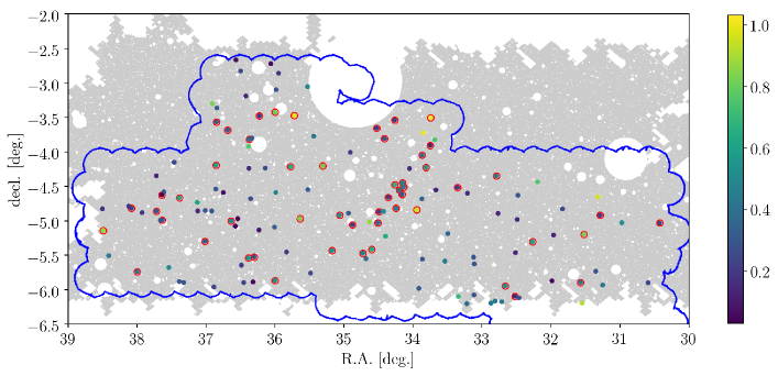
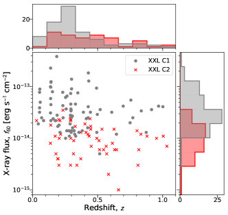
In Table 1 we summarize basic characteristics of the C1+C2, C1, and C2 samples selected for our study. Figure 1 shows the distribution of the full (C1+C2) sample of 136 XXL clusters in the HSC-XMM field (see Section 2.2). Figure 2 shows the distribution of our 136 XXL clusters in the X-ray flux ($f_{60}$) versus redshift ($z$) plane. We summarize in Table 2 the properties of individual clusters in our sample.

2.2. Subaru HSC Survey

We use the HSC first-year shear catalog for our weak-lensing analysis. Full details of the creation of the catalog are described in Mandelbaum et al. (2018a) and Mandelbaum et al. (2018b). We thus refer the reader to those papers and give a basic summary here.

The first-year shear catalog was produced using about 90 nights of HSC-Wide data taken from 2014 March to 2016 April. This shear catalog consists of six distinct patches of the sky covering a total of 137 deg², which is larger than the area covered by the public Data Release 1 (DR1). In this study, we use the shear catalog updated with a star mask called “Arcturus” (Coupon et al., 2018; Miyatake et al., 2019).

HSC-Wide consists of observations made with the $grizy$ filters, reaching a typical limiting magnitude of $i\sim 26$ ABmag ($5\sigma$ for point sources; Aihara et al., 2018a). The $i$-band imaging was performed under exceptional seeing conditions for weak-lensing shape measurements, resulting in a median seeing FWHM of $\simeq 0.6\arcsec$. The galaxy shapes were measured on the co-added $i$-band images using the re-Gaussianization method (Hirata & Seljak, 2003). Basic cuts were applied to select galaxies with robust photometry and shape measurements (Mandelbaum et al., 2018a). The HSC-XMM field covers an effective area of $29.5$ deg² once the star mask region is removed (Figure 1). The area of the overlap region between the HSC and XXL surveys is $21.4$ deg². The weighted number density of source galaxies in the HSC-XMM field is $n_{\mathrm{gal}}\simeq 22.1$ galaxies arcmin^-2, and their mean redshift is $0.82$ (see Miyatake et al., 2019).

We use the HSC multiband photometry to select background source galaxies for a given cluster in the XXL sample. Several different codes were used to estimate photometric redshifts (photo-$z$’s) for individual galaxies from the multiband imaging data (Tanaka et al., 2018). In this work, we employ the point-spread function (PSF) matched aperture (afterburner) photometry (Ephor_AB) code (Tanaka et al., 2018; Hikage et al., 2019). Additional cuts needed to select background source galaxies are described in Section 3.4.

3. HSC Weak-lensing Analysis

3.1. Weak-lensing Basics

The effects of weak gravitational lensing are described by the convergence $\kappa$ and the complex shear $\gamma$. The convergence causes an isotropic magnification, while the shear induces a quadrupole anisotropy that can be estimated from the ellipticities of background galaxies (e.g., Umetsu, 2010). These effects depend on the projected matter overdensity field, as well as on the redshifts of the lens, $z_{l}$, and the source galaxy, $z_{s}$, through the critical surface mass density for lensing, $\Sigma_{\mathrm{cr}}(z_{l},z_{s})$, as defined below. In general, the observable quantity for weak lensing is not $\gamma$, but the reduced shear,

$$g=\frac{\gamma}{1-\kappa}.$$ (1)

The complex shear $\gamma$ can be decomposed into the tangential component $\gamma_{+}$ and the $45^{\circ}$-rotated component $\gamma_{\times}$. The tangential shear component $\gamma_{+}$ averaged around a circle of projected radius $R$ is related to the excess surface mass density $\Delta\Sigma(R)$ through the following identity (Kaiser, 1995):

$$\gamma_{+}(R)=\frac{\Sigma(<R)-\Sigma(R)}{\Sigma_{\mathrm{cr}}(z_{l},z_{s})}\equiv\frac{\Delta\Sigma(R)}{\Sigma_{\mathrm{cr}}(z_{l},z_{s})},$$ (2)

where $\Sigma(R)$ is the azimuthally averaged surface mass density at $R$, $\Sigma(<R)$ denotes the average surface mass density interior to $R$, and

$$\Sigma_{\mathrm{cr}}(z_{l},z_{s})=\frac{c^{2}D_{s}}{4\pi G(1+z_{l})^{2}D_{l}D_{ls}}$$ (3)

with $c$ the speed of light, $G$ the gravitational constant, and $D_{l}$, $D_{s}$ , and $D_{ls}$ the observer–lens, observer–source, and lens–source angular diameter distances, respectively. The extra factor of $(1+z_{l})^{2}$ is due to our use of comoving surface mass densities. The quantity $\Sigma_{\mathrm{cr}}^{-1}(z_{l},z_{s})$ describes the geometric lensing strength, where we set $\Sigma_{\mathrm{cr}}^{-1}(z_{l},z_{s})=0$ for $z_{s}\leqslant z_{l}$.

3.2. Tangential Shear Profile

The X-ray-emitting gas provides an excellent tracer of the total gravitational potential of the cluster (e.g., Donahue et al., 2014; Umetsu et al., 2018; Okabe et al., 2018), except for massive cluster collisions caught in an ongoing phase of dissociative mergers (e.g., Clowe et al., 2006; Okabe & Umetsu, 2008). In this study, we measure the weak-lensing signal around the X-ray peak location of each cluster (Table 2) as a function of comoving cluster-centric radius, $R$. We compute $\Delta\Sigma$ in $N=8$ radial bins of equal logarithmic spacing $\Delta\ln{R}=\ln(R_{\mathrm{max}}/R_{\mathrm{min}})/N\simeq 0.29$ from $R_{\mathrm{min}}=0.3h^{-1}\mathrm{Mpc}$ to $R_{\mathrm{max}}=3h^{-1}\mathrm{Mpc}$ (e.g., Medezinski et al., 2018a; Miyatake et al., 2019). The chosen inner limit $R_{\mathrm{min}}$ is sufficiently large so that our photo-$z$ and shape measurements are not expected to be affected significantly by masking or imperfect deblending by bright cluster galaxies (see discussion in Medezinski et al., 2018b). Moreover, $R_{\mathrm{min}}$ is much larger than the typical offsets between the brightest cluster galaxy (BCG) and the X-ray peak for XXL clusters (Lavoie et al., 2016, hereafter XXL Paper XV). Hence, smoothing of the weak-lensing signal due to miscentering effects (e.g., Johnston et al., 2007; Umetsu et al., 2011a) is expected to be not important for our analysis based on X-ray centering information. However, it should be noted that there is a possibility that a merger has boosted the luminosity and made the X-ray peak off-centered during the compression phase. Although the timescale on which this happens is expected to be short ($\sim 1$ Gyr; see Ricker & Sarazin, 2001; Zhang et al., 2016), it could possibly induce a selection effect and contribute to the scatter in scaling relations.

We estimate $\Delta\Sigma$ in each radial bin for either an individual cluster or a stacked ensemble of multiple clusters using the following estimator (Mandelbaum et al., 2018a):

$$\Delta\Sigma_{+}(R_{i})=\frac{1}{2{\cal R}(R_{i})}\frac{\sum_{l,s\in i}w_{ls}e_{+,ls}[\langle\Sigma_{\mathrm{cr},ls}^{-1}\rangle]^{-1}}{[1+K(R_{i})]\sum_{l,s\in i}w_{ls}},$$ (4)

where the double summation is taken over all clusters of interest ($l$) and over all source galaxies ($s$) that lie within the cluster-centric radial bin ($i$), and

$$e_{+}=-\cos(2\phi)e_{1}-\sin(2\phi)e_{2}$$ (5)

is the tangential ellipticity of the source galaxy, $\phi$ is the angle measured in sky coordinates from the R.A. direction to the line connecting the lens and the source galaxy, and ($e_{1},e_{2}$) are the ellipticity components in sky coordinates obtained from the HSC data analysis pipeline (Mandelbaum et al., 2018a; Bosch et al., 2018). The critical surface mass density for each lens–source pair, $\langle\Sigma_{\mathrm{cr},ls}^{-1}\rangle^{-1}$, is averaged with the photo-$z$ probability distribution function (PDF) of the source galaxy (see Section 3.4), $P_{s}(z)$, as

$$\langle\Sigma_{\mathrm{cr},ls}^{-1}\rangle=\frac{\int_{0}^{\infty}\,P_{s}(z)\Sigma_{\mathrm{cr}}^{-1}(z_{l},z)dz}{\int_{0}^{\infty}\,P_{s}(z)dz}.$$ (6)

The statistical weight factor $w_{ls}$ in Equation (4) is given by

$$w_{ls}=\left(\langle\Sigma_{\mathrm{cr},ls}^{-1}\rangle\right)^{2}\frac{1}{\sigma_{e,s}^{2}+e^{2}_{\mathrm{rms},s}},$$ (7)

where $\sigma_{e,s}$ is the shape measurement uncertainty per ellipticity component (i.e., $\sigma_{e_{1},s}=\sigma_{e_{2},s}\equiv\sigma_{e,s}$) and $e_{\mathrm{rms},s}$ is the rms ellipticity estimate per component. The $[1+K(R_{i})]$ factor statistically corrects for multiplicative residual shear bias as determined from simulations (Mandelbaum et al., 2018a, b),

$$1+K(R_{i})=\frac{\sum_{l,s\in i}w_{ls}(1+m_{s})}{\sum_{l,s\in i}w_{ls}},$$ (8)

where $m_{s}$ denotes the multiplicative bias factor of individual source galaxies. In our ensemble analysis of the XXL sample, we will include a $1\%$ systematic uncertainty on the residual multiplicative bias (see Section 4.2; Mandelbaum et al., 2018b; Hikage et al., 2019). We also conservatively correct for additive residual shear bias by subtracting off the weighted mean offset from Equation (4) (see Mandelbaum et al., 2018a; Miyaoka et al., 2018; Okabe et al., 2019). The shear responsivity ${\cal R}(R_{i})$ is calculated as (see also Mandelbaum et al., 2005b)

$${\cal R}(R_{i})=1-\frac{\sum_{l,s\in i}w_{ls}e^{2}_{\mathrm{rms},s}}{\sum_{l,s\in i}w_{ls}}.$$ (9)

The typical value of ${\cal R}$ is $\approx 0.84$ ($e_{\mathrm{rms}}\approx 0.4$; Medezinski et al., 2018b). A full description and clarification of the procedure are given in Mandelbaum et al. (2018a).

Similarly, we define the $\times$-component surface mass density, $\Delta\Sigma_{\times}$, by replacing $e_{+}$ in Equation (4) with the 45^∘-rotated ellipticity component $e_{\times}$, defined by

$$e_{\times}=-e_{2}\cos{2\phi}+e_{1}\sin{2\phi}.$$ (10)

The azimuthally averaged $\times$ component, or the B-mode signal, is expected to be statistically consistent with zero if the signal is due to weak lensing.

When interpreting the binned tangential shear profile $\mbox{\boldmath$d$}\equiv\{\Delta\Sigma_{+}(R_{i})\}_{i=1}^{N}$, it is important to define and determine the corresponding bin radii $\{R_{i}\}_{i=1}^{N}$ accurately so as to minimize systematic bias in cluster mass measurements. Following Okabe & Smith (2016), we define the effective bin radius $R_{i}$ using the weighted harmonic mean of lens–source transverse separations $R_{ls}$ as

$$R_{i}\equiv\frac{\sum_{l,s\in i}w_{ls}}{\sum_{l,s\in i}w_{ls}R_{ls}^{-1}},$$ (11)

which allows for an unbiased determination of the underlying cluster lensing profile (Okabe & Smith, 2016; Sereno et al., 2017). Similarly, when stacking multiple clusters together, we assume that all the clusters are at a single effective redshift, which is defined as a weighted average over the lens–source pairs used in the stacked analysis,

$$\langle z\rangle_{\mathrm{wl}}=\frac{\sum_{i}\sum_{l,s\in i}w_{ls}z_{l}}{\sum_{i}\sum_{l,s\in i}w_{ls}}.$$ (12)

Figure 3.— Histogram distribution of the weak-lensing SNR, shown separately for the C1 (gray) and C2 (red) subsamples. The median SNR values of the C1 and C2 subsamples are marked by a gray-dashed and a red solid line, respectively. For the full C1+C2 sample, the observed values of weak-lensing SNR span the range from $-2.1$ to $6.0$, with a standard deviation of 1.6.

Finally, to quantify the significance of the shear profile measurement $\mbox{\boldmath$d$}=\{\Delta\Sigma_{+}(R_{i})\}_{i=1}^{N}$ around each individual or stacked cluster, we define a linear signal-to-noise ratio (SNR) estimator (Sereno et al., 2017) by $\mathrm{SNR}=\langle d\rangle/\sigma_{\langle d\rangle}$ with

$$\langle d\rangle= \frac{\sum_{i=1}^{N}\Delta\Sigma_{+}(R_{i})/\sigma^{2}_{\mathrm{shape}}(R_{i})}{\sum_{i=1}^{N}1/\sigma^{2}_{\mathrm{shape}}(R_{i})},$$ (13)

$$\sigma_{\langle d\rangle}= \frac{1}{\sqrt{\sum_{i=1}^{N}1/\sigma^{2}_{\mathrm{shape}}(R_{i})}},$$

and $\sigma_{\mathrm{shape}}(R_{i})$ the statistical uncertainty in Equation (4) due to the shape noise (e.g., Miyaoka et al., 2018),

$$\sigma_{\mathrm{shape}}^{2}(R_{i})=\frac{1}{4{\cal R}^{2}(R_{i})[1+K(R_{i})]^{2}\sum_{l,s\in i}w_{ls}}.$$ (14)

This estimator gives a weak-lensing SNR integrated in the fixed comoving radial range $R\in[0.3,3]\,h^{-1}\mathrm{Mpc}$. We note that we use the full covariance matrix for our cluster mass measurements (Section 3.3).

This SNR estimator is different from the conventional quadratic estimator,

$$(\mathrm{SNR})_{\mathrm{q}}\equiv\left[\sum_{i=1}^{N}(\Delta\Sigma_{+,i})^{2}/\sigma_{\mathrm{shape},i}^{2}\right]^{1/2}>0$$ (15)

(e.g., Umetsu & Broadhurst, 2008; Okabe & Smith, 2016; Lieu et al., 2016, hereafter XXL Paper IV). As noted by Umetsu et al. (2016), this quadratic definition breaks down and leads to overestimation of significance in the noise-dominated regime, in which the actual per-bin SNR is less than unity (see Table 2).

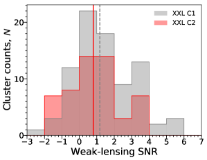
To ensure a statistical ensemble analysis based on weak-lensing measurements of individual clusters, we require the per-cluster SNR to be of the order of unity. Figure 3 shows the histogram distributions of the weak-lensing SNR for the C1 and C2 subsamples. The median per-cluster SNR values for the C1 and C2 subsamples are 1.2 and 0.8, respectively. The median per-cluster SNR of the full (C1+C2) sample is 1.1, so that the above requirement is satisfied.

3.3. Error Covariance Matrix

To obtain robust constraints on the mass scaling relation and its intrinsic scatter, we need to ensure that the mass likelihood from a weak-lensing analysis includes all sources of uncertainty (Gruen et al., 2015). Following Umetsu et al. (2016), we decompose the error covariance matrix for the binned tangential shear profile $d$ as

$$C=C^{\mathrm{shape}}+C^{\mathrm{lss}}+C^{\mathrm{int}},$$ (16)

where $C^{\mathrm{shape}}_{ij}=\sigma^{2}_{\mathrm{shape}}(R_{i})\delta_{ij}$ is the diagonal statistical uncertainty due to the shape noise (see Equation (14)), with $\delta_{ij}$ Kronecker’s delta; $C^{\mathrm{lss}}_{ij}$ is the cosmic noise covariance matrix due to uncorrelated large-scale structures projected along the line of sight (Hoekstra, 2003); and $C^{\mathrm{int}}_{ij}$ accounts for the intrinsic variations of the projected cluster lensing signal at fixed mass due to variations in halo concentration, cluster asphericity, and the presence of correlated halos (Gruen et al., 2015).

We compute the elements of the $C^{\mathrm{lss}}$ matrix by closely following the procedure outlined in Miyaoka et al. (2018) (see also Medezinski et al., 2018a; Miyatake et al., 2019). To this end, we employ the nonlinear matter power spectrum of Smith et al. (2003) for the Wilkinson Microwave Anisotropy Probe (WMAP) 9 yr cosmology (Hinshaw et al., 2013), with a source plane at $z_{s}=1.2$, which closely matches the mean redshift of the selected background galaxies (Medezinski et al., 2018b). When stacking multiple clusters together, we simply scale the $C^{\mathrm{lss}}$ matrix according to the number of independent clusters $N_{\mathrm{cl}}$ as $C^{\mathrm{lss}}\to C^{\mathrm{lss}}/N_{\mathrm{cl}}$ (e.g., Medezinski et al., 2018a).

We estimate the $C^{\mathrm{int}}$ matrix for the tangential shear profile by following Miyatake et al. (2019, see their Appendix), who developed a useful procedure to translate the intrinsic covariance matrix for the convergence (or $\Sigma$) profile (Gruen et al., 2015; Umetsu et al., 2016) to that for the tangential shear (or $\Delta\Sigma$) profile. In the stacked analysis of multiple independent clusters, we scale the $C^{\mathrm{int}}$ matrix as $C^{\mathrm{int}}\to C^{\mathrm{int}}/N_{\mathrm{cl}}$.

As found by Miyatake et al. (2019), the total uncertainty per cluster is dominated by the shape noise ($C^{\mathrm{shape}}$) at $R\lower 2.15277pt\hbox{$\;\buildrel<\over{\sim}\;$}3h^{-1}\mathrm{Mpc}$ (see their Figure 4), beyond which the contribution from the cosmic noise ($C^{\mathrm{lss}}$) becomes important. The relative contribution from intrinsic variance ($C^{\mathrm{int}}$) increases toward the cluster center but remains subdominant at all radii for our weak-lensing measurements.

3.4. Source Galaxy Selection

A secure selection of background galaxies is key for obtaining accurate cluster mass measurements from weak lensing (e.g., Broadhurst et al., 2005; Umetsu & Broadhurst, 2008; Medezinski et al., 2010; Gruen et al., 2014; Okabe & Smith, 2016; Medezinski et al., 2018b). We follow the methodology outlined in Medezinski et al. (2018b) to select background galaxies for our cluster weak-lensing analysis. Two source-selection methods have been tested and established in Medezinski et al. (2018b) using the CAMIRA catalog of optically selected clusters from the HSC survey (Oguri et al., 2018): one based on selection in color-color space (the CC-cut), and another that employs constraints on the cumulative photo-$z$ PDF (the $P$-cut). Both methods are optimized to minimize dilution of the lensing signal and perform comparatively well in removing most of the contamination from foreground and cluster galaxies (Medezinski et al., 2018b). The level of contamination by cluster members depends on and increases with the cluster mass or richness (Medezinski et al., 2018b). For our sample that is dominated by low-mass clusters and groups, we thus expect a less significant degree of dilution of the weak-lensing signal compared to previous HSC cluster weak-lensing studies (e.g., Medezinski et al., 2018b, a; Miyaoka et al., 2018; Miyatake et al., 2019; Okabe et al., 2019).

In the present work, we use the $P$-cut method for our fiducial analysis because it gives higher SNR values (i.e., higher number densities of background galaxies) than the CC-cut method. We use full $P(z)$ data obtained with the Ephor_AB code (Tanaka et al., 2018; Hikage et al., 2019) to define the $P$-cut and to compute the lensing signal (Section 3.2). With this method, for each cluster ($l$), we define a sample of background galaxies ($s=1,2,...$) that satisfy the following conditions (Oguri, 2014; Medezinski et al., 2018b):

$$p_{\mathrm{cut}}<\int_{z_{\mathrm{min},l}}^{\infty}\,P_{s}(z)dz\ \ \ \mathrm{and}\ \ \ z_{\mathrm{p},s}<z_{\mathrm{max}},$$ (17)

where $p_{\mathrm{cut}}$ is a constant probability set to 0.98, $z_{\mathrm{min},l}=z_{l}+\Delta z$ with a constant offset $\Delta z$, $z_{\mathrm{p},s}$ is a photo-$z$ point estimate for the source galaxy, and $z_{\mathrm{max}}$ is the maximum redshift parameter (see Medezinski et al., 2018b). Following Medezinski et al. (2018b), we set $z_{\mathrm{max}}=2.5$ and adopt $\Delta z=0.2$ for a stringent rejection of cluster and foreground galaxies, and we use as $z_{\mathrm{p}}$ a randomly sampled point estimate that is drawn from $P(z)$ (photoz_mc; see Tanaka et al., 2018; Miyatake et al., 2019).

Figure 4.— Stacked surface mass density of the full C1+C2 sample (upper panel) as a function of cluster-centric comoving radius $R$. The results are shown for three different source selection methods. The black squares with error bars show our fiducial results obtained using the $P$-cut method with the Ephor_AB photo-$z$ code. The results obtained using the $P$-cut method with the MLZ code (blue squares) and those using the CC-cut method with the Ephor_AB code (red circles) are shown for comparison. The data points with different selection methods are horizontally shifted with each other for visual clarity. The solid line and the dashed line represent the best-fit NFW model and the halo model (BMO + 2-halo term) derived from the fiducial $P$-cut measurements. The dotted line shows the 2-halo term contribution of the best-fit halo model. The lower panel shows the $45^{\circ}$-rotated shear component $\Delta\Sigma_{\times}$, expected to be consistent with zero.

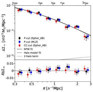
The top panel of Figure 4 shows the stacked tangential shear profiles $\Delta\Sigma_{+}(R)$ obtained for the full sample using the $P$-cut and CC-cut methods, both with the Ephor_AB code. For comparison, we also show the $P$-cut results obtained with MLZ, an unsupervised machine-learning method based on self-organizing maps (SOMs) (Tanaka et al., 2018). The comparison shows no significant difference between these profiles within errors in all bins.

In the bottom panel of Figure 4, we show the corresponding stacked B-model profiles $\Delta\Sigma_{\times}(R)$ (Section 3.2) obtained with these three selection methods. Here we use a $\chi^{2}$ test to assess the significance of the measured B-model signal against the null hypothesis. For our fiducial measurement ($P$-cut with Ephor_AB), we find $\chi^{2}=4.73$ per 8 degrees of freedom (dof). Similarly, we find $\chi^{2}/\mathrm{dof}=5.30/8$ and $\chi^{2}/\mathrm{dof}=4.88/8$ using the $P$-cut method with MLZ and the CC-cut method with Ephor_AB, respectively. In all cases, the B-mode signal is statistically consistent with zero.

In what follows, we focus on the results obtained with the Ephor_AB code. In terms of the best-fit NFW mass model (see Section 4), we find a logarithmic mass offset between the $P$-cut and CC-cut methods of $b_{\mathrm{cont}}\equiv\ln{(M_{\mathrm{500,Pcut}}/M_{500,\mathrm{CC}})}=(+3.1\pm 5.1)\%$, where the error accounts for the covariance between the overlapping source samples. This is consistent with the level of foreground contamination found by Medezinski et al. (2018b). Although we do not find statistical evidence that our $P$-cut method gives a diluted signal compared to the CC-cut method, we conservatively assume a systematic mass uncertainty of $3.1\%$ associated with residual contamination by foreground and cluster galaxies.

3.5. Photometric Redshift Bias

An accurate estimation of photometric redshifts for source galaxies is crucial for weak lensing because biased photo-$z$ estimates can lead to a systematic bias in mass estimates through the calculation of the critical surface density (see Equation (6)). Here we follow the procedure of Miyatake et al. (2019) to quantify the level of this bias. For details of the procedure, we refer to Miyatake et al. (2019, see their Section 3.4).

The photo-$z$ bias in the tangential shear signal of each cluster at redshift $z_{l}$ can be estimated as (Mandelbaum et al., 2008; Nakajima et al., 2012; Miyatake et al., 2019)

$$\frac{\Delta\Sigma}{\Delta\Sigma^{\mathrm{true}}}(z_{l})=1+b_{z}(z_{l})=\frac{\sum_{s}w_{ls}\langle\Sigma^{-1}_{\mathrm{cr},ls}\rangle^{-1}[\Sigma^{\mathrm{true}}_{\mathrm{cr},ls}]^{-1}}{\sum_{s}w_{ls}},$$ (18)

where the quantities with the superscript “true” denote those that would be measured with an unbiased spectroscopic sample, and the sum over $s$ runs over all source galaxies. Ideally, such a photo-$z$ bias should be examined using a spectroscopic-redshift (spec-$z$) sample that is independent from those used to calibrate the photo-$z$’s and that matches the population properties (i.e., magnitude and color distribution) of our source galaxy sample. In practice, however, it is difficult to obtain such a representative spec-$z$ sample matching the depth of our source sample, $i<24.5$ ABmag (Miyatake et al., 2019).

Following Miyatake et al. (2019), we use the 2016 version of the 30-band photo-$z$ catalog of the $2$ deg² COSMOS field (Ilbert et al., 2009; Laigle et al., 2016) as a representative redshift sample and compute the photo-$z$ bias $b_{z}$ for a given cluster redshift, $z_{l}$. As discussed in Hikage et al. (2019, see their Section 5.2), there are some caveats associated with this assumption. We thus use a reweighting method to match the populations between COSMOS galaxies and our background source galaxies (for details, see Hikage et al., 2019; Miyatake et al., 2019). The procedure is summarized as follows. For a given cluster redshift $z_{l}$, we define a sample of background source galaxies from the entire shear catalog using the $P$-cut method described in Section 3.4. We then decompose source galaxies in the weak-lensing sample using their $i$-band magnitude and four colors into cells of an SOM (S. More et al. 2019, in preparation; see Masters et al., 2015). We use a subsample of COSMOS galaxies (Hikage et al., 2019) and classify them into SOM cells defined by the weak-lensing sample and compute their new weights, $w_{\mathrm{SOM}}$, such that the weighted distributions of the photometric observables match those of the corresponding distributions of the weak-lensing sample. We compute the photo-$z$ bias (see Equation (18)) by including $w_{\mathrm{SOM}}$ in the definition of $w_{ls}$.

For our full sample of 136 XXL clusters, we find a weighted average of $\langle b_{z}\rangle\simeq 0.68\%$. We find that our estimate for the average level of photo-$z$ bias is insensitive to the chosen weighting scheme (e.g., a sample median of $\simeq 0.87\%$). The photo-$z$ bias of $\langle b_{z}\rangle\simeq 0.68\%$ is translated into the cluster mass uncertainty as $\langle b_{z}\rangle/\Gamma_{200}\simeq 0.9\%$ with $\Gamma_{200}\equiv d\ln{\Delta\Sigma}/d\ln{M_{200}}\simeq 0.75$, the typical value of the logarithmic derivative of the weak-lensing signal with respect to cluster mass for our cluster weak-lensing analysis (Melchior et al., 2017; Sereno et al., 2017). Hence, the mass calibration uncertainty due to photo-$z$ calibration errors is estimated to be $0.9\%$ (Section 5). Miyatake et al. (2019) found a similar level of photo-$z$ bias ($2\%$) for a sample of eight ACTPol-selected SZE clusters with a median redshift of $z\sim 0.5$.

4. Weighing XXL Clusters

In this section, we use the HSC weak-lensing data to infer the mass and concentration parameters for our XXL cluster sample. In Section 4.1, our procedure for weak-lensing mass modeling is outlined, and the systematic effects in ensemble mass calibration are discussed on the basis of simulations (Appendix A). In Section 4.2, we discuss and summarize systematic errors in ensemble modeling of the XXL sample with weak lensing. Section 4.3 presents our weak-lensing mass estimates of individual clusters in the XXL sample. Section 4.4 presents the results of stacked weak-lensing measurements.

4.1. Mass Modeling

We model the radial mass distribution of galaxy clusters with a spherical NFW profile, which has been motivated by cosmological $N$-body simulations (e.g., Navarro et al., 1996, 1997; Oguri & Hamana, 2011), as well as by direct lensing measurements (e.g., Umetsu et al., 2012, 2014, 2016; Oguri et al., 2012; Newman et al., 2013; Niikura et al., 2015; Okabe & Smith, 2016; Umetsu & Diemer, 2017). The radial dependence of the NFW density profile is given by (Navarro et al., 1996):

$$\rho(r)=\frac{\rho_{\mathrm{s}}}{(r/r_{\mathrm{s}})(1+r/r_{\mathrm{s}})^{2}}$$ (19)

with $\rho_{\mathrm{s}}$ the characteristic density parameter and $r_{\mathrm{s}}$ the characteristic scale radius at which the logarithmic density slope equals $-2$. The overdensity mass $M_{\Delta}$ is given by integrating Equation (19) out to the corresponding overdensity radius $r_{\Delta}$ at which the mean interior density is $\Delta\times\rho_{\mathrm{c}}(z_{l})$ (Section 1), and given as $M_{\Delta}=(4\pi\Delta/3)\rho_{\mathrm{c}}(z_{l})r_{\Delta}^{3}$. We specify the NFW model by the mass, $M_{200}$, and the concentration parameter, $c_{200}=r_{200}/r_{\mathrm{s}}$. The characteristic density $\rho_{\mathrm{s}}$ is then given by

$$\rho_{\mathrm{s}}=\frac{\Delta}{3}\frac{c_{\Delta}^{3}}{\ln(1+c_{\Delta})-c_{\Delta}/(1+c_{\Delta})}\rho_{\mathrm{c}}(z).$$ (20)

We use a Markov Chain Monte Carlo (MCMC) method to obtain well-characterized inference of the mass and concentration parameters from our weak-lensing data (Umetsu et al., 2014, 2016). We adopt log-uniform priors for $M_{200}$ and $c_{200}$ (or uniform priors for $\log{M_{200}}$ and $\log{c_{200}}$) in the range $10^{12}\leqslant M_{200}/(h^{-1}M_{\odot})\leqslant 10^{16}$ and $1\leqslant c_{200}\leqslant 20$.

We note that it is appropriate to assume a log-uniform prior, instead of a uniform prior, for a positive-definite quantity, especially when the quantity spans a wide dynamic range (e.g., Sereno & Covone, 2013; Umetsu et al., 2014, 2016, 2018; Okabe et al., 2019). Such a treatment is also self-consistent with our scaling relation analysis, where we work with logarithmic quantities, $\log{M_{\Delta}}$ and $\log{c_{200}}$ (Section 5). Since the corresponding prior distributions in $M_{200}$ and $c_{200}$ scale as $1/M_{200}$ and $1/c_{200}$, the choice of their lower bounds is relatively important. The chosen priors allow for a sufficiently wide range of mass and concentration relevant for group–cluster-scale halos with $10^{13}h^{-1}M_{\odot}\lower 2.15277pt\hbox{$\;\buildrel<\over{\sim}\;$}M_{200}\lower 2.15277pt\hbox{$\;\buildrel<\over{\sim}\;$}10^{15}h^{-1}M_{\odot}$. If the lower prior boundary of $M_{200}$ is increased toward the mass limit of the sample ($M_{200}\sim 10^{13}h^{-1}M_{\odot}$), this will lead us to overestimate $M_{200}$ for low-mass groups and to underestimate the uncertainty of their mass estimates, owing to the edge effect.

The log-likelihood function for our observations $\mbox{\boldmath$d$}=\{\Delta\Sigma_{+}(R_{i})\}_{i=1}^{N}$ is written as

$$-\ln{\cal L}(\mbox{\boldmath$p$})= \frac{1}{2}\sum_{i,j=1}^{N}\left[\Delta\Sigma_{+}(R_{i})-f_{\mathrm{mod}}(R_{i}|\mbox{\boldmath$p$})\right]$$ (21)

$$\times(C^{-1})_{ij}\left[\Delta\Sigma_{+}(R_{j})-f_{\mathrm{mod}}(R_{j}|\mbox{\boldmath$p$})\right]+\mathrm{const.},$$

where $C^{-1}$ is the inverse covariance matrix and $f_{\mathrm{mod}}(R_{i}|\mbox{\boldmath$p$})$ denotes the theoretical prediction of the model given a set of parameters $\mbox{\boldmath$p$}=(M_{200},c_{200})$. We use analytic expressions given by Wright & Brainerd (2000) for the radial dependence of the projected NFW profiles $\Sigma_{\mathrm{NFW}}(R|\mbox{\boldmath$p$})$ and $\Delta\Sigma_{\mathrm{NFW}}(R|\mbox{\boldmath$p$})$, which provide a good approximation for the projected matter distribution around clusters (Oguri & Hamana, 2011). The contribution from the 2-halo term to $\Delta\Sigma$ becomes significant at about several virial radii (Oguri & Hamana, 2011), which is larger than the outer radial limit, $R_{\mathrm{max}}=3h^{-1}\mathrm{Mpc}$ (see also Section 4.4). We thus fit the tangential shear profile $\mbox{\boldmath$d$}=\{\Delta\Sigma_{+}(R_{i})\}_{i=1}^{N}$ over the full radial range $R\in[0.3,3]\,h^{-1}\mathrm{Mpc}$ in comoving length units.

Since the relation between the observable image distortion and the lensing fields is nonlinear (see Equation (1)), the observed $\Delta\Sigma$ profile is nonlinearly related to the averaged lensing fields. Here we use the following approximation to include next-to-leading-order corrections (Umetsu et al., 2014):

$$f_{\mathrm{mod}}(R_{i}|\mbox{\boldmath$p$}) =\frac{\Delta\Sigma_{\mathrm{NFW}}(R_{i}|\mbox{\boldmath$p$})}{1-\langle\!\langle\Sigma_{\mathrm{cr},i}^{-1}\rangle\!\rangle\times\Sigma_{\mathrm{NFW}}(R_{i}|\mbox{\boldmath$p$})},$$ (22)

where $\langle\!\langle\Sigma_{\mathrm{cr},i}^{-1}\rangle\!\rangle$ is the sensitivity-weighted, inverse critical surface mass density evaluated in each radial bin, defined by

$$\langle\!\langle\Sigma_{\mathrm{cr},i}^{-1}\rangle\!\rangle=\frac{\sum_{l,s\in i}w_{ls}\langle\Sigma_{\mathrm{cr},ls}^{-1}\rangle}{\sum_{l,s\in i}w_{ls}}.$$ (23)

As summary statistics, we employ the biweight estimator of Beers et al. (1990) to represent the center location ($C_{\mathrm{BI}}$) and the scale or spread ($S_{\mathrm{BI}}$) of marginalized one-dimensional posterior distributions (e.g., Stanford et al., 1998; Sereno & Umetsu, 2011; Biviano et al., 2013; Umetsu et al., 2014, 2016, 2018). Biweight statistics are insensitive to and stable (robust) against noisy outliers because they assign higher weights to data points that are closer to the center of the distribution (Beers et al., 1990). For a lognormally distributed quantity, $C_{\mathrm{BI}}$ approximates the median of the distribution. From the posterior samples, we derive marginalized constraints on the total mass $M_{\Delta}$ and the concentration $c_{\Delta}$ at several characteristic interior overdensities $\Delta$.

Our modeling procedure and assumptions have been tested and validated with simulations. In Appendix A, we describe the details of tests of our “shear-to-mass” procedure and pipeline. There are two possible main sources of systematics in an ensemble weak-lensing analysis of the XXL sample that includes low-mass groups: modeling of those groups/clusters detected with low values of weak-lensing SNR (Figure 3), and the modeling uncertainty due to systematic deviations from the assumed NFW form in projection. To this end, we use two different sets of simulations to assess the impact of these systematic effects. To examine the first possibility (Appendix A.1), we analyze synthetic weak-lensing data based on simulations of analytical NFW lenses. These simulations closely match our weak-lensing observations in terms of the noise level and the SNR distribution. To address the second possibility (Appendix A.2), we analyze a set of synthetic data created from a DM-only realization of BAHAMAS simulations (McCarthy et al., 2017).

Our simulations show that the overall mass scale of a sample of XXL-like clusters can be recovered within $3.3\%$ accuracy from individual cluster weak-lensing measurements (Appendix A). Specifically, we find the level of mass bias (see Equation (A1)) to be $b_{\mathrm{sim},M_{200}}=(2.1\pm 1.5)\%$ and $b_{\mathrm{sim},M_{500}}=(0.9\pm 1.3)\%$ in $M_{200}$ and $M_{500}$, respectively, with the BAHAMAS simulation (Appendix A.2). With synthetic data from simulations of NFW lenses (Appendix A.1), we find $b_{\mathrm{sim},M_{200}}=(0.1\pm 2.4)\%$ and $b_{\mathrm{sim},M_{500}}=(3.3\pm 2.3)\%$, with no systematic dependence on cluster mass over the full range in true cluster mass (Figure 13).

However, the results from the BAHAMAS simulation suggest a significant level of mass bias of $\sim-20\%$ for low-mass group systems with $M_{\mathrm{200,true}}\lower 2.15277pt\hbox{$\;\buildrel<\over{\sim}\;$}4\times 10^{13}h^{-1}M_{\odot}$ (Appendix A.2; see Table 6). Since we do not find any mass-dependent behavior when using the true density profile assumed in our simulations of NFW lenses, it is likely that this negative bias is caused by systematic deviations of “projected” halos from the NFW profile shape. In fact, we find such a systematic trend in the outskirts ($1\lower 2.15277pt\hbox{$\;\buildrel<\over{\sim}\;$}R/r_{200}\lower 2.15277pt\hbox{$\;\buildrel<\over{\sim}\;$}3$) of projected $\Delta\Sigma(R)$ profiles around low-mass group-scale halos selected from DM-only BAHAMAS simulations, whereas their spherically averaged density profiles $\rho(r)$ in three dimensions are well described by the NFW form (M. Lieu et al. 2020, in preparation). However, we note that the typical mass measurement uncertainty for such low-mass groups is $\sigma(M)/M\sim 140\%$ per cluster (see Appendix A.1), and that even when averaging over all such clusters, the statistical uncertainty on the mean mass is of the order of $\lower 2.15277pt\hbox{$\;\buildrel>\over{\sim}\;$}20\%$ (Section 4.3). This level of systematic bias ($\lower 2.15277pt\hbox{$\;\buildrel<\over{\sim}\;$}1\sigma$) is not expected to significantly affect our ensemble weak-lensing analysis of the XXL sample.

On the other hand, we find a significant systematic offset in the mean concentration recovered from weak lensing: $b_{\mathrm{sim},c_{200}}=(-18\pm 2)\%$ from the BAHAMAS simulation and $b_{\mathrm{sim},c_{200}}=(13\pm 3)\%$ from our simulations of NFW lenses. This is because the typical scale radius for our sample, $r_{\mathrm{s}}\sim 0.25h^{-1}\mathrm{Mpc}$, lies slightly below the radial range for fitting, $R\in[0.3,3]\,h^{-1}\mathrm{Mpc}$ (comoving), and the characteristic profile curvature around $r_{\mathrm{s}}$ is poorly constrained by our data.

4.2. Systematic Uncertainties in Ensemble Modeling

We have accounted for various sources of statistical errors associated with cluster weak-lensing measurements (Section 3.3). All of these errors are encoded in the total covariance matrix $C=C^{\mathrm{shape}}+C^{\mathrm{lss}}+C^{\mathrm{int}}$ (see Equation (16)) of the binned tangential shear profile, $\mbox{\boldmath$d$}=\{\Delta\Sigma_{+}(R_{i})\}_{i=1}^{N}$ (Section 3.2). We have statistically corrected our tangential shear measurements for multiplicative and additive residual shear bias estimated from the dedicated image simulations (Section 3.2; see Mandelbaum et al., 2018b, a).

We have also quantified unaccounted-for sources of systematic errors in cluster mass calibration by considering the following effects: (i) the residual systematic uncertainty in the overall shear calibration (Section 3.2), $1\%$; (ii) dilution of the weak-lensing signal by residual contamination from foreground and cluster members (Section 3.4), $b_{\mathrm{cont}}\simeq 3.1\%$; (iii) photo-$z$ bias in the $\langle\Sigma_{\mathrm{cr}}^{-1}\rangle$ estimates (Section 3.5), $\langle b_{z}\rangle/\Gamma\simeq 0.9\%$; and (iv) the systematic uncertainty in the overall mass modeling (Section 4.1), $b_{\mathrm{sim}}\simeq 3.3\%$. These systematic errors add up in quadrature to a total systematic uncertainty of $\simeq 5\%$ in the ensemble mass calibration of the XXL sample. This level of systematic uncertainty is below the statistical precision of the current full sample, $\simeq 9\%$ at $M_{200}\sim 9\times 10^{13}h^{-1}M_{\odot}$ (Table 1). We account for these systematics and marginalize over the mass calibration uncertainty of $\pm 5\%$ in our scaling relation analyses (Section 5).

Regarding the concentration parameter, since we find systematic errors of opposite signs from the two sets of simulations (Section 4.1), we include a systematic uncertainty of $\pm\sqrt{(0.18^{2}+0.13^{2})/2}\simeq\pm 16\%$ (Appendix A) on the normalization of the $c$–$M$ relation (Section 5.2). Possible sources of bias are the mass-dependent deviations from the NFW form, the effect of correlated structure, and noise. All these are functions of the projected cluster-centric radius, and the net effect is sensitive to the radial fitting range. We note that the level of systematic errors in $c_{200}$ is below the statistical uncertainty, even for our ensemble measurements of the XXL sample (see Equation (40) and Table 1).

4.3. Individual Cluster Weak-lensing Analysis

In Table 2 we list posterior summary statistics ($C_{\mathrm{BI}}\pm S_{\mathrm{BI}}$ and median values) of the mass and concentration parameters $(c_{200},M_{200},M_{500})$ for all individual clusters in the full C1+C2 sample.

There are 31 clusters whose weak-lensing SNR values are negative as dominated by statistical noise fluctuations (Table 2; see also Sereno et al., 2017). These clusters span a wide range of redshift ($0.044\leqslant z\leqslant 0.953$) with a median of $0.324$. The typical mass uncertainty for these clusters is $S_{\mathrm{BI}}/C_{\mathrm{BI}}\sim 140\%$, so that their mass estimates are consistent with zero. According to our simulations based on analytical NFW lenses, such low SNR clusters are distributed over a fairly representative range in true mass (Appendix A.1; see Figures 11 and 12). At a given true mass, it is expected that there is a statistical counterpart of up-scattered clusters with apparently boosted SNR values and thus overestimated weak-lensing masses. In fact, the simulations show that the inclusion of low-SNR clusters does not significantly bias our ensemble mass measurements at particular mass scales (see Figure 13). It must be stressed that if one selects a subsample of clusters according to their weak-lensing SNR values, they are no more representative of the parent population, and such a selection will bias high the weak-lensing mass estimates at a given X-ray cut, an effect known as the Malmquist bias (e.g., Sereno & Ettori, 2017, see also Appendix A.1).

As a robust estimator for the average $M_{\Delta}$ over a given cluster sample ($n=1,2,...,N_{\mathrm{cl}}$), we use geometric means, instead of arithmetic means. An advantage of using this geometric estimator is that error-weighted geometric means of cluster properties, such as $M_{200}$ and $c_{200}$, are relevant to our scaling relation analysis, where we work with logarithmic quantities (Section 5). Specifically, we employ an error-weighted, geometric mean estimator for the sample average (Umetsu et al., 2014, 2016; Okabe & Smith, 2016), defined by

$$\langle M_{\Delta}\rangle_{\mathrm{g}}:=e^{\langle\ln M_{\Delta}\rangle}=\exp{\left(\frac{\sum_{n=1}^{N_{\mathrm{cl}}}u_{n}\ln{M_{\Delta,n}}}{\sum_{n}u_{n}}\right)}$$ (24)

and its uncertainty,

$$\sigma_{\langle M_{\Delta}\rangle_{\mathrm{g}}} =\frac{1}{2}\langle M_{\Delta}\rangle_{\mathrm{g}}$$ (25)

$$\times \left[\exp\left(\frac{1}{\sqrt{\sum_{n=1}^{N_{\mathrm{cl}}}u_{n}}}\right)-\exp\left(-\frac{1}{\sqrt{\sum_{n=1}^{N_{\mathrm{cl}}}u_{n}}}\right)\right],$$

where $u_{n}$ is the inverse variance weight for the $n$th cluster, $u_{n}^{-1}=\sigma^{2}(M_{\Delta,n})/M_{\Delta,n}^{2}$, with $M_{\Delta,n}$ and $\sigma(M_{\Delta,n})$ being $C_{\mathrm{BI}}$ and $S_{\mathrm{BI}}$ (Section 4.1), respectively, of the marginalized posterior distribution of $M_{\Delta}$ for the $n$th cluster. The geometric means are symmetric with respect to an exchange of the numerator and denominator (i.e., $\langle A/B\rangle_{\mathrm{g}}=\langle B/A\rangle_{\mathrm{g}}^{-1}$), so that this weighted geometric estimator is also suitable for use in estimating mean mass ratios between two cluster samples (Donahue et al., 2014; Umetsu et al., 2014, 2016).

Using this estimator, we find weighted geometric means of $\langle M_{200}\rangle_{\mathrm{g}}=(9.8\pm 0.8)\times 10^{13}h^{-1}M_{\odot}$, $\langle M_{200}\rangle_{\mathrm{g}}=(11.6\pm 1.2)\times 10^{13}h^{-1}M_{\odot}$, and $\langle M_{200}\rangle_{\mathrm{g}}=(6.5\pm 1.0)\times 10^{13}h^{-1}M_{\odot}$ for the C1+C2, C1, and C2 samples, respectively (Table 1).

4.4. Stacked Weak-lensing Analysis

Stacking an ensemble of clusters helps average out large statistical fluctuations inherent in noisy weak-lensing measurements of individual clusters (Section 3.3). The statistical precision can be greatly improved by stacking together a large number of clusters, allowing for tighter and more robust constraints on the cluster mass distribution. A stacked analysis is complementary to our primary approach based on individual weak-lensing mass measurements. A comparison of the two approaches thus provides a useful consistency check in different SNR regimes. It is noteworthy, however, that interpreting the effective mass from stacked lensing requires caution because the amplitude of the lensing signal is weighted by the redshift-dependent sensitivity (Umetsu et al., 2016) and is not linearly proportional to the cluster mass (Mandelbaum et al., 2005a; Melchior et al., 2017; Sereno et al., 2017; Miyatake et al., 2019).

Table 3 Characteristics of the $T_{\mathrm{X}}$-binned Subsamples

Bin	$N_{\mathrm{cl}}$	$T_{\mathrm{X}}$	$\langle T_{\mathrm{X}}\rangle_{\mathrm{wl}}$	$z$	$\langle z\rangle_{\mathrm{wl}}$	$c_{200}$	$M_{200}$	$\langle M_{200}\rangle_{\mathrm{wl}}$	$\langle M_{200}\rangle_{\mathrm{g}}$	SNR	$($SNR$)_{\mathrm{q}}$
		(keV)	(keV)				($10^{13}h^{-1}M_{\odot}$)	($10^{13}h^{-1}M_{\odot}$)	($10^{13}h^{-1}M_{\odot}$)
T1	$22$	$1.1$	$1.0$	$0.18$	$0.18$	$5.7\pm 4.6$	$4.5\pm 1.2$	$4.8\pm 1.4$	$4.1\pm 1.0$	$5.3$	$7.9$
T2	$21$	$1.6$	$1.5$	$0.29$	$0.22$	$3.2\pm 1.9$	$8.3\pm 1.9$	$6.5\pm 1.7$	$7.9\pm 1.8$	$6.9$	$9.1$
T3	$17$	$1.9$	$1.9$	$0.30$	$0.29$	$3.0\pm 1.4$	$12.6\pm 2.7$	$9.5\pm 2.2$	$13.6\pm 3.0$	$6.6$	$9.5$
T4	$19$	$2.4$	$2.4$	$0.33$	$0.31$	$2.0\pm 1.0$	$11.3\pm 3.0$	$8.0\pm 2.4$	$6.7\pm 1.8$	$6.2$	$7.9$
T5	$17$	$3.5$	$3.4$	$0.43$	$0.33$	$4.3\pm 2.4$	$19.8\pm 4.1$	$19.6\pm 4.4$	$20.2\pm 4.1$	$8.7$	$10.4$
T6	$9$	$5.0$	$5.1$	$0.51$	$0.31$	$5.9\pm 3.0$	$25.8\pm 5.3$	$22.6\pm 5.2$	$25.8\pm 5.7$	$7.3$	$10.2$

Note. — The definitions of the columns are the same as in Table 1.

Figure 5.— Stacked weak-lensing constraints on the NFW concentration and mass parameters (circles with error bars) for six subsamples of our XXL clusters (see Table 3) binned in X-ray temperature. This analysis is limited to 105 C1+C2 clusters with measured X-ray temperatures $T_{\mathrm{300\,kpc}}$ from the XXL survey. The X-ray temperature of the data points is color-coded according to the color bar on the right side. The black square with error bars shows the weighted average of individual weak-lensing measurements over the sample of 105 XXL clusters. The results are compared to theoretical $c$–$M$ relations evaluated at $z=0.3$ for the full population of DM halos from numerical simulations of $\Lambda$CDM cosmologies (Bhattacharya et al., 2013; Child et al., 2018; Diemer & Joyce, 2019). The gray shaded region represents the lognormal intrinsic dispersion $\sigma(\ln{c_{200}})=1/3$ around the $c$–$M$ relation of Bhattacharya et al. (2013).

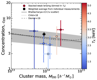
First, we examine the effective mass and concentration parameters of the full C1+C2 sample of 136 XXL clusters from the stacked $\Delta\Sigma$ profile shown in Figure 4 (fiducial). The lensing-weighted mean redshift of the full sample is $\langle z\rangle_{\mathrm{wl}}\simeq 0.25$, which is smaller than the sample median redshift, $z=0.30$. From a single-mass-bin NFW fit to the stacked $\Delta\Sigma$ profile (see Section 4), we obtain $M_{200}=(8.7\pm 0.8)\times 10^{13}h^{-1}M_{\odot}$ and $c_{200}=3.5\pm 0.9$ for the C1+C2 sample. This is in agreement with the degree of concentration expected for DM halos in the standard $\Lambda$CDM cosmology, $c_{200}\simeq 4.1$ at $M_{200}=8.7\times 10^{13}h^{-1}M_{\odot}$ and $z=0.25$ (Diemer & Kravtsov, 2015; Diemer & Joyce, 2019). The effective mass and concentration parameters for the C1+C2, C1, and C2 samples are summarized in Table 1.

In Figure 4, we also show the best-fit two-parameter halo model including the effects of surrounding large-scale structure as a 2-halo term. Here we follow the standard halo model prescription of Oguri & Hamana (2011) using the linear halo bias $b_{\mathrm{h}}(M_{200};z)$ of Tinker et al. (2010) in a WMAP 9 yr based $\Lambda$CDM cosmology (Hinshaw et al., 2013). The 2-halo term contribution to the $\Delta\Sigma(R)$ profile in comoving length units is expressed as

$$\Delta\Sigma_{\mathrm{2h}}(R)=\frac{\rho_{\mathrm{m}}(z)b_{\mathrm{h}}(M_{200};z)}{(1+z)^{3}d_{\mathrm{A}}^{2}(z)}\int\!\frac{ldl}{2\pi}\,J_{2}(l\theta)P(k_{l};z),$$ (26)

where $\rho_{\mathrm{m}}(z)$ is the mean matter density of the universe at the cluster redshift $z$, $d_{\mathrm{A}}(z)$ is the comoving angular diameter distance, $P(k;z)$ is the linear matter power spectrum, $k_{l}\equiv l/d_{\mathrm{A}}(z)$, $\theta\equiv R/d_{\mathrm{A}}(z)$, and $J_{n}$ is the Bessel function of the first kind and $n$th order. The 2-halo term is proportional to the product $b_{\mathrm{h}}\sigma_{8}^{2}$.

As demonstrated in Figure 4, the 2-halo term $\Delta\Sigma_{\mathrm{2h}}(R)$ in the radial range $R\in[0.3,3]\,h^{-1}\mathrm{Mpc}$ is negligibly small, even in low-mass groups (see Leauthaud et al., 2010; Covone et al., 2014; Sereno et al., 2015b, 2017). This is because the tangential shear, or the excess surface mass density $\Delta\Sigma(R)=\Sigma(<R)-\Sigma(R)$, is insensitive to flattened sheet-like structures (Schneider & Seitz, 1995). When the 2-halo term is neglected, the standard halo model reduces to the Baltz–Marshall–Oguri (Baltz et al., 2009, BMO) model that describes a smoothly truncated NFW profile (Umetsu et al., 2016, see their Section 5.2.2). Using synthetic weak-lensing data based on the DM-only BAHAMAS simulation (Appendix A.2), we find that the standard halo modeling does not significantly improve the accuracy of weak-lensing mass estimates for a sample of XXL-like objects (see Table 6).

As a consistency check of our ensemble weak-lensing analysis, we compare the stacked lensing constraints on $M_{200}$ with those from individual cluster measurements (see Section 4.3). It is reassuring that the effective $M_{200}$ masses extracted from the stacked $\Delta\Sigma$ profiles are in good agreement with the respective weighted geometric means $\langle M_{200}\rangle_{\mathrm{g}}$ obtained from individual cluster mass estimates (see Table 1). Alternatively, we can estimate the average mass by using the lensing weight to be consistent with the stacked weak-lensing analysis (see Equation 4; Umetsu et al., 2016; Medezinski et al., 2018a; Miyatake et al., 2019) as

$$\langle M_{\Delta}\rangle_{\mathrm{wl}}=(\sum_{l,s}w_{ls})^{-1}\sum_{l}M_{\Delta,l}\sum_{s}w_{ls}.$$ (27)

Incorporating the lens weighting, we find $\langle M_{200}\rangle_{\mathrm{wl}}=(8.0\pm 0.8)\times 10^{13}h^{-1}M_{\odot}$, $(9.0\pm 1.0)\times 10^{13}h^{-1}M_{\odot}$, and $(6.1\pm 1.1)\times 10^{13}h^{-1}M_{\odot}$ for the C1+C2, C1, and C2 samples, respectively, all consistent with the results from the stacked analysis within the errors (see Table 1). This agreement suggests that those clusters detected with low values of weak-lensing SNR are not biasing the ensemble-averaged mass with respect to the stacked weak-lensing analysis.

Next, we perform a stacked analysis by dividing the full sample into 6 subsamples with roughly equal numbers (except for the highest temperature bin) according to the X-ray temperature, $T_{\mathrm{300\,kpc}}$. This analysis is limited to 105 clusters with measured X-ray temperatures $T_{\mathrm{300\,kpc}}$ from the XXL survey (Section 2.1). This subsample has a weighted average mass of $\langle M_{200}\rangle_{\mathrm{g}}=(8.6\pm 0.9)\times 10^{13}h^{-1}M_{\odot}$ and a weighted average concentration of $\langle c_{200}\rangle_{\mathrm{g}}=4.8\pm 0.4\,(\mathrm{stat.})\pm 0.8\,(\mathrm{syst.})$ (Figure 5).

The results of stacked weak-lensing measurements are summarized in Table 3. These subsamples have similar SNR values, ranging from 5.3 to 8.7, with a median of 6.7. For each subsample, we derive $(M_{200},c_{200})$ from a single-mass-bin fit to the stacked $\Delta\Sigma$ profile. The mass extracted from the stacked lensing signal ranges from $M_{200}=(4.5\pm 0.9)\times 10^{13}h^{-1}M_{\odot}$ at $T_{\mathrm{300\,kpc}}\simeq 1.0$ keV to $M_{200}=(2.6\pm 0.3)\times 10^{14}h^{-1}M_{\odot}$ at $T_{\mathrm{300\,kpc}}\simeq 5.2$ keV. The effective $M_{200}$ mass extracted from the stacked analysis and the corresponding lensing-weighted mass $\langle M_{200}\rangle_{\mathrm{wl}}$ from individual cluster measurements are consistent within the errors in all $T_{\mathrm{300\,kpc}}$ bins (Table 3). Overall, these lensing-weighted mass estimates are in agreement with the error-weighted geometric means $\langle M_{200}\rangle_{\mathrm{g}}$ from individual cluster mass estimates (Tables 1 and 3).

In Figure 5 we show the distribution of $(M_{200},c_{200})$ for the six subsamples along with with theoretical predictions for the full population of $\Lambda$CDM halos (Bhattacharya et al., 2013; Child et al., 2018; Diemer & Joyce, 2019). All these models are evaluated at a reference redshift of $z_{\mathrm{ref}}=0.3$ and designed for a qualitative comparison and a consistency check only (see Table 3). The average X-ray temperature of each subsample is color-coded according to the color bar on the right side. Figure 5 shows that $M_{200}$ correlates well with $T_{\mathrm{300\,kpc}}$, and that $c_{200}$ is scattered around the theoretical $c$–$M$ relations, with no hint of significant overconcentration for the XXL sample. A complete regression analysis of the $c$–$M$ relation, accounting for various statistical effects, is given in Section 5.2.

5. XXL Mass Scaling Relations

In this section we examine and characterize the concentration–mass ($c_{200}$–$M_{200}$) and temperature–mass ($T_{\mathrm{300\,kpc}}$–$M_{500}$) scaling relations separately for the XXL sample using our HSC and XXL data products presented in the previous sections.

5.1. Bayesian Regression Scheme

Here we outline the Bayesian regression scheme of Sereno (2016a) used in our scaling relation analysis. Our regression approach allows for a self-consistent treatment of redshift evolution, intrinsic scatter, and selection effects through Bayesian population modeling of the cluster sample. For full details of the formalism, we refer the reader to Sereno (2016a) and the companion paper by Sereno et al. (2020).

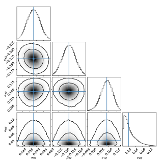
In this analysis, we use the publicly available LIRA package (Sereno, 2016a, b). We have tested and validated our analysis procedure and its LIRA implementation by performing a regression analysis of the $c_{200}$–$M_{200}$ relation using realistic synthetic data based on the DM-only BAHAMAS simulation (see Appendix A.2). We find that we can accurately recover the true (input) parameters of the $c_{200}$–$M_{200}$ relation except for the normalization, which is subject to a systematic offset (see Section 4.2 and Appendix A).

5.1.1 Mass Scaling Relations

We consider a power-law function of the following form that describes the average mass scaling relation of a given cluster observable ${\cal O}$:

$${\cal O}\propto 10^{\alpha}M_{\Delta}^{\beta}F_{z}(z)^{\gamma},$$ (28)

where $\alpha$, $\beta$, and $\gamma$ denote the normalization, mass trend, and redshift trend, respectively; $F_{z}(z)$ describes the redshift evolution of the scaling relation and is normalized to unity at a reference redshift, $z_{\mathrm{ref}}$. In this work, we consider $F_{z}(z)=(1+z)/(1+z_{\mathrm{ref}})$ for the $c_{200}$–$M_{200}$ relation (e.g., Duffy et al., 2008; Dutton & Macciò, 2014) and $F_{z}(z)=E(z)/E(z_{\mathrm{ref}})$ for the $T_{\mathrm{300\,kpc}}$–$M_{500}$ relation (e.g., Vikhlinin et al., 2009a; Ettori, 2015; Mantz et al., 2016). In what follows, we set $z_{\mathrm{ref}}=0.3$.

We focus on the logarithms of quantities that describe global cluster properties of interest. These logarithmic quantities are then linearly related to each other. We consider the cluster mass $M_{\Delta}$ as the most fundamental property of galaxy clusters and define the corresponding logarithmic quantity as

$$Z=\log{\left(\frac{M_{\Delta}}{M_{\Delta,\mathrm{pivot}}}\right)}$$ (29)

with $M_{\Delta,\mathrm{pivot}}$ the pivot in the $M_{\Delta}$ mass. We use the weak-lensing mass $M_{\Delta,\mathrm{wl}}$ as a mass proxy and introduce the logarithmic weak-lensing mass,

$$X=\log{\left(\frac{M_{\Delta,\mathrm{WL}}}{M_{\Delta,\mathrm{pivot}}}\right)}.$$ (30)

For a regression analysis of the $c_{200}$–$M_{200}$ relation, we choose the pivot in $M_{200}$ to be $M_{200,\mathrm{pivot}}=10^{14}h^{-1}M_{\odot}$ and define the logarithmic observable,

$$Y=\log{c_{200}}.$$ (31)

For the $T_{\mathrm{300\,kpc}}$–$M_{500}$ relation, we set $M_{500,\mathrm{pivot}}=7\times 10^{13}h^{-1}M_{\odot}=10^{14}M_{\odot}$ and define

$$Y=\log{\left(\frac{T_{\mathrm{300\,kpc}}}{1\,\mathrm{keV}}\right)}.$$ (32)

For any observable cluster property, we distinguish the following three quantities: (i) $Y_{Z}$, the quantity that is exactly linked to $Z$ through a deterministic functional relation $Y_{Z}(Z)$ (Maughan, 2014); (ii) $Y$, a scattered version of $Y_{Z}$; and (iii) $y$, a measured realization of $Y$ that includes observational noise. As defined, $Y$ is intrinsically scattered with respect to $Y_{Z}$, which we may express as $Y=Y_{Z}(Z)\pm\sigma_{Y|Z}$, with $\sigma_{Y|Z}$ the intrinsic dispersion of $Y$ at fixed cluster mass or $Z$.

To proceed, we assume that the weak-lensing mass ($X$) is an unbiased but scattered proxy of the true cluster mass ($Z$). The mass scaling relations $Y_{Z}(Z)$ and $X_{Z}(Z)$ are then expressed as

$$Y_{Z} = \alpha_{Y|Z}+\beta_{Y|Z}Z+\gamma_{Y|Z}\log{F_{z}(z)},$$ (33)

$$X_{Z} = Z,$$ (34)

where $\alpha_{Y|Z}$, $\beta_{Y|Z}$, and $\gamma_{Y|Z}$ are the intercept, mass-trend, and redshift-trend parameters, respectively. We may rewrite Equation (34) as $X=Z\pm\sigma_{X|Z}$ with $\sigma_{X|Z}$ the intrinsic dispersion of $X$ at fixed $Z$.

5.1.2 Mass Calibration Uncertainty

Any mass calibration bias (i.e., $Z_{X}=\alpha_{Z|X}+X$ with $\alpha_{X|Z}\neq 0$) can lead to a biased estimate of the normalization of the scaling relation, $\alpha_{Y|Z}$. We assume a zero-centered Gaussian prior on $\alpha_{X|Z}$ of $\alpha_{X|Z}=\pm 5\%/\ln{10}$ to marginalize over the remaining mass calibration uncertainty of $\pm 5\%$ (see Section 4.2).

5.1.3 Measurement Errors

The measured quantities $x$ and $y$ are noisy realizations of the latent variables $X$ and $Y$, respectively. We assume that the measurement errors for the two cluster observables ($X,Y$) follow a bivariate Gaussian distribution (Sereno, 2016a).

In the XXL survey, the X-ray temperature $T_{\mathrm{300\,kpc}}$ was measured in a fixed aperture of 300 kpc (XXL Paper II). The errors in the X-ray temperature $T_{\mathrm{300\,kpc}}$ and the weak-lensing mass $M_{\Delta,\mathrm{WL}}$ are thus independent of each other.

On the other hand, for a given cluster, the measurement errors between the NFW parameters are correlated (Section 4.1). For the regression of the $c_{200}$–$M_{200}$ relation, we thus compute the error covariance matrix of the $(\log{M_{\mathrm{200,WL}}},\log{c_{200}})$ parameters using the MCMC posterior samples (see Section 4.1) and account for the covariance between the two parameters (e.g., Umetsu et al., 2014, 2016; Okabe & Smith, 2016). We note that the correlation coefficient $r_{\mathrm{CC}}(\log{M_{\mathrm{200,WL}}},\log{c_{200}})$ between the two NFW parameters is close to zero on average $(\langle r_{\mathrm{CC}}\rangle\sim-0.03)$ for clusters with noisy weak-lensing measurements ($\mathrm{SNR}<1$), so that the two parameters are nearly independent in the low-SNR regime. The correlation coefficient becomes more negative with increasing weak-lensing SNR (and with increasing $M_{\mathrm{200,WL}}$; see the right panel of Figure 12), reaching $r_{\mathrm{CC}}\sim-0.6$ at $\mathrm{SNR}\sim 5$.

5.1.4 Intrinsic Scatter

The true cluster properties ($X,Y$), which one would measure in a hypothetical noiseless experiment, are intrinsically scattered with respect to ($X_{Z},Y_{Z}$) (Sereno, 2016a). We assume that the intrinsic scatter of the true quantity ($X$ or $Y$) around its model prediction ($X_{Z}$ or $Y_{Z}$) at fixed $Z$ follows a Gaussian distribution. For a given observable–mass relation (i.e., $c_{200}$–$M_{200}$ or $T_{\mathrm{300\,kpc}}$–$M_{500}$), we have two intrinsic dispersion parameters, $\sigma_{Y|Z}$ and $\sigma_{X|Z}$, which are assumed to be constant with mass and redshift.

5.1.5 Intrinsic Distribution and Selection Effects

A proper modeling of the mass probability distribution $P(Z)$ is crucial. Cluster samples are usually biased with respect to the underlying parent population (i.e., the mass function) because clusters are selected according to their observable properties. Moreover, even in absence of selection effects, the parent population is not uniformly distributed in logarithmic mass $Z$, which can cause tail effects (e.g., Kelly, 2007).

The intrinsic distribution of the selected clusters is mainly shaped by the following two effects: first, as predicted by the mass function, more massive objects are rarer; second, less massive objects are typically fainter and more difficult to detect. Accordingly, the resulting mass probability distribution tends to be unimodal, and it evolves with redshift (Sereno & Ettori, 2015a).

The combined evolution of the completeness and the mass function can be modeled through the evolution of the mean and dispersion of the effective mass probability distribution. In general, the intrinsic mass probability distribution $P(Z)$ of the selected clusters can be approximated with a mixture of time-evolving Gaussian functions (Kelly, 2007; Sereno et al., 2015a; Sereno & Ettori, 2015a).

We properly account for these effects and Eddington bias in Bayesian regression. In this work, we model the intrinsic probability distribution $P(Z)$ of the selected sample with a time-evolving single Gaussian function characterized by the mean $\mu_{Z}(z)$ and the dispersion $\sigma_{Z}(z)$. In general, this treatment provides a good approximation for a regular unimodal distribution (Kelly, 2007; Andreon & Bergé, 2012; Sereno & Ettori, 2015a; Sereno, 2016a). It should be stressed that modeling of $P(Z)$ as a Gaussian is to account for the effect of the XXL selection that depends primarily on the flux and the extent of the X-ray emission. Such a statistical treatment is needed even though the parameters involved in the regression, ($c_{200},T_{\mathrm{300\,kpc}},M_{\Delta}$), are not directly influencing the XXL selection.

We parameterize the time-evolving mean and dispersion of $P(Z)$ as (Sereno, 2016a)

$$\mu_{Z}(z)= \mu_{Z,0}+\gamma_{\mu_{Z},{\cal D}}\log{\cal D}(z),$$ (35)

$$\sigma_{Z}(z)= \sigma_{Z,0}{\cal D}(z)^{\gamma_{\sigma_{Z},{\cal D}}},$$

where ${\cal D}(z)=D_{\mathrm{L}}(z)/D_{\mathrm{L}}(z_{\mathrm{ref}})$, with $D_{\mathrm{L}}$ the luminosity distance at redshift $z$; $\mu_{Z,0}$ is the local mean at the reference redshift $z_{\mathrm{ref}}$; $\gamma_{\mu_{Z},{\cal D}}$ describes the redshift trend of the mean function; $\sigma_{Z,0}$ is the local dispersion at the reference redshift $z_{\mathrm{ref}}$; and $\gamma_{\sigma_{Z},{\cal D}}$ describes the redshift trend of the dispersion function. In this modeling, we might expect $\mu_{z}(z)$ to exhibit some positive evolution ($\gamma_{\mu_{Z},{\cal D}}>0$), reflecting the fact that the characteristic cluster mass will increase as the X-ray selection excludes less massive clusters at higher redshifts.

5.1.6 Priors

Bayesian statistical inference requires an explicit declaration of the chosen prior distributions. In our regression analysis, we have a total of nine regression parameters,

$$(\alpha_{Y|Z},\beta_{Y|Z},\gamma_{Y|Z},\sigma_{Y|Z},\sigma_{X|Z},\mu_{Z,0},\gamma_{\mu_{Z},{\cal D}},\sigma_{Z,0},\gamma_{\sigma_{Z},{\cal D}}),$$ (36)

and one calibration nuisance parameter, $\alpha_{X|Z}$, for which we assume a zero-centered Gaussian prior (Section 5.1.2). In the LIRA approach, we choose to assume sufficiently noninformative priors for all regression parameters (for details, see Sereno & Ettori, 2015b; Sereno, 2016a).

First, the priors on the intercepts $\alpha_{Y|Z}$ and on the mean $\mu_{Z,0}$ are uniform,

$$\alpha_{Y|Z},\,\mu_{Z,0}\sim{\cal U}(-1/\epsilon,+1/\epsilon),$$ (37)

where $\epsilon$ is a small number, which is set to $\epsilon=10^{-4}$.

Next, for the mass-trend and redshift-trend parameters ($\beta,\gamma$), we consider uniformly distributed direction angles, $\arctan{\beta}$ and $\arctan{\gamma}$ and model the prior probabilities as a Student’s $t_{1}$ distribution with one degree of freedom,

$$\beta_{Y|Z},\,\gamma_{Y|Z},\,\gamma_{\mu_{Z},{\cal D}},\,\gamma_{\sigma_{Z},{\cal D}}\sim t_{1}.$$ (38)

Finally, a noninformative prior on the dispersion $\sigma(>0)$ should have a very long tail to large values. This can be achieved with the nearly scale-invariant Gamma distribution $\Gamma$ for the inverse of the variance,

$$1/\sigma^{2}_{Z,0}\sim\Gamma(\epsilon,\epsilon).$$ (39)

For the analysis of the $c_{200}$–$M_{200}$ relation, we choose to fix the value of $\gamma_{\sigma_{Z},D}$ to zero (i.e., $\sigma_{Z}(z)=\mathrm{const.}$) because it is poorly constrained by the weak-lensing data alone and is highly degenerate with other regression parameters. We checked that this simplification does not significantly affect our regression results.

5.2. Concentration–Mass Relation

5.2.1 Regression Results

Table 4 Summary Statistics of Regression Parameters for the XXL Concentration–Mass Relation

Sample	$N_{\mathrm{cl}}$	$\alpha_{Y|Z}$	$\beta_{Y|Z}$	$\gamma_{Y|Z}$	$\sigma_{Y|Z}$	$\alpha_{X|Z}$	$\sigma_{X|Z}$	$\mu_{Z,0}$	$\gamma_{\mu_{Z},D}$	$\sigma_{Z,0}$
C1+C2	$136$	$0.68\pm 0.10$	$-0.07\pm 0.28$	$-0.03\pm 0.47$	$0.023\pm 0.015$	$0.00\pm 0.02$	$0.37\pm 0.14$	$-0.29\pm 0.07$	$0.20\pm 0.29$	$0.09\pm 0.17$
C1	$83$	$0.69\pm 0.08$	$-0.06\pm 0.33$	$-0.05\pm 0.60$	$0.027\pm 0.019$	$0.00\pm 0.02$	$0.33\pm 0.14$	$-0.18\pm 0.08$	$0.23\pm 0.29$	$0.09\pm 0.14$

Note. — The $\gamma_{\sigma_{Z},D}$ parameter is set to zero in the regression. The intercept $\alpha_{X|Z}$ is a nuisance parameter to marginalize over the residual mass calibration uncertainty of $\pm 5\%$.

Figure 6.— The $c$–$M$ relation for the XXL sample of 136 spectroscopically confirmed X-ray-selected systems obtained from our weak-lensing analysis of the HSC-SSP data. The gray circles with error bars represent the measured parameters ($C_{\mathrm{BI}}$) and their $1\sigma$ uncertainties ($S_{\mathrm{BI}}$) for individual XXL clusters. The red shaded region shows the $1\sigma$ confidence range of the mean $c$–$M$ relation at a reference redshift of $z_{\mathrm{ref}}=0.3$ obtained from our Bayesian regression using the LIRA package. The black squares with error bars show our stacked weak-lensing constraints on $M_{200}$ and $c_{200}$ obtained for six subsamples of C1+C2 XXL clusters binned in X-ray temperature (see Table 3 and Figure 5). The stacked weak-lensing results of high-mass X-ray-selected clusters (CLASH, Umetsu et al. (2016); LoCuSS, Okabe & Smith (2016); CODEX, Cibirka et al. (2017)), SZE-selected clusters (PSZ2Lens, Sereno et al. (2017)), and weak-lensing-selected clusters (SSP-WL, Miyazaki et al. (2018a)) are also shown for comparison. These weak-lensing observations are compared to theoretical $c$–$M$ relations evaluated at $z_{\mathrm{ref}}=0.3$ for the full population of DM halos in $\Lambda$CDM cosmologies (Duffy et al., 2008; Bhattacharya et al., 2013; Child et al., 2018; Diemer & Joyce, 2019).

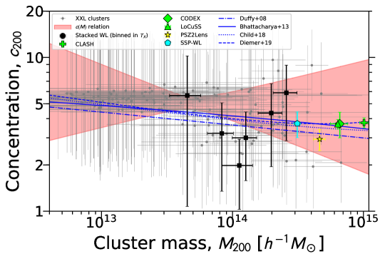
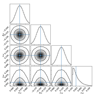
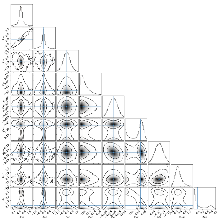
The main results of Bayesian inference for the $c_{200}$–$M_{200}$ relation are summarized in Table 4 and Figure 20. In addition to the regression of the C1+C2 sample, we have also analyzed the C1 subsample separately. Posterior summary statistics ($C_{\mathrm{BI}}\pm S_{\mathrm{BI}}$; see Section 4.1) of for all regression parameters (see Section 5.1.6) are listed in Table 4. Figure 20 shows the marginalized one- and two-dimensional posterior PDFs for the C1+C2 sample.

In Figure 6, we show the resulting $c_{200}$–$M_{200}$ relation at a reference redshift of $z_{\mathrm{ref}}=0.3$ for the C1+C2 sample, along with the theoretical $c_{200}$–$M_{200}$ relations for the full population of DM halos predicted by Duffy et al. (2008), Bhattacharya et al. (2013), Child et al. (2018), and Diemer & Joyce (2019) (see also Diemer & Kravtsov, 2015) (see Section 5.2.2). In Figure 6, we overplot the measured values of ($M_{200},c_{200}$) and their $1\sigma$ uncertainties for individual clusters.

Our inference of the $c_{200}$–$M_{200}$ relation for the C1+C2 sample is summarized as follows (Table 4):

$$c_{200} =\left[4.8\pm 1.0\,(\mathrm{stat})\pm 0.8\,(\mathrm{syst})\right]$$ (40)

$$\times\left(\frac{M_{200}}{10^{14}h^{-1}M_{\odot}}\right)^{-0.07\pm 0.28}\left(\frac{1+z}{1+z_{\mathrm{ref}}}\right)^{-0.03\pm 0.47},$$

with a lognormal intrinsic dispersion at fixed $M_{200}$ of $\sigma(\ln{c_{200}})=\ln{10}\,\sigma_{Y|Z}=(5.3\pm 3.4)\%$, and an upper limit of $<24\%$ at the $99.7\%$ CL. Here we have included a systematic uncertainty of $16\%$ in the normalization of the concentration parameter (Section 4.2 and Appendix A). We find no statistical evidence for redshift evolution of the $c_{200}$–$M_{200}$ relation for the XXL sample: $\gamma_{Y|Z}=-0.03\pm 0.47$.

The $c_{200}$–$M_{200}$ relation inferred for the C1 subsample is highly consistent with that obtained for the full C1+C2 sample (Table 4), indicating that the underlying mass distribution of the XXL cluster population is not sensitive to the details of the X-ray selection function.

The $M_{\mathrm{200,WL}}$–$M_{200}$ relation is found to be poorly constrained given the large statistical uncertainties in our weak-lensing mass estimates. The posterior distribution of $\sigma_{X|Z}$ is bimodal (Figure 20), and there is a distinct lower-scatter solution of $\sigma_{X|Z}\lower 2.15277pt\hbox{$\;\buildrel<\over{\sim}\;$}0.1$ with a tail extending toward the higher-scatter solution. The lower-scatter solution is associated with $\sigma_{Z,0}\sim 0.4$, which is reasonable for the XXL sample (; ). On the other hand, the higher-scatter solution is considerably larger than the theoretically expected level of intrinsic scatter in the weak-lensing mass, $\sim 20\%$ (Becker & Kravtsov, 2011; Gruen et al., 2015). The higher-scatter solution associated with $\ln{10}\sigma_{Z,0}\ll 1$ (see Table 4) is unlikely for the XXL sample (; ).

To assess the impact of this higher-scatter solution on our results, we repeated our regression analysis assuming an informed prior of $\sigma_{X|Z}\sim{\cal U}(0.05,0.15)$ centered at $\sigma_{X|Z}=0.1$, which is approximately the theoretically expected level of intrinsic scatter (Becker & Kravtsov, 2011). With this informed prior, we find $c_{200}=4.9\pm 0.5$ at $M_{200}=10^{14}h^{-1}M_{\odot}$ and $z=0.3$, with $\beta_{Y|Z}=-0.05\pm 0.08$, $\gamma_{Y|Z}=-0.03\pm 0.43$, and $\sigma(\ln{c_{200}})=(5.4\pm 3.5)\%$, which is fully consistent with our baseline results (see Equation (40)). This comparison shows that the higher-scatter solution has negligible impact on the central values of the regression parameters, whereas the size of errors for the normalization and mass slope has been largely decreased, as the parameter space is reduced substantially. On the other hand, we find that the higher-scatter solution has little influence on the central value and uncertainty of $\sigma(\ln{c_{200}})$.

Another source of systematic errors is the choice of the concentration prior in the NFW profile fitting (Section 4.1). Posterior constraints on the NFW parameters for noisy objects, especially on $c_{200}$, are poor and dominated by the priors. We thus tested the sensitivity of our results to the prior chosen for $c_{200}$. We have repeated our NFW fits and regression using an even less informative prior uniform in the range $\log{c_{200}}\in[0,\log{30}]$, obtaining a slightly higher normalization of $c_{200}(z_{\mathrm{ref}})=5.6\pm 1.6$ at $M_{200}=10^{14}h^{-1}M_{\odot}$, $\beta_{Y|Z}=-0.05\pm 0.33$, $\gamma_{Y|Z}=0.03\pm 0.52$, and $\sigma(\ln{c_{200}})=(5.8\pm 3.9)\%$. The changes in the slopes and the intrinsic dispersion are thus negligibly small compared to their respective uncertainties. Hence, the choice of the concentration prior does influence the normalization to some degree, but it does not significantly alter our main results and conclusions even with priors that include unrealistically large concentrations.

5.2.2 Comparison with the Literature

Overall, our regression results are in good agreement with the theoretical predictions from DM-only numerical simulations calibrated for recent $\Lambda$CDM cosmologies (see Figure 6; Bhattacharya et al., 2013; Diemer & Kravtsov, 2015; Klypin et al., 2016; Child et al., 2018; Diemer & Joyce, 2019). In particular, the inferred normalization and mass slope are in good agreement with these DM-only $\Lambda$CDM predictions, which yield mean concentrations in the range $c_{200}(z=0.3)\simeq 3.9$–$4.2$ at $M_{200}=10^{14}h^{-1}M_{\odot}$, with a shallow negative slope of $\beta\simeq-0.09$ (e.g., Child et al., 2018). The inferred intrinsic dispersion $\sigma(\ln{c_{200}})$, however, is significantly smaller than predicted for the full population of $\Lambda$CDM halos, $\sigma(\ln{c_{200}})\simeq 33\%$ (Bhattacharya et al., 2013; Child et al., 2018). We note that our test using simulated weak-lensing observations shows that we can accurately recover the true value of $\sigma(\ln{c_{200}})$ (Figure 14; see Appendix A.2.3). This discrepancy could be due to the X-ray selection bias in terms of the cool-core or relaxation state as found by previous studies (e.g., Buote et al., 2007; Ettori et al., 2010; Eckert et al., 2011; Rasia et al., 2013; Meneghetti et al., 2014; Rossetti et al., 2017). Another possibility is that the statistical errors on $c_{200}$ are overestimated as a consequence of the conservative prior, so that the intrinsic dispersion $\sigma(\ln{c_{200}})$ of the $c_{200}$–$M_{200}$ relation is underestimated.

Although no evidence of redshift evolution for the XXL $c_{200}$–$M_{200}$ relation is found, the average level of concentration for $\Lambda$CDM halos is predicted to decrease with increasing redshift, where the predicted values of the redshift slope range from $\simeq-0.47$ (Duffy et al., 2008), to $-0.42$ (Child et al., 2018), to $-0.29$ (Meneghetti et al., 2014), to $-0.16$ (Ragagnin et al., 2019). Our results are broadly consistent with these predictions within the large statistical uncertainty. We note that the redshift evolution of the concentration parameter is sensitive to the relaxation state of clusters (e.g., De Boni et al., 2013; Meneghetti et al., 2014).

Numerical simulations suggest that relaxed subsamples have concentrations that are on average $\sim 10$% higher than for the full population of halos (Duffy et al., 2008; Bhattacharya et al., 2013; Meneghetti et al., 2014; Child et al., 2018; Ragagnin et al., 2019). This indicates that mean concentrations for relaxed halos are $c_{200}(z=0.3)\simeq 4.3$–$4.6$ at $M_{200}=10^{14}h^{-1}M_{\odot}$, which are consistent with the observational constraint (see Equation (40)). At face value, the $c_{200}$–$M_{200}$ relation obtained for the XXL sample is in better agreement with those predicted for relaxed systems. Another important effect of the relaxation state is that relaxed halos are predicted to have a smaller intrinsic dispersion in the $c_{200}$–$M_{200}$ relation, $\sigma(\ln{c_{200}})\sim 25\%$ (e.g., Neto et al., 2007; Duffy et al., 2008; Bhattacharya et al., 2013), which is again in better agreement with our observational constraint on the XXL sample.

Meneghetti et al. (2014) characterized a sample of halos that closely matches the selection function of the CLASH X-ray-selected subsample with $M_{200}\sim 10^{15}h^{-1}M_{\odot}$ (Donahue et al., 2014; Umetsu et al., 2014, 2016, 2018; Merten et al., 2015). These clusters were selected to have a high degree of regularity in their X-ray morphology (Postman et al., 2012). Cosmological hydrodynamical simulations suggest that this subsample is prevalently composed of relaxed clusters ($\sim 70\%$) and largely free of orientation bias (Meneghetti et al., 2014). Another important effect of the selection function based on X-ray regularity is to reduce the scatter in concentration down to $\sigma(\ln{c_{200}})\sim 16\%$ (see also Rasia et al., 2013). Although the XXL sample was not selected explicitly according to their X-ray morphology, the X-ray selection in favor of relaxed systems is likely to considerably affect the level of scatter in the $c_{200}$–$M_{200}$ relation (Rasia et al., 2013).

In Figure 6, we also compare our results with previously published weak-lensing constraints on X-ray-selected high-mass clusters from the CLASH (Umetsu et al., 2016, $z=0.34$), LoCuSS (Okabe & Smith, 2016, $z=0.23$), and CODEX (Cibirka et al., 2017, $z=0.50$) surveys; PSZ2 clusters detected by the Planck mission (Sereno et al., 2017, $z=0.20$); and weak-lensing-selected clusters from the HSC survey (Miyazaki et al., 2018a, $z=0.27$). Their stacked weak-lensing constraints are in excellent agreement with the DM-only predictions calibrated for recent $\Lambda$CDM cosmologies (e.g., Bhattacharya et al., 2013; Diemer & Kravtsov, 2015; Child et al., 2018; Diemer & Joyce, 2019) and agree with our results. We note that the effect of the redshift evolution is not accounted for in the comparison given in Figure 6.

Biviano et al. (2017) performed a Jeans dynamical analysis of 49 nearby clusters ($0.04\lower 2.15277pt\hbox{$\;\buildrel<\over{\sim}\;$}z\lower 2.15277pt\hbox{$\;\buildrel<\over{\sim}\;$}0.07$) with the projected phase-space distribution of cluster members available from the WINGS and OmegaWINGS survey (Fasano et al., 2006; Gullieuszik et al., 2015). From their dynamical analysis, Biviano et al. (2017) determined total mass density profiles for individual clusters in their sample and derived the $c_{200}$–$M_{200}$ relation over a wide range of cluster mass ($10^{14}\lower 2.15277pt\hbox{$\;\buildrel<\over{\sim}\;$}M_{200}/M_{\odot}\lower 2.15277pt\hbox{$\;\buildrel<\over{\sim}\;$}2\times 10^{15}$). They found a flat $c_{200}$–$M_{200}$ relation, $c_{200}\propto M_{200}^{-0.03\pm 0.09}$, normalized to $c_{200}\simeq 3.8$ at $M_{200}=10^{14}M_{\odot}$, which is in excellent agreement with our results.

5.3. Temperature–Mass Relation

Table 5 Summary Statistics of Regression Parameters for the XXL Temperature–Mass Relation

$\alpha_{Y|Z}$	$\beta_{Y|Z}$	$\gamma_{Y|Z}$	$\sigma_{Y|Z}$	$\alpha_{X|Z}$	$\sigma_{X|Z}$	$\mu_{Z,0}$	$\gamma_{\mu_{Z},D}$	$\sigma_{Z,0}$	$\gamma_{\sigma_{Z},D}$
$0.44\pm 0.09$	$0.85\pm 0.31$	$0.18\pm 0.66$	$0.061\pm 0.049$	$0.00\pm 0.02$	$0.31\pm 0.08$	$-0.17\pm 0.07$	$0.34\pm 0.14$	$0.20\pm 0.07$	$-0.05\pm 0.14$
$0.42\pm 0.07$	$0.75\pm 0.27$	$2/3$	$0.070\pm 0.050$	$-0.00\pm 0.02$	$0.29\pm 0.08$	$-0.17\pm 0.07$	$0.29\pm 0.11$	$0.22\pm 0.06$	$-0.05\pm 0.15$
$0.41\pm 0.05$	$2/3$	$2/3$	$0.070\pm 0.043$	$-0.00\pm 0.02$	$0.29\pm 0.06$	$-0.18\pm 0.07$	$0.34\pm 0.09$	$0.25\pm 0.04$	$-0.04\pm 0.14$

Note. — The $T$–$M$ relation is derived for a subset of 105 clusters that have both measured HSC $M_{500}$ masses and X-ray temperatures $T_{\mathrm{300\,kpc}}$. The intercept $\alpha_{X|Z}$ is a nuisance parameter to marginalize over the residual mass calibration uncertainty of $\pm 5\%$.

Figure 7.— The $T_{\mathrm{X}}$–$M_{500}$ relation for the XXL sample obtained using a subsample of 105 clusters having both XXL temperature and HSC weak-lensing measurements. The gray circles with error bars represent the measured parameters and their $1\sigma$ uncertainties for individual XXL clusters. The red shaded region shows the $1\sigma$ confidence region of the mean $T_{\mathrm{X}}$–$M_{500}$ relation at a reference redshift of $z_{\mathrm{ref}}=0.3$ obtained from our Bayesian regression using the LIRA package. The thick black dashed line shows the XXL DR1 results of XXL Paper IV. Our results are also compared with previously published results for massive clusters obtained by Kettula et al. (2015) and Mantz et al. (2016).

Figure 8.— Same as Figure 7, but with the $E(z)$-trend parameter fixed to the self-similar model expectation of $\gamma_{Y|Z}=2/3$.

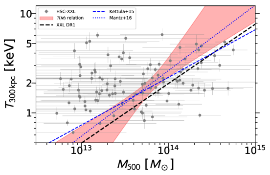
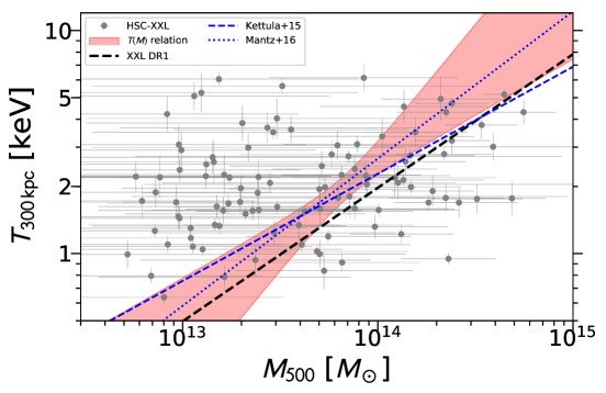
Models of self-similar gravitational collapse in an expanding universe predict scale-free, power-law relations between cluster properties (Kaiser, 1986; Ettori, 2015). Deviations from self-similar behavior are often interpreted as evidence of feedback into the intracluster gas associated with star formation and AGN activities, as well as with radiative cooling in the cluster cores (e.g., Czakon et al., 2015). The self-similar prediction for the $T_{\mathrm{X}}$–$M$ relation is $T_{\mathrm{X}}\propto E^{2/3}(z)M_{\Delta}^{2/3}$, in which the virial condition $GM_{\Delta}/r_{\Delta}\sim T_{\mathrm{X}}$ with $r_{\Delta}\propto[M_{\Delta}/\rho_{\mathrm{c}}(z)]^{1/3}$ is assumed.

On the other hand, secondary infall and continuous accretion from the surrounding large-scale structure can lead to a departure from virial equilibrium (Bertschinger, 1985), while scaling relations of clusters preserve the power-law structure (Fujita et al., 2018b, a). The large scatter in growth histories of clusters translates into a significant diversity in their density profiles (Diemer & Kravtsov, 2014), thus contributing to the scatter of the $T_{\mathrm{X}}$–$M$ relation (Fujita et al., 2018a). The mass dependence of the $c$–$M$ relation and the halo fundamental-plane (FP) relation (Fujita et al., 2018b) make the mass trend of the $T_{\mathrm{X}}$–$M$ relation on cluster scales steeper than the self-similar prediction ($T_{\mathrm{X}}\propto E^{0.75}(z)M_{500}^{0.75}$; Fujita et al., 2018a). However, the mass trend of the $T_{\mathrm{X}}$–$M$ relation is predicted to become shallower and closer to the self-similar expectation toward group scales ($T_{\mathrm{X}}\propto E^{0.65}(z)M_{500}^{0.65}$; Fujita et al., 2018a).

Now we turn to results of Bayesian inference for the $T_{\mathrm{300\,kpc}}$–$M_{500}$ relation. Posterior summary statistics ($C_{\mathrm{BI}}\pm S_{\mathrm{BI}}$; see Section 4.1) for all regression parameters (Section 5.1.6) are listed in Table 5. Figure 21 shows the marginalized one- and two-dimensional posterior PDFs for the regression parameters of the $T_{\mathrm{300\,kpc}}$–$M_{500}$ relation.

Figure 7 shows the resulting $T_{\mathrm{300\,kpc}}$–$M_{500}$ relation for the XXL sample at a reference redshift of $z_{\mathrm{ref}}=0.3$. Our inference of the $T_{\mathrm{300\,kpc}}$–$M_{500}$ relation is summarized as follows:

$$T_{\mathrm{300\,kpc}} =\left(2.78\pm 0.54\right)\,\mathrm{keV}$$ (41)

$$\times\left(\frac{M_{500}}{10^{14}M_{\odot}}\right)^{0.85\pm 0.31}\left[\frac{E(z)}{E(z_{\mathrm{ref}})}\right]^{0.18\pm 0.66},$$

with a lognormal intrinsic dispersion of $\sigma(\ln{T_{\mathrm{300\,kpc}}})=(14\pm 11)\%$ at fixed $M_{500}$. A tighter statistical constraint on the normalization can be obtained around the log-mean mass of clusters inferred for the sample, $\mu_{Z,0}=-0.17\pm 0.07$ at $z_{\mathrm{ref}}=0.3$. The inferred mean mass of the population is $M_{500}=(7.6\pm 1.4)\times 10^{13}M_{\odot}$ at $z_{\mathrm{ref}}=0.3$. For $M_{500}=8\times 10^{13}M_{\odot}$ and $z=0.3$, we find $T_{\mathrm{300\,kpc}}=2.29\pm 0.36\,\mathrm{keV}$.

We find no statistical evidence for redshift evolution of the $T_{\mathrm{300\,kpc}}$–$M_{500}$ relation for the XXL sample: $\gamma_{Y|Z}=0.18\pm 0.66$, which is also consistent with the self-similar expectation, $\gamma_{Y|Z}=2/3$. A slightly shallower mass slope of $\beta_{Y|Z}=0.75\pm 0.27$ is found when performing the regression by setting the $E(z)$-trend parameter to the self-similar expectation, $\gamma_{Y|Z}=2/3$ (see Table 5). The resulting constraints on the $T_{\mathrm{300\,kpc}}$–$M_{500}$ relation are shown in Figure 8. When we fix the slope parameters to $\beta_{Y|Z}=\gamma_{Y|Z}=2/3$ expected from the self-similar model, we find $T_{\mathrm{300\,kpc}}=\left(2.58\pm 0.27\right)\,\mathrm{keV}\times(M_{500}/10^{14}M_{\odot})^{2/3}[E(z)/E(z_{\mathrm{ref}})]^{2/3}$, with a lognormal intrinsic dispersion of $\sigma(\ln{T_{\mathrm{300\,kpc}}})=(16\pm 10)\%$.

Overall, our regression results are in agreement within the errors with the theoretical predictions (Table 5). We find the mass slope parameter $\beta_{Y|Z}$ to be slightly steeper but consistent with the self-similar expectation, $\beta_{Y|Z}=2/3$, as well as with the range $\beta_{Y|Z}\simeq 0.65$–$0.75$ predicted by the halo FP relation of Fujita et al. (2018a). The $E(z)$-trend parameter $\gamma_{Y|Z}$ is still consistent with the self-similar expectation $\gamma_{Y|Z}=2/3$ within the large uncertainty. It should be stressed that we measure the X-ray temperatures $T_{\mathrm{X}}=T_{\mathrm{300\,kpc}}$ in a core-included aperture of 300 kpc (physical), whereas the $r_{500}$ aperture for the XXL sample is typically $\sim 500$–$600$ kpc (physical). Hence, a quantitative interpretation of the observed $T_{\mathrm{300\,kpc}}$–$M_{500}$ relation is not straightforward. For the $M_{500,\mathrm{WL}}$–$M_{500}$ relation, we observe a similar trend of the intrinsic dispersion $\sigma_{X|Z}=\sigma(\ln{M_{500,\mathrm{WL}}})/\ln{10}$ to that in the $c_{200}$–$M_{200}$ relation (Section 5.2).

Recently, Bulbul et al. (2019) studied mass scaling relations of X-ray observables for a sample of 59 SZE-selected high-mass clusters ($3\times 10^{14}M_{\odot}\leqslant M_{500}\leqslant 1.8\times 10^{15}M_{\odot}$, $0.20<z<1.5$) from the South Pole Telescope (SPT) survey. They used SPT SZE-based cluster mass estimates. Since Bulbul et al. (2019) examined the scaling relations with both core-included and core-excised quantities measured from XMM-Newton data (albeit in the high-mass regime), their results are of critical relevance to our study (see Figures 7 and 8). Overall, they found that the mass trends of the X-ray observables are steeper than self-similar behavior in all cases (e.g., $T_{\mathrm{X}}\propto M_{500}^{0.80\pm 0.10}$ including the core region), while the redshift trends are consistent with the self-similar expectation. Their mass and $E(z)$ trends of the $T_{\mathrm{X}}$–$M_{500}$ relation with and without the core region are both consistent with our results (see Table 4 of Bulbul et al., 2019, their fitting results of Form I). According to the findings of Bulbul et al. (2019), the mass and redshift trends, as well as the normalization of the core-included $T_{\mathrm{X}}$–$M_{500}$ relation, are consistent within the errors with those for their core-excised case. The most noticeable difference between the two cases comes from the intrinsic scatter. They found a lognormal intrinsic dispersion of $\sigma(\ln{T_{\mathrm{X}}})=(13\pm 5)\%$ for the core-excised case and $\sigma(\ln{T_{\mathrm{X}}})=(18\pm 4)\%$ for the core-included case. When the core region is included, the intrinsic lognormal dispersion in the $T_{\mathrm{X}}$–$M_{500}$ relation is increased by $\simeq 40\%$, although the difference is not statistically significant.

Our $T_{\mathrm{X}}$–$M_{500}$ relation is in good agreement with that of Mantz et al. (2016) obtained for a sample of 40 dynamically relaxed, X-ray hot ($\lower 2.15277pt\hbox{$\;\buildrel>\over{\sim}\;$}5$ keV) clusters based on Chandra X-ray observations (see Figures 7 and 8). We note that Mantz et al. (2016) used cluster mass estimates obtained from X-ray data assuming hydrostatic equilibrium. They found no significant bias in their X-ray hydrostatic mass estimates relative to weak lensing.

At group scales of $M_{500}\lower 2.15277pt\hbox{$\;\buildrel<\over{\sim}\;$}5\times 10^{13}M_{\odot}$, our regression results agree with the XXL DR1 results of XXL Paper IV based on weak-lensing mass estimates for a subsample of 38 XXL-N clusters at $z<0.6$. Their analysis used the weak-lensing shear catalog from the Canada–France–Hawaii Telescope Lensing Survey (CFHTLenS; Heymans et al., 2012; Erben et al., 2013) to obtain the mass–temperature relation for the XXL sample. Our $T_{\mathrm{300\,kpc}}$–$M_{500}$ relation has a slightly steeper mass trend than the XXL DR1 results, implying a smaller mass scale in the cluster regime. The overall offset from the XXL DR1 relation of XXL Paper IV is at the $\sim 1.5\sigma$ level (Figure 7). When the $E(z)$-trend parameter is fixed to $2/3$, our results are in closer agreement with the XXL DR1 results (Figure 8). In Section 5.4, we provide a detailed comparison of weak-lensing mass estimates between the XXL DR1 and XXL DR2 (this work) results.

Kettula et al. (2015) presented a weak-lensing and X-ray analysis of 12 low-mass clusters selected from the CFHTLenS and XMM-CFHTLS surveys, in combination with high-mass systems from the Canadian Cluster Comparison Project and low-mass systems from the COSMOS survey. Their combined sample comprises 70 systems, spanning more than two orders of magnitude in mass. After correcting for Malmquist and Eddington bias, they found a mass slope of $\beta=0.48\pm 0.06$ in the $T_{\mathrm{X}}$–$M_{500}$ relation with a lognormal intrinsic dispersion of $\sigma(\ln{T_{\mathrm{X}}})=(14\pm 5)\%$. The $T_{\mathrm{X}}$–$M_{500}$ relation of Kettula et al. (2015) is in agreement with our results (see Figures 7 and 8).

5.4. Comparison with the XXL DR1 Mass Calibration

Figure 9.— Comparison of weak-lensing mass estimates for a subset of 23 XXL clusters in common between this work (XXL DR2) and the XXL DR1 results (XXL Paper IV). We characterize the discrepancy between these two sets of weak-lensing mass estimates in the LIRA framework, finding a mean mass offset of $(34\pm 20)\%$ in $M_{\mathrm{500,WL}}$ and $(41\pm 20)\%$ in $M_{\mathrm{200,WL}}$.

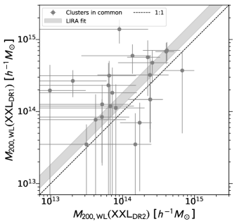
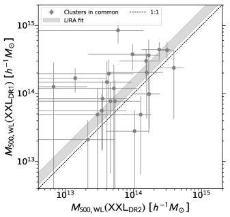
XXL Paper IV derived the mass–temperature ($M_{500}$–$T_{\mathrm{300\,kpc}}$) relation for 38 XXL-N clusters at $z<0.6$ selected from the 100 brightest galaxy cluster (XXL-100-GC) sample (XXL Paper II) by using weak-lensing mass estimates based on the CFHTLenS shear catalog (Heymans et al., 2012; Erben et al., 2013). The CFHTLenS survey covers a total survey area of $\simeq 154$ deg², which overlaps with the XXL-N field. Their shear catalog comprises galaxy shape measurements with an unweighted (weighted) source density of $n_{\mathrm{gal}}\simeq 17$ ($14$) galaxies arcmin^-2, compared to $n_{\mathrm{gal}}\simeq 25$ ($22$) galaxies arcmin^-2 for the HSC survey (see Section 2.2).

Eckert et al. (2016, hereafter XXL Paper XIII) studied the baryon fractions of XXL-100-GC clusters using X-ray gas mass measurements and the weak-lensing-calibrated $M_{500}$–$T_{\mathrm{300\,kpc}}$ relation of XXL Paper IV. They found a low gas mass fraction ($f_{\mathrm{gas,500}}\simeq 0.048$ at $M_{500}=5\times 10^{13}M_{\odot}$) that requires a relative mass bias of $b_{\mathrm{HE}}\equiv 1-M_{\mathrm{500,X}}/M_{\mathrm{500,WL}}=0.28^{+0.07}_{-0.08}$ to match the gas fractions obtained with weak-lensing and X-ray hydrostatic-equilibrium mass estimates, $M_{\mathrm{500,WL}}$ and $M_{500,X}$, respectively.

As summarized below, the shear-to-mass procedure implemented by XXL Paper IV is somewhat different from ours. XXL Paper IV used the same fitting function as in this study (i.e., the projected NFW functional of Wright & Brainerd, 2000), with a similar mass prior that is uniform in the logarithm of $M_{200}$ in the range $\log{(M_{200}/M_{\odot})}\in[13,16]$. The concentration parameter was fixed to the mean $c_{200}$–$M_{200}$ relation of Duffy et al. (2008), which is calibrated for a WMAP 5 yr cosmology (Komatsu et al., 2009). At $M_{200}=10^{14}h^{-1}M_{\odot}$ and $z=0.3$, this model predicts $c_{200}\simeq 3.6$, which is $\simeq 14\%$ lower than predicted by the Bhattacharya et al. (2013) relation, $c_{200}\simeq 4.2$ (see Figure 6). Because of the $c_{200}$–$M_{200}$ degeneracy (see Section 5.4.1 of Umetsu et al., 2014), assuming a lower concentration will result in an overestimation of the total mass, $M_{200}$. By repeating the analysis assuming the fixed $c_{200}$–$M_{200}$ relation of Duffy et al. (2008), we find that the geometric mean mass scale $\langle M_{200}\rangle_{\mathrm{g}}$ of the C1+C2 sample is overestimated by $22\%$ with respect to our fiducial analysis (Table 1).

The fitting radial range chosen by XXL Paper IV is $R\in[0.15,3]$ Mpc (physical), corresponding to $R\in[0.1365,2.73]\,h^{-1}\mathrm{Mpc}$ (comoving) at $z=0.3$. Their fitting range is comparable to our choice $R\in[0.3,3]\,h^{-1}\mathrm{Mpc}$ (comoving), but their fits are more sensitive to the inner region. XXL Paper IV only accounted for the shape noise (see Equation (16)) in their error analysis.

Another possible cause of the mass discrepancy is the choice of posterior summary statistics for the mass scale of each individual cluster (Sereno et al., 2017). XXL Paper IV employed the mode and asymmetric confidence limits of $M_{200}$ as posterior summary statistics. In contrast, we use symmetrized biweight statistics, $C_{\mathrm{BI}}\pm S_{\mathrm{BI}}$. For a lognormally distributed quantity, the biweight center location $C_{\mathrm{BI}}$ typically approximates the median of the distribution. By analyzing simulations of NFW lenses, Sereno et al. (2017) found that the mode estimator is less stable and noisier than the biweight estimator for low-SNR objects (see their Appendix C). For their NFW lenses with $M_{200}>10^{14}h^{-1}M_{\odot}$, Sereno et al. (2017) found that the mode estimator overestimates $M_{200}$ by $4\%$ relative to the biweight estimator, where the actual level of bias depends on the mass range of the sample and the quality of data (Sereno et al., 2017).

It should be emphasized again that XXL Paper IV adopted the quadratic weak-lensing SNR estimator (Equation (15)), which is positive by construction (Section 3.2) and can lead to overestimation of the true significance if the actual SNR per radial bin is less than unity (see Table 2). It is also sensitive to the choice of the number of radial bins (or the number of degrees of freedom).

We have identified 23 XXL clusters in common between the XXL DR1 (XXL Paper IV) and DR2 (this work) mass calibrations, excluding seven clusters for which only upper bounds were obtained by XXL Paper IV. We characterize the discrepancy between the two sets of weak-lensing mass estimates by accounting for the respective scatters with respect to the true mass. To this end, we solve the following coupled, scattered relations in the LIRA framework (Section 5.1):

$$X_{1} =\alpha+Z\pm\sigma_{X_{1}|Z},$$ (42)

$$X_{2} =Z\pm\sigma_{X_{2}|Z},$$

where $Z$ denotes the true logarithmic mass, $X_{1}$ and $X_{2}$ are the logarithmic weak-lensing masses from the XXL DR1 and XXL DR2 mass calibrations, respectively, $\sigma_{X_{1}|Z}$ and $\sigma_{X_{2}|Z}$ are the respective intrinsic dispersions at fixed logarithmic mass $Z$, and $\alpha$ describes the logarithmic mass offset. We simultaneously model the underlying $P(Z)$ characterized by the mean $\mu_{Z,0}$ and the dispersion $\sigma_{Z,0}$ (see Section 5.1). For each cluster, we account for correlations between $X_{1}$ and $X_{2}$ assuming a cross-correlation coefficient of $0.7$ (approximately the ratio of the number densities of source galaxies between the CFHTLenS and HSC shear catalogs).

The results are shown in Figure 9. We find a mean mass offset of $\ln{10}\alpha=(34\pm 20)\%$ in $M_{500}$ and $(41\pm 20)\%$ in $M_{200}$. If we exclude the most discrepant cluster with an XXL DR1 estimate of $M_{\mathrm{200,WL}}\lower 2.15277pt\hbox{$\;\buildrel>\over{\sim}\;$}10^{15}h^{-1}M_{\odot}$, the mass discrepancy is reduced to $(28\pm 18)\%$ in $M_{500}$ and $(35\pm 18)\%$ in $M_{200}$. This is consistent with the level of mass bias found by XXL Paper XIII.

This level of mass discrepancy with respect to DR1 is also comparable to that found by Lieu et al. (2017), who reanalyzed the same CFHT weak-lensing data for the DR1 sample of XXL Paper IV. By fitting $M_{200}$ and $c_{200}$ together in Bayesian hierarchical modeling, Lieu et al. (2017) found weak-lensing $M_{200}$ masses that are on average $\sim 28\%$ smaller (in terms of the weighted geometric mean) than those of XXL Paper IV. This discrepancy is reduced to $\sim 14\%$ when $c_{200}$ is treated as a free parameter in the DR1 analysis of XXL Paper IV (Lieu et al., 2017, see also Section 4.1 of XXL Paper IV).

We thus conclude that the discrepancy between the XXL DR1 and XXL DR2 mass calibrations is likely due to the combination of the fixed $c$–$M$ relation assumed in XXL Paper IV and the different fitting procedures for extracting cluster masses from weak-lensing data.

5.5. Mass Forecasting

Figure 10.— Mass forecasting based on X-ray temperature measurements. The red shaded region shows the $1\sigma$ confidence range of the mean $M_{500}$–$T_{\mathrm{X}}$ relation calibrated with a subsample of 105 XXL clusters having both XXL temperature and HSC weak-lensing measurements (gray circles). The $M_{500}$–$T_{\mathrm{X}}$ relation is obtained by fixing the slopes to the self-similar values. The red circles with error bars show bias-corrected, weak-lensing-calibrated estimates of $M_{500}$ based on $T_{\mathrm{300\,kpc}}$ (Table 2). The black squares with error bars show the stacked weak-lensing constraints obtained for six subsamples of C1+C2 XXL clusters binned in X-ray temperature (see Table 3 and Figure 5). The $M_{500}$–$T_{\mathrm{X}}$ relation from the XXL DR1 results (XXL Paper IV) is shown with the thick black dashed line.

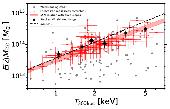
Mass forecasting given a low-scatter mass proxy can be performed in the framework of Bayesian hierarchical modeling (e.g., Sereno, 2016b; Sereno & Ettori, 2017). Here we obtain bias-corrected, weak-lensing-calibrated estimates of $M_{200}$ and $M_{500}$ for individual XXL clusters from their X-ray temperatures by using the LIRA package. To this end, we use the subset of 105 C1+C2 clusters with measured $T_{\mathrm{300\,kpc}}$ values as a calibration sample. In this backward forecasting analysis, we simultaneously model the proxy distribution and determine the $M_{\Delta}$–$T_{\mathrm{300\,kpc}}$ scaling relation (Sereno & Ettori, 2017) for each overdensity $\Delta$.

Figure 10 shows the resulting distribution of weak-lensing-calibrated $M_{500}$ as a function of $T_{\mathrm{300\,kpc}}$ for the calibration sample along with the $M_{500}$–$T_{\mathrm{300\,kpc}}$ relation. Here we considered the scaling relation with the slopes fixed to the self-similar expectation, i.e., $E(z)M_{\Delta}\propto T_{\mathrm{X}}^{3/2}$. In Table 2, we provide cluster mass estimates $M_{\mathrm{200,MT}}$ and $M_{\mathrm{500,MT}}$, where available, based on the $M_{\Delta}$–$T_{\mathrm{300\,kpc}}$ relation. These cluster mass estimates are corrected for statistical bias and selection effects, and the errors of forecasted masses include uncertainties associated with the X-ray temperature measurements, the determination of the scaling relation with the calibration sample, and the intrinsic scatter (Sereno & Ettori, 2017). Additionally, we have included a constant bias correction factor of $1/(1+b_{M_{\Delta}})\simeq 1.1$ to account for mass modeling bias as $M_{\Delta,\mathrm{MT}}\to M_{\Delta,\mathrm{MT}}/(1+b_{M_{\Delta}})$. Here we adopted $b_{M_{\Delta}}\simeq-11\%$ evaluated at $M_{\mathrm{500,true}}=10^{14}M_{\odot}$, the typical mass scale of the XXL sample (see Appendix A.2.2).

The bias-corrected $M_{\Delta}$–$T_{\mathrm{300\,kpc}}$ relation is summarized as

$$E(z)M_{500} =(3.15\pm 0.48)\times 10^{13}M_{\odot}\times\left(\frac{T_{\mathrm{300\,kpc}}}{1\,\mathrm{keV}}\right)^{3/2},$$ (43)

$$E(z)M_{200} =(4.58\pm 0.70)\times 10^{13}M_{\odot}\times\left(\frac{T_{\mathrm{300\,kpc}}}{1\,\mathrm{keV}}\right)^{3/2}.$$

It should be noted that these weak-lensing-calibrated mass estimates are subject to an overall systematic uncertainty of $\pm 5\%$ (Section 4.2). Our results are in good agreement with those of Farahi et al. (2018, hereafter XXL Paper XXIII), who constrained the characteristic mass scale of the XXL sample to be $E(z)M_{200}\simeq 1.3\times 10^{14}M_{\odot}$ at $T_{\mathrm{300\,kpc}}=2$ keV and $z=0.3$ from an ensemble spectroscopic analysis of 132 spectroscopically confirmed C1 and C2 clusters in the XXL-N field.

6. Summary and Conclusions

In this paper, we have presented an ensemble weak-lensing analysis of X-ray galaxy groups and clusters selected from the XXL DR2 catalog (XXL Paper XX) using the HSC survey data (Aihara et al., 2018a; Mandelbaum et al., 2018a). Our joint weak-lensing and X-ray analysis focused on 136 spectroscopically confirmed X-ray-selected systems of class C1 and C2 ($0.031\leqslant z\leqslant 1.033$) detected in the 25 deg² XXL-N region, which largely overlaps with the HSC-XMM field (Figure 1). The area of the overlap region between the two surveys is $21.4$ deg².

With the HSC weak-lensing data, we have measured the tangential shear signal around each individual XXL cluster. We constrained the mass and concentration parameters individually for each cluster by fitting an NFW profile to the $\Delta\Sigma$ profile over the comoving radial range $R\in[0.3,3]\,h^{-1}\mathrm{Mpc}$. In the fitting, we used the covariance matrix $C=C^{\mathrm{shape}}+C^{\mathrm{lss}}+C^{\mathrm{int}}$ that accounts for various sources of statistical errors (Section 3.3). We find an excellent internal consistency between individual and stacked weak-lensing measurements in terms of the weighted average mass of each sample (Table 1; see Equations (24) and (27)). In this consistency check, we find no systematic trend with respect to the X-ray temperature $T_{\mathrm{300\,kpc}}$ (Table 3).

We have characterized the systematic uncertainties in the mass and concentration measurements using both empirical approaches and simulations (Section 4.2). There are two possible main sources of systematics in our weak-lensing analysis of the XXL sample: (i) modeling of systems detected with low values of weak-lensing SNR (Figure 3) and (ii) the modeling uncertainty due to systematic deviations from the assumed NFW form in projection. We used two complementary sets of simulations to assess the impact of these systematic effects (Appendix A).

To examine the first possibility, we analyzed synthetic weak-lensing data based on simulations of analytical NFW lenses (Appendix A.1), which closely match our observations in terms of the weak-lensing SNR distribution (Figures 11 and 12). Simulations show that the overall mass scale of an XXL-like sample can be recovered within $3.3\%$ accuracy from individual cluster mass estimates, with no systematic dependence on cluster mass $M_{\mathrm{true}}$. This level of systematic uncertainty is below the statistical precision of the current full sample, $\simeq 9\%$ at $M_{200}\sim 9\times 10^{13}h^{-1}M_{\odot}$ (Table 1). Our shear-to-mass procedure is also stable and unbiased against the presence of low-SNR clusters (Figure 13).

On the other hand, the results from the DM-only BAHAMAS simulation suggest a significant level of mass bias of $\sim-20\%$ for low-mass group systems with $M_{\mathrm{200,true}}\lower 2.15277pt\hbox{$\;\buildrel<\over{\sim}\;$}4\times 10^{13}h^{-1}M_{\odot}$ (Appendix A.2; see Table 6). Since we do not find such a mass-dependent behavior when using the correct mass profile shape (Appendix A.1), this negative bias is likely caused by systematic deviations from the assumed NFW profile shape in projection (Section 4.1). With the present data, the typical mass measurement uncertainty for such low-mass groups is $\sigma(M)/M\sim 140\%$ per cluster. Even when averaging over all such clusters, the statistical uncertainty on the mean mass is of the order of $\lower 2.15277pt\hbox{$\;\buildrel>\over{\sim}\;$}20\%$ (Section 4.3). Therefore, this level of systematic bias ($\lower 2.15277pt\hbox{$\;\buildrel<\over{\sim}\;$}1\sigma$) is not expected to significantly affect the present analysis. In principle, one can correct for such mass-dependent calibration bias using a Bayesian regression approach to forward-modeling such systematic effects.

We have established the $c_{200}$–$M_{200}$ relation for the full C1+C2 sample of 136 XXL clusters, by accounting for selection bias and statistical effects and marginalizing over the overall mass calibration uncertainty of $5\%$ (Section 5.2). We find the mass slope of the $c_{200}$–$M_{200}$ relation to be $\beta_{Y|Z}=-0.07\pm 0.28$ and the normalization to be $c_{200}=4.8\pm 1.0\,(\mathrm{stat})\pm 0.8\,(\mathrm{syst})$ at $M_{200}=10^{14}h^{-1}M_{\odot}$ and $z=0.3$ (Table 4 and Figure 20).

As shown in Figure 6, our weak-lensing results on the $c_{200}$–$M_{200}$ relation are in good agreement with those found for X-ray, SZE, and weak-lensing-selected high-mass clusters (Umetsu et al., 2016; Okabe & Smith, 2016; Cibirka et al., 2017; Sereno et al., 2017; Miyazaki et al., 2018a), as well as with DM-only predictions calibrated for recent $\Lambda$CDM cosmologies (e.g., Bhattacharya et al., 2013; Diemer & Kravtsov, 2015; Child et al., 2018; Diemer & Joyce, 2019). Our results are also in excellent agreement with the $c_{200}$–$M_{200}$ relation obtained by Biviano et al. (2017) for a sample of 49 nearby clusters from a dynamical analysis of the projected phase-space distribution of cluster members.

The lognormal intrinsic dispersion in the $c_{200}$–$M_{200}$ relation for the XXL sample is constrained as $\sigma(\ln{c_{200}})<24\%$ ($99.7\%$ CL), which is smaller than predicted for the full population of $\Lambda$CDM halos, $\sigma(\ln{c_{200}})\sim 33\%$ (Bhattacharya et al., 2013; Child et al., 2018). This discrepancy is likely caused in part by the X-ray selection bias in terms of the cool-core or relaxation state (e.g., Buote et al., 2007; Ettori et al., 2010; Rasia et al., 2013). Alternatively, the intrinsic dispersion $\sigma(\ln{c_{200}})$ can be underestimated if the statistical errors on $c_{200}$ for individual clusters are overestimated.

We have also determined the $T_{\mathrm{X}}$–$M_{500}$ relation for a subset of 105 XXL clusters that have both measured HSC lensing masses, $M_{500}$, and X-ray temperatures, $T_{\mathrm{300\,kpc}}$ (Section 5.3; see Table 5 and Figure 21). Again, we have accounted for selection bias and statistical effects, marginalizing over the mass calibration uncertainty of $5\%$. We find the mass slope of the $T_{\mathrm{X}}$–$M_{500}$ relation to be $\beta_{Y|Z}=0.85\pm 0.31$ and the normalization to be $T_{\mathrm{300\,kpc}}=2.78\pm 0.54$ keV at $M_{500}=10^{14}M_{\odot}$ and $z=0.3$, with a lognormal intrinsic dispersion of $\sigma(\ln{T_{\mathrm{300\,kpc}}})=(14\pm 11)\%$.

The resulting $T_{\mathrm{X}}$–$M_{500}$ relation is consistent within the errors with the secondary-infall prediction based on the halo FP relation (Fujita et al., 2018b, a), as well as with the self-similar expectation. Our $T_{\mathrm{X}}$–$M_{500}$ relation is also in agreement with those obtained by Kettula et al. (2015) and Mantz et al. (2016) (Figures 7 and 8). At group scales, our results agree with the XXL DR1 results of XXL Paper IV based on the CFHTLenS shear catalog (Figure 7). However, our $T_{\mathrm{X}}$–$M_{500}$ relation has a slightly steeper mass trend, implying a smaller mass scale in the cluster regime. The overall offset in the $T_{\mathrm{X}}$–$M_{500}$ relation is at the $\sim 1.5\sigma$ level (Figures 7 and 8), corresponding to a mean mass offset of $(34\pm 20)\%$ (Section 5.4; see Figure 9). This discrepancy is likely due to the different fitting procedures for extracting cluster masses from weak-lensing data (Section 5.4; see also Lieu et al., 2017).

The change of the mass scale has important implications for cluster astrophysics probed with the XXL sample. Compared to the XXL DR1 results (XXL Paper IV), our HSC mass calibration leads to a higher gas mass fraction, $f_{\mathrm{gas,500}}=0.053\pm 0.015$ at $M_{500}=5\times 10^{13}M_{\odot}$ and $z=0.3$, and a lower level of hydrostatic mass bias, $b_{\mathrm{HE}}=(9\pm 17)\%$ (Sereno et al., 2020). Our HSC weak-lensing analysis thus alleviates the tension reported by XXL Paper XIII. On the other hand, this slight decrease of the mass scale has a direct impact on the cosmological interpretation of the abundance (Pacaud et al., 2018, hereafter XXL Paper XXV) and clustering properties (Marulli et al., 2018, hereafter XXL Paper XVI) of the XXL sample across cosmic time.

Finally, we have produced bias-corrected, weak-lensing-calibrated mass estimates, $M_{\mathrm{200,MT}}$ and $M_{\mathrm{500,MT}}$, for individual XXL clusters based on their X-ray temperatures (Section 5.5; see Table 2). We recommend using these statistically corrected $M_{\Delta,\mathrm{MT}}$ as a mass estimate for a given individual cluster. It is important to note that the weak-lensing-calibrated $M_{\Delta}$–$T_{\mathrm{X}}$ relation (Equation (43)) allows us to estimate $M_{200}$ and $M_{500}$ for all XXL clusters with measured X-ray temperatures, including those in the XXL-S region. Such lensing-calibrated mass estimates corrected for statistical and selection effects will be particularly useful for a statistical characterization of cluster properties through multiwavelength follow-up observations.

Appendix A Mass Measurement Tests

Figure 11.— Synthetic weak-lensing observations from simulations of 1000 NFW lenses at $z=0.3$. Left panel: histogram distribution of the weak-lensing SNR derived from synthetic weak-lensing data. Right panel: histogram distribution of the true cluster mass $M_{\mathrm{200,true}}$. The histograms are shown separately for subsamples of weak-lensing $\mathrm{SNR}<0$ (red shaded) and $\mathrm{SNR}<1$ (gray shaded), as well as for the full sample (blue).

Figure 12.— Left panel: comparison of the weak-lensing SNR and the true mass $M_{\mathrm{200,true}}$ (gray circles) for a synthetic sample of 1000 NFW lenses (see Figure 11). The red solid and red dashed horizontal lines represent $\mathrm{SNR}=1$ and $\mathrm{SNR}=0$, respectively. Middle panel: weak-lensing SNR versus weak-lensing mass $M_{\mathrm{200,WL}}$ estimated from the synthetic weak-lensing data using the same analysis pipeline as for the real observations. The blue squares represent weighted geometric means in six logarithmic $M_{200}$ bins, where the vertical bars show the standard deviation of the weak-lensing SNR and the horizontal bars show the full width of each mass bin. Right panel: same as the middle panel, but for the real observations of the XXL sample. The gray circles and red crosses represent the C1 and C2 subsamples, respectively.

Figure 13.— Comparison of the true and estimated values of the mass and concentration parameters $M_{500}$ (left), $M_{200}$ (middle), and $c_{200}$ (right) from synthetic weak-lensing observations of 1000 NFW lenses at $z=0.3$ (see Figure 12). In each panel, the error-weighted geometric mean ratio of the simulated sample, $\langle M_{\Delta,\mathrm{WL}}/M_{\Delta,\mathrm{true}}\rangle_{\mathrm{g}}$ or $\langle c_{\mathrm{200,WL}}/c_{\mathrm{200,true}}\rangle_{\mathrm{g}}$, is marked with a solid line. Similarly, the shaded blue boxes represent weighted geometric mean ratios and their errors in four equally log-spaced $M_{\mathrm{true}}$ bins. The weighted average mass ratio $\langle M_{\Delta,\mathrm{WL}}/M_{\Delta,\mathrm{true}}\rangle_{\mathrm{g}}$ is consistent with unity to better than $2\sigma$ in all mass bins. Overall, $c_{\mathrm{200,WL}}$ is biased high at a mean level of $(13\pm 3)\%$, with no evidence of systematic mass dependence.

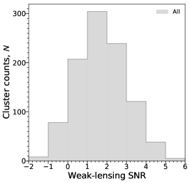
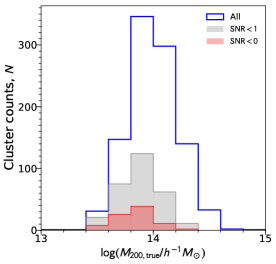
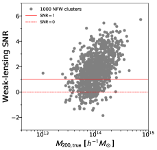
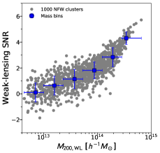
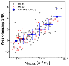
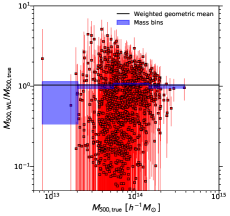
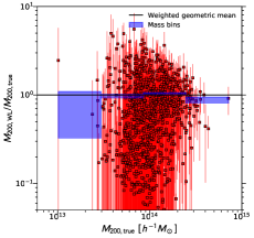
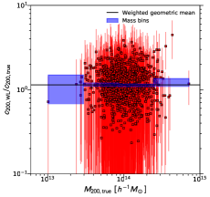
A.1. Simulations of Analytical NFW Lenses

First, we test and quantify the accuracy of our cluster mass measurements using synthetic weak-lensing data that closely match the HSC survey in terms of the weak-lensing SNR distribution. Specifically, the aim of this test is to assess the impact of low weak-lensing SNR objects on ensemble mass measurements for a sample of XXL-like clusters. To this end, we create synthetic weak-lensing data from simulations of analytical NFW lenses at a redshift of $z=0.3$, the median redshift of the full C1+C2 sample (Table 1). We model the weak-lensing signal of each cluster using the “true” profile shape (i.e., NFW), with $M_{200}$ and $c_{200}$ as fitting parameters. We use the same analysis pipeline as done for the real observations. In this way, we can separate possible sources of systematic effects. Hence, any significant level of mass bias, especially in the low-mass regime, would indicate systematics effects caused by noisy mass estimates for low-SNR objects.

A synthetic sample of 1000 NFW lenses was drawn from a Gaussian intrinsic PDF in $Z=\log{(M_{200}/h^{-1}M_{\odot})}$ with a mean $\mu_{Z}=\langle Z\rangle=14$ and a dispersion $\sigma_{Z}=0.5/\ln{10}$, which closely resembles the XXL cluster sample (; ). Concentrations were drawn from the scattered $c_{200}$–$M_{200}$ relation of Bhattacharya et al. (2013) with a lognormal intrinsic dispersion of $\sigma(\ln{c_{200}})=0.15\ln{10}\simeq 35\%$. The range of true $M_{200}$ masses for the simulated sample is $1.0\times 10^{13}\lower 2.15277pt\hbox{$\;\buildrel<\over{\sim}\;$}M_{200}/(h^{-1}M_{\odot})\lower 2.15277pt\hbox{$\;\buildrel<\over{\sim}\;$}7.2\times 10^{14}$ (see the right panel of Figure 11). The synthetic data include the cosmic noise contribution due to the projected uncorrelated large-scale structure, as well as the random shape noise, with a net intrinsic shear dispersion of $\sigma_{g}=0.4$ per shear component. Source galaxies are distributed over the redshift range $0.3<z_{s}<1.2$ with a mean number density of $n_{\mathrm{gal}}=17$ galaxies arcmin^-2. Finally, the $\Delta\Sigma(R)$ profiles were simulated in eight equally spaced logarithmic bins of comoving cluster radius ($R$) from $R_{\mathrm{min}}=0.3h^{-1}\mathrm{Mpc}$ to $R_{\mathrm{max}}=3h^{-1}\mathrm{Mpc}$, to be consistent with the observations (Section 3.2).

The left panel of Figure 11 shows the distribution of weak-lensing SNR measured in a fixed comoving aperture of $R\in[0.3,3]\,h^{-1}\mathrm{Mpc}$ for 1000 simulated NFW lenses. The values of weak-lensing SNR span the range from $-1.9$ to $5.7$, with a median of $1.7$ and a standard deviation of $1.3$, closely mimicking the observed SNR distribution (Figure 3). About $30\%$ ($9\%$) of simulated NFW lenses are detected with weak-lensing $\mathrm{SNR}<1$ (0), as shown in the right panel of Figure 11). The left (middle) panel of Figure 12 compares the weak-lensing SNR and $M_{\mathrm{200,true}}$ ($M_{\mathrm{200,WL}}$) for all NFW lenses in the sample. The resulting distribution of simulated NFW lenses in the SNR–$M_{\mathrm{200,WL}}$ plane reproduces the observations of the XXL sample fairly well (see the right panel of Figure 12).

The weighted average weak-lensing mass $\langle M_{\mathrm{200,WL}}\rangle_{\mathrm{g}}=(1.28\pm 0.03)\times 10^{14}h^{-1}M_{\odot}$ over the full sample (in terms of the error-weighted geometric mean; see Equation 24) is $\simeq 30\%$ higher than the true log-mean (or the true median) mass, $M_{\mathrm{200,true}}=10^{14}h^{-1}M_{\odot}$, and the true mean mass of the population, $M_{\mathrm{200,true}}\simeq 1.13\times 10^{14}h^{-1}M_{\odot}$. Qualitatively, this is because the weighted geometric mean estimator assigns higher weights to those objects with smaller measurement errors, which are likely to be more massive objects. The degree to which $\langle M_{\mathrm{200,WL}}\rangle_{\mathrm{g}}$ is different from the true population mean should depend on both the shape of the intrinsic mass PDF and the level of observational noise.

We introduce the following quantity to characterize the level of bias in the average cluster mass estimated from weak lensing:

$$1+b_{\mathrm{sim},M_{\Delta}}=\langle M_{\Delta,\mathrm{WL}}/M_{\Delta,\mathrm{true}}\rangle_{\mathrm{g}},$$ (A1)

where $M_{\Delta,\mathrm{true}}$ represents the true $M_{\Delta}$ mass from simulations and $M_{\Delta,\mathrm{WL}}$ represents the $M_{\Delta}$ mass estimated from weak lensing. Similarly, we define the bias parameter $b_{\mathrm{sim},c_{200}}$ for the concentration parameter, $c_{200}$.

Figure 13 shows that $b_{\mathrm{sim},M_{500}}$ and $b_{\mathrm{sim},M_{200}}$ are consistent with zero to better than $2\sigma$ in all mass bins, with no significant mass dependence over the full range of $M_{\Delta,\mathrm{true}}$. On the other hand, $c_{\mathrm{200,WL}}$ is biased high at a mean level of $b_{\mathrm{sim},c_{200}}=(13\pm 3)\%$, with no evidence of systematic mass dependence. This systematic offset is likely because the typical scale radius for this sample ($r_{\mathrm{s}}\simeq 0.21\,h^{-1}\mathrm{Mpc}$ in comoving length units) lies below the radial range for fitting, $R\in[0.3,3]\,h^{-1}\mathrm{Mpc}$ (comoving).

In this realization, there are a total of 86 clusters with negative values of weak-lensing SNR. Their weak-lensing mass estimates span the range $M_{\mathrm{200,WL}}\in[0.4,11]\times 10^{13}h^{-1}M_{\odot}$, with a median value of $1.0\times 10^{13}h^{-1}M_{\odot}$, which is comparable to our observations (Section 4.3). The median mass uncertainty of these clusters is $S_{\mathrm{BI}}(M_{\mathrm{200,WL}})/C_{\mathrm{BI}}(M_{\mathrm{200,WL}})\sim 140\%$. This indicates that such noisy objects can reach $M_{\mathrm{200,WL}}/M_{\mathrm{200,true}}\sim 4$ (i.e., the boundary of the $99.7\%$ confidence region; see Figure 13). As shown in the right panel of Figure 11 (see also the left panel of Figure 12), these clusters span a fairly representative range in “true” mass: $M_{200}\in[2.7,19]\times 10^{13}h^{-1}M_{\odot}$, with a median value of $7.0\times 10^{13}h^{-1}M_{\odot}$ and a mean value of $7.5\times 10^{13}h^{-1}M_{\odot}$. At a given true mass, it is expected that there is a statistical counterpart of positively scattered clusters with apparently boosted SNR and thus overestimated $M_{\Delta,\mathrm{WL}}$. In fact, we do not find any significant bias in ensemble weak-lensing mass measurements even at low-mass scales (Figure 13). In contrast, if one selects a subsample of clusters according to their weak-lensing SNR values or mass estimates, they are no more representative of the parent population. In particular, such an SNR-limited selection will bias high the weak-lensing mass estimates at a given X-ray cut, an effect known as the Malmquist bias (e.g., Sereno et al., 2015a; Sereno & Ettori, 2017; Sereno et al., 2017).

A.2. BAHAMAS Simulation

A.2.1 Simulated Halos and Synthetic Weak-lensing Data

Figure 14.— Halo mass and concentration of 639 $\Lambda$CDM halos (gray circles) selected from a DM-only realization of BAHAMAS simulations at $z=0.25$. The thick black line shows the $c_{200}$–$M_{200}$ relation of the selected sample. The lognormal intrinsic scatter ($1\sigma$) around this relation is indicated by a pair of black dashed lines. The red shaded region shows the $1\sigma$ range of the mean $c_{200}$–$M_{200}$ relation recovered from a regression analysis of the synthetic weak-lensing measurements $(M_{\mathrm{200,WL}},c_{\mathrm{200,WL}})$ shown in Figure 17. Here an upward correction of $16\%$ is applied to the normalization inferred from the regression analysis. The inferred intrinsic scatter ($1\sigma$) is indicated by a pair of red dashed lines.

Figure 15.— Synthetic weak-lensing observations from a DM-only realization of BAHAMAS simulations at $z=0.25$. Left panel: histogram distribution of the weak-lensing SNR derived from synthetic weak-lensing data. The black dashed histogram shows an XXL-weighted distribution of the sample. Right panel: histogram distribution of the true cluster mass $M_{\mathrm{500,true}}$. The histograms are shown for subsamples of weak-lensing $\mathrm{SNR}<1$ (gray shaded) and $\mathrm{SNR}<0$ (red shaded), as well as for the full sample (blue solid). The blue dashed histogram shows an XXL-weighted distribution of the sample.

Figure 16.— Left panel: comparison of the weak-lensing SNR and the true mass $M_{\mathrm{200,true}}$ (gray circles) for a sample of 639 $\Lambda$CDM halos selected from a DM-only realization of BAHAMAS simulations. The red solid and red dashed horizontal lines represent $\mathrm{SNR}=1$ and $\mathrm{SNR}=0$, respectively. Right panel: weak-lensing SNR versus total mass $M_{\mathrm{200,WL}}$ (gray circles) estimated from synthetic weak-lensing using the same analysis pipeline as done for the real observations (see Figure 12). The blue squares represent weighted geometric means in nine logarithmic $M_{200}$ bins, where the vertical bars show the standard deviation of the weak-lensing SNR and the horizontal bars show the full width of each mass bin.

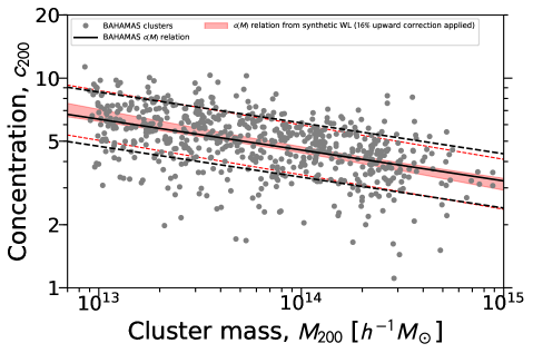
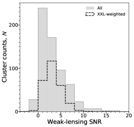
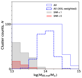
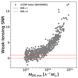
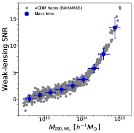
Next, we test and characterize the accuracy of our weak-lensing mass measurements using synthetic observations of realistic $\Lambda$CDM halos, selected from a DM-only run from the BAHAMAS simulations (McCarthy et al., 2017, 2018). The aim of this test is to assess the impact of modeling uncertainties in the projected cluster profile shape down to low-mass group scales. The specific simulation we use adopts a flat $\Lambda$CDM cosmology with WMAP 9 yr cosmological parameters in a box of 400$\,h^{-1}\mathrm{Mpc}$ (comoving) on a side with $1024^{3}$ particles. The particle mass is $3.85\times 10^{9}h^{-1}M_{\odot}$ and the softening length is $4h^{-1}\mathrm{kpc}$ (physical).

To efficiently survey any mass-dependent bias in our methodology, we randomly select 100 halos per logarithmic mass bin $\Delta\log{M_{500}}=0.25$ over the mass range $\log{(M_{500}/M_{\odot})}\in[13,15]$ from the simulation (i.e., a total of eight logarithmic mass bins), at a redshift of $z=0.25$. We note that given the finite size of the simulation volume, the two highest-mass bins have fewer than 100 unique halos (they have 32 and 7, respectively). For these bins, we select all halos for analysis, yielding a total sample of 639 halos.

Figure 14 shows the distribution of selected halos in the $c_{200}$–$M_{200}$ plane. The $c_{200}$–$M_{200}$ relation of the selected sample is described by a power law of the form $c_{200}=4.5\times(M_{200}/10^{14}h^{-1}M_{\odot})^{-0.15}$ with a lognormal intrinsic dispersion of $\sigma(\ln{c_{200}})=30\%$. The right panel of Figure 15 shows the distribution of the selected halos in $M_{\mathrm{500,true}}$ (blue solid histogram), along with an XXL-weighted distribution (blue dashed histogram) where the counts are weighted by the mass PDF expected for the XXL sample (Appendix A.1).

Around each selected halo, we extract all particles in a cube of length 30 Mpc (physical) centered on the most bound particle of each selected halo. The particle distribution is then projected along the $z$-axis and interpolated to a regular two-dimensional grid using a triangular-shaped cloud algorithm to produce an image of surface mass density. We compute convergence and reduced shear maps from the surface mass density map following the methods described in McCarthy et al. (2018, see their Section 3.4.3), assuming a single source redshift plane at $z_{s}=0.829$. We randomly sample the reduced shear maps to obtain a mean background source density of $n_{\mathrm{gal}}=20$ galaxies arcmin^-2. We then add shape noise to the selected shear values, drawing from a normal distribution with a dispersion of $\sigma_{g}=0.28/\sqrt{2}\simeq 0.20$ per shear component.

A.2.2 NFW Modeling

Table 6 Systematic Bias in Weak-lensing Mass Modeling

				NFW Model			Halo Model
$M_{\mathrm{500,true}}$	$M_{\mathrm{200,true}}$	$c_{\mathrm{200,true}}$	$N_{\mathrm{cl}}$	$b_{\mathrm{sim},M_{500}}$	$b_{\mathrm{sim},M_{200}}$	$b_{\mathrm{sim},c_{200}}$	$b_{\mathrm{sim},M_{500}}$	$b_{\mathrm{sim},M_{200}}$	$b_{\mathrm{sim},c_{200}}$
($10^{13}h^{-1}M_{\odot}$)	($10^{13}h^{-1}M_{\odot}$)			($\%$)	($\%$)	($\%$)	($\%$)	($\%$)	($\%$)
$0.8$	$1.2$	$6.1$	$100$	$-19\pm 8$	$-15\pm 8$	$-14\pm 8$	$-15\pm 8$	$-12\pm 9$	$-13\pm 8$
$1.5$	$2.2$	$5.7$	$100$	$-24\pm 7$	$-22\pm 7$	$-18\pm 7$	$-20\pm 7$	$-19\pm 7$	$-16\pm 8$
$2.8$	$3.9$	$5.6$	$100$	$-21\pm 6$	$-18\pm 6$	$-13\pm 8$	$-16\pm 6$	$-14\pm 6$	$-10\pm 8$
$4.9$	$7.4$	$5.0$	$100$	$-11\pm 5$	$-9\pm 5$	$-24\pm 6$	$-7\pm 5$	$-5\pm 5$	$-24\pm 6$
$8.8$	$12.4$	$4.6$	$100$	$-5\pm 3$	$-2\pm 3$	$-28\pm 4$	$-2\pm 3$	$2\pm 3$	$-30\pm 4$
$15.8$	$23.1$	$4.1$	$100$	$8\pm 2$	$8\pm 2$	$-13\pm 4$	$10\pm 2$	$11\pm 3$	$-16\pm 4$
$25.5$	$37.0$	$4.0$	$32$	$3\pm 3$	$6\pm 3$	$-24\pm 5$	$4\pm 3$	$8\pm 4$	$-26\pm 5$
$55.5$	$74.5$	$3.2$	$7$	$1\pm 4$	$9\pm 6$	$-2\pm 8$	$2\pm 4$	$10\pm 5$	$-3\pm 8$

Note. — We characterize the accuracy of our weak-lensing mass measurements using synthetic observations of 639 $\Lambda$CDM halos at $z=0.25$ selected from a DM-only realization of BAHAMAS simulations. We quantify the level of bias in the average cluster mass from weak lensing as $1+b_{\mathrm{sim},M_{\Delta}}(M_{\Delta,\mathrm{true}})=\langle M_{\Delta,\mathrm{WL}}/M_{\Delta,\mathrm{true}}\rangle_{\mathrm{g}}$, where $M_{\Delta,\mathrm{true}}$ is the true $M_{\Delta}$ mass, $M_{\Delta,\mathrm{WL}}$ is the $M_{\Delta}$ mass estimated from weak lensing, and those quantities in brackets with subscript ”g”e denote error-weighted geometric means (Equation (24)). Similarly, we define the bias parameter $b_{\mathrm{sim},c_{200}}$ for the concentration parameter.

Figure 17.— Comparison of the true and estimated values of $M_{500}$ (left), $M_{200}$ (middle), and $c_{200}$ (right) from synthetic weak-lensing observations of 639 $\Lambda$CDM halos at $z=0.25$ selected from a DM-only realization of BAHAMAS simulations. We model the weak-lensing signal of each individual cluster assuming an NFW profile. In each panel, the weighted geometric mean ratio of the simulated sample, $\langle M_{\Delta,\mathrm{WL}}/M_{\Delta,\mathrm{true}}\rangle_{\mathrm{g}}$ or $\langle c_{\mathrm{200,WL}}/c_{200,\mathrm{true}}\rangle_{\mathrm{g}}$, is marked with a solid line. Similarly, the shaded blue boxes represent weighted geometric mean ratios and their errors in eight equally log-spaced $M_{\mathrm{true}}$ bins.

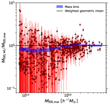
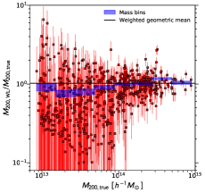
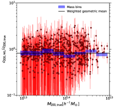
We analyze the synthetic weak-lensing data using the same analysis pipeline as for the real observations (Section 3). We compute for each cluster halo the synthetic $\Delta\Sigma_{+}$ profile (Equation (4)) and model the weak-lensing signal assuming a spherical NFW profile with $M_{200}$ and $c_{200}$ as fitting parameters, following the procedures laid down in Section 4.

The left panel of Figure 15 shows the distribution of weak-lensing SNR measured in a fixed comoving aperture of $R\in[0.3,3]\,h^{-1}\mathrm{Mpc}$ for our sample of 639 halos. The values of weak-lensing SNR span the range from $-2.1$ to $17$, with a median of $2.5$ and a standard deviation of $2.9$. About $20\%$ ($5\%$) of simulated halos are detected with weak-lensing $\mathrm{SNR}<1$ ($0$), as shown in the right panel of Figure 15. The left (right) panel of Figure 16 compares the weak-lensing SNR and $M_{\mathrm{200,true}}$ ($M_{\mathrm{200,WL}}$) for all halos in the BAHAMAS sample. The shape noise level assumed in this set of synthetic data is about a factor of $2$ smaller than that in the NFW-based simulations (Appendix A.1).

In Figure 17, we compare the true and estimated values of ($M_{500},M_{200},c_{200}$) for our simulated sample of 639 halos. For each quantity, we compute the weighted geometric mean ratio between the estimated and true values over the full sample, finding $b_{\mathrm{sim},M_{500}}=(0.9\pm 1.3)\%$, $b_{\mathrm{sim},M_{200}}=(2.1\pm 1.5)\%$, and $b_{\mathrm{sim},c_{200}}=(-18\pm 2)\%$.

We also quantify the levels of bias in the average weak-lensing mass and concentration as a function of $M_{\mathrm{true}}$. Table 6 lists the values of bias in our weak-lensing measurements of ($M_{500},M_{200},c_{200}$) estimated in eight equally log-spaced $M_{500}$ bins (see Figure 15). We find a significant level of mass bias of $\sim-20\%$ for low-mass group halos with $M_{\mathrm{200,true}}\lower 2.15277pt\hbox{$\;\buildrel<\over{\sim}\;$}4\times 10^{13}h^{-1}M_{\odot}$, or $M_{\mathrm{500,true}}\lower 2.15277pt\hbox{$\;\buildrel<\over{\sim}\;$}3\times 10^{13}h^{-1}M_{\odot}$. However, such a low-mass population is expected to be subdominant in the XXL sample (Figures 10 and 15). At the typical mass scale $M_{500}\simeq 7\times 10^{13}h^{-1}M_{\odot}=10^{14}M_{\odot}$ of the XXL sample, we find the level of bias in $M_{\mathrm{200,WL}}$ and $M_{\mathrm{500,WL}}$ to be $\simeq-11\%$.

A.2.3 Recovery of the $c$–$M$ Relation

Here we test how well the parameters describing the $c_{200}$–$M_{200}$ relation can be recovered from cluster weak-lensing observations. To this end, we perform a LIRA regression analysis of our synthetic weak-lensing measurements $(M_{\mathrm{200,WL}},c_{\mathrm{200,WL}})$ for the BAHAMAS sample. We adopt slightly different priors to model the BAHAMAS sample in the LIRA framework (Section 5.1). First, we set $\gamma_{Y|Z}=\gamma_{\mu_{Z},{\cal D}}=\gamma_{\sigma_{Z},{\cal D}}=0$ because all halos are sampled at a single redshift of $z=0.25$. Next, we need $\sigma_{Z,0}\lower 2.15277pt\hbox{$\;\buildrel>\over{\sim}\;$}1$ to approximate $P(Z)$ of the BAHAMAS sample (see Figure 15) with a lognormal distribution in $Z=\log{(M_{200}/10^{14}h^{-1}M_{\odot})}$. Since such a solution is strongly disfavored by the assumed prior for $\sigma_{Z,0}$ (see Equation (39)), we fix the center and width of the lognormal mass PDF to $\mu_{Z,0}=0$ and $\sigma_{Z,0}=1$, respectively. We thus have a total of four regression parameters, ($\alpha_{Y|Z},\beta_{Y|Z},\sigma_{Y|Z},\sigma_{X|Z}$).

The results are shown in Figures 14 and 19. The $c_{200}$–$M_{200}$ relation recovered from the synthetic data is summarized as $c_{200}=(3.7\pm 0.1)\times(M_{200}/10^{14}h^{-1}M_{\odot})^{-0.14\pm 0.02}$ with a logarithmic intrinsic dispersion of $\sigma(\ln{c_{200}})=\ln{10}\sigma_{Y|Z}=(27\pm 3)\%$. We thus accurately recover the true input values of $\beta_{Y|Z}=0.15$ and $\sigma(\ln{c_{200}})=30\%$ (see Appendix A.2.1) within the statistical uncertainties. On the other hand, we underestimate the normalization of the $c_{200}$–$M_{200}$ relation by $(18\pm 2)\%$, as found in Appendix A.2.2. The intrinsic dispersion of the $M_{\mathrm{200,WL}}$–$M_{200}$ relation is found to be $\sigma(\ln{M_{\mathrm{200,WL}}})=\ln{10}\sigma_{X|Z}=(6.5\pm 4.8)\%$, with an upper limit of $<23\%$ ($33\%$) at the $95\%$ ($99.7\%$) CL (see Figure 19). In Figure 14, we have applied an upward correction of $16\%$ to the normalization inferred from the regression analysis.

As a sanity check, we perform a similar test for lower fiducial values of the intrinsic dispersion $\sigma(\ln{c_{200}})$ in the $c_{200}$–$M_{200}$ relation. To this end, we select a subsample of BAHAMAS halos that lie within $1\sigma$ scatter from the mean $c_{200}$–$M_{200}$ relation, which leaves us with 459 halos. This subsample virtually has a lower dispersion of $\sigma(\ln{c_{200}})=16\%$, which matches the level expected for X-ray regular clusters (Meneghetti et al., 2014). For this subsample, we obtain $c_{200}=(3.7\pm 0.1)\times(M_{200}/10^{14}h^{-1}M_{\odot})^{-0.14\pm 0.02}$ with $\sigma(\ln{c_{200}})=(21\pm 4)\%$ from the synthetic data (Figure 19). We thus recover the true input values of $\beta_{Y|Z}=0.15$ and $\sigma(\ln{c_{200}})=16\%$ within the statistical uncertainties. We checked that even lower fiducial values of $\sigma(\ln{c_{200}})\sim 10\%$ can be accurately recovered.

A.2.4 Halo Modeling

Figure 18.— Same as in Figure 17, but fitting each individual cluster with the two-parameter halo model.

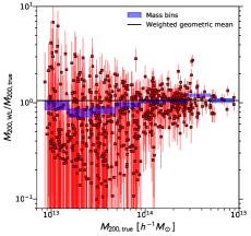
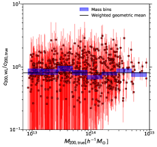
Furthermore, we have tested our shear fitting procedures and pipeline using the standard halo model including the effects of surrounding large-scale structure as a 2-halo term (Equation (26)). We describe the projected halo model with $M_{200}$ and $c_{200}$ as fitting parameters and use the same priors as for the NFW model. As demonstrated in Figure 4, the 2-halo term $\Delta\Sigma_{\mathrm{2h}}(R)$ is negligibly small in the comoving radial range $R\in[0.3,3]\,h^{-1}\mathrm{Mpc}$. When the 2-halo term is neglected, the halo model reduces to the BMO model that describes a smoothly truncated NFW profile (Section 4.4).

The results are summarized in Figure 18 and Table 6. Overall, the two-parameter halo modeling of each individual cluster does not significantly improve the accuracy of weak-lensing measurements of cluster mass and concentration, although it yields slightly ($<1\sigma$) improved levels of accuracy in the determination of $M_{500}$ and $M_{200}$.

Appendix B Marginalized Posterior Constraints on Regression Parameters

Figure 19.— Marginalized one-dimensional (histograms) and two-dimensional ($68\%$ and $95\%$ confidence level contour plots) posterior distributions of the regression parameters for the $c_{200}$–$M_{200}$ relation of the BAHAMAS sample at $z=0.25$, recovered from synthetic weak-lensing measurements (see Figure 17). For each parameter, the blue solid line shows the biweight central location ($C_{\mathrm{BI}}$) of the marginalized one-dimensional distribution. The left panel is for the full BAHAMAS sample of 639 halos (Figure 15), and the right panel is for a subsample of 459 halos that lie within $1\sigma$ scatter from the mean $c_{200}$–$M_{200}$ relation.

Figure 20.— Constraints on the regression parameters for the $c_{200}$–$M_{200}$ relation of the XXL sample, showing marginalized one-dimensional (histograms) and two-dimensional ($68\%$ and $95\%$ confidence level contour plots) posterior distributions. For each parameter, the blue solid line shows the biweight central location ($C_{\mathrm{BI}}$) of the marginalized one-dimensional distribution.

Figure 21.— Constraints on the regression parameters for the $T_{\mathrm{300\,kpc}}$–$M_{500}$ relation of the XXL sample, showing marginalized one-dimensional (histograms) and two-dimensional ($68\%$ and $95\%$ confidence level contour plots) posterior distributions. For each parameter, the blue solid line shows the biweight central location ($C_{\mathrm{BI}}$) of the marginalized one-dimensional distribution.

In Figure 19, we show marginalized one- and two-dimensional posterior probability distributions of the regression parameters $(\alpha_{Y|Z},\beta_{Y|Z},\sigma_{Y|Z},\sigma_{X|Z})$ for the $c_{200}$–$M_{200}$ relation of the BAHAMAS sample (Figure 14) recovered from the synthetic weak-lensing measurements shown in Figure 17 (for details, see Appendix A.2).

In Figures 20 and 21, we show marginalized posterior probability distributions of the regression parameters for the $c_{200}$–$M_{200}$ relation (Section 5.2) and the $T_{\mathrm{300\,kpc}}$–$M_{500}$ relation (Section 5.3), respectively, derived for the XXL cluster population.

References

- Adami et al. (2018) Adami, C., Giles, P., Koulouridis, E., et al. 2018, A&A, 620, A5, (XXL Paper XX)
- Aihara et al. (2018a) Aihara, H., Armstrong, R., Bickerton, S., et al. 2018a, PASJ, 70, S8
- Aihara et al. (2018b) Aihara, H., Arimoto, N., Armstrong, R., et al. 2018b, PASJ, 70, S4
- Allen et al. (2004) Allen, S. W., Schmidt, R. W., Ebeling, H., Fabian, A. C., & van Speybroeck, L. 2004, MNRAS, 353, 457
- Andreon & Bergé (2012) Andreon, S., & Bergé, J. 2012, A&A, 547, A117
- Applegate et al. (2014) Applegate, D. E., von der Linden, A., Kelly, P. L., et al. 2014, MNRAS, 439, 48
- Baltz et al. (2009) Baltz, E. A., Marshall, P., & Oguri, M. 2009, J. Cosmology Astropart. Phys, 1, 15
- Bartelmann & Schneider (2001) Bartelmann, M., & Schneider, P. 2001, Phys. Rep., 340, 291
- Becker & Kravtsov (2011) Becker, M. R., & Kravtsov, A. V. 2011, ApJ, 740, 25
- Beers et al. (1990) Beers, T. C., Flynn, K., & Gebhardt, K. 1990, AJ, 100, 32
- Benitez et al. (2014) Benitez, N., Dupke, R., Moles, M., et al. 2014, ArXiv e-prints, arXiv:1403.5237 [astro-ph.CO]
- Bertone & Tait (2018) Bertone, G., & Tait, T. M. P. 2018, Nature, 562, 51
- Bertschinger (1985) Bertschinger, E. 1985, ApJS, 58, 39
- Bhattacharya et al. (2013) Bhattacharya, S., Habib, S., Heitmann, K., & Vikhlinin, A. 2013, ApJ, 766, 32
- Biviano et al. (2013) Biviano, A., Rosati, P., Balestra, I., et al. 2013, A&A, 558, A1
- Biviano et al. (2017) Biviano, A., Moretti, A., Paccagnella, A., et al. 2017, A&A, 607, A81
- Bleem et al. (2015) Bleem, L. E., Stalder, B., de Haan, T., et al. 2015, ApJS, 216, 27
- Bosch et al. (2018) Bosch, J., Armstrong, R., Bickerton, S., et al. 2018, PASJ, 70, S5
- Broadhurst et al. (2005) Broadhurst, T., Takada, M., Umetsu, K., et al. 2005, ApJ, 619, L143
- Bulbul et al. (2019) Bulbul, E., Chiu, I. N., Mohr, J. J., et al. 2019, ApJ, 871, 50
- Buote et al. (2007) Buote, D. A., Gastaldello, F., Humphrey, P. J., et al. 2007, ApJ, 664, 123
- Child et al. (2018) Child, H. L., Habib, S., Heitmann, K., et al. 2018, ApJ, 859, 55
- Cibirka et al. (2017) Cibirka, N., Cypriano, E. S., Brimioulle, F., et al. 2017, MNRAS, 468, 1092
- Clowe et al. (2006) Clowe, D., Bradač, M., Gonzalez, A. H., et al. 2006, ApJ, 648, L109
- Clowe et al. (2004) Clowe, D., Gonzalez, A., & Markevitch, M. 2004, ApJ, 604, 596
- Coupon et al. (2018) Coupon, J., Czakon, N., Bosch, J., et al. 2018, PASJ, 70, S7
- Covone et al. (2014) Covone, G., Sereno, M., Kilbinger, M., & Cardone, V. F. 2014, ApJ, 784, L25
- Czakon et al. (2015) Czakon, N. G., Sayers, J., Mantz, A., et al. 2015, ApJ, 806, 18
- De Boni et al. (2013) De Boni, C., Ettori, S., Dolag, K., & Moscardini, L. 2013, MNRAS, 428, 2921
- Diemer & Joyce (2019) Diemer, B., & Joyce, M. 2019, ApJ, 871, 168
- Diemer & Kravtsov (2014) Diemer, B., & Kravtsov, A. V. 2014, ApJ, 789, 1
- Diemer & Kravtsov (2015) —. 2015, ApJ, 799, 108
- Donahue et al. (2014) Donahue, M., Voit, G. M., Mahdavi, A., et al. 2014, ApJ, 794, 136
- Dorman et al. (2003) Dorman, B., Arnaud, K. A., & Gordon, C. A. 2003, in Bulletin of the American Astronomical Society, Vol. 35, AAS/High Energy Astrophysics Division #7, 641
- Du et al. (2015) Du, W., Fan, Z., Shan, H., et al. 2015, ApJ, 814, 120
- Duffy et al. (2008) Duffy, A. R., Schaye, J., Kay, S. T., & Dalla Vecchia, C. 2008, MNRAS, 390, L64
- Dutton & Macciò (2014) Dutton, A. A., & Macciò, A. V. 2014, MNRAS, 441, 3359
- Eckert et al. (2011) Eckert, D., Molendi, S., & Paltani, S. 2011, A&A, 526, A79
- Eckert et al. (2014) Eckert, D., Molendi, S., Owers, M., et al. 2014, A&A, 570, A119
- Eckert et al. (2016) Eckert, D., Ettori, S., Coupon, J., et al. 2016, A&A, 592, A12, (XXL Paper XIII)
- Erben et al. (2013) Erben, T., Hildebrandt, H., Miller, L., et al. 2013, MNRAS, 433, 2545
- Ettori (2015) Ettori, S. 2015, MNRAS, 446, 2629
- Ettori et al. (2010) Ettori, S., Gastaldello, F., Leccardi, A., et al. 2010, A&A, 524, A68
- Farahi et al. (2018) Farahi, A., Guglielmo, V., Evrard, A. E., et al. 2018, A&A, 620, A8, (XXL Paper XXIII)
- Fasano et al. (2006) Fasano, G., Marmo, C., Varela, J., et al. 2006, A&A, 445, 805
- Fujita et al. (2018a) Fujita, Y., Umetsu, K., Ettori, S., et al. 2018a, ApJ, 863, 37
- Fujita et al. (2018b) Fujita, Y., Umetsu, K., Rasia, E., et al. 2018b, ApJ, 857, 118
- Furusawa et al. (2018) Furusawa, H., Koike, M., Takata, T., et al. 2018, PASJ, 70, S3
- Gruen et al. (2015) Gruen, D., Seitz, S., Becker, M. R., Friedrich, O., & Mana, A. 2015, MNRAS, 449, 4264
- Gruen et al. (2014) Gruen, D., Seitz, S., Brimioulle, F., et al. 2014, MNRAS, 442, 1507
- Gullieuszik et al. (2015) Gullieuszik, M., Poggianti, B., Fasano, G., et al. 2015, A&A, 581, A41
- Haiman et al. (2001) Haiman, Z., Mohr, J. J., & Holder, G. P. 2001, ApJ, 553, 545
- Hamana et al. (2020) Hamana, T., Shirasaki, M., Miyazaki, S., et al. 2020, PASJ, 72, 16
- Hattori et al. (1999) Hattori, M., Kneib, J., & Makino, N. 1999, Progress of Theoretical Physics Supplement, 133, 1
- Heymans et al. (2012) Heymans, C., Van Waerbeke, L., Miller, L., et al. 2012, MNRAS, 427, 146
- Hikage et al. (2019) Hikage, C., Oguri, M., Hamana, T., et al. 2019, PASJ, 71, 43
- Hinshaw et al. (2013) Hinshaw, G., Larson, D., Komatsu, E., et al. 2013, ApJS, 208, 19
- Hirata & Seljak (2003) Hirata, C., & Seljak, U. 2003, MNRAS, 343, 459
- Hjorth & Williams (2010) Hjorth, J., & Williams, L. L. R. 2010, ApJ, 722, 851
- Hoekstra (2003) Hoekstra, H. 2003, MNRAS, 339, 1155
- Hoekstra et al. (2015) Hoekstra, H., Herbonnet, R., Muzzin, A., et al. 2015, MNRAS, 449, 685
- Ilbert et al. (2009) Ilbert, O., Capak, P., Salvato, M., et al. 2009, ApJ, 690, 1236
- Israel et al. (2015) Israel, H., Schellenberger, G., Nevalainen, J., Massey, R., & Reiprich, T. H. 2015, MNRAS, 448, 814
- Jing & Suto (2000) Jing, Y. P., & Suto, Y. 2000, ApJ, 529, L69
- Jing & Suto (2002) —. 2002, ApJ, 574, 538
- Johnston et al. (2007) Johnston, D. E., Sheldon, E. S., Wechsler, R. H., et al. 2007, ArXiv e-prints, arXiv:0709.1159
- Kaiser (1986) Kaiser, N. 1986, MNRAS, 222, 323
- Kaiser (1995) —. 1995, ApJ, 439, L1
- Kawanomoto et al. (2018) Kawanomoto, S., Uraguchi, F., Komiyama, Y., et al. 2018, PASJ, 70, 66
- Kelly (2007) Kelly, B. C. 2007, ApJ, 665, 1489
- Kettula et al. (2015) Kettula, K., Giodini, S., van Uitert, E., et al. 2015, MNRAS, 451, 1460
- Klein et al. (2019) Klein, M., Israel, H., Nagarajan, A., et al. 2019, MNRAS, 488, 1704
- Klypin et al. (2016) Klypin, A., Yepes, G., Gottlöber, S., Prada, F., & Heß, S. 2016, MNRAS, 457, 4340
- Komatsu et al. (2009) Komatsu, E., Dunkley, J., Nolta, M. R., et al. 2009, ApJS, 180, 330
- Komiyama et al. (2018) Komiyama, Y., Obuchi, Y., Nakaya, H., et al. 2018, PASJ, 70, S2
- Laigle et al. (2016) Laigle, C., McCracken, H. J., Ilbert, O., et al. 2016, ApJS, 224, 24
- Lavoie et al. (2016) Lavoie, S., Willis, J. P., Démoclès, J., et al. 2016, MNRAS, 462, 4141, (XXL Paper XV)
- Leauthaud et al. (2010) Leauthaud, A., Finoguenov, A., Kneib, J.-P., et al. 2010, ApJ, 709, 97
- Lieu et al. (2017) Lieu, M., Farr, W. M., Betancourt, M., et al. 2017, MNRAS, 468, 4872
- Lieu et al. (2016) Lieu, M., Smith, G. P., Giles, P. A., et al. 2016, A&A, 592, A4, (XXL Paper IV)
- Mandelbaum et al. (2005a) Mandelbaum, R., Tasitsiomi, A., Seljak, U., Kravtsov, A. V., & Wechsler, R. H. 2005a, MNRAS, 362, 1451
- Mandelbaum et al. (2005b) Mandelbaum, R., Hirata, C. M., Seljak, U., et al. 2005b, MNRAS, 361, 1287
- Mandelbaum et al. (2008) Mandelbaum, R., Seljak, U., Hirata, C. M., et al. 2008, MNRAS, 386, 781
- Mandelbaum et al. (2018a) Mandelbaum, R., Miyatake, H., Hamana, T., et al. 2018a, PASJ, 70, S25
- Mandelbaum et al. (2018b) Mandelbaum, R., Lanusse, F., Leauthaud, A., et al. 2018b, MNRAS, 481, 3170
- Mantz et al. (2010) Mantz, A., Allen, S. W., Rapetti, D., & Ebeling, H. 2010, MNRAS, 406, 1759
- Mantz et al. (2016) Mantz, A. B., Allen, S. W., Morris, R. G., & Schmidt, R. W. 2016, MNRAS, 456, 4020
- Marulli et al. (2018) Marulli, F., Veropalumbo, A., Sereno, M., et al. 2018, A&A, 620, A1, (XXL Paper XVI)
- Masters et al. (2015) Masters, D., Capak, P., Stern, D., et al. 2015, ApJ, 813, 53
- Maughan (2014) Maughan, B. J. 2014, MNRAS, 437, 1171
- McCarthy et al. (2018) McCarthy, I. G., Bird, S., Schaye, J., et al. 2018, MNRAS, 476, 2999
- McCarthy et al. (2017) McCarthy, I. G., Schaye, J., Bird, S., & Le Brun, A. M. C. 2017, MNRAS, 465, 2936
- Medezinski et al. (2010) Medezinski, E., Broadhurst, T., Umetsu, K., et al. 2010, MNRAS, 405, 257
- Medezinski et al. (2018a) Medezinski, E., Battaglia, N., Umetsu, K., et al. 2018a, PASJ, 70, S28
- Medezinski et al. (2018b) Medezinski, E., Oguri, M., Nishizawa, A. J., et al. 2018b, PASJ, 70, 30
- Melchior et al. (2015) Melchior, P., Suchyta, E., Huff, E., et al. 2015, MNRAS, 449, 2219
- Melchior et al. (2017) Melchior, P., Gruen, D., McClintock, T., et al. 2017, MNRAS, 469, 4899
- Meneghetti et al. (2014) Meneghetti, M., Rasia, E., Vega, J., et al. 2014, ApJ, 797, 34
- Merten et al. (2015) Merten, J., Meneghetti, M., Postman, M., et al. 2015, ApJ, 806, 4
- Miyaoka et al. (2018) Miyaoka, K., Okabe, N., Kitaguchi, T., et al. 2018, PASJ, 70, S22
- Miyatake et al. (2019) Miyatake, H., Battaglia, N., Hilton, M., et al. 2019, ApJ, 875, 63
- Miyazaki et al. (2018a) Miyazaki, S., Oguri, M., Hamana, T., et al. 2018a, PASJ, 70, S27
- Miyazaki et al. (2018b) Miyazaki, S., Komiyama, Y., Kawanomoto, S., et al. 2018b, PASJ, 70, S1
- Morandi et al. (2012) Morandi, A., Limousin, M., Sayers, J., et al. 2012, MNRAS, 425, 2069
- Nakajima et al. (2012) Nakajima, R., Mandelbaum, R., Seljak, U., et al. 2012, MNRAS, 420, 3240
- Navarro et al. (1996) Navarro, J. F., Frenk, C. S., & White, S. D. M. 1996, ApJ, 462, 563
- Navarro et al. (1997) —. 1997, ApJ, 490, 493
- Neto et al. (2007) Neto, A. F., Gao, L., Bett, P., et al. 2007, MNRAS, 381, 1450
- Newman et al. (2013) Newman, A. B., Treu, T., Ellis, R. S., et al. 2013, ApJ, 765, 24
- Niikura et al. (2015) Niikura, H., Takada, M., Okabe, N., Martino, R., & Takahashi, R. 2015, PASJ, 67, 103
- Oguri (2014) Oguri, M. 2014, MNRAS, 444, 147
- Oguri et al. (2012) Oguri, M., Bayliss, M. B., Dahle, H., et al. 2012, MNRAS, 420, 3213
- Oguri & Hamana (2011) Oguri, M., & Hamana, T. 2011, MNRAS, 414, 1851
- Oguri et al. (2005) Oguri, M., Takada, M., Umetsu, K., & Broadhurst, T. 2005, ApJ, 632, 841
- Oguri et al. (2018) Oguri, M., Lin, Y.-T., Lin, S.-C., et al. 2018, PASJ, 70, S20
- Okabe & Smith (2016) Okabe, N., & Smith, G. P. 2016, MNRAS, 461, 3794
- Okabe et al. (2013) Okabe, N., Smith, G. P., Umetsu, K., Takada, M., & Futamase, T. 2013, ApJ, 769, L35
- Okabe & Umetsu (2008) Okabe, N., & Umetsu, K. 2008, PASJ, 60, 345
- Okabe et al. (2019) Okabe, N., Oguri, M., Akamatsu, H., et al. 2019, PASJ, 71, 79
- Okabe et al. (2018) Okabe, T., Nishimichi, T., Oguri, M., et al. 2018, MNRAS, 478, 1141
- Pacaud et al. (2016) Pacaud, F., Clerc, N., Giles, P. A., et al. 2016, A&A, 592, A2, (XXL Paper II)
- Pacaud et al. (2018) Pacaud, F., Pierre, M., Melin, J.-B., et al. 2018, A&A, 620, A10, (XXL Paper XXV)
- Pierre et al. (2016) Pierre, M., Pacaud, F., Adami, C., et al. 2016, A&A, 592, A1, (XXL Paper I)
- Planck Collaboration et al. (2014) Planck Collaboration, Ade, P. A. R., Aghanim, N., et al. 2014, A&A, 571, A20
- Planck Collaboration et al. (2016) —. 2016, A&A, 594, A24
- Postman et al. (2012) Postman, M., Coe, D., Benítez, N., et al. 2012, ApJS, 199, 25
- Pratt et al. (2019) Pratt, G. W., Arnaud, M., Biviano, A., et al. 2019, Space Sci. Rev., 215, 25
- Ragagnin et al. (2019) Ragagnin, A., Dolag, K., Moscardini, L., Biviano, A., & D’Onofrio, M. 2019, MNRAS, 486, 4001
- Randall et al. (2008) Randall, S. W., Markevitch, M., Clowe, D., Gonzalez, A. H., & Bradač, M. 2008, ApJ, 679, 1173
- Rasia et al. (2013) Rasia, E., Borgani, S., Ettori, S., Mazzotta, P., & Meneghetti, M. 2013, ApJ, 776, 39
- Ricker & Sarazin (2001) Ricker, P. M., & Sarazin, C. L. 2001, ApJ, 561, 621
- Rossetti et al. (2017) Rossetti, M., Gastaldello, F., Eckert, D., et al. 2017, MNRAS, 468, 1917
- Rykoff et al. (2016) Rykoff, E. S., Rozo, E., Hollowood, D., et al. 2016, ApJS, 224, 1
- Schneider & Seitz (1995) Schneider, P., & Seitz, C. 1995, A&A, 294, 411
- Schrabback et al. (2018) Schrabback, T., Applegate, D., Dietrich, J. P., et al. 2018, MNRAS, 474, 2635
- Sereno (2016a) Sereno, M. 2016a, MNRAS, 455, 2149
- Sereno (2016b) —. 2016b, LIRA: LInear Regression in Astronomy, Astrophysics Source Code Library, ascl:1602.006
- Sereno & Covone (2013) Sereno, M., & Covone, G. 2013, MNRAS, 434, 878
- Sereno et al. (2017) Sereno, M., Covone, G., Izzo, L., et al. 2017, MNRAS, 472, 1946
- Sereno & Ettori (2015a) Sereno, M., & Ettori, S. 2015a, MNRAS, 450, 3675
- Sereno & Ettori (2015b) —. 2015b, MNRAS, 450, 3633
- Sereno & Ettori (2017) —. 2017, MNRAS, 468, 3322
- Sereno et al. (2015a) Sereno, M., Ettori, S., & Moscardini, L. 2015a, MNRAS, 450, 3649
- Sereno et al. (2013) Sereno, M., Ettori, S., Umetsu, K., & Baldi, A. 2013, MNRAS, 428, 2241
- Sereno & Umetsu (2011) Sereno, M., & Umetsu, K. 2011, MNRAS, 416, 3187
- Sereno et al. (2018) Sereno, M., Umetsu, K., Ettori, S., et al. 2018, ApJ, 860, L4
- Sereno et al. (2015b) Sereno, M., Veropalumbo, A., Marulli, F., et al. 2015b, MNRAS, 449, 4147
- Sereno et al. (2020) Sereno, M., Umetsu, K., Ettori, S., et al. 2020, MNRAS, 492, 4528
- Smith et al. (2003) Smith, R. E., Peacock, J. A., Jenkins, A., et al. 2003, MNRAS, 341, 1311
- Stanford et al. (1998) Stanford, S. A., Eisenhardt, P. R., & Dickinson, M. 1998, ApJ, 492, 461
- Tanaka et al. (2018) Tanaka, M., Coupon, J., Hsieh, B.-C., et al. 2018, PASJ, 70, S9
- Taylor & Navarro (2001) Taylor, J. E., & Navarro, J. F. 2001, ApJ, 563, 483
- Tinker et al. (2010) Tinker, J. L., Robertson, B. E., Kravtsov, A. V., et al. 2010, ApJ, 724, 878
- Umetsu (2010) Umetsu, K. 2010, ArXiv e-prints, arXiv:1002.3952 [astro-ph.CO]
- Umetsu & Broadhurst (2008) Umetsu, K., & Broadhurst, T. 2008, ApJ, 684, 177
- Umetsu et al. (2011a) Umetsu, K., Broadhurst, T., Zitrin, A., et al. 2011a, ApJ, 738, 41
- Umetsu et al. (2011b) Umetsu, K., Broadhurst, T., Zitrin, A., Medezinski, E., & Hsu, L. 2011b, ApJ, 729, 127
- Umetsu & Diemer (2017) Umetsu, K., & Diemer, B. 2017, ApJ, 836, 231
- Umetsu et al. (2016) Umetsu, K., Zitrin, A., Gruen, D., et al. 2016, ApJ, 821, 116
- Umetsu et al. (2012) Umetsu, K., Medezinski, E., Nonino, M., et al. 2012, ApJ, 755, 56
- Umetsu et al. (2014) —. 2014, ApJ, 795, 163
- Umetsu et al. (2015) Umetsu, K., Sereno, M., Medezinski, E., et al. 2015, ApJ, 806, 207
- Umetsu et al. (2018) Umetsu, K., Sereno, M., Tam, S.-I., et al. 2018, ApJ, 860, 104
- Vikhlinin et al. (2009a) Vikhlinin, A., Burenin, R. A., Ebeling, H., et al. 2009a, ApJ, 692, 1033
- Vikhlinin et al. (2009b) Vikhlinin, A., Kravtsov, A. V., Burenin, R. A., et al. 2009b, ApJ, 692, 1060
- von der Linden et al. (2014) von der Linden, A., Allen, M. T., Applegate, D. E., et al. 2014, MNRAS, 439, 2
- Watson et al. (2014) Watson, W. A., Iliev, I. T., Diego, J. M., et al. 2014, MNRAS, 437, 3776
- Williams & Hjorth (2010) Williams, L. L. R., & Hjorth, J. 2010, ApJ, 722, 856
- Wright & Brainerd (2000) Wright, C. O., & Brainerd, T. G. 2000, ApJ, 534, 34
- Zhang et al. (2016) Zhang, C., Yu, Q., & Lu, Y. 2016, ApJ, 820, 85