FENCE: Feasible Evasion Attacks on Neural Networks in Constrained Environments

Abstract.

As advances in Deep Neural Networks (DNNs) demonstrate unprecedented levels of performance in many critical applications, their vulnerability to attacks is still an open question. We consider evasion attacks at testing time against Deep Learning in constrained environments, in which dependencies between features need to be satisfied. These situations may arise naturally in tabular data or may be the result of feature engineering in specific application domains, such as threat detection in cyber security. We propose a general iterative gradient-based framework called FENCE for crafting evasion attacks that take into consideration the specifics of constrained domains and application requirements. We apply it against Feed-Forward Neural Networks trained for two cyber security applications: network traffic botnet classification and malicious domain classification, to generate feasible adversarial examples. We extensively evaluate the success rate and performance of our attacks, compare their improvement over several baselines, and analyze factors that impact the attack success rate, including the optimization objective and the data imbalance. We show that with minimal effort (e.g., generating 12 additional network connections), an attacker can change the model’s prediction from the Malicious class to Benign and evade the classifier. We show that models trained on datasets with higher imbalance are more vulnerable to our FENCE attacks. Finally, we demonstrate the potential of performing adversarial training in constrained domains to increase the model resilience against these evasion attacks.

1. Introduction

Deep learning has reached high performance in machine learning (ML) tasks in a variety of application domains, including image classification, speech recognition, and natural language processing (NLP). Many applications already benefit from the deployment of ML for automating decisions and we expect a proliferation of ML in even more critical settings in the near future. Still, research in adversarial machine learning showed that deep neural networks (DNNs) are not robust in face of adversarial attacks. The first adversarial attack against DNNs was an evasion attack, in which an adversary creates adversarial examples that minimally perturb testing samples and change the classifier’s prediction (Szegedy et al., 2014). Since the discovery of adversarial examples in computer vision, a lot of work on evasion attacks against ML classifiers at deployment time has been performed. Most of these attacks have been demonstrated in continuous domains (i.e., image classification), in which features or image pixels can be modified arbitrarily to create the perturbations (Szegedy et al., 2014; Biggio et al., 2013; Goodfellow et al., 2014; Kurakin et al., 2016; Papernot et al., 2017b; Carlini and Wagner, 2017; Madry et al., 2017; Athalye et al., 2018).

ML has a lot of potential in other application domains, including cyber security, finance, and healthcare, in which the raw data is not directly suitable for learning and engineered features are defined by domain experts to train DNN models. Additionally, in certain application domains such as network traffic classification used in cyber security, the raw data itself might exhibit domain-specific constraints in the original input space. Therefore, techniques used for mounting evasion attacks in continuous domains will not respect the feature-space dependencies in these applications and new adversarial attacks need to be designed for such constrained domains.

In this paper we introduce a novel, general framework for mounting evasion attacks against deep learning models in constrained application domains. Our framework is named FENCE (Feasible Evasion Attacks on Neural Networks in Constrained Environments). FENCE generates feasible adversarial examples in constrained domains that rely either on feature engineering or naturally have domain-specific dependencies in the input space. FENCE supports a range of linear and non-linear dependencies in feature space and can be applied to any higher-level classification task whose data respects these constraints. At the core of FENCE is an iterative optimization method that determines the feature of the maximum gradient of the attacker’s objective at each iteration, identifies the family of features dependent on that feature, and modifies consistently all those features, while preserving an upper bound on the maximum distance from the original sample. At any time during the iterative procedure, the input data point is modified within the feasibility region, resulting in feasible adversarial examples. Existing evasion attacks in constrained environments, such as PDF malware detection (Srndic and Laskov, 2014; Tong et al., 2019), malware classification (Grosse et al., 2016; Suciu et al., 2018a), and network traffic classification  (Alhajjar et al., 2020; Granados et al., 2020; Abusnaina et al., 2019; Han et al., 2020; Sadeghzadeh et al., 2021) do not support the entire range of complex mathematical and domain-specific dependencies as our FENCE framework. Moreover, some of these attacks result in worse performance (Alhajjar et al., 2020) or operate only in a specific domain (Sadeghzadeh et al., 2021) or feature space (Alhajjar et al., 2020; Granados et al., 2020).

We demonstrate that FENCE can successfully evade the DNNs trained for two cyber security applications: a malicious network traffic classifier using the CTU-13 botnet dataset (Garcia et al., 2014), and a malicious domain classifier using the MADE system (Oprea et al., 2018). In both settings, FENCE generates feasible adversarial examples with small modification of the original testing sample. For instance, by adding 12 network connections and preserving the original malicious behavior, an attacker can change the classification prediction of a testing sample from $\mathsf{Malicious}$ to $\mathsf{Benign}$ in the network traffic classifier. We perform detailed evaluation to demonstrate that our attacks perform better than several baselines and existing attacks. We show that the state-of-the-art Carlini-Wagner attack (Carlini and Wagner, 2017) designed for continuous domains does not respect the feature-space dependencies of our security applications. We compare two optimization objectives in our FENCE framework, the Projected Gradient Descent (PGD) (Madry et al., 2017) and the Penalty method (Carlini and Wagner, 2017), and show the advantages of the PGD optimization. We also study the impact of data imbalance on the classifier robustness and show that models trained on datasets with higher imbalance, as is common in security applications, are more vulnerable.

We also consider attack models with minimum knowledge about the ML system, in which the attacker does not have information about the exact model architecture and hyperparameters. We test several approaches for performing the attacks through transferability from a surrogate model to the original one, using the FENCE framework. We observe that the evasion attacks generated for different DNN architectures transfer to the target DNN model with slightly lower success than attacking directly the target model with FENCE. Finally, we test the resilience of adversarial training using our attacks as a defensive mechanism for DNNs trained in constrained environments.

To summarize, our contributions are:

1. We introduce a general evasion attack framework FENCE for constrained application domains that supports a range of mathematical dependencies in feature space and two optimization approaches.

2. We apply FENCE to two cyber security applications using different datasets and feature representations: a malicious network connection classifier, and a malicious domain detector, to generate feasible adversarial examples in these domains.

3. We extensively evaluate FENCE for these applications, compare our attacks with several baselines, and quantify the adversarial success at different perturbations. We also study the impact of data imbalance on the classifiers’ robustness.

4. We evaluate the transferability of the proposed evasion attacks between different ML models and architectures, and show that adversarially-trained models provide higher robustness.

2. Background

2.1. Deep Neural Networks for Classification

A feed-forward neural network (FFNN) for binary classification is a function $y=F(x)$ from input $x\in R^{d}$ (of dimension $d$) to output $y\in\{0,1\}$. The parameter vector of the function is learned during the training phase using back propagation over the network layers. Each layer includes a matrix multiplication and non-linear activation (e.g., ReLU). The last layer’s activation is sigmoid $\sigma$ for binary classification: $y=F(x)=\sigma(Z(x))$, where $Z(x)$ are the logits, i.e., the output of the penultimate layer. We denote by $C(x)$ the predicted class for $x$. For multi-class classification, the last layer uses a softmax activation function. There are other DNN architectures for classification, such as convolutional neural networks, but in this paper we only consider FFNN architectures.

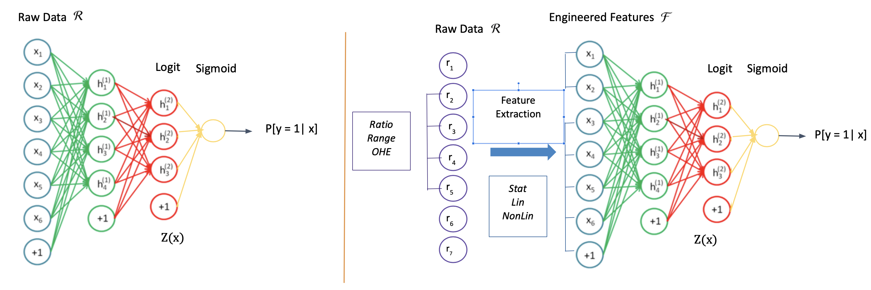
Figure 1. Neural network training for images (left) and for constrained domains with feature space dependencies (right). In the vision domain the raw data space $\mathcal{R}$ is the same as the feature representation $\mathcal{F}$, while in constrained domains they might be different. Additional dependencies in feature space might arise from natural dependencies in the raw data and the feature engineering process.

2.2. Threat Model

Adversarial attacks against ML algorithms can be developed in the training or testing phase. In this work, we consider testing-time attacks, called evasion attacks. There exist several evasion attacks against DNNs in continuous domains: the projected gradient descent (PGD) attack (Madry et al., 2017) and the penalty-based attack of Carlini and Wagner (Carlini and Wagner, 2017).

Projected gradient attacks. This is a class of attacks based on gradient descent for objective minimization, that project the adversarial points to the feasible domain at each iteration. For instance, Biggio et al. (Biggio et al., 2013) use an objective that maximizes the confidence of adversarial examples, within a ball of fixed radius in $L_{1}$ norm. Madry et al. (Madry et al., 2017) use the loss function directly as the optimization objective and use the $L_{2}$ and $L_{\infty}$ distances for projection.

C&W attack. Carlini and Wagner (Carlini and Wagner, 2017) solve the following optimization problem to create adversarial examples against CNNs used for multi-class prediction:

$\delta=\operatorname{arg\,min}||\delta||_{2}+c\cdot h(x+\delta)$

$h(x+\delta)=\max(0,\max(Z_{k}(x+\delta):k\neq t)-Z_{t}(x+\delta))$,

where $Z()$ are the logits of the FFNN.

This is called the penalty method, and the optimization objective has two terms: the norm of the perturbation $\delta$, and a function $h(x+\delta)$ that is minimized when the adversarial example $x+\delta$ is classified as the target class $t$. The attack works for $L_{0}$, $L_{2}$, and $L_{\infty}$ norms.

Under the assumption that the DNN model is trained correctly, the attacker’s goal is to create adversarial examples at testing time. In security settings, typically the attacker starts with $\mathsf{Malicious}$ points that he aims to minimally modify into adversarial examples classified as $\mathsf{Benign}$.

Initially, we consider a white-box attack model, in which the attacker has full knowledge of the ML system. White-box attacks have been considered extensively in previous work, e.g., (Goodfellow et al., 2014; Biggio et al., 2013; Carlini and Wagner, 2017; Madry et al., 2017) to evaluate the robustness of existing ML classification algorithms. We also consider a more realistic attack model, in which the attacker has information about the feature representation of the underlying classifier, but no exact details on the ML algorithm and training data.

We address application domains with various constraints in feature space. These could manifest directly in the raw data features or could be an artifact of the feature engineering process. The attacker has the ability to insert records in the raw data, for instance by inserting network connections in the threat detection applications. We ensure that the data points modified or added by the attacker are feasible in the constrained domain.

3. Methodology

In this section, we start by describing the classification setting in constrained domains with dependencies in feature space and the challenges of evasion attacks in this setting. Then we devote the majority of the section to present our new attack framework FENCE which takes into consideration the relationships between features that occur naturally in the problem space or are the result of feature engineering.

3.1. Machine Learning Classification in Constrained Domains

Let the raw data input space be denoted as $\mathcal{R}$. This is the original space in which raw data is collected for an application. In healthcare, $\mathcal{R}$ could be the space of all data collected for a particular patient. In network security, $\mathcal{R}$ could be the raw network traffic (for example, pcap files or Zeek network logs) collected in a monitored network in order to detect cyber attacks.

Consider a fixed raw data set $R=\{r_{1},\dots,r_{M}\}\in\mathcal{R}$. The raw data is typically processed into a feature representation, denoted by $\mathcal{F}$, over which the machine learning model is trained. In standard computer vision tasks such as image classification, the raw data (image pixels) is used directly as input for neural networks. Thus, the training examples $x_{i}$ are the same as the raw data: $x_{i}=r_{i},i\in[1,M]$. In this case the feature space $\mathcal{F}$ is the same as the input space $\mathcal{R}$.

In contrast, in other domains, such as threat detection or health care, the feature representation is not always exactly the raw data. See Figure 1 for a visual representation of this process. In most application domains, there might exist dependencies and constraints in the feature space introduced either by the application itself or by the feature engineering process:

• Dependencies among different features could manifest naturally in the considered application. For instance, the results of two blood tests are correlated and they result in correlated feature values for a patient data. In network security, the packet size and number of packets are correlated with the total number of bytes sent in a TCP connection. We denote by $\mathsf{Feasible\_Set}(R)$ the set of all feasible points in the raw data space. $\mathsf{Feasible\_Set}(R)$ is a subset of the raw data that encompasses the feasible values for the particular application. For instance, a network TCP packet size is upper bounded by 1500 bytes and the ratio between the number of bytes and the number of packets in a TCP connection needs to be lower than the maximum packet size. The feasible set $\mathsf{Feasible\_Set}(R)$ will only include network connections in which the upper bound on TCP packets is enforced and the ratio constraint between the number of bytes and number of packets is satisfied.

• Constraints in feature representations might also result from the feature engineering process performed in many settings. In this case, features in $\mathcal{F}$ are obtained by the application of an operator $\mathsf{Op}_{j}$ on the raw data $R\in\mathcal{R}$: $x_{ij}=\mathsf{Op}_{j}(R)$. Examples of operators are statistical functions such as $\mathsf{Max}$, $\mathsf{Min}$, $\mathsf{Avg}$, and $\mathsf{Total}$, as well as linear combinations of raw data values, and other mathematical functions such as product or ratio of two values. The set of all supported operators applied to the raw data is denoted by $\mathcal{O}$. This process creates $N$ training examples $x_{1},\dots,x_{N}$ in the feature space $\mathcal{F}$, each being $d$-dimensional, with $d$ the size of the feature space. The feature engineering process creates additional dependencies in feature space. For instance, if we consider the $\mathsf{Max}$, $\mathsf{Min}$, and $\mathsf{Avg}$ number of connections for a particular port in a given time window, the average value needs to be between the minimum and the maximum values.

A data point $z=(z_{1},\dots,z_{d})$ in feature space $\mathcal{F}$ is feasible if there exists some raw data $R\in\mathcal{R}$ such as for all $i$, there exists an operator $\mathsf{Op}_{j}\in\mathcal{O}$ with $z_{i}=\mathsf{Op}_{j}(R)$. The set of all feasible points in feature space for raw data $R$ and operators $\mathcal{O}$ is called $\mathsf{Feasible\_Set}(R,\mathcal{O})$. This space includes the set of feasible points $\mathsf{Feasible\_Set}(R)$ (obtained for $\mathcal{O}=\emptyset$). Examples of feasible and infeasible points in feature space are illustrated in Table 1. The constraints in this example are that the sum of feature values must sum up to one. This may arise in situations when the subset of features represents ratio values, for example, the ratio of connections that have a particular result code.

Feature	Feasible point	Infeasible point
$F_{1}$	0.2	0.5
$F_{2}$	0.13	0.13
$F_{3}$	0.33	0.33
$F_{4}$	0.34	0.4

Table 1. Example feature values for four ratio features, whose sum needs to be 1 in the feasibility region. We show an example of a feasible point and an infeasible one in feature space $\mathcal{F}$.

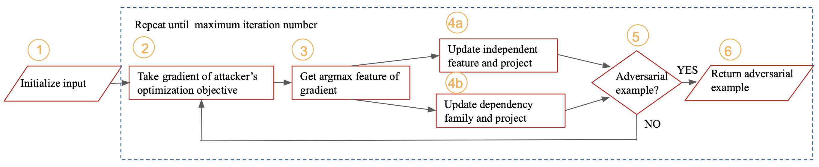
Figure 2. Flow of the FENCE Evasion Attack Framework.

3.2. Challenges

Existing evasion attacks are mostly designed for continuous domains, such as image classification, where adversarial examples have pixel values in a fixed range (e.g., [0,1]) and can be modified independently (Carlini and Wagner, 2017; Madry et al., 2017; Athalye et al., 2018). However, many applications in cyber security use tabular data, resulting in feature dependencies and physical-world constraints that need to be respected.

Several previous works address evasion attacks in domains with tabular data. The evasion attack for malware detection by Grosse et al. (Grosse et al., 2017), which directly leverages JSMA (Papernot et al., 2017b), modifies binary features corresponding to system calls. Kolosnjaji et al. (Kolosnjaji et al., 2018) use the attack of Biggio et al. (Biggio et al., 2013) to append selected bytes at the end of the malware file. Suciu et al. (Suciu et al., 2018a) also append bytes in selected regions of malicious files. Kulynych et al.  (Kulynych et al., 2018) introduce a graphical framework in which an adversary constructs all feasible transformations of an input, and then uses graph search to determine the path of the minimum cost to generate an adversarial example.

Neither of these approaches is applicable to our general setting because the attacks do not satisfy the required dependencies in the resulting adversarial vector. Crafting adversarial examples that are feasible, and respecting all the application constraints and dependencies poses a significant challenge. Once application constraints are specified, the resulting optimization problem for creating adversarial examples includes a number of non-linear constraints and cannot be solved directly using out-of-the-box optimization methods.

In order to measure the feasibility of adversarial examples, we run the existing Carlini and Wagner (C&W) attack (Carlini and Wagner, 2017) on a malicious domain classification. The details of the attack adaptation for this application are given in Section 4.2. We considered the balanced case, in which the number of $\mathsf{Malicious}$ and $\mathsf{Benign}$ examples is equal in training. While the attack reaches 98% success at a distance of 20, the resulting adversarial examples are outside the feasibility region. An example is included in Table 2, and the description of the features is given in Table 6. In this case, the average number of connections is not equal to the total number of connections divided by the number of IPs contacting the domain. Additionally, the average ratio of received bytes over sent bytes should be equal to the maximum and minimum values (as the number of IPs contacting the domain is 1).

Feature	Description	Input	Adversarial Example	Correct Value
Num_IP	Number of IPs	1	1	1
Num_Conn	Number of connections	15	233.56	233.56
Avg_Conns	Avg. connections by IP	15	59.94	233.56
Avg_Ratio_Bytes	Avg. ratio bytes	8.27	204.01	204.01
Max_Ratio_Bytes	Max. ratio bytes	8.27	240.02	204.01
Min_Ratio_Bytes	Min. ratio of bytes	8.27	119.12	204.01

Table 2. Infeasible C&W adversarial example for the malicious domain classifier. The inconsistent feature values are in red, while the correct values are in green. We consider all the IPs that connect to the domain and all the connections made to the domain. The ratio of bytes features are computed as ratio of received bytes over sent bytes per IP. When there is a single IP connecting to the domain, the number of connections should be equal to the average number of connections by IP, and the three ratio bytes features should all be equal.

3.3. The FENCE framework

To address these issues, we introduce the FENCE framework for evasion attacks that preserves a range of feature dependencies in constrained domains. FENCE guarantees by design that the produced adversarial examples are within the feasible region of the application input space.

The starting point for the attack framework are gradient-based optimization algorithms, including projected (Biggio et al., 2013; Madry et al., 2017) and penalty-based (Carlini and Wagner, 2017) optimization methods. Of course, we cannot apply these attacks directly since they will not preserve the feature dependencies. To overcome this, we use the values of the objective gradient at each iteration to select features of maximum gradient values. We create feature-update algorithms for each family of dependencies that use a combination of gradient-based method and mathematical constraints to always maintain a feasible point that satisfies the constraints. We also use various projection operators to project the updated adversarial examples to feasible regions of the feature space.

Algorithm 1 FENCE Framework for Evasion Attack with Constraints

0:  $\boldsymbol{x},y$: the input sample and its label; $t$: target label; $C$: prediction function; $G$: optimization objective; $d_{max}$: maximum allowed perturbation; $F_{S}$: subset of features that can be modified $F_{D}$: features in $F_{S}$ that have dependencies; $M$: maximum number of iterations; $\alpha$: learning rate.

0:  $\boldsymbol{x}^{*}$: adversarial example or $\bot$ if not successful.

1:  Initialize $m\leftarrow 0;x^{0}\leftarrow\boldsymbol{x}$

2:  // Iterate until successful or stopping condition

3:  while $C(x^{m})!=t$ and $m<M$  do

4:     $\nabla\leftarrow[\nabla G_{x_{i}}(x^{m})]_{i}$ // Gradient vector

5:     $\nabla_{S}\leftarrow\nabla_{F_{S}}$ // Gradients of features in $F_{S}$

6:     $i_{max}\leftarrow\mathsf{argmax}\nabla_{S}$ // Feature of max gradient

7:     // Check if feature has dependencies

8:     if $i_{max}\in F_{D}$ then

9:        // Update dependent features

10:        $x^{m+1}\leftarrow\mathsf{UPDATE\_FAMILY}(m,x^{m},\nabla,i_{max})$

11:     else

12:        Gradient update and projection

13:        $x_{i_{max}}^{m+1}\leftarrow x^{m}_{i_{max}}-\alpha\nabla_{i_{max}}$

14:        $x^{m+1}\leftarrow\Pi_{2}(x^{m+1})$

15:     end if

16:     $F_{S}\leftarrow F_{S}\setminus\{i_{max}\}$

17:     $m\leftarrow m+1$

18:     if $C(x^{m})=t$ then

19:        $x^{*}\leftarrow$ PROJECT_TO_RAW($x^{m}$)

20:        return  $x^{*}$

21:     end if

22:  end while

23:  return  $\bot$

Algorithm 2 $\mathsf{UPDATE\_FAMILY}$ ($m,x^{m},\nabla,i_{max}$)

1:  // Extract all dependent features on $i_{max}$

2:  $F_{i_{max}}\leftarrow\mathsf{Family\_Dep}(i_{max})$

3:  // Family representative feature

4:  $j\leftarrow\mathsf{Family\_Rep}(F_{i_{max}})$

5:  $\delta\leftarrow\nabla_{j}$ // Gradient of representative feature

6:  // Initialization function

7:  $s\leftarrow\mathsf{INIT\_FAMILY}(x^{m},\nabla,j)$

8:  // Binary search for perturbation

9:  while $\delta\neq 0$ do

10:     $x^{m}_{j}\leftarrow x^{m}_{j}-\alpha\delta$ // Gradient update

11:     $x^{m}\leftarrow\mathsf{UPDATE\_DEP}(s,x^{m},\nabla,F_{i_{max}})$

12:     if $d(x^{m},x^{0})>d_{max}$ then

13:        // Reduce perturbation

14:        $\delta\leftarrow\delta/2$

15:     else

16:        return  $x^{m}$

17:     end if

18:  end while

Algorithms 1, 2 and Figure 2 describe the general FENCE framework. We consider binary classifiers designed using FFNN architectures. However, the framework can be extended to multi-class scenarios by modifying the optimization objective. For measuring the amount of perturbation added by the original example, we use the $L_{2}$ norm.

The input to the FENCE framework consists of: an input sample $\boldsymbol{x}$ with label $y$ (typically $\mathsf{Malicious}$ in security applications); a target label $t$ (typically $\mathsf{Benign}$); the model prediction function $C$; the optimization objective $G$; maximum allowed perturbation $d_{max}$; the subset of features $F_{S}$ that can be modified; the features that have dependencies $F_{D}\subset F_{S}$; the maximum number of iterations $M$ and a learning rate $\alpha$ for gradient descent. The set of dependent features is split into families of features. A family is defined as a subset of $F_{D}$ such that features within the family need to be updated simultaneously, whereas features outside the family can be updated independently. In our malicious network traffic classification application, a family of features is defined for each port by including all features extracted for that particular port. All these features are dependent and they are modified jointly during the adversarial optimization procedure.

The algorithm proceeds iteratively. The goal is to update the data point in the direction of the gradient (to minimize the optimization objective) while preserving the domain-specific and mathematical dependencies between features. In each iteration, the gradients of all modifiable features are computed, and the feature of the maximum gradient is selected. The update of the data point $x$ in the direction of the gradient is performed as follows:

1. If the feature of maximum gradient belongs to a family with other dependent features, function $\mathsf{UPDATE\_FAMILY}$ is called (Algorithm 1, line 10). Inside the function, the representative feature for the family is computed (this needs to be defined for each application). In the malicious network traffic classification example, the representative feature for a port’s family is the number of sent packets on that port. The representative feature is updated first, according to its gradient value, followed by updates to other dependent features using the function $\mathsf{UPDATE\_DEP}$ (Algorithm 2, line 11). We need to define the function $\mathsf{UPDATE\_DEP}$ for each application, but we use a set of building blocks that support common operations in feature space and are reusable across applications. We refer the reader to Section 3.4 for a set of dependencies supported by our framework. Once all features in the family have been updated, there is a possibility that the updated data point exceeds the allowed distance threshold from the original point. If that is the case, the algorithm backtracks and performs a binary search for the amount of perturbation added to the representative feature (until it finds a value for which the modified data point is inside the allowed region).

2. If the feature of maximum gradient does not belong to any feature family, then it can be updated independently from other features. The feature is updated using the standard gradient update rule (Algorithm 1, line 13). This is followed by a projection $\Pi_{2}$ within the feasible $L_{2}$ ball.

Finally, if the attacker is successful at identifying an adversarial example in feature space, it is projected back to the raw input space representation (using function PROJECT_TO_RAW). With the FENCE framework, we guarantee that modifications in feature space always result in feasible regions of the feature space, meaning that they can be projected back to the raw input space. Of course, if the raw data representation is used directly as features for the ML classifier, the projection is not necessary.

FENCE currently supports two optimization objectives:

• Objective for Projected attack. We set the objective $G(x)=Z_{1}(x)$, where $Z_{1}$ is the logit for the $\mathsf{Malicious}$ class, and $Z_{0}=1-Z_{1}$ for the $\mathsf{Benign}$ class:

  $\delta=\operatorname{arg\,min}Z_{1}(x+\delta)$,

  s.t. $||\delta||_{2}\leq d_{max}$,

  $x+\delta\in\mathsf{Feasible\_Set}(R,\mathcal{O})$

• Objective for Penalty attack. The penalty objective for binary classification is equivalent to:

  $\delta=\operatorname{arg\,min}||\delta||_{2}+c\cdot\max(0,Z_{1}(x+\delta))$,

  $x+\delta\in\mathsf{Feasible\_Set}(R,\mathcal{O})$

Our general FENCE evasion framework can be used for different classifiers, with multiple features representations and constraints. The components that need to be defined for each application are: (1) the optimization objective $G$ for computing adversarial examples; (2) the families of dependent features and family representatives; (3) the $\mathsf{UPDATE\_DEP}$ function that performs feature updates per family; (4) the projection operation PROJECT_TO_RAW that transforms adversarial examples from feature space to the raw data input.

3.4. Dependencies in Feature Space

In this section, we describe the dependencies in the feature space that FENCE supports. For each of these, there is a corresponding $\mathsf{UPDATE\_DEP}$ algorithm used in the FENCE optimization framework. Once the representative feature in a family is updated according to the gradient value in Algorithm 1, the dependent features are updated with the $\mathsf{UPDATE\_DEP}$ algorithm.

Domain-Specific Dependencies. The supported domain-specific dependencies are illustrated in Table 3. These dependencies might occur naturally in the raw data space. The Range dependency ensures that feature values are in a particular numerical range, while the Ratio dependency ensures that the ratio of two features is in a particular interval. The one-hot encoded feature dependency is a structural dependency of the input vector representation, encountered when categorical data is represented by creating a binary feature for each value. Algorithms  3 and  4 describe how to preserve the Range and Ratio dependencies, respectively.

Algorithm 3 illustrates the procedure for updating dependent features to satisfy the Ratio relationship. If the dependency between two features $x$ and $y$ is such that $x/y\in[a,b]$, then feature $x$ is modified according to the gradient value, but the final range is restricted to the interval $[a\cdot y,b\cdot y]$.

Algorithm 4 gives the update function for Range. It ensures that input $x$ is projected to interval $[a,b]$. It returns the projected value of $x$, as well as the absolute value of the difference between $x$ and its projection.

Type of dependency	Formula
$Range$	$x_{i}:x_{i}\in[a,b]$
$Ratio$	$x_{i},x_{j}:x_{i}/x_{j}\in[a,b]$
One-hot encoding ($OHE$)	$\{x_{i}\}_{1}^{N}:x_{i}\in\{0,1\},\sum_{i=1}^{N}{x_{i}}=1$

Table 3. Domain-specific feature dependencies.

Mathematical Feature Dependencies. Mathematical dependencies resulting from feature engineering supported by FENCE are illustrated in Table 4. These include statistical dependencies, linear and non-linear dependencies between multiple features, as well as combinations of these. To provide some insight, Algorithm 5 and Algorithm 6 illustrate how to preserve $NonLin$ and $Stat$ dependencies.

Algorithm 5 shows the NonLin update feature dependency procedure. Here, we need to ensure that the constraint $x_{i}-x_{j}/x_{k}=0$ is satisfied for three features $x_{i},x_{j}$, and $x_{k}$. Gradient update is performed first for $x_{j}$, after which the value of $x_{i}$ is modified to ensure the equality constraint, while feature $x_{k}$ is kept constant.

Algorithm 6 gives the update method for satisfying the Stat dependency. This is done for a family of features that includes the minimum $x_{min}$, the average $x_{avg}$, the maximum $x_{max}$, and the total number $x_{tot}$ from some events from the raw data. After the update of feature $x_{tot}$ (by increasing, for example, the total number of network connections), we need to adjust the average value $x_{avg}$ and the corresponding minimum and maximum values. The input to $\mathsf{Update\_Stat}$ also includes a value $v$ that is the new value added to the raw data, which could impact the minimum or maximum values.

Type of dependency	Formula
Statistical ($Stat$)	$x_{min}\leq x_{avg}\leq x_{max}$
Linear ($Lin$)	$\sum_{i}^{M}(w_{i}*x_{i})=Ct$
Non-linear ($NonLin$)	$x_{i}-x_{j}/x_{k}=0$
Combinations of $Lin$,	$x_{min}\leq(x_{j}/x_{k})_{avg}\leq x_{max}$
$Stat$, and $NonLin$	$\sum_{i}^{M}(w_{i}*x_{i}/x_{k})=Ct$

Table 4. Mathematical feature dependencies.

Algorithm 3 $\mathsf{Update\_Ratio}$ ($x,\nabla,F$)

1:  Parse $F$ as $a,b,x,y$ such that $x\in[a\cdot y,b\cdot y]$.

2:  if $x-\alpha\cdot\nabla_{x}<a\cdot y$ then

3:     $x^{\prime}\leftarrow a\cdot y$

4:  else

5:     if  $x-\alpha\cdot\nabla_{x}>b\cdot y$ then

6:        $x^{\prime}\leftarrow b\cdot y$

7:     end if

8:  end if

9:  $x^{\prime}\leftarrow x-\alpha\cdot\nabla_{x}$

10:  return  $x^{\prime}$

Algorithm 4 $\mathsf{Update\_Range}$ ($x,a,b$)

1:  $x^{\prime}\leftarrow x$

2:  if $x<a$ then

3:     $x^{\prime}\leftarrow a$

4:  end if

5:  if  $x>b$ then

6:     $x^{\prime}\leftarrow b$

7:  end if

8:  return  $x^{\prime}$, $|x^{\prime}-x|$

Algorithm 5 $\mathsf{Update\_NonLin}$ ($x,\nabla,F$)

1:  Parse $F$, the family of dependencies as: $x_{i},x_{j},x_{k}$.

2:  $x^{\prime}_{j}\leftarrow x_{j}-\alpha\nabla_{j}$

3:  $x^{\prime}_{i}\leftarrow x^{\prime}_{j}/x_{k}$

4:  $x_{j}\leftarrow x^{\prime}_{j}$, $x_{i}\leftarrow x^{\prime}_{i}$

5:  return  $x^{\prime}$

Algorithm 6 $\mathsf{Update\_Stat}$ ($x,v,F$)

1:  Parse $F$, the family of dependencies as $x_{min},x_{max},x_{avg},x_{tot},x_{num}$.

2:  $x^{\prime}_{avg}\leftarrow x_{tot}/x_{num}$

3:  $x^{\prime}_{min}\leftarrow\mathsf{Min}(x_{min},v)$

4:  $x^{\prime}_{max}\leftarrow\mathsf{Max}(x_{max},v)$

5:  return  $x^{\prime}$

4. Concrete Applications of FENCE

In this section we describe the application of FENCE to two classification problems for threat detection: malicious network traffic classification, and malicious domain classification. We highlight that FENCE can be applied to other domains with feature constraints such as healthcare and finance, but our focus in the paper is on cyber security applications.

4.1. Malicious Network Traffic Classification

Network traffic includes important information about communication patterns between source and destination IP addresses. Classification methods have been applied to labeled network connections to determine malicious infections, such as those generated by botnets (Bilge et al., 2011; Bartos et al., 2016; Hu et al., 2016; Oprea et al., 2018). Network data comes in a variety of formats, but the most common include net flows, Zeek logs, and packet captures.

Dataset. We leverage a public dataset of botnet traffic that was captured at the CTU University in the Czech Republic, called the CTU-13 dataset (Garcia et al., 2014). We consider the three scenarios for detecting the Neris botnet in this dataset. The dataset includes Zeek connection logs with communications between internal IP addresses (on the campus network) and external ones. The dataset has the advantage of providing ground truth, i.e., labels of $\mathsf{Malicious}$ and $\mathsf{Benign}$ IP addresses. The goal of the classifier is to distinguish $\mathsf{Malicious}$ and $\mathsf{Benign}$ IP addresses on the internal network.

The fields available in Zeek connection logs are given in Figure 3. They include: the timestamp of the connection start; the source IP address; the source port; the destination IP address; the destination port; the number of packets sent and received; the number of bytes sent and received; and the connection duration (the time difference between when the last packet and first packets are sent).

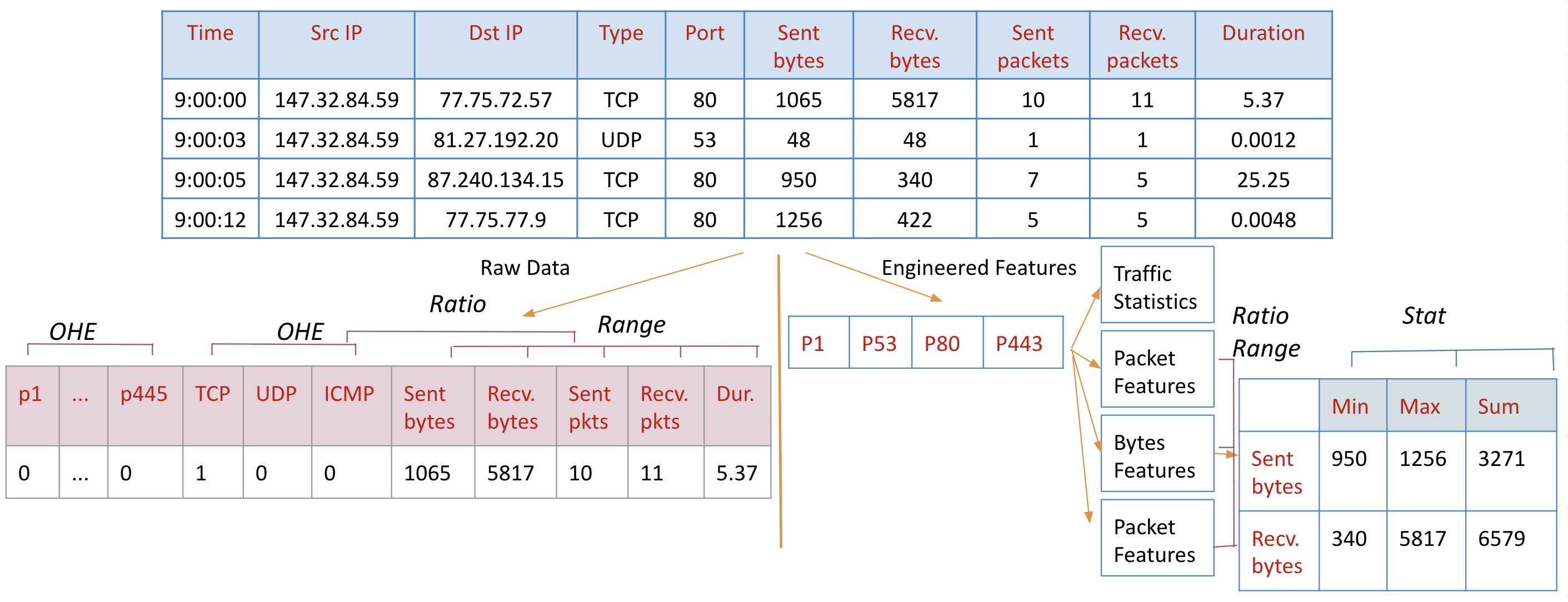
Figure 3. Zeek logs (top), raw data representation (left), and feature families per port (right) for network traffic classifier.

In this application, we can use either the raw connection representation or leverage domain knowledge to create aggregated features. We describe existing feature relationships and apply our FENCE framework against both representations.

Raw Data Representation. This consists of the following fields: one-hot encoded port number, one-hot encoded connection type, duration, original bytes, received bytes, original packets, and received packets. The feature vector is illustrated in Figure 3 on the left. The raw data representation includes no mathematical dependencies, but has the following domain-specific constraints:

- The TCP and UDP packet sizes are capped at 1500 bytes. We create range intervals for these values, resulting in a $Ratio$ dependency between the number of packets and their sizes.

- The connection duration is the interval between the last and the first packet. If the connection is idle for some time interval (e.g., 30 seconds), it is closed by default by Zeek. The attacker can thus control the duration of the connection by sending packets at certain time intervals to avoid closing the connection. We generate a range of valid durations from the distribution of connection duration in the training dataset. This creates again a $Ratio$ dependency between the number of packets and their duration.

- Each continuous feature has its related minimum and maximum values, which are obtained from the training data distribution, thus forming $Range$ relationships.

- The port number and connection type have one-hot encoded $OHE$ dependencies.

Attack algorithm on raw data representation. The attacker’s goal is to have a connection log classified as $\mathsf{Benign}$ instead of $\mathsf{Malicious}$. We assume that the attacker communicates with an external IP under its control (for instance, the command-and-control IP), and thus has full control of the malicious traffic in that connection. We assume that the attacker can only add traffic to network connections, by increasing the number of bytes, packets, and connection duration, to preserve the malicious functionality. For simplicity, we set the number of received packets and bytes to 0, assuming that the external IP does not respond to these connections. We assume that the attacker does not have access to the security monitor that collects the logs and cannot modify directly the log data.

The attack algorithm follows the framework from Algorithm 1. There is only one family of dependent features, including the packets and bytes sent, and connection duration. The representative feature is the number of sent packets, which is updated with the gradient value, following a binary search for perturbation $\delta$, as specified in Algorithm $\mathsf{UPDATE\_FAMILY}$. The dependent number of bytes sent and duration features are updated using the update dependency functions ($\mathsf{Update\_Ratio}$, Update_Range and Update_OHE), thus preserving the $Ratio$, $Range$ and $OHE$ dependencies.

Engineered Features. Another possibility is to use domain knowledge to create features that improve classification accuracy. A standard method for creating network traffic features is aggregation by destination port to capture relevant traffic statistics per port (e.g., (Garcia et al., 2014), (Ongun et al., 2019)). This is motivated by the fact that different network services and protocols run on different ports, and we expect ports to have different traffic patterns. We select a list of 17 ports for popular applications, including HTTP (80), SSH (22), and DNS (53). We also add a category called OTHER for connections on other ports. We aggregate the communication on a port based on a fixed time window (the length of which is a hyper-parameter set at one minute). For each port, we compute traffic statistics using the $\mathsf{Max}$, $\mathsf{Min}$, and $\mathsf{Total}$ operators for outgoing and incoming connections. See the example in Figure 3 on the right, in which features extracted for each port define a family of dependent features. We obtain a total of 756 aggregated traffic features on these 17 ports. Table 5 includes the feature description. The resulting feature vector includes both types of dependencies. The domain-specific relationships are the same as for the raw data representation except for the one-hot encoding relationship. There are additional $Stat$ mathematical dependencies between features: the minimum and the maximum number of packets, bytes and duration per connection must be updated after a change in the total number of packets, bytes, or connections.

Category	Feature	Description
Bytes	Total_Sent_Bytes	Total number of bytes sent
	Min_Sent_Bytes	Minimum number of bytes sent per connection
	Max_Sent_bytes	Maximum of bytes sent per connection
Packets	Total_Sent_Pkts	Total number of packets sent
	Min_Sent_Pkts	Minimum number of packets sent per connection
	Max_Sent_Pkts	Maximum of packets sent per connection
Duration	Total_Duration	Total duration of all connections
	Min_Duration	Minimum duration of a connection
	Max_Duration	Maximum duration of a connection
Connection type	Total_TCP	Total number of TCP connections
	Total_UDP	Total number of UDP connections

Table 5. Features definition for malicious connection classification. These features are defined for each port by aggregating over all connections on that port in a fixed time window.

Attack algorithm on engineered features. The goal of the attacker here is to change the prediction of a feature vector aggregated over time from $\mathsf{Benign}$ to $\mathsf{Malicious}$. Therefore, in this attack model, the attacker has the ability to insert network connections during the targeted time window to achieve his goal. Similar to the above scenario, the attacker controls a victim IP and can send traffic to external IPs under its control. The adversary has a lot of options in mounting the attack by selecting the protocol, port, and connection features. Here we have 17 families of dependent features, one for the features on each port.

The attack algorithm against the Neris botnet classification task called the Neris attack follows the framework from Algorithm 1. First, the feature of the maximum gradient is determined and the corresponding port is identified. The family of dependent features is all the features computed for that port. The attacker attempts to add a fixed number of connections on that port (which is a hyper-parameter of our system). This is done in the $\mathsf{INIT\_FAMILY}$ function. The attacker can add either TCP, UDP, or both types of connections, according to the gradient sign for these features and also respecting network-level constraints. The representative feature for a port’s family is the number of packets that the attacker sends in a connection. This feature is updated by the gradient value, following a binary search for perturbation $\delta$, as specified in Algorithm $\mathsf{UPDATE\_FAMILY}$ .

In the $\mathsf{UPDATE\_DEP}$ function an update to the aggregated port features is performed. First, we ensure that the feature corresponding to the number of packets sent satisfies the $Range$ and $Stat$ constraints. Then the difference in the total number of bytes sent by the attacker and duration is determined from the gradient, followed by the $\mathsf{Update\_Ratio}$ function to keep the resulting values inside the feasible domain. The port family also includes features such as $\mathsf{Min}$ and $\mathsf{Max}$ sent bytes and connection duration. These features are updated by the $\mathsf{Update\_Stat}$ function. The detailed algorithm for $\mathsf{INIT\_FAMILY}$ and $\mathsf{UPDATE\_DEP}$ functions of the Neris attack are illustrated in Algorithm 7 and Algorithm 8.

Algorithm 7 Neris $\mathsf{INIT\_FAMILY}$ ($x^{m},\nabla,j$)

0:  $x^{m}$: data point in iteration $m$$\nabla$: gradient of objective with respect to $x$ $j$: representative feature of the the family$p$: port updated in iteration $m$$c$: number of connections to add

1:  // Check if the connections are allowed on port $p$

2:  $ac\leftarrow$ ALLOWED_CONNECTIONS$(p,x^{m})$

3:  if $\nabla_{c}<0$ and $ac==True$ then

4:     return  $c$

5:  end if

6:  return  0

Algorithm 8 Neris $\mathsf{UPDATE\_DEP}$ ($s,x^{m},\nabla,F_{i_{max}}$)

0:  $s$: number of added connections$x^{m}$: data point in iteration $m$$F_{i_{max}}$: all dependent features on the feature of maximum gradient $i_{max}$ $x^{\mathsf{tot}}_{\mathsf{packets}}$/$x^{\mathsf{min}}_{\mathsf{packets}}$/$x^{\mathsf{max}}_{\mathsf{packets}}$: total/min/max number of sent packets on $p$ per connection$x^{\mathsf{tot}}_{\mathsf{bytes}}$/$x^{\mathsf{min}}_{\mathsf{bytes}}$/$x^{\mathsf{max}}_{\mathsf{bytes}}$: total/min/max number of sent bytes on $p$ per connection$x^{\mathsf{tot}}_{\mathsf{dur}}$/$x^{\mathsf{min}}_{\mathsf{dur}}$/$x^{\mathsf{max}}_{\mathsf{dur}}$: total/min/max duration on $p$ per connection$\nabla$: gradient of objective with respect to $x$ $minP$: the minimum total number of sent packets from data distrinution$maxP$: the maximum total number of sent packets from data distribution$minB$: the minimum total number of sent bytes from data distrinution$maxB$: the maximum total number of sent bytes from data distribution$minD$: the minimum total connections duration from data distribution$maxD$: the maximum total connections duration from data distribution

1:  $x^{\mathsf{tot}}_{\mathsf{packets}},\Delta^{\mathsf{tot}}_{\mathsf{packets}}\leftarrow$ Update_Range($x^{m},minP,maxP$)

2:  $x^{\mathsf{min}}_{\mathsf{packets}},x^{\mathsf{max}}_{\mathsf{packets}}\leftarrow\mathsf{Update\_Stat}(x^{m},\Delta^{\mathsf{tot}}_{\mathsf{packets}}/s,F^{\mathsf{packets}}_{i_{max}})$

3:  $x^{\mathsf{tot}}_{\mathsf{bytes}}\leftarrow\mathsf{Update\_Ratio}(x^{m},\nabla^{\mathsf{tot}}_{\mathsf{bytes}},F^{\mathsf{bytes}}_{i_{max}})$

4:  $x^{\mathsf{tot}}_{\mathsf{bytes}},\Delta^{\mathsf{tot}}_{\mathsf{bytes}}\leftarrow$ Update_Range$(x^{\mathsf{tot}}_{\mathsf{bytes}},minB,maxB)$

5:  $x^{\mathsf{min}}_{\mathsf{bytes}},x^{\mathsf{max}}_{\mathsf{bytes}}\leftarrow\mathsf{Update\_Stat}(x^{m},\Delta^{\mathsf{tot}}_{\mathsf{bytes}}/s,F^{\mathsf{bytes}}_{i_{max}})$

6:  $x^{\mathsf{tot}}_{\mathsf{dur}}\leftarrow\mathsf{Update\_Ratio}(x^{m},\nabla^{\mathsf{tot}}_{\mathsf{dur}},F^{\mathsf{dur}}_{i_{max}})$

7:  $x^{\mathsf{tot}}_{\mathsf{dur}},\Delta^{\mathsf{tot}}_{\mathsf{dur}}\leftarrow$ Update_Range $(x^{\mathsf{tot}}_{\mathsf{dur}},minD,maxD)$

8:  $x^{\mathsf{min}}_{\mathsf{dur}},x^{\mathsf{max}}_{\mathsf{dur}}\leftarrow\mathsf{Update\_Stat}(x^{m},\Delta^{\mathsf{tot}}_{\mathsf{dur}}/s,F^{\mathsf{dur}}_{i_{max}})$

4.2. Malicious Domain Classifier

The second threat detection application is to classify FQDN domain names contacted by enterprise hosts as $\mathsf{Malicious}$ or $\mathsf{Benign}$. This security application has multiple types of feature-space constraints, including linear, non-linear, and statistical dependencies, and therefore can be used to test our FENCE framework for supporting multiple constraints.

Dataset. We obtained access to a proprietary dataset collected by a company that includes 89 domain features extracted from HTTP proxy logs collected at the border of an enterprise network. This is the same dataset used for the design of MADE system for detecting malicious activity in enterprise networks and prioritizing the detected activities according to their risk described in detail by Oprea et al. (Oprea et al., 2018). This dataset enables us to experiment with the variety of constraints in feature space, representative of security applications. Features are aggregated over multiple HTTP connections to the same external FQDN domain and are defined with the help of security experts. Each external FQDN is labeled as $\mathsf{Malicious}$ or $\mathsf{Benign}$. We group the modifiable features of MADE into a set of 7 families, included in Table 6. More details on all the features used in MADE are provided in the original paper (Oprea et al., 2018) (we preserved the feature ID for the MADE dataset in Table 6).

In this application, we do not have access to the raw HTTP traffic, only to features extracted from it and domain labels. Thus, the constraints are mathematical constraints in feature space, for instance:

• For the Connection family, we have $NonLin$ dependence: computing average value over a number of events.

• For the Bytes family, we need to update the ratio of two values and then update minimum, maximum and average values, thus, we have the combination of $Stat$ and $NonLin$ dependencies.

• For the HTTP Method, we have the same combination of $Stat$ and $NonLin$ dependencies as for Bytes family.

• For the Content family, we need to ensure that the sum of all ratio values equals 1. This is a combination of $Lin$ and $NonLin$ dependencies.

• For the Result Code, we also need to ensure that the sum of all fraction values equals to 1. Additionally, the number of connections with different codes must sum up to the total number of connections. This is a combination of $Lin$ and $NonLin$ dependencies.

Attack algorithm. We assume that we add events to the logs, and never delete or modify existing events. For instance, we can insert more connections, as in the malicious connection classifier. The attack algorithm against the malicious domain classifier called the MADE attack follows the framework from Algorithm 1. If the feature of the maximum gradient has no dependencies, it is just updated with the gradient value. Otherwise, every dependency family has a specific representative feature and is updated following one of the specified $\mathsf{UPDATE\_DEP}$ functions. For example, for the Connection family, the representative feature is Num_Conn, which is updated with the gradient value, and other features in this family are updated by calling the $\mathsf{Update\_Stat}$ function. The detailed algorithm for the $\mathsf{UPDATE\_DEP}$ function of the MADE attack is illustrated in Algorithm 9. The functions for updating dependencies (e.g., $\mathsf{Update\_Stat}$, $\mathsf{Update\_Lin}$, $\mathsf{Update\_NonLin}$) are the same defined in the FENCE framework and discussed in Section 3.4.

Family	Feature ID	Feature	Description
Connections	1	Num_Conn	Number of established connections
	2	Avg_Conn	Average number of connections per host
Bytes	3	Total_Recv_Bytes	Total number of received bytes
	4	Total_Sent_Bytes	Total number of sent bytes
	5	Avg_Ratio_Bytes	Average ratio of received bytes
			over sent bytes per IP
	6	Min_Ratio_Bytes	Maximum ratio of received bytes
			over sent bytes per IP
	7	Max_Ratio_Bytes	Minimum ratio of received bytes
			over sent bytes per IP
HTTP	8	Num_POST	Total number of POST requests
Method	9	Num_GET	Total number of GET requests
	10	Avg_POST	Average number of POST requests
			over GET requests per IP
	11	Min_POST	Minimum number of POST requests
			over GET requests per IP
	12	Max_POST	Maximum number of POST requests
			over GET requests per IP
Content	46	Frac_empty	Fraction of connections with empty content type
	47	Frac_js	Fraction of connections with js content type
	48	Frac_html	Fraction of connections with html content type
	49	Frac_img	Fraction of connections with image content type
	50	Frac_video	Fraction of connections with video content type
	51	Frac_text	Fraction of connections with text content type
	52	Frac_app	Fraction of connections with app content type
Result	59	Num_200	Number of connections with result code 200
Code	60	Num_300	Number of connections with result code 300
	61	Num_400	Number of connections with result code 400
	62	Num_500	Number of connections with result code 500
	63	Frac_200	Fraction of connections with result code 200
	64	Frac_300	Fraction of connections with result code 300
	65	Frac_400	Fraction of connections with result code 400
	66	Frac_500	Fraction of connections with result code 500
Independent	43	Avg_OS	Average number operating systems
			extracted from user-agent
	44	Avg_Browser	Average number of browsers used
	68	Dom_Levels	Number of levels
	69	Sub_Domains	Number of sub-domains
	70	Dom_Length	Length of domain
	71	Reg_Age	WHOIS registration age
	72	Reg_Validity	WHOIS registration validity
	73	Update_Age	WHOIS update age
	74	Update_Validity	WHOIS update validity
	75	Num_ASNs	Number of ASNs
	76	Num_Countries	Number of countries contacted the domain

Table 6. Feature set for malicious domain classification that can be modified by the evasion attack.

Algorithm 9 MADE $\mathsf{UPDATE\_DEP}$ ($s,x^{m},\nabla,F_{i_{max}}$)

0:  $s$: type of dependency family $x^{m}$: data point in iteration $m$$\nabla$: gradient of objective with respect to $x$ $F_{i_{max}}$: all dependent features on $i_{max}$$i_{max}$: feature of maximum gradient

1:  if $s==\mbox{Stat}$ then

2:     $v\leftarrow$NEW_VALUE_ADDED$(x^{m},\nabla,F_{i_{max}})$

3:     $\mathsf{Update\_Stat}(x^{m},v,F_{i_{max}})$

4:  end if

5:  if $s==\mbox{Lin}$ then

6:     $\mathsf{Update\_Lin}(x^{m},\nabla,F_{i_{max}})$

7:  end if

8:  if $s==\mbox{NonLin}$ then

9:     $\mathsf{Update\_NonLin}(x^{m},\nabla,F_{i_{max}})$

10:  end if

11:  if $s==\mbox{Combination}$ then

12:     $\mathsf{Update\_Comb}(x^{m},\nabla,F_{i_{max}})$

13:  end if

5. Experimental evaluation for network traffic classifier

We evaluate FENCE for the malicious network traffic classifier trained with both the raw data and engineered feature representations. We show feasible attacks that insert a small number of network connections to change the $\mathsf{Malicious}$ prediction to $\mathsf{Benign}$. We only analyze the FENCE attack with the Projected optimization objective here. In the following section, we analyze our FENCE framework for the malicious domain classifier for both the Projected and Penalty attacks.

5.1. Experimental setup

CTU-13 is a collection of 13 scenarios including both legitimate traffic from a university campus network, as well as labeled connections of malicious botnets (Garcia et al., 2014). We restrict to three scenarios for the Neris botnet (1, 2, and 9). We choose to train on two of the scenarios and test the models on the third, to guarantee independence between training and testing data.

The raw data representation has 3,712,935 data points, from which 151,625 are labeled as botnets. The attacker can modify three features per connection: bytes and packets sent, and duration. The training data in the engineered features representation has 3869 $\mathsf{Malicious}$ examples, and 194,259 $\mathsf{Benign}$ examples, and an imbalance ratio of 1:50. There is a set of 432 statistical features that the attacker can modify (the ones that correspond to the characteristics of sent traffic on 17 ports). The physical constraints and statistical dependencies in both scenarios have been detailed in Section 4.1.

We considered two baseline attacks: Baseline 1 (in which the features that are modified iteratively are selected at random), and Baseline 2 (in which, additionally, the amount of perturbation is sampled from a standard normal distribution $N(0,1)$).

5.2. Attack results for raw data representation

For training we have used FFNN with two layers and a sigmoid activation function. The architecture that corresponds to the best performance has 12 neurons in the first layer, and 1 neuron in the second layer. We have trained it using Adam optimizer with a learning rate equal to 0.0001 for 20 epochs with batch size 64. The best results are for training on scenarios 2 and 9, and testing on scenario 1, with an F1 score of 0.70.

We consider an attack on testing scenario 1, and the success rate of our attack is 100% already at a small $L_{2}$ distance of 2. Intuitively, an attacker can add a few packets and bytes to a connection and change its classification easily. We compare its performance to Baseline 2, which achieves only 73% success rate at $L_{2}$ distance of 2.

5.3. Attack results for engineered features

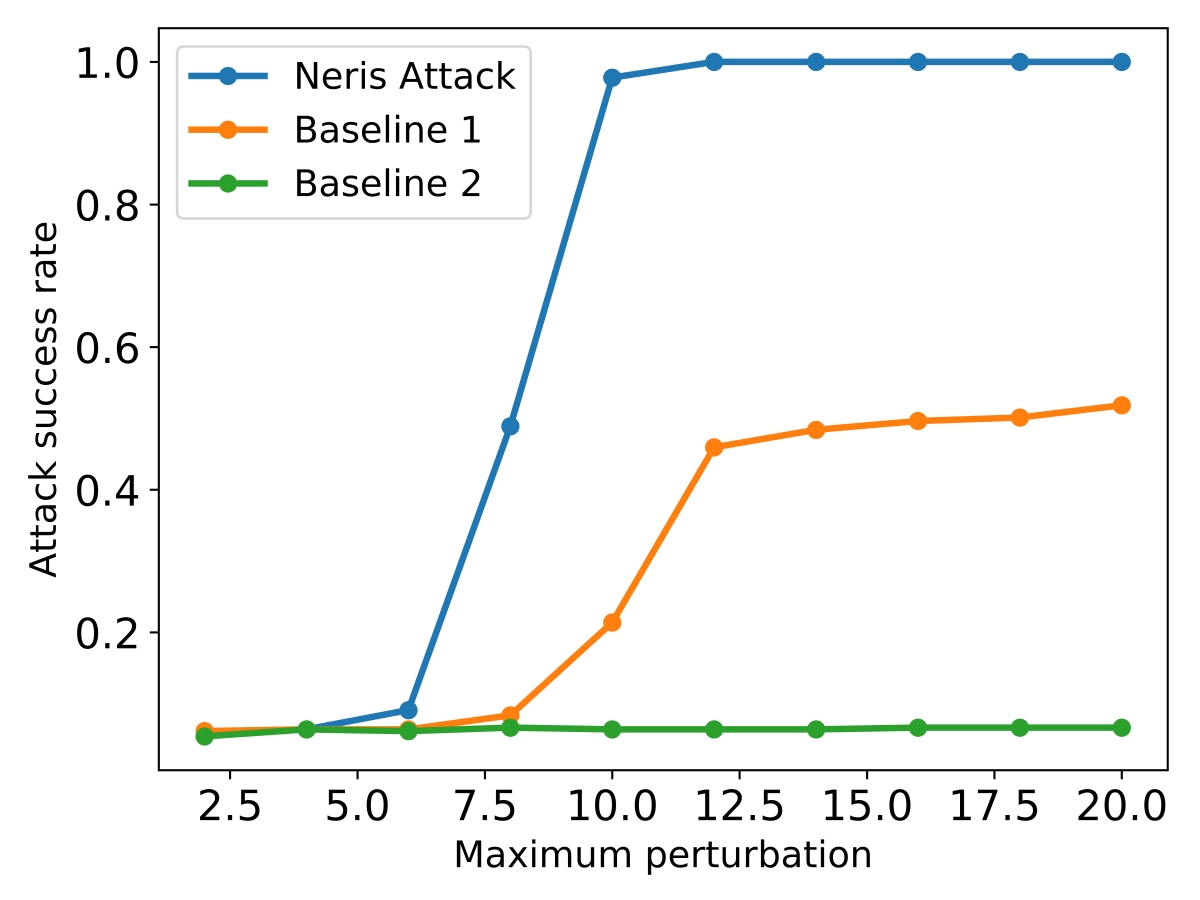
(a) FENCE Projected attack
success rate.

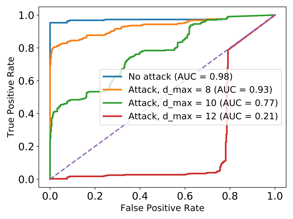
(b) ROC curves under FENCE
Projected attack.

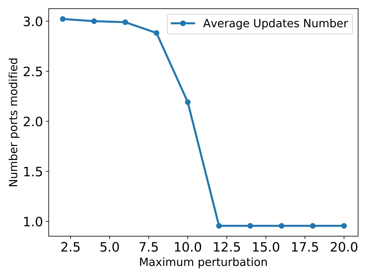
(c) Average number of updated
ports.

Figure 4. Projected attack results on network traffic classifier.

We perform model selection and training for a number of FFNN architectures on all combinations of two scenarios, and tested the models for generality on the third scenario. The best architecture consists of three layers with 256, 128 and 64 hidden layers. We used the Adam optimizer, 50 epochs for training, a mini-batch of 64, and a learning rate of 0.00026. The F1 and AUC scores are much better than the FFNN based on raw data representation. For instance, the best scenario is training on 1, 9, and testing on 2, which achieve an F1 score of 0.97, compared to 0.70 for raw data.

We thus perform a more extensive analysis of the attack against engineered features in this scenario. The testing data for the attack is 407 $\mathsf{Malicious}$ examples from scenario 2, among which 397 were predicted correctly by the classifier.

Evasion attack performance. First, we analyze the attack success rate with respect to the allowed perturbation, shown in Figure 4(a). The attack reaches 99% success rate at $L_{2}$ distance 16. Interestingly, in this case the two baselines perform poorly, demonstrating again the clear advantages of our framework. We plot next the ROC curves under evasion attack in Figure 4(b) (using the 407 $\mathsf{Malicious}$ examples and 407 $\mathsf{Benign}$ examples from testing scenario 2). At distance 8, the AUC score is 0.93 (compared to 0.98 without adversarial examples), but there is a sudden change at distance 10, with the AUC score dropping to 0.77. Moreover, at distance 12, the AUC reaches 0.12, showing the model’s degradation under evasion attack with relatively small distance.

ts	port	prot	duration	o_bts	r_bts	o_pkts	r_pkts	state
1	53	UDP	2.26638	67	558	2	2	SF
2	13363	TCP	444.334	707	671	14	11	SF
3	1035	TCP	276.084218	20768	0	110	0	OTH
4	443	TCP	432.47	112404	0	87	0	OTH

Table 7. Example of Zeek logs records (top 3 rows), and one of the 12 attacker-generated connection logs added for the adversarial example perturbation (4th row).

Feature	Average	Std. Dev.	25 %	50 %	75 %	95 %	Maximum
Duration	552.20	7872.84	0.13	5.71	79.38	1578.82	1060383.73
Orig_Bytes	150756.59	12976082.76	96	415	2466	51117.3	2091734081
Orig_Pkts	342.75	5221.95	2	9	34	522	405463

Table 8. Feature statistics in training data.

Setting	Average	Std. Dev.	25 %	50 %	75 %	95 %	Maximum
Training data	38.12	98.85	2.42	4.52	24.53	195.58	890.56
Projected perturbation	7.66	0.57	7.66	7.85	7.93	7.97	7.99

Table 9. $L_{2}$ norm statistics for training data (top row) and perturbation added by the Projected attack (bottom row).

The average number of port families updated during the attack is shown in Figure 4(c). The maximum number is 3 ports, but it decreases to 1 port at distance higher than 12. While counter-intuitive, at larger distances the attacker can add larger perturbation to the aggregated statistics of one port, crossing the decision boundary. The ports most frequently modified are 443 and 80, which are the ports with most network traffic.

Adversarial examples. We show an adversarial example generated by the Projected attack at distance 14. The attacker adds only 12 TCP connections on port 443, including 87 packets, each of size 1292 bytes, with connection duration of 432.47 seconds. Table 7 shows one of the 12 attacker-generated connections to create the adversarial example. The destination IP can be selected by the attacker so that it is under its control and does not send any bytes or packets. These new connections are added to the activity the attacker already does inside the network, so the malicious functionality of the attack is preserved. Interestingly, all adversarial attacks succeed with at most 12 new connections at distances higher than 10. In Table 8 we show statistics for the duration, sent bytes and sent packets features in the training data. We make the observation that the feature values in the resulting adversarial example are below the average feature values of the training data. In particular, the Orig_Bytes feature has an average value 150KB and a very high standard deviation (12.9MB), while the adversarial example only uses 112,404 bytes, which is very little communication (112KB).

Furthermore, we illustrate the $L_{2}$ norm statistics of samples in the training data along with $L_{2}$ norms of perturbations added to create adversarial examples at distance 8 in Table 9. We observe that the average $L_{2}$ perturbation norm (7.66) is 4.97 times lower than the training data average $L_{2}$ norm (38.12). Given that the standard deviation (0.57) and maximum value (7.99) of the perturbation $L_{2}$ norm are small compared to the standard deviation (98.85) and the maximum value (890.56) of the $L_{2}$ norm of training samples, we consider the resulting adversarial attacks stealthy.

6. Experimental evaluation for malicious domain classifier

In this section we perform a detailed evaluation of the FENCE attack on the MADE malicious domain classifier trained on the enterprise dataset (Oprea et al., 2018). We compare the Projected and Penalty optimization methods and analyze the impact of imbalanced training datasets. We also test the transferability of the FENCE attacks across other models and architectures and evaluate the potential of adversarial training as mitigation against FENCE evasion attacks.

6.1. Experimental setup

The data for training and testing the models was extracted from security logs collected by web proxies at the border of a large enterprise network with over 100,000 hosts. The number of monitored external domains in the training set is 227,033, among which 1730 are classified as $\mathsf{Malicious}$ and 225,303 are $\mathsf{Benign}$. For training, we sampled a subset of training data to include 1230 $\mathsf{Malicious}$ domains, and a different number of $\mathsf{Benign}$ domains to get several imbalance ratios between the two classes (1, 5, 15, 25, and 50). We used the remaining 500 $\mathsf{Malicious}$ domains and sampled 500 $\mathsf{Benign}$ domains for testing the evasion attack. Overall, the dataset includes 89 features from 7 categories.

Among the features included in the dataset, we determined a set of 31 features that can be modified by an attacker (see Table 6 for their description). These include communication-related features (e.g., number of connections, number of bytes sent and received, etc.), as well as some independent features (e.g., number of levels in the domain or domain registration age). Other features in the dataset (for example, those using URL parameters or values) are more difficult to change, and we consider them immutable during the evasion attack.

This dataset is extremely imbalanced, and we sample a different number of $\mathsf{Benign}$ domains from the data, to control the imbalance ratio. We are interested in how the imbalance affects the attack success rate. On this dataset, we also compare the Projected and Penalty attack objectives.

6.2. FENCE attack evaluation

We experimented with several models for training classifiers, including logistic regression, random forest, and different FFNN architectures. The best performance was achieved by a two-layer FFNN with 80 neurons in the first layer, and 50 neurons in the second layer. ReLU activation function is used after all hidden layers except for the last layer, which uses sigmoid. We used the Adam optimizer and SGD with different learning rates. The best results were obtained with Adam and a learning rate of 0.0003. We trained for 75 epochs with a mini-batch size of 32. The resulting model had an AUC score of 89% with cross-validation, in the balanced case. These results were comparable to the best random forest model we trained and better than logistic regression.

The ROC curves for training logistic regression, random forest and FFNN are given in Figure 5 (a), while the results for FFNN with different imbalanced ratios are in Figure 5 (b). Interestingly, the performance of the model increases to 93% AUC for an imbalance ratio up to 25, after which it starts to decrease (with AUC of 83% at a ratio of 50). Our intuition is that the FFNN model achieves better performance when more training data is available (up to a ratio of 25). But once the $\mathsf{Benign}$ class dominates the $\mathsf{Malicious}$ one (at ratio of 50), the model performance starts to degrade.

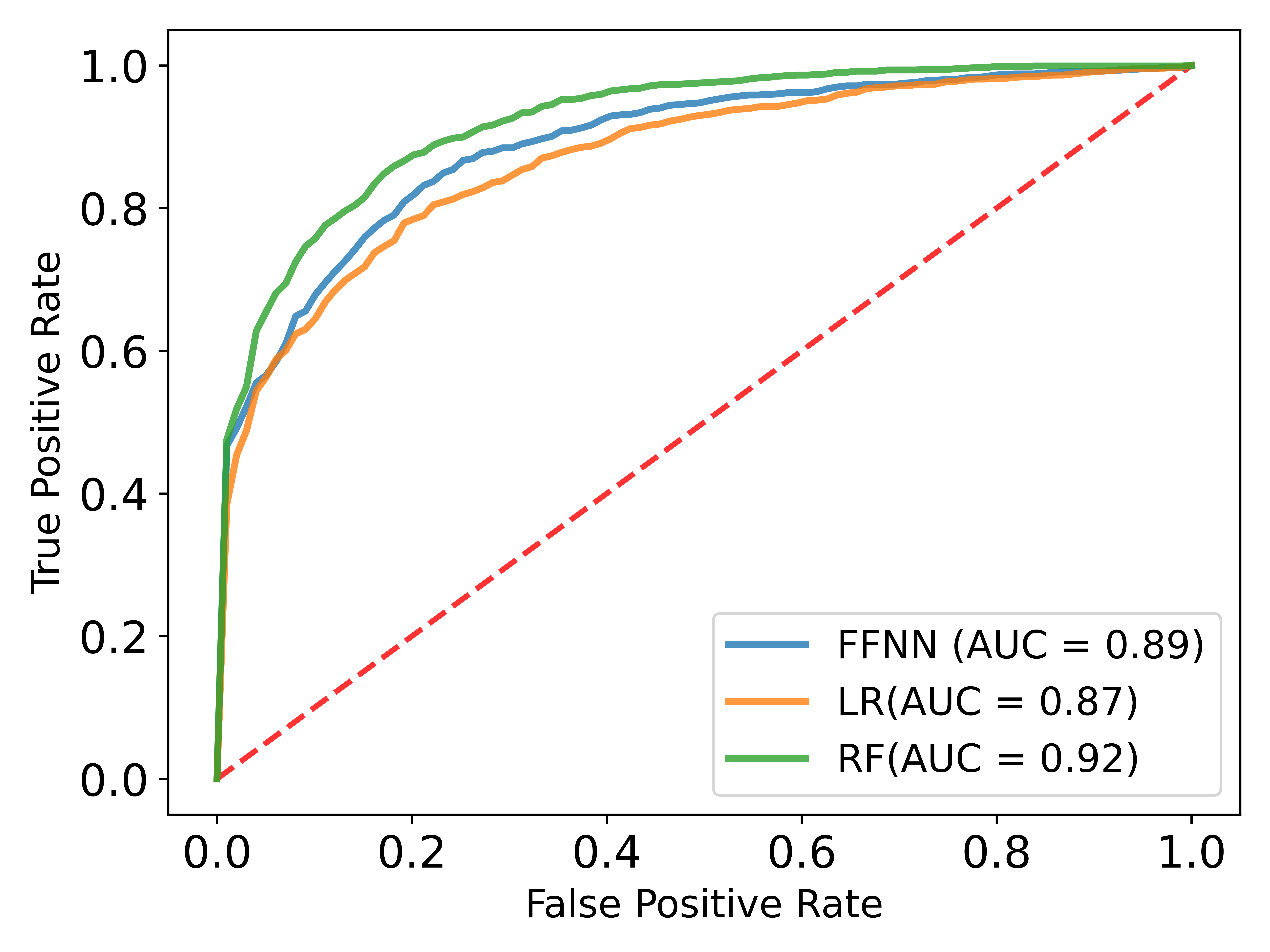
(a) Models performance.

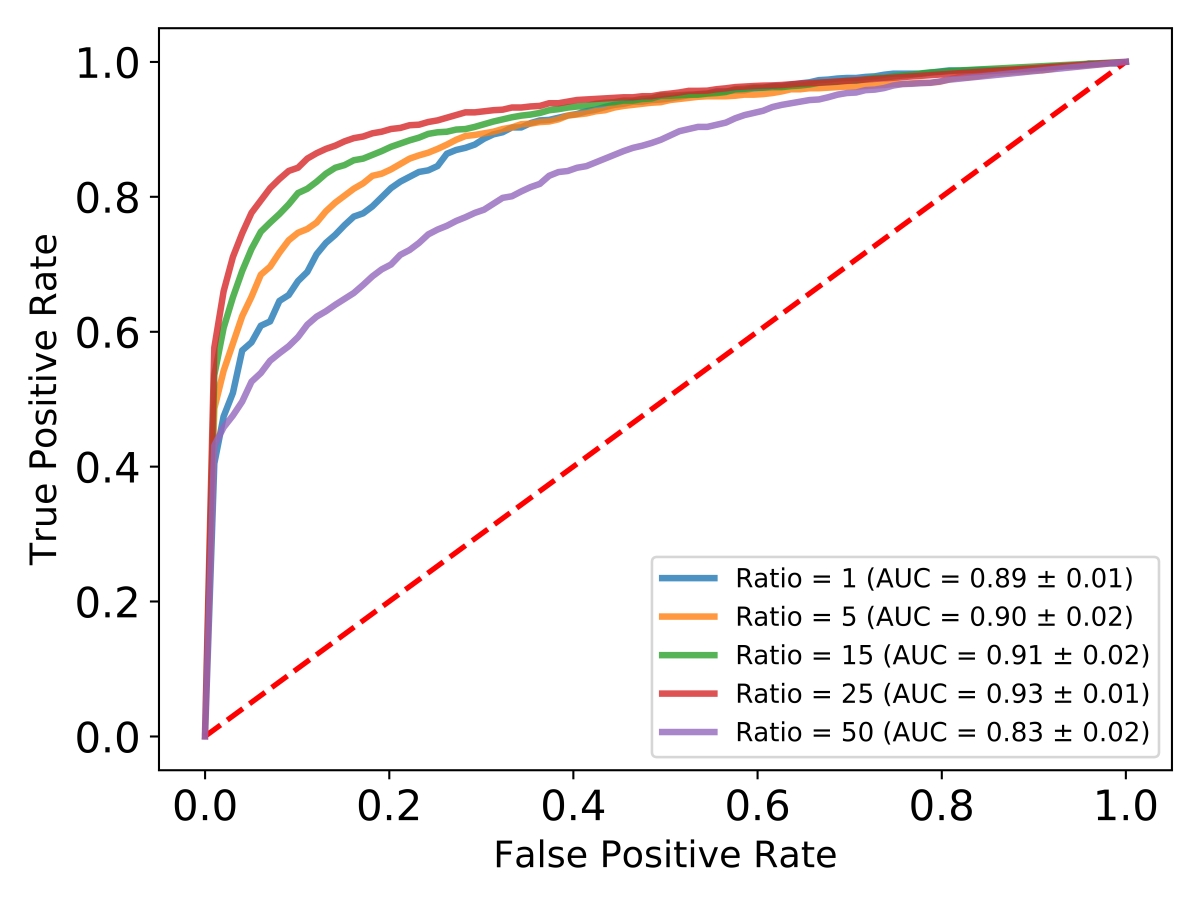
(b) Imbalance results on FFNN.

Figure 5. Training results for malicious domain classifier.

FENCE Projected attack results. We evaluate the success rate of the attack with Projected objective first for balanced classes (1:1 ratio). We compare in Figure 6(a) the attack against the two baselines. The attacks are run on 412 $\mathsf{Malicious}$ testing examples classified correctly by the FFNN. The Projected attack improves both baselines, with Baseline 2 performing much worse, reaching success rate of 57% at a distance of 20, and Baseline 1 has a success of 91.7% compared to our attack (98.3% success). This shows that the attacks are still performing reasonably if feature selection is done randomly, but it is very important to add perturbation to features consistent with the optimization objective.

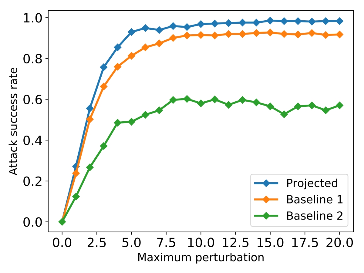
(a) FENCE attack success rate.

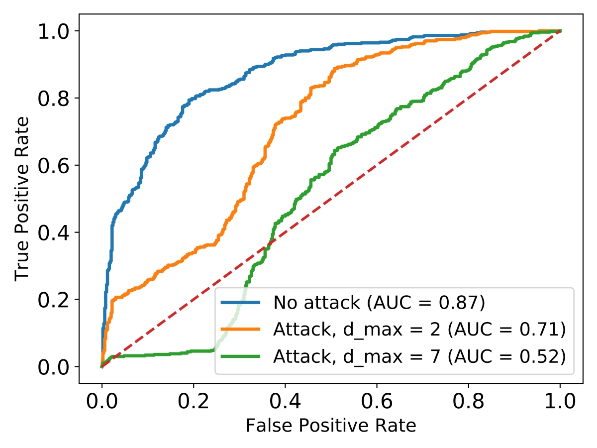
(b) ROC curves under attack.

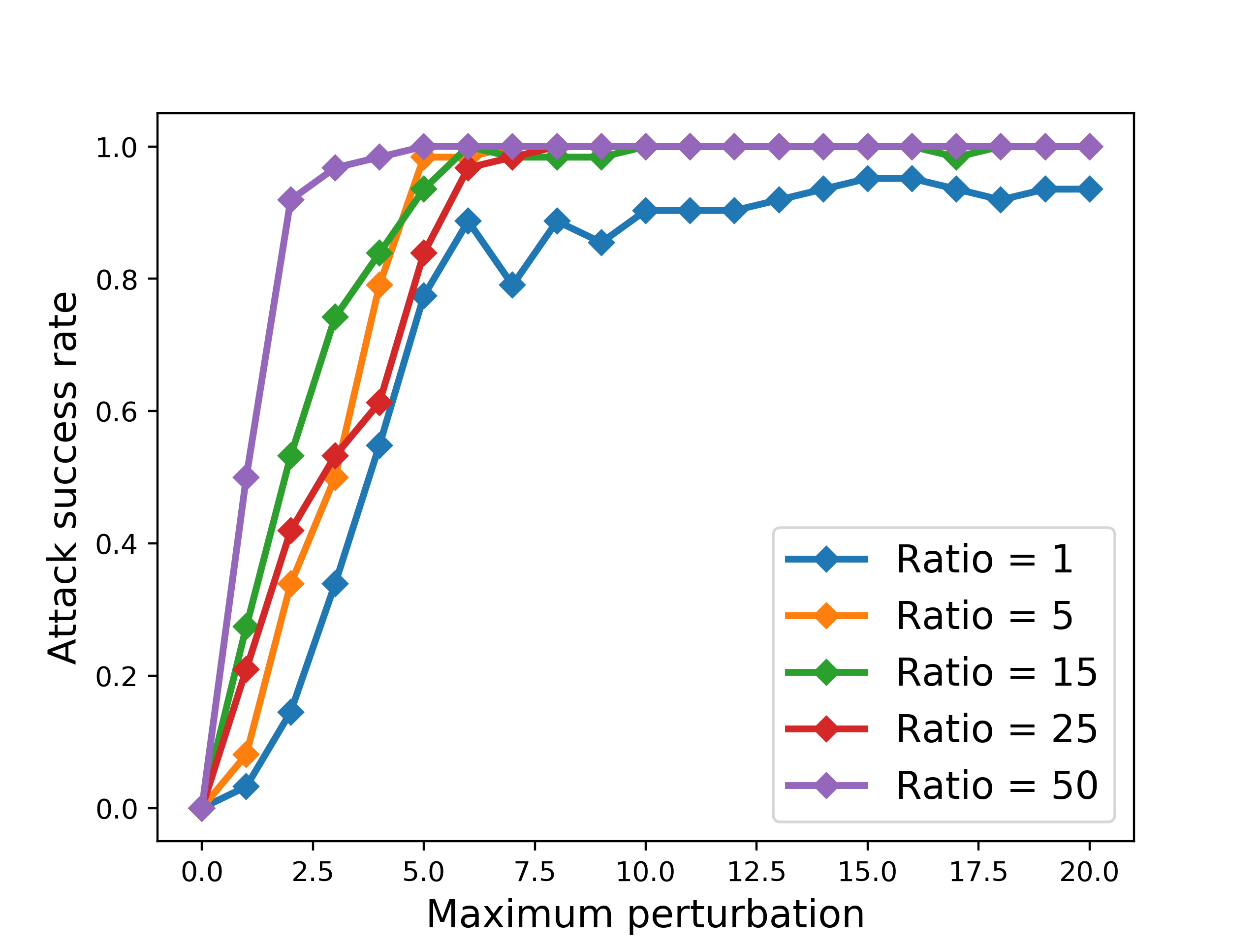
(c) Imbalance sensitivity.

Figure 6. FENCE Projected attack results for the malicious domain classifier.

We also measure in Figure 6(b) the decrease in the model’s performance before and after the evasion attack at different perturbations (using 500 $\mathsf{Malicious}$ and 500 $\mathsf{Benign}$ examples not used in training). While the AUC score is 0.87 originally, it drastically decreases to 0.52 under evasion attack at perturbation 7. This shows the significant degradation of the model’s performance under evasion attack.

Finally, we run the attack at different imbalance ratios and measure its success for different perturbations. In this experiment, we select 62 test examples that all models (trained for different imbalance ratios) classified correctly before the evasion attack. The results are illustrated in Figure 6(c). At $L_{2}$ distance 20, the evasion attack achieves a 100% success rate for all ratios except 1. Additionally, we observe that with a higher imbalance, it is easier for the attacker to find adversarial examples (at a fixed distance). One reason is that models that have lower performance (such as the model trained with 1:50) are easier to attack. Second, we believe that as the imbalance gets higher the model becomes more biased towards the majority class ($\mathsf{Benign}$), which is the target class of the attacker, making it easier to cross the decision boundary between classes.

We include an adversarial example in Table 10. We only show the features that are modified by the attack and their original value. As we observe, the attack preserves the feature dependencies: the average ratio of received bytes over sent bytes (Avg_Ratio_Bytes) is consistent with the number of received (Total_Recv_Bytes) and sent (Total_Sent_Bytes) bytes. In addition, the attack modifies the domain registration age, an independent feature, relevant to malicious domain classification (Ma et al., 2009). However, there is a higher cost to change this feature: the attacker should register a malicious domain and wait to get a larger registration age. If this cost is prohibitive, we can easily modify our framework to make this feature immutable.

Feature	Original	Adversarial
NIP	1	1
Total_Recv_Bytes	32.32	43653.50
Total_Sent_Bytes	2.0	2702.62
Avg_Ratio_Bytes	16.15	16.15
Registration_Age	349	3616

Table 10. Adversarial example for the FENCE Projected attack at distance 10.

We constructed 45 adversarial examples at $L_{2}$ distance 20 and calculated the average perturbation for every feature that was modified to show that the adversarial examples generated at this distance are unnoticeable. The results can be found in Table 11. Additionally, we include statistics for the features on the training dataset in Table 12. We observe that the generated adversarial examples have stealthy perturbations, given the feature distribution and meaning. For example, the number of sent bytes is increased by 17195.3 (17.19KB), the registration age of a domain is increased on average by 1.14 days, while the number of sub domains is increased by 0.28 on average.Moreover, all average perturbations are much smaller than the standard deviation of features in the training data. For instance, the average perturbation of the sub domains number is 0.28 compared to the corresponding standard deviation of 2867.53 in the training data. This additionally confirms the fact that the generated perturbations for adversarial examples can be considered unnoticeable.

Finally, we show the $L_{2}$ norm statistics of samples in the training data along with the $L_{2}$ norm of perturbations added to create adversarial examples by the Projected attack at distance 5 in the first two rows of Table 13. Even if we used a distance of 5 in the Projected attack, many of the generated perturbations have lower norm (in particular, half of the adversarial examples at distance 5 have norm lower than 3.17). The average $L_{2}$ norm of perturbation (3.20) is much smaller than the standard deviation of the training samples $L_{2}$ norm (26.9), resulting in relatively stealthy perturbations. Additionally, the maximum $L_{2}$ norm of perturbation (5) is only a 0.005 fraction of the maximum possible $L_{2}$ norm of the training samples (890).

Feature	Average perturbation
Total_Recv_Bytes	96340
Total_Sent_Bytes	17195.3
Min_Ratio_Bytes	23.26
Sub_Domains	0.28
Reg_Age	1.14
Reg_Validity	158.91
Update_Age	24.98
Update_Validity	59.53

Table 11. Average modified features perturbation for the FENCE Projected attack at distance 20.

Feature	Average	Std. Dev.	25 %	50 %	75 %	95 %	Maximum
Total_Recv_Bytes	3332.4	84148.49	96.09	433.17	1420.07	7092.40	24854191.98
Total_Sent_Bytes	213.76	52373.22	6.16	14.54	31.48	120.46	25133008.74
Min_Ratio_Bytes	94.56	3298.47	2.43	17.58	48.42	181.73	1190540.7
Num_GET	77.22	1704.09	12	30	62	198	746776
Sub_Domains	485.66	2867.53	1	1	2	1247	54632
Reg_Age	2377.44	1880.03	820	2404	3179	6134	16649
Reg_Validity	2914.57	2158.44	1096	2927	4017	6940	37114
Update_Age	348.68	486.29	96	295	385	1128	42215
Update_Validity	839.28	888.90	365	605	908	2928	43587

Table 12. Feature statistics in training data.

Setting	Average	Std. Dev.	25 %	50 %	75 %	95 %	Maximum
Training data	5.79	26.9	3.89	4.52	5.63	10.4	890
Projected perturbation	3.20	1.20	2.17	3.17	4.21	4.99	5
Penalty perturbation	2.76	1.03	1.92	2.56	3.70	4.44	4.92

Table 13. $L_{2}$ norm statistics for feature vectors in training data (first row), perturbation added by the Projected attack (second row, 89% success rate), and perturbation for the Penalty attack (third row, 70% success rate) at distance 5.

FENCE Penalty attack results. We now discuss the results achieved by applying our attack with the Penalty objective on the testing examples. Similar to the Projected attack, we compare the success rate of the Penalty attack to the two types of baseline attacks for balanced classes, in Figure 7(a) (using the 412 $\mathsf{Malicious}$ testing examples classified correctly). Overall, the Penalty objective is performing worse than the Projected one, reaching 79% success rate at $L_{2}$ distance of 20. We observe that in this case both baselines perform worse, and the attack improves upon both baselines significantly. The decrease of the model’s performance under the Penalty attack is illustrated in Figure 7(b) (for 500 $\mathsf{Malicious}$ and 500 $\mathsf{Benign}$ testing examples). While AUC is 0.87 originally on the testing dataset, it decreases to 0.59 under the evasion attacks at the maximum allowed perturbation of 7. Furthermore, we measure the attack success rate at different imbalance ratios in Figure 7(c) (using the 62 testing examples classified correctly by all models). For each ratio value we searched for the best hyper-parameter $c$ between 0 and 1 with step 0.05. Here, as with the Projected attack, we see the same trend: as the imbalance ratio gets higher, the attack performs better, and it works best at imbalance ratio of 50.

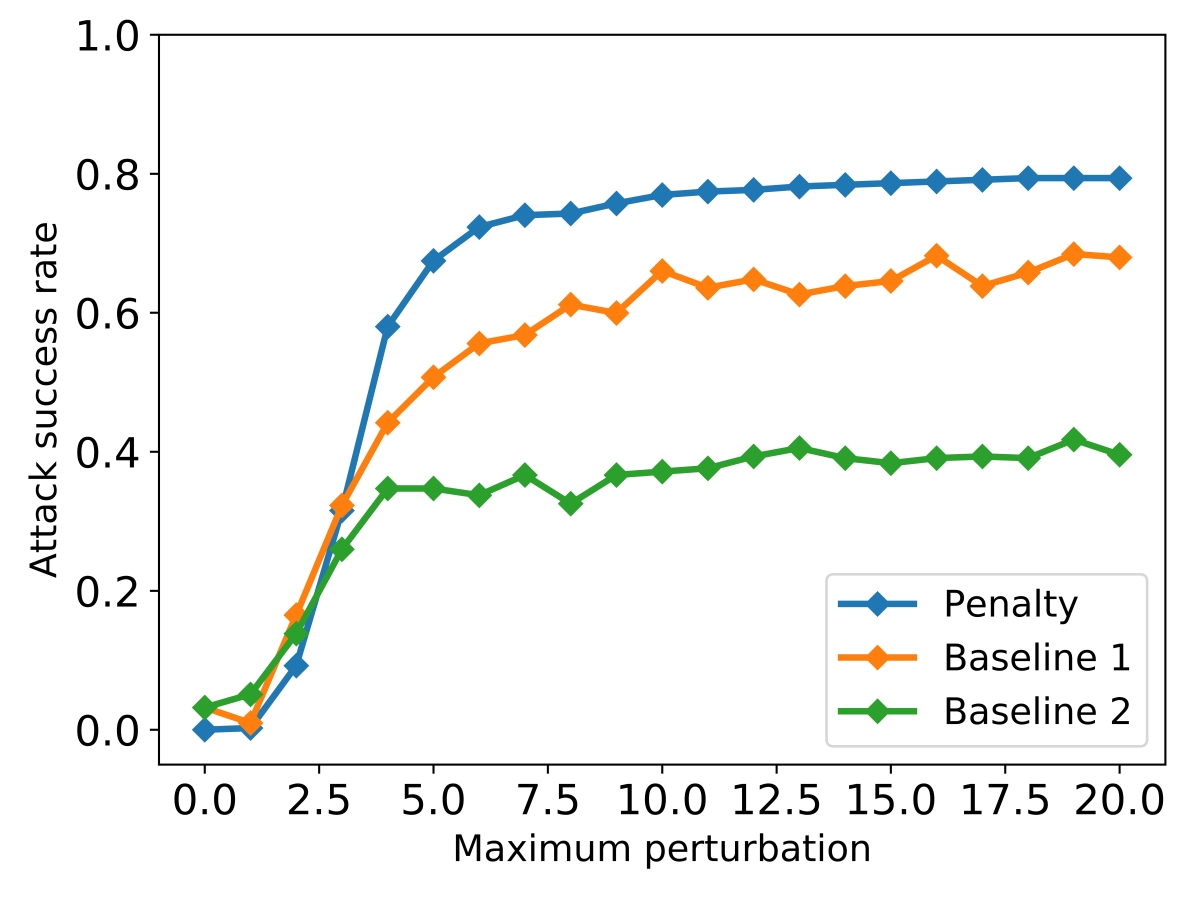
(a) FENCE attack success rate.

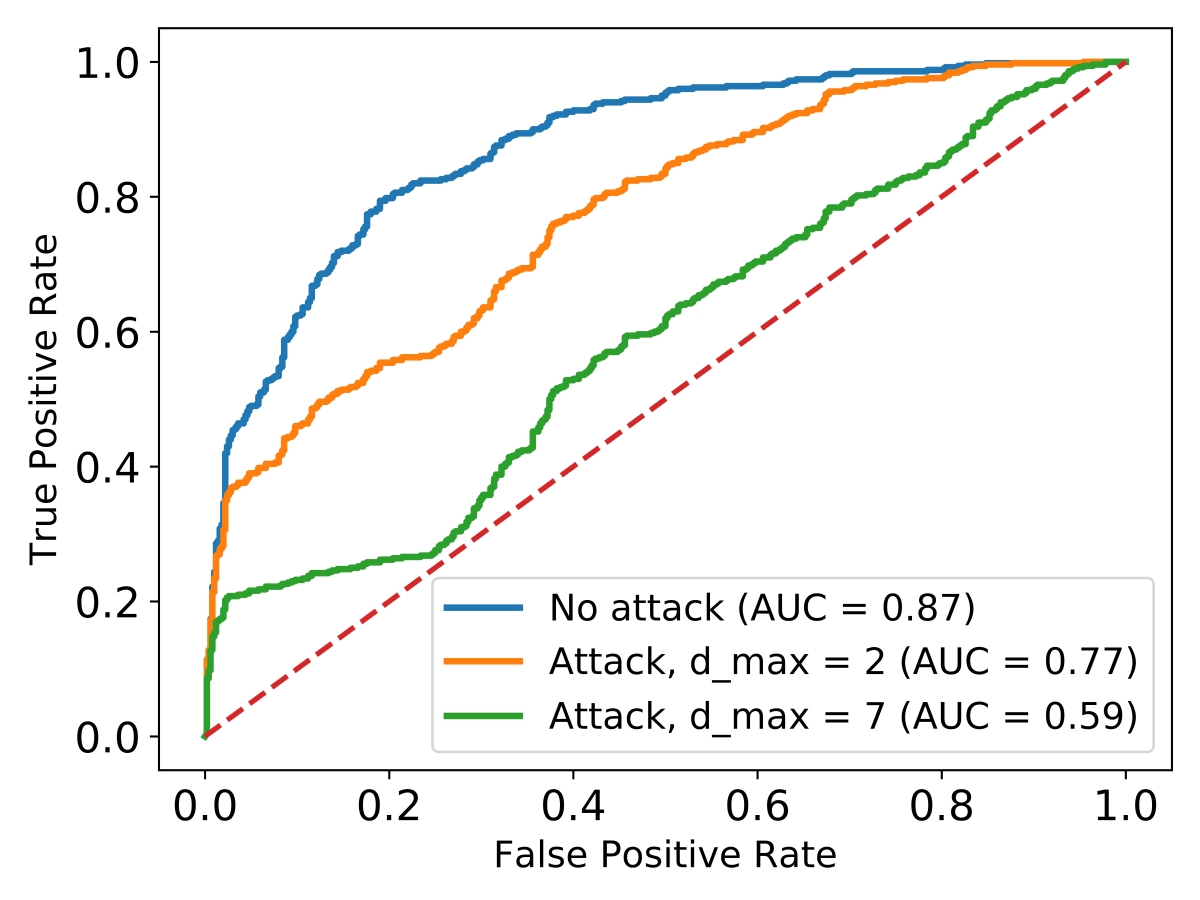
(b) ROC curves under attack.

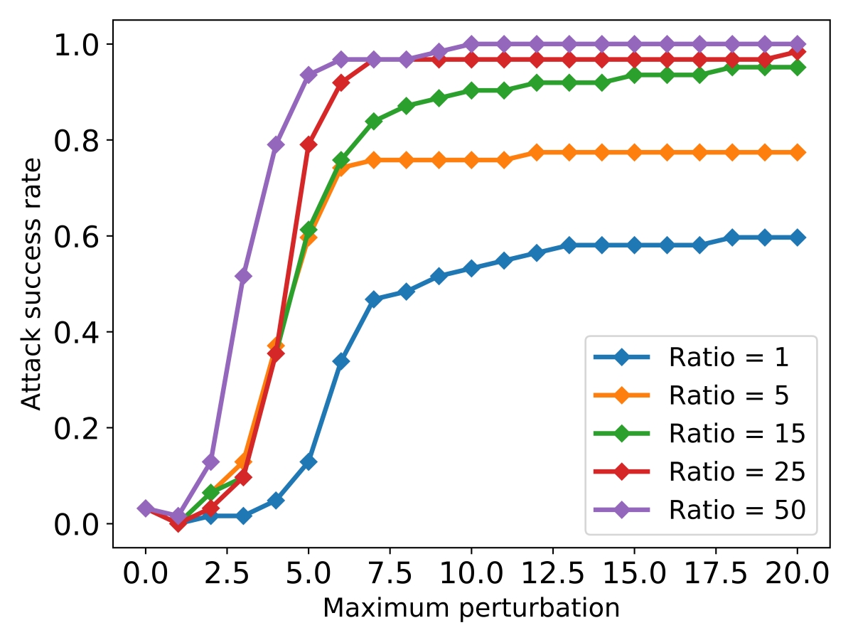
(c) Imbalance sensitivity.

Figure 7. FENCE Penalty attack results for malicious domain classifier.

We include an adversarial example generated by the Penalty attack in Table 14. We only show the features that were updated by the attack, which modifies only the amount of bytes sent (by 4.7KB) and the bytes received (by 73KB). The attack is able to preserve the $Ratio$ dependency: Avg_Ratio_Bytes = Total_Recv_Bytes/Total_Sent_Bytes/NIP.

Feature	Original	Adversarial
NIP	1	1
Total_Recv_Bytes	146.77	73016.06
Total_Sent_Bytes	9.55	4752.92
Avg_Ratio_Bytes	15.36	15.36

Table 14. Adversarial example for the FENCE Penalty attack at distance 10.

We constructed 45 adversarial examples at $L_{2}$ distance 20 for the Penalty attack and calculated the average perturbation for every modified feature. The results are illustrated in Table 15. Given the meaning of the features, we can conclude that an $L_{2}$ distance of 20 can be considered reasonable to generate undetectable attacks. For instance: the Num_GET feature is increased only by 2.19 on average, meaning that the attacker needs to add only 2 or 3 additional GET requests to the domain; the number of sub domains is increased by 0.21; the registration age of the domain is increased by 1.23 days, and the update age is increased by 17.84 days on average. Lastly, we include $L_{2}$ norm statistics of perturbations added to create adversarial examples by the Penalty attack at distance 5 in the third row of Table 13. We notice that the average $L_{2}$ norm of perturbation (2.76) is much smaller than the standard deviation of the training samples $L_{2}$ norm (26.9). The maximum $L_{2}$ norm of perturbation is only a 0.005 fraction of the maximum possible $L_{2}$ norm of samples in the training data, confirming the fact that the resulting adversarial examples can be considered stealthy. Perturbations with the Penalty attacks are slightly lower than those generated by the Projected attack.

Feature	Average perturbation
Total_Recv_Bytes	76616.96
Total_Sent_Bytes	8437.57
Min_Ratio_Bytes	21.04
Num_GET	2.19
Sub_Domains	0.21
Reg_Age	1.23
Reg_Validity	113.51
Update_Age	17.84
Update_Validity	48.93

Table 15. Average modified features perturbation for the FENCE Penalty attack at distance 20.

Attack comparison. We compare the success rate of our Projected and Penalty FENCE attacks with the C&W attack, as well as an attack we call Post-processing. The Post-processing attack runs directly the original C&W developed for continuous domains, after which it projects the adversarial example to the raw input space to enforce the constraints. For each family of dependent features, the attack retains the value of the representative feature but then modifies the dependent features using the $\mathsf{UPDATE\_DEP}$ function. The success rate of all these attacks is shown in Figure 8, using the 412 $\mathsf{Malicious}$ testing examples classified correctly. The attacks based on our FENCE framework (with Projected and Penalty objectives) perform best, as they account for feature dependencies during the adversarial example generation. The attack with the Projected objective has the highest performance. The vanilla C&W has slightly worse performance at small perturbation values, even though it does not take into consideration the feature constraints and works in an enlarged feature space. Interestingly, the Post-processing attack performs worse (reaching only 0.005% success at a distance of 20 – can generate 2 out of 412 adversarial examples). This demonstrates that it is not sufficient to run state-of-the-art attacks for continuous domains and then adjust the feature dependencies, but more sophisticated attack strategies are needed.

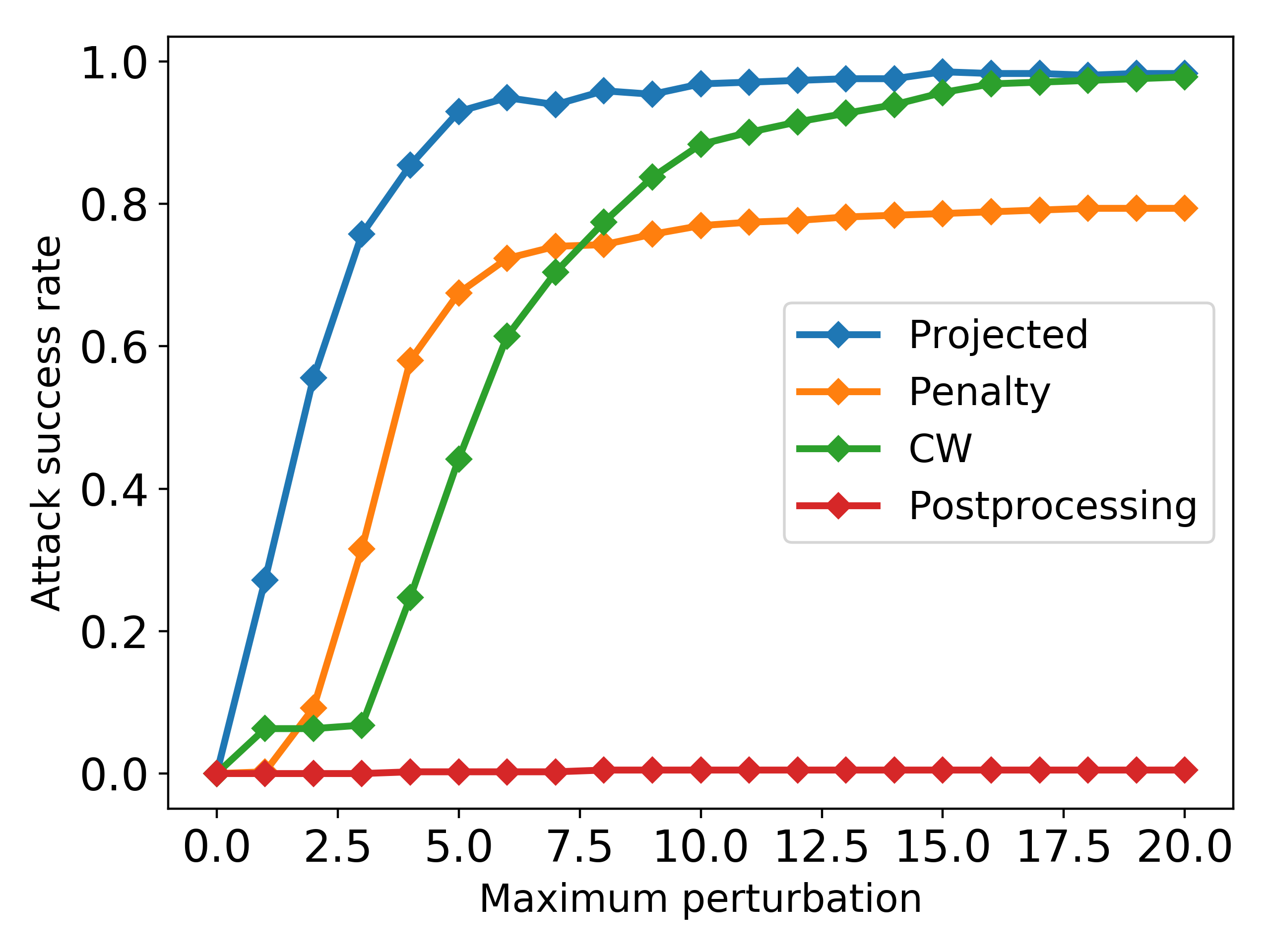
Figure 8. Malicious domain classifier attacks. FENCE Projected attacks perform best. C&W does not generate feasible adversarial examples.

Number and importance of features modified. We compare how many features were modified in order to generate each of the three attacks: Projected, Penalty, and C&W.

It is not surprising that the C&W attack modifies almost all features, as it works in $L_{2}$ norms without any restriction in feature space. Both the Projected and the Penalty attacks modify a much smaller number of features (4 on average).

We are interested in determining if there is a relationship between feature importance and choice of feature by the optimization algorithm. For additional details on feature description, we include the list of features that can be modified in Table 6.

We observe that features of higher importance are chosen more frequently by the optimization attack. However, since we are modifying the representative feature in each family, the number of modifications on the representative feature is usually higher (it accumulates all the importance of the features in that family). For the Bytes family, feature 3 (number of received bytes) is the representative feature and it is updated more than 350 times. However, for features that have no dependencies (e.g., 68 – number of levels in the domain, 69 – number of sub-domains, 71 – domain registration age, and 72 – domain registration validity), the number of updates corresponds to the feature importance.

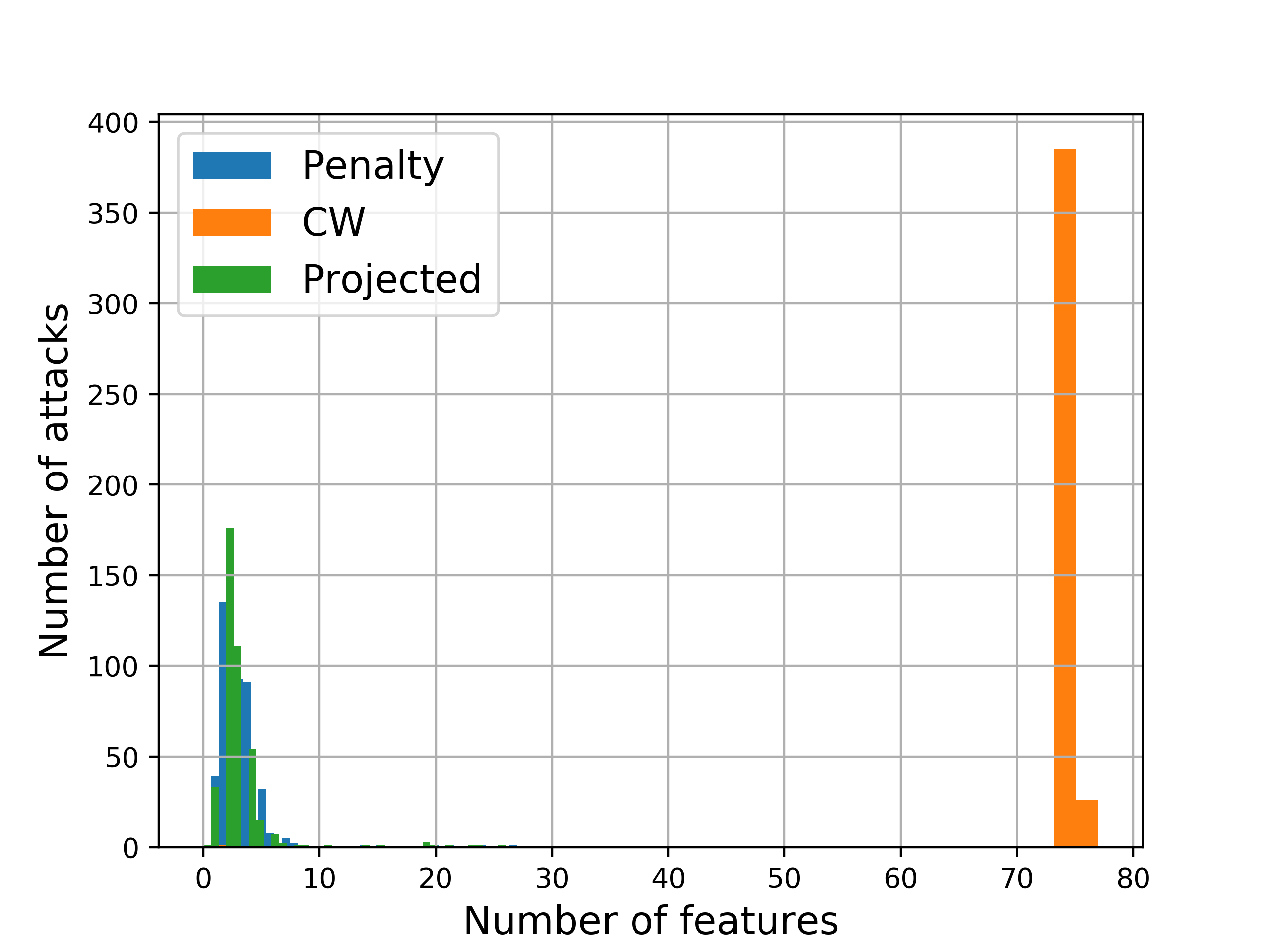
(a) Histogram on feature
modifications.

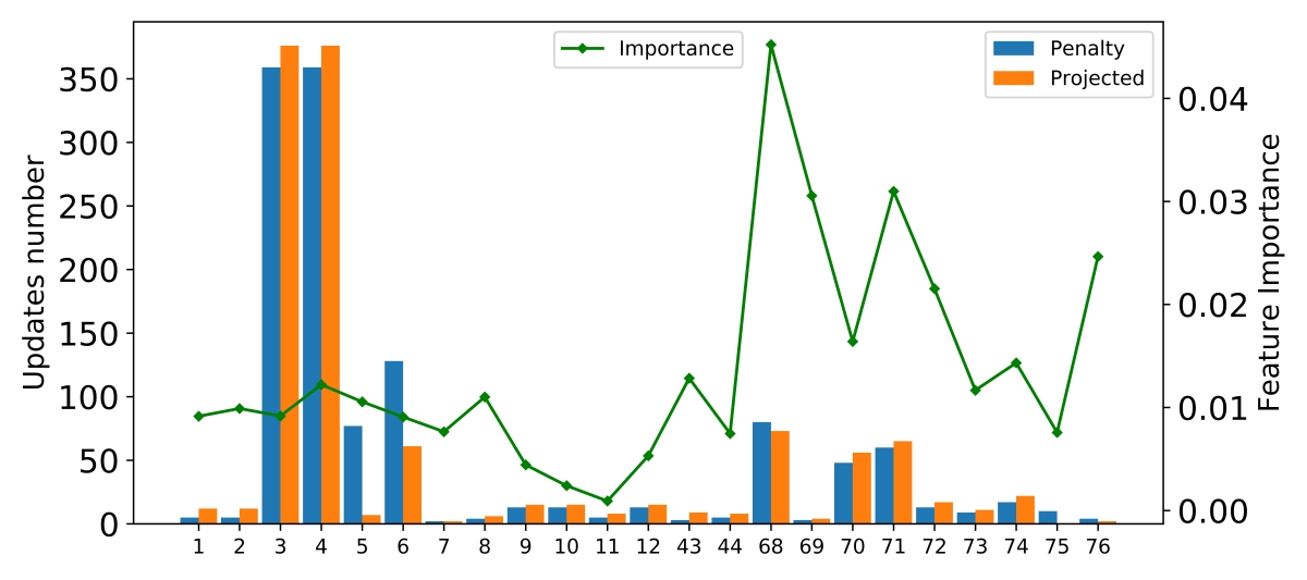
(b) Number of updates (left),
feature importance (right).

Figure 9. Feature modification statistics for malicious domain classifier.

6.3. Misclassification of $\mathsf{Benign}$ Samples as $\mathsf{Malicious}$

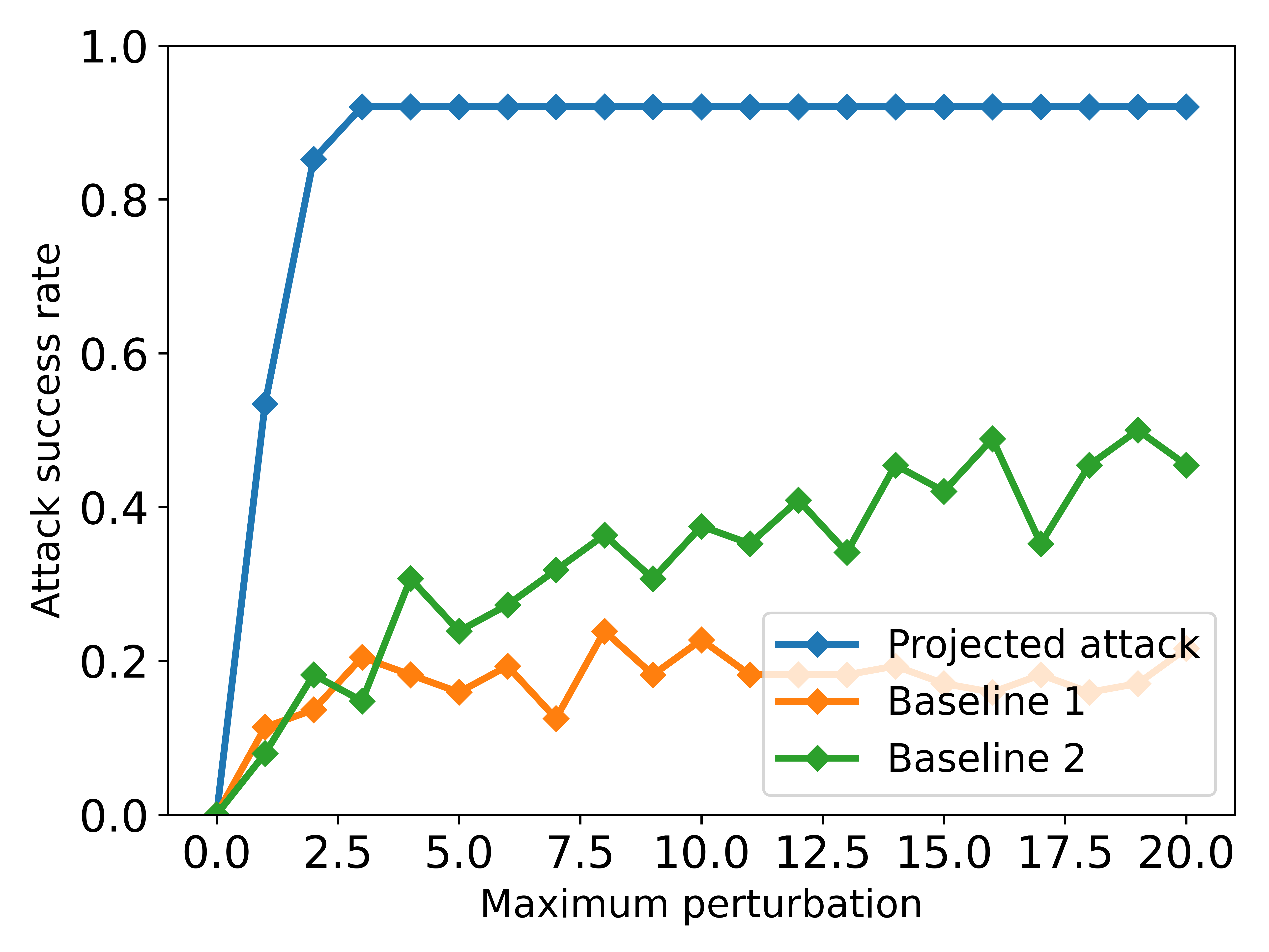
(a) Projected attack.

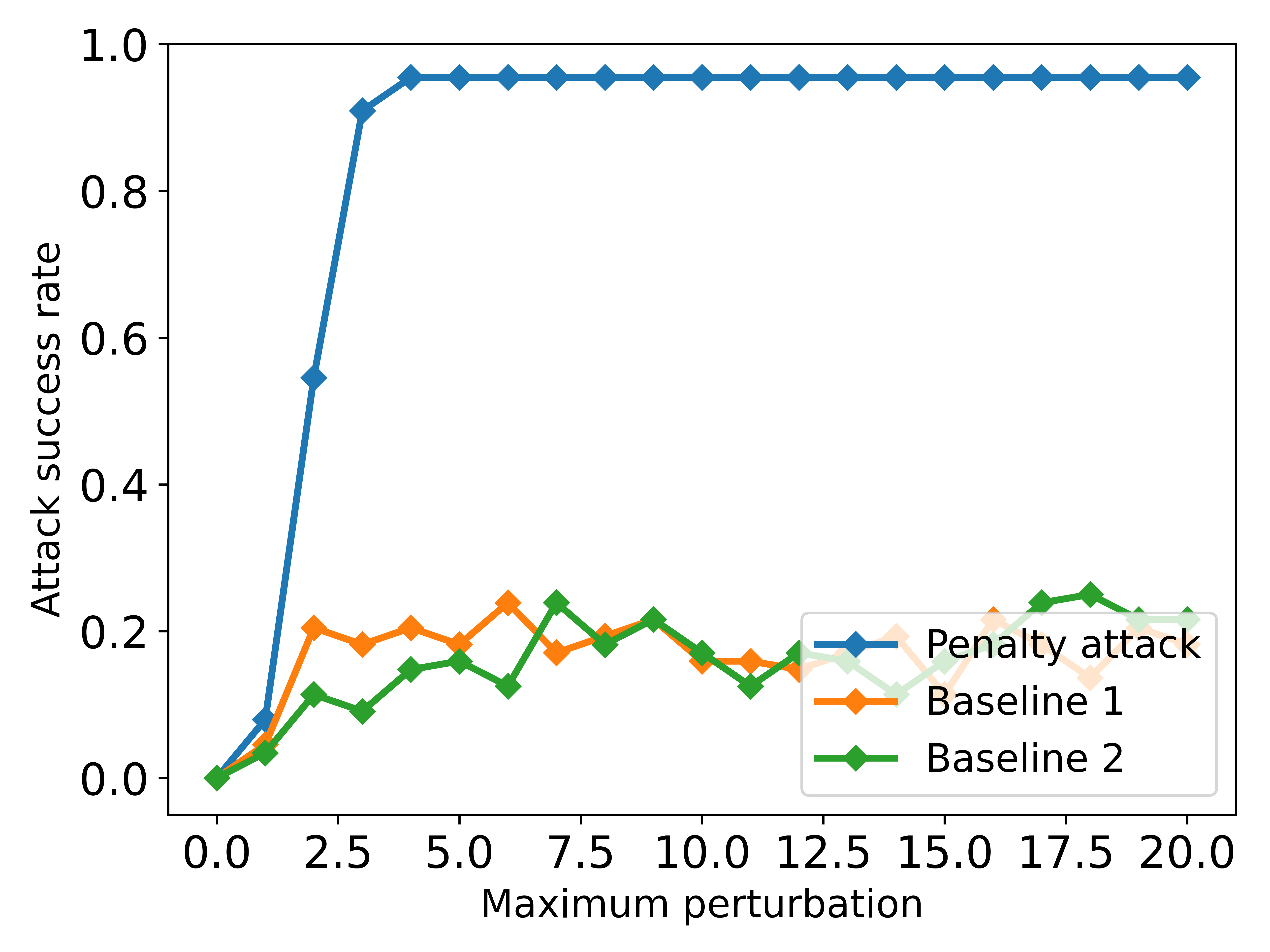
(b) Penalty attack.

Figure 10. FENCE attack results for misclassification of $\mathsf{Benign}$ samples to $\mathsf{Malicious}$.

We ran the Projected and Penalty attacks for changing the classification of $\mathsf{Benign}$ inputs to $\mathsf{Malicious}$ to show the generality of the FENCE framework. The success rate of the attacks compared to two baseline attacks for balanced classes is illustrated in Figure 10. Both attacks achieve high success rate: At $L_{2}=20$ the Projected attack reaches 92% success rate and the Penalty attack reaches 95% success rate. The FENCE attack performs significantly better compared to both baseline attacks.

6.4. Attack Transferability

We consider here a threat model in which the adversary only knows the feature representation, but not the exact ML model or the training data. One approach to generate adversarial examples is through transferability (Papernot et al., 2016a; Liu et al., 2016; Tramèr et al., 2017; Suciu et al., 2018b; Demontis et al., 2019). We perform several experiments to test the transferability of the Projected attacks against FFNN to logistic regression (LR) and random forest (RF). Models were trained with different data and we vary the imbalance ratio. The results are in Table 16. We observe that the largest transferability rate to both LR and RF is for the highest imbalanced ratio of 50 (98.2% adversarial examples transfer to LR and 94.8% to RF). As we increase the imbalance ratio, the transfer rate increases and the transferability rate to LR is lower than to RF.

Ratio	FFNN	LR	RF
1	100%	40%	51.7%
5	93.3%	66.5%	82.9%
15	99%	60.9%	90.2%
25	100%	47.6%	68.8%
50	100%	98.2%	94.8%

Table 16. Transferability of adversarial examples from FFNN to LR and RF. We vary the imbalance ratio in training. Column FFNN shows the white-box attack success rate.

We also look at the transferability between different FFNN architectures trained on different datasets (results in Table 17). The attacks transfer best at the highest imbalance ratio (with a success rate higher than 96%), confirming that weaker models are easier to attack.

Ratio	DNN1	DNN2	DNN3
	[80, 50]	[160, 80]	[100, 50, 25]
1	100%	57.6%	42.3%
5	93.3%	73.6%	58.6%
15	99%	78.6%	52.4%
25	100%	51.4%	45.3%
50	100%	96%	97.1%

Table 17. Transferability between architectures (number of neurons per layer in the second row). Adversarial examples computed for DNN1 are transferred to DNN2 and DNN3.

6.5. Mitigations

Finally, we looked at defensive approaches to increase the FFNN robustness against the FENCE evasion attack. A well-known defensive technique is adversarial training (Goodfellow et al., 2014; Madry et al., 2017). We trained FFNN using adversarial training with the Projected attack at $L_{2}$ distance 20. We trained the model adversarially for 11 epochs and obtained the AUC score of 89% (each epoch takes approximately 7 hours). We measured the Projected attack’s success rate for the balanced case against the standard and adversarially training models in Figure 11. Interestingly, the success rate of the evasion attacks significantly drops for the adversarially-trained model and reaches only 16.5% at 20 $L_{2}$ distance. This demonstrates that adversarial training is a promising direction for designing robust ML models for security. We plan to investigate it further and optimize its design in future work.

Figure 11. Success rate of the FENCE Projected attack against adversarially and standard trained model.

7. Related Work

Adversarial machine learning studies ML vulnerabilities against attacks (Huang et al., 2011). Research on the robustness of DNNs at testing time started with the work of Biggio et al. (Biggio et al., 2013) and Szegedy et al. (Szegedy et al., 2014). They showed that classifiers are vulnerable to adversarial examples generated with minimal perturbation to testing inputs. Since then, the area of adversarial ML has received a lot of attention, with the majority of work focused on evasion attacks (at testing time), e.g., (Goodfellow et al., 2014; Kurakin et al., 2016; Papernot et al., 2017b, a; Carlini and Wagner, 2017; Athalye et al., 2018; Sharif et al., 2019). Other classes of attacks include poisoning (e.g., (Biggio et al., 2012; Xiao et al., 2015)) and privacy attacks (e.g., (Fredrikson et al., 2015; Shokri et al., 2017)), but we focus here on evasion attacks.

Evasion attacks in security. Several evasion attacks have been proposed against models with discrete and constrained input vectors, as encountered in security. The majority of these use datasets with binary features, not considering dependencies in feature space. Biggio et al. (Biggio et al., 2013) use a gradient-based attack to construct adversarial examples for malicious PDF detection by only adding new keywords to PDFs. Grosse et al. (Grosse et al., 2016) leverage the JSMA attack by Papernot et al. (Papernot et al., 2017b) for a malware classification application in which features can be added or removed. Suciu et al. (Suciu et al., 2018a) add bytes to malicious binaries either at the end or in slack regions to create adversarial examples. Kreuk (Kreuk et al., 2018) discover regions in executables that would not affect the intended malware behavior. Kolosnjaji et al. (Kolosnjaji et al., 2018) create gradient-based attack against malware detection DNNs that learn from raw bytes, and can create adversarial examples by only changing a few specific bytes at the end of each malware sample. Xu et al. (Xu et al., 2016) propose a black-box attack based on genetic algorithms for manipulating PDF files while maintaining the required format. Dang et al. (Dang et al., 2017) propose a black-box attack against PDF malware classifiers that uses hill-climbing over a set of feasible transformations. Anderson et al. (Anderson et al., 2018) construct a general black-box framework based on reinforcement learning for attacking static portable executable anti-malware engines. Kulynych et al. (Kulynych et al., 2018) propose a graphical framework for discrete domains with guarantees of minimal adversarial cost. Recently, Pierazzi et al. (Pierazzi et al., 2019) define a formalization for the domain-space attacks, along with a new white-box attack against Android malware classification. The authors use automated software transplantation to extract slices of bytecode from benign applications and inject them into a malicious host to mimic the benign activity and evade the classifier. Chen et al.  (Chen et al., 2017) proposed an evasion attack called EvnAttack on malware present in portable Windows executable files, where input vectors are binary features each representing an API call to Windows.

Evasion attacks for network traffic classifiers include: Apruzesse et al. (Apruzzese and Colajanni, 2018) analyzing the robustness of random forest for botnet classification; Clements et al. (Clements et al., 2019) evaluating the robustness of an anomaly detection method (Mirsky et al., 2018) against existing attacks; and De Lucia et al. (De Lucia and Cotton, 2019) attacking an SVM for network scanning detection. A number of papers perform attacks against intrusion detection systems (IDS). Among them, Warzynski and Kołaczek  (Warzyński and Kołaczek, 2018) consider an FGSM attack under L1 norm against IDS and illustrates the ability of the generated adversarial example to evade the classifier. Rigaki et al.  (Rigaki, 2017) generate targeted attacks by using FGSM and JSMA to evade decision tree, random forest, linear SVM, voting ensembles of the previous three classifiers, and a multi-layer perceptron (MLP) neural network IDS. Similarly, Wang et al  (Wang, 2018) leveraged FGSM, JSMA, Deepfool, and Carlini-Wagner to attack an MLP neural network for intrusion detection. Yang et al.  (Yang et al., 2018b) used Carlini-Wagner, a GAN attack, and black-box ZOO attacks against IDS DNNs. In their work Martins et al. (Martins et al., 2019) tested the performance of FGSM, JSMA, Deepfool, and Carlini-Wagner attacks against decision tree, random forest, SVM, naive Bayes, neural networks, and denoising autoencoders intrusion detection models. Wu et al.  (Wu et al., 2019) applied deep reinforcement learning to generate adversarial attacks on botnet attacks. Yan et al.  (Yan et al., 2019) generate adversarial examples for denial of service attacks. Lin et al.  (Lin et al., 2018) use a modification of GAN called IDSGAN to produce adversarial examples while retaining functional features of the attack.

Evasion attacks with dependency constraints. A number of attacks that preserve constraints between extracted features in security exist in the literature. We survey these papers in greater detail and add a comparison to FENCE in Table 18.

Alhajjar et al. (Alhajjar et al., 2020) explore the use of evolutionary computations and generative adversarial networks as a tool for crafting adversarial examples that aim to evade machine learning models used for network traffic classification. These strategies were applied to the NSL-KDD and UNSW-NB15 datasets. The paper operates only in features space, and the following dependencies are preserved: binary features, linear dependencies and features that can only be increased. There is no limitation on the amount of perturbations, as the authors claim that large changes in data are not subject to easy recognition by human observers. The percent of successful evasion for multi-layer perceptron (MLP) is much worse for both datasets than in FENCE: maximum 86.18% for NSL-KDD using GANs, and 55.10% for the UNSW-NB15 dataset. In contrast, FENCE minimizes the perturbation needed for evasion, preserves a much larger number of dependencies, such as non-linear, statistical, or combination of them, achieving a higher success rate.

Granados et al. (Granados et al., 2020) introduce Restricted Traffic Distribution Attack (RTDA) against network traffic classifiers, which is based on the Carlini and Wagner attack. In order to ensure the feasibility of adversarial examples, the attack only modifies the features corresponding to different percentiles for packet sizes by increasing their values and preserving the monotonic non-decreasing property of generated packet-size distribution. The attacker operates only in feature space, and there is no limit on bytes added to the packet, which may result in the packet sizes that are larger than allowed by network protocols. In contrast, FENCE  generates more realistic attacks in the real-world scenario, by adding new connections of different types (UDP/TCP) and on different ports. Moreover, FENCE ensures feasibility by preserving packet sizes, connection durations, and other network traffic characteristics according to the constraints of network protocols.

Abusnaina et al. (Abusnaina et al., 2019) present MergeFlow attack against DDoS detection models. They create adversarial examples by combining features from existing network flow with a representative mask flow from the target class. The features are combined either through averaging for ratio features or accumulating for count-based features. This attack preserves dependencies between features but generates large perturbations. Abusnaina et al. present similar ideas against graph-based IoT Malware Detection System that creates realistic adversarial examples by combining the original graph with a selected targeted class.

Sadeghzadeh et al. (Sadeghzadeh et al., 2021) introduce an adversarial network traffic attack (ANT) that uses a universal adversarial perturbation (UAP) generating method. To generate ANT they introduce the following three types of attack: AdvPad injects UAP to the content of packets to evaluate the robustness of packet classifiers, AdvPay injects UAP into payload if a dummy packet to evaluate flow-based classifiers, and AdvBurst modifies a burst of the flow to test the robustness of flow time-series classifiers. In order to generate the UAP, a set of flows or packets from a particular class is leveraged and the UAP is inserted into new incoming traffic of that class. This attack works in the domain space by inserting payload, dummy packet with payload, or the sequence of packets with statistical features. All perturbations are calculated by inserting the randomly initialized perturbation vector into examples from the target class and optimizing the loss function towards the selected class for some number of iterations. Sequences of bytes were used for training the classifiers, thus, there are no dependencies in the domain space. The only thing that needs to be preserved is the range for the number of bytes achieved by performing the clipping operation while computing UAP.

Han et al. (Han et al., 2020) propose a practical traffic-space evasion attack against Network Intrusion Detection System (NIDS). The attacker can modify the original traffic generated from devices he controls at an affordable overhead. It has two main steps: finding the adversarial feature vector which can be classified as benign but is close to the malicious feature vector in terms of features’ values (lies in the low-confidence region of the classifier) using the GAN model and transforming malicious original traffic to transfer its features to the closest adversarial ones preserving its functionality using particle swarm optimization (PSO). While performing the second step authors allow only to modify the interarrival time of packets in the original traffic, and for the injected crafted traffic the attacker is able to alter the interarrival time of packets, protocol layer of packets, and payload size. The budget overhead for the number of buckets and time elapsed is controlled by the rate of the original traffic. Feature dependencies are preserved in the domain space only, in contrast, FENCE allows to additionally preserve complex mathematical dependencies in feature space.

Chen et al.  (Chen et al., 2020) introduce two types of evasion attacks against machine learning-based intrusion detection systems. The first attack called $Opt$ uses an iterative optimization approach to find the adversarial examples that maximize the probability of malicious output while remaining stealthy and preserving the Range dependency. The second attack detaches the malicious payload from the input vector, and then optimizes the modifiable features based on a GAN under the Range dependency, keeping some features as integers. Thus, both attacks preserve only domain-specific dependencies, while FENCE is capable of satisfying a larger amount of domain dependencies as well as a list of mathematical constraints.

None of these previous works can handle the same amount of domain and mathematical dependencies supported by our FENCE framework. In Table 18 we compare FENCE with these attacks against network traffic classifiers and include the list of supported constraints.

Paper	Classifiers	Algorithm	Domain	Mathematical
			Dependencies	Dependencies
FENCE	Network Traffic,	Iterative	Ratio	Stat
	Malicious Domains	optimization	Range	Lin
		Projected	OHE	Non-Lin
		Penalty		Combination
Alhajjar et al. (Alhajjar et al., 2020)	Network Traffic	GAN/PSO	OHE	Linear
Granados et al.  (Granados et al., 2020)	Network Traffic	Iterative	Range	Stat
		optimization
Sadeghzadeh et al. (Sadeghzadeh et al., 2021)	Packets	UAP	Range	-
	Network Flows
	Network Bursts
Han et al.  (Han et al., 2020)	Botnet	GAN/PSO	Range	-
Abusnaina et al. (Abusnaina et al., 2019)	DDoS Detection	Sample	Range	-
		injection	Ratio	-
Chen et al. (Chen et al., 2020)	Network Traffic	Iterative	Range	-
		optimization		-
		GAN

Table 18. Comparison to existing work on evasion attacks in cybersecurity domains. We only include methods which respect dependencies in feature space. For each method, we mention the adversarial attack algorithm and the supported feature dependencies.

Evasion attacks in other domains. There is work on designing attacks in other domains, such as audio:  (Gong and Poellabauer, 2017),  (Cisse et al., 2017),  (Zhang et al., 2017),  (Song and Mittal, 2017),  (Schonherr et al., 2018),  (Yakura and Sakuma, 2018),  (Carlini and Wagner, 2018)  (Qin et al., 2019); text:  (Papernot et al., 2016b),  (Ebrahimi et al., 2017),  (Liang et al., 2017),  (Gao et al., 2018),  (Alzantot et al., 2018); and video:  (Li et al., 2019b),  (Hosseini et al., 2017),  (Wei et al., 2018). Physically realizable attacks have been designed for face recognition (Sharif et al., 2016) and vision (Eykholt et al., 2018).

Defenses against evasion attacks. Standard methods to defend against adversarial evasion attacks in continuous domains include: adversarial training (Madry et al., 2017), randomized smoothing (Cohen et al., 2019), and defenses based on the detection of adversarial examples (Roth et al., 2019; Li et al., 2019a; Yin et al., 2019; Yu et al., 2019; Yang et al., 2018a). Randomized smoothing provides certifiable guarantees, but unfortunately, it cannot be directly applied in discrete domains because it requires the classifier to be evaluated on inputs perturbed with Gaussian noise. Therefore, we are not aware of any uses of randomized smoothing and similar randomization-based mechanism for cyber security defenses.

Defenses based on adversarial training have been used in cyber security. For instance, Abusnaina et al. (Abusnaina et al., 2019) validate whether adversarial training improves the robustness of the DDoS detection system. They show that adversarial training is able to improve the robustness of the anomaly classification model, but only for certain types of adversarial examples included in the adversarial training. Hashem et al. (Hashemi and Keller, 2020) develop a network intrusion detection system that utilizes a novel reconstruction from partial observation method to build a more accurate anomaly detection model. The method also improves robustness to adversarial examples.

Methods for the detection of adversarial examples in security have been proposed. For example, Wang et al.  (Wang et al., 2021) propose a defense mechanism against adversarial examples for NIDS, which exploits the inconsistency between manifold evaluation and model inference along with the closeness of the resulting adversarial example to the manifold. This allows them to train a logistic regression that predicts whether the input may be considered adversarial or not. In general, a known limitation of detection methods is that they fail in face of adaptive attacks. Tramer et al. (Tramer et al., 2020) showed that multiple detection-based methods (e.g. (Roth et al., 2019)) are not resilient against adaptive attacks, and thus designing detection-based defenses in cyber security which are resilient to adaptive attacks remains an open problem.

8. Conclusions

We showed that evasion attacks against DNNs can be designed to preserve the dependencies in feature space in constrained domains. We proposed a general framework FENCE for generating adversarial examples that respects mathematical dependencies and domain-specific constraints imposed by these applications. We demonstrated evasion attacks that insert a small number of network connections (12 records in Zeek connection logs) to misclassify $\mathsf{Malicious}$ activity as $\mathsf{Benign}$ in a malicious connection classifier. We also showed that adversarial training has the potential to increase the robustness of classifiers in the malicious domain setting.

Our FENCE framework is not restricted to security applications, and we plan to apply it to healthcare and financial scenarios. An important open problem in this space is how to increase the resilience of DNN classifiers used in critical, constrained applications.

- (1)
- Abusnaina et al. (2019) Ahmed Abusnaina, Aminollah Khormali, DaeHun Nyang, Murat Yuksel, and Aziz Mohaisen. 2019. Examining the robustness of learning-based ddos detection in software defined networks. In 2019 IEEE Conference on Dependable and Secure Computing (DSC). IEEE, 1–8.
- Alhajjar et al. (2020) Elie Alhajjar, Paul Maxwell, and Nathaniel D Bastian. 2020. Adversarial machine learning in network intrusion detection systems. arXiv preprint arXiv:2004.11898 (2020).
- Alzantot et al. (2018) Moustafa Alzantot, Yash Sharma, Ahmed Elgohary, Bo-Jhang Ho, Mani Srivastava, and Kai-Wei Chang. 2018. Generating natural language adversarial examples. arXiv preprint arXiv:1804.07998 (2018).
- Anderson et al. (2018) Hyrum S Anderson, Anant Kharkar, Bobby Filar, David Evans, and Phil Roth. 2018. Learning to evade static PE machine learning malware models via reinforcement learning. arXiv preprint arXiv:1801.08917 (2018).
- Apruzzese and Colajanni (2018) Giovanni Apruzzese and Michele Colajanni. 2018. Evading Botnet Detectors Based on Flows and Random Forest with Adversarial Samples. 1–8. https://doi.org/10.1109/NCA.2018.8548327
- Athalye et al. (2018) Anish Athalye, Nicholas Carlini, and David Wagner. 2018. Obfuscated gradients give a false sense of security: Circumventing defenses to adversarial examples. arXiv preprint arXiv:1802.00420 (2018).
- Bartos et al. (2016) Karel Bartos, Michal Sofka, and Vojtech Franc. 2016. Optimized Invariant Representation of Network Traffic for Detecting Unseen Malware Variants. In 25th USENIX Security Symposium (USENIX Security 16). USENIX Association, 807–822.
- Biggio et al. (2013) Battista Biggio, Igino Corona, Davide Maiorca, Blaine Nelson, Nedim Srndic, Pavel Laskov, Giorgio Giacinto, and Fabio Roli. 2013. Evasion Attacks against Machine Learning at Test Time. In Proc. Joint European Conference on Machine Learning and Knowledge Discovery in Databases (ECML PKDD).
- Biggio et al. (2012) Battista Biggio, Blaine Nelson, and Pavel Laskov. 2012. Poisoning attacks against support vector machines. In ICML.
- Bilge et al. (2011) Leyla Bilge, Engin Kirda, Kruegel Christopher, and Marco Balduzzi. 2011. EXPOSURE: Finding Malicious Domains Using Passive DNS Analysis. In Proc. 18th Symposium on Network and Distributed System Security (NDSS).
- Carlini and Wagner (2017) Nicholas Carlini and David Wagner. 2017. Towards Evaluating the Robustness of Neural Networks. In Proc. IEEE Security and Privacy Symposium.
- Carlini and Wagner (2018) Nicholas Carlini and David A. Wagner. 2018. Audio Adversarial Examples: Targeted Attacks on Speech-to-Text. CoRR abs/1801.01944 (2018). arXiv:1801.01944 http://arxiv.org/abs/1801.01944
- Chen et al. (2020) Jiming Chen, Xiangshan Gao, Ruilong Deng, Yang He, Chongrong Fang, and Peng Cheng. 2020. Generating Adversarial Examples against Machine Learning based Intrusion Detector in Industrial Control Systems. IEEE Transactions on Dependable and Secure Computing (2020).
- Chen et al. (2017) Lingwei Chen, Yanfang Ye, and Thirimachos Bourlai. 2017. Adversarial machine learning in malware detection: Arms race between evasion attack and defense. In 2017 European Intelligence and Security Informatics Conference (EISIC). IEEE, 99–106.
- Cisse et al. (2017) Moustapha Cisse, Yossi Adi, Natalia Neverova, and Joseph Keshet. 2017. Houdini: Fooling deep structured prediction models. arXiv preprint arXiv:1707.05373 (2017).
- Clements et al. (2019) Joseph Clements, Yuzhe Yang, Ankur Sharma, Hongxin Hu, and Yingjie Lao. 2019. Rallying Adversarial Techniques against Deep Learning for Network Security. arXiv preprint arXiv:1903.11688 (2019).
- Cohen et al. (2019) Jeremy Cohen, Elan Rosenfeld, and Zico Kolter. 2019. Certified adversarial robustness via randomized smoothing. In International Conference on Machine Learning. PMLR, 1310–1320.
- Dang et al. (2017) Hung Dang, Yue Huang, and Ee-Chien Chang. 2017. Evading classifiers by morphing in the dark. In Proceedings of the 2017 ACM SIGSAC Conference on Computer and Communications Security. ACM, 119–133.
- De Lucia and Cotton (2019) Michael J De Lucia and Chase Cotton. 2019. Adversarial Machine Learning for Cyber Security. Journal Of Information Systems Applied Research (2019).
- Demontis et al. (2019) Ambra Demontis, Marco Melis, Maura Pintor, Matthew Jagielski, Battista Biggio, Alina Oprea, Cristina Nita-Rotaru, and Fabio Roli. 2019. Why do adversarial attacks transfer? Explaining transferability of evasion and poisoning attacks. In 28th USENIX Security Symposium (USENIX Security 19). 321–338.
- Ebrahimi et al. (2017) Javid Ebrahimi, Anyi Rao, Daniel Lowd, and Dejing Dou. 2017. Hotflip: White-box adversarial examples for text classification. arXiv preprint arXiv:1712.06751 (2017).
- Eykholt et al. (2018) Kevin Eykholt, Ivan Evtimov, Earlence Fernandes, Bo Li, Amir Rahmati, Chaowei Xiao, Atul Prakash, Tadayoshi Kohno, and Dawn Xiaodong Song. 2018. Robust Physical-World Attacks on Deep Learning Visual Classification. 2018 IEEE/CVF Conference on Computer Vision and Pattern Recognition (2018), 1625–1634.
- Fredrikson et al. (2015) Matt Fredrikson, Somesh Jha, and Thomas Ristenpart. 2015. Model Inversion Attacks that Exploit Confidence Information and Basic Countermeasures. In Proceedings of the 22nd ACM Conference on Computer and Communications Security (CCS).
- Gao et al. (2018) Ji Gao, Jack Lanchantin, Mary Lou Soffa, and Yanjun Qi. 2018. Black-box generation of adversarial text sequences to evade deep learning classifiers. In 2018 IEEE Security and Privacy Workshops (SPW). IEEE, 50–56.
- Garcia et al. (2014) Sebastian Garcia, Martin Grill, Jan Stiborek, and Alejandro Zunino. 2014. An empirical comparison of botnet detection methods. Computers and Security 45 (2014), 100–123.
- Gong and Poellabauer (2017) Yuan Gong and Christian Poellabauer. 2017. Crafting adversarial examples for speech paralinguistics applications. arXiv preprint arXiv:1711.03280 (2017).
- Goodfellow et al. (2014) Ian J. Goodfellow, Jonathon Shlens, and Christian Szegedy. 2014. Explaining and Harnessing Adversarial Examples. arXiv:1412.6572.
- Granados et al. (2020) Alonso Granados, Mohammad Sujan Miah, Anthony Ortiz, and Christopher Kiekintveld. 2020. A Realistic Approach for Network Traffic Obfuscation Using Adversarial Machine Learning. In International Conference on Decision and Game Theory for Security. Springer, 45–57.
- Grosse et al. (2017) Kathrin Grosse, Praveen Manoharan, Nicolas Papernot, Michael Backes, and Patrick McDaniel. 2017. On the (Statistical) Detection of Adversarial Examples. arXiv:1702.06280.
- Grosse et al. (2016) Kathrin Grosse, Nicolas Papernot, Praveen Manoharan, Michael Backes, and Patrick McDaniel. 2016. Adversarial perturbations against deep neural networks for malware classification. arXiv preprint arXiv:1606.04435 (2016).
- Han et al. (2020) Dongqi Han, Zhiliang Wang, Ying Zhong, Wenqi Chen, Jiahai Yang, Shuqiang Lu, Xingang Shi, and Xia Yin. 2020. Practical traffic-space adversarial attacks on learning-based nidss. arXiv preprint arXiv:2005.07519 (2020).
- Hashemi and Keller (2020) Mohammad J Hashemi and Eric Keller. 2020. Enhancing robustness against adversarial examples in network intrusion detection systems. In 2020 IEEE Conference on Network Function Virtualization and Software Defined Networks (NFV-SDN). IEEE, 37–43.
- Hosseini et al. (2017) Hossein Hosseini, Baicen Xiao, Andrew Clark, and Radha Poovendran. 2017. Attacking automatic video analysis algorithms: A case study of google cloud video intelligence api. In Proceedings of the 2017 on Multimedia Privacy and Security. ACM, 21–32.
- Hu et al. (2016) Xin Hu, Jiyong Jang, Marc Ph. Stoecklin, Ting Wang, Douglas Lee Schales, Dhilung Kirat, and Josyula R. Rao. 2016. BAYWATCH: Robust Beaconing Detection to Identify Infected Hosts in Large-Scale Enterprise Networks. In DSN. IEEE Computer Society, 479–490.
- Huang et al. (2011) Ling Huang, Anthony D Joseph, Blaine Nelson, Benjamin IP Rubinstein, and JD Tygar. 2011. Adversarial machine learning. In Proceedings of the 4th ACM workshop on Security and artificial intelligence. ACM, 43–58.
- Kolosnjaji et al. (2018) Bojan Kolosnjaji, Ambra Demontis, Battista Biggio, Davide Maiorca, Giorgio Giacinto, Claudia Eckert, and Fabio Roli. 2018. Adversarial malware binaries: Evading deep learning for malware detection in executables. In 2018 26th European Signal Processing Conference (EUSIPCO). IEEE, 533–537.
- Kreuk et al. (2018) Felix Kreuk, Assi Barak, Shir Aviv-Reuven, Moran Baruch, Benny Pinkas, and Joseph Keshet. 2018. Deceiving end-to-end deep learning malware detectors using adversarial examples. arXiv preprint arXiv:1802.04528 (2018).
- Kulynych et al. (2018) Bogdan Kulynych, Jamie Hayes, Nikita Samarin, and Carmela Troncoso. 2018. Evading classifiers in discrete domains with provable optimality guarantees. arXiv preprint arXiv:1810.10939 (2018).
- Kurakin et al. (2016) Alexey Kurakin, Ian Goodfellow, and Samy Bengio. 2016. Adversarial examples in the physical world. arXiv preprint arXiv:1607.02533 (2016).
- Li et al. (2019b) Shasha Li, Ajaya Neupane, Sujoy Paul, Chengyu Song, Srikanth V Krishnamurthy, Amit K Roy-Chowdhury, and Ananthram Swami. 2019b. Stealthy Adversarial Perturbations Against Real-Time Video Classification Systems.. In NDSS.
- Li et al. (2019a) Yingzhen Li, John Bradshaw, and Yash Sharma. 2019a. Are generative classifiers more robust to adversarial attacks?. In International Conference on Machine Learning. PMLR, 3804–3814.
- Liang et al. (2017) Bin Liang, Hongcheng Li, Miaoqiang Su, Pan Bian, Xirong Li, and Wenchang Shi. 2017. Deep text classification can be fooled. arXiv preprint arXiv:1704.08006 (2017).
- Lin et al. (2018) Zilong Lin, Yong Shi, and Zhi Xue. 2018. Idsgan: Generative adversarial networks for attack generation against intrusion detection. arXiv preprint arXiv:1809.02077 (2018).
- Liu et al. (2016) Yanpei Liu, Xinyun Chen, Chang Liu, and Dawn Song. 2016. Delving into transferable adversarial examples and black-box attacks. arXiv preprint arXiv:1611.02770 (2016).
- Ma et al. (2009) Justin Ma, Lawrence K. Saul, Stefan Savage, and Geoffrey M. Voelker. 2009. Beyond Blacklists: Learning to Detect Malicious Web Sites from Suspicious URLs. In Proc. 15th ACM International Conference on Knowledge Discovery and Data Mining (KDD).
- Madry et al. (2017) Aleksander Madry, Aleksandar Makelov, Ludwig Schmidt, Dimitris Tsipras, and Adrian Vladu. 2017. Towards deep learning models resistant to adversarial attacks. arXiv preprint arXiv:1706.06083 (2017).
- Martins et al. (2019) Nuno Martins, José Magalhães Cruz, Tiago Cruz, and Pedro Henriques Abreu. 2019. Analyzing the footprint of classifiers in adversarial denial of service contexts. In EPIA Conference on Artificial Intelligence. Springer, 256–267.
- Mirsky et al. (2018) Yisroel Mirsky, Tomer Doitshman, Yuval Elovici, and Asaf Shabtai. 2018. Kitsune: an ensemble of autoencoders for online network intrusion detection. arXiv preprint arXiv:1802.09089 (2018).
- Ongun et al. (2019) Talha Ongun, Timothy Sakharaov, Simona Boboila, Alina Oprea, and Tina Eliassi-Rad. 2019. On Designing Machine Learning Models for Malicious Network Traffic Classification. arXiv preprint arXiv:1907.04846 (2019).
- Oprea et al. (2018) Alina Oprea, Zhou Li, Robin Norris, and Kevin Bowers. 2018. MADE: Security Analytics for Enterprise Threat Detection. In Proceedings of the 34th Annual Computer Security Applications Conference. ACM, 124–136.
- Papernot et al. (2016a) Nicolas Papernot, Patrick McDaniel, and Ian Goodfellow. 2016a. Transferability in machine learning: from phenomena to black-box attacks using adversarial samples. arXiv preprint arXiv:1605.07277 (2016).
- Papernot et al. (2017a) Nicolas Papernot, Patrick McDaniel, Ian Goodfellow, Somesh Jha, Z Berkay Celik, and Ananthram Swami. 2017a. Practical Black-Box Attacks against Machine Learning. In Proceedings of the ACM SIGSAC Asia Conference on Computer and Communications Security (AsiaCCS).
- Papernot et al. (2017b) Nicolas Papernot, Patrick McDaniel, Somesh Jha, Matt Fredrikson, Z. Berkay Celik, and Ananthram Swami. 2017b. The Limitations of Deep Learning in Adversarial Settings. In Proc. IEEE European Security and Privacy Symposium (Euro S&P).
- Papernot et al. (2016b) Nicolas Papernot, Patrick McDaniel, Ananthram Swami, and Richard Harang. 2016b. Crafting adversarial input sequences for recurrent neural networks. In MILCOM 2016-2016 IEEE Military Communications Conference. IEEE, 49–54.
- Pierazzi et al. (2019) Fabio Pierazzi, Feargus Pendlebury, Jacopo Cortellazzi, and Lorenzo Cavallaro. 2019. Intriguing Properties of Adversarial ML Attacks in the Problem Space. arXiv preprint arXiv:1911.02142 (2019).
- Qin et al. (2019) Yao Qin, Nicholas Carlini, Ian Goodfellow, Garrison Cottrell, and Colin Raffel. 2019. Imperceptible, robust, and targeted adversarial examples for automatic speech recognition. arXiv preprint arXiv:1903.10346 (2019).
- Rigaki (2017) Maria Rigaki. 2017. Adversarial deep learning against intrusion detection classifiers.
- Roth et al. (2019) Kevin Roth, Yannic Kilcher, and Thomas Hofmann. 2019. The odds are odd: A statistical test for detecting adversarial examples. arXiv preprint arXiv:1902.04818 (2019).
- Sadeghzadeh et al. (2021) Amir Mahdi Sadeghzadeh, Saeed Shiravi, and Rasool Jalili. 2021. Adversarial Network Traffic: Towards Evaluating the Robustness of Deep-Learning-Based Network Traffic Classification. IEEE Transactions on Network and Service Management 18, 2 (2021), 1962–1976.
- Schonherr et al. (2018) Lea Schonherr, Katharina Kohls, Steffen Zeiler, Thorsten Holz, and Dorothea Kolossa. 2018. Adversarial attacks against automatic speech recognition systems via psychoacoustic hiding. arXiv preprint arXiv:1808.05665 (2018).
- Sharif et al. (2016) Mahmood Sharif, Sruti Bhagavatula, Lujo Bauer, and Michael K. Reiter. 2016. Accessorize to a Crime: Real and Stealthy Attacks on State-of-the-Art Face Recognition. In Proceedings of the 2016 ACM SIGSAC Conference on Computer and Communications Security (Vienna, Austria) (CCS ’16). ACM, New York, NY, USA, 1528–1540. https://doi.org/10.1145/2976749.2978392
- Sharif et al. (2019) Mahmood Sharif, Sruti Bhagavatula, Lujo Bauer, and Michael K Reiter. 2019. A general framework for adversarial examples with objectives. ACM Transactions on Privacy and Security (TOPS) 22, 3 (2019), 1–30.
- Shokri et al. (2017) Reza Shokri, Marco Stronati, Congzheng Song, and Vitaly Shmatikov. 2017. Membership Inference Attacks against Machine Learning Models. In Proc. IEEE Security and Privacy Symposium (S&P).
- Song and Mittal (2017) Liwei Song and Prateek Mittal. 2017. Inaudible voice commands. arXiv preprint arXiv:1708.07238 (2017).
- Srndic and Laskov (2014) Nedim Srndic and Pavel Laskov. 2014. Practical Evasion of a Learning-Based Classifier: A Case Study. In Proc. IEEE Security and Privacy Symposium.
- Suciu et al. (2018a) Octavian Suciu, Scott E Coull, and Jeffrey Johns. 2018a. Exploring adversarial examples in malware detection. arXiv preprint arXiv:1810.08280 (2018).
- Suciu et al. (2018b) Octavian Suciu, Radu Marginean, Yigitcan Kaya, Hal Daume III, and Tudor Dumitras. 2018b. When does machine learning {}? generalized transferability for evasion and poisoning attacks. In 27th USENIX Security Symposium (USENIX Security 18). 1299–1316.
- Szegedy et al. (2014) Christian Szegedy, Wojciech Zaremba, Ilya Sutskever, Joan Bruna, Dumitru Erhan, Ian Goodfellow, and Rob Fergus. 2014. Intriguing properties of neural networks. arXiv:1312.6199.
- Tong et al. (2019) Liang Tong, Bo Li, Chen Hajaj, Chaowei Xiao, Ning Zhang, and Yevgeniy Vorobeychik. 2019. Improving Robustness of ML Classifiers against Realizable Evasion Attacks Using Conserved Features. In 28th USENIX Security Symposium (USENIX Security 19). USENIX Association, Santa Clara, CA, 285–302. https://www.usenix.org/conference/usenixsecurity19/presentation/tong
- Tramer et al. (2020) Florian Tramer, Nicholas Carlini, Wieland Brendel, and Aleksander Madry. 2020. On adaptive attacks to adversarial example defenses. arXiv preprint arXiv:2002.08347 (2020).
- Tramèr et al. (2017) Florian Tramèr, Nicolas Papernot, Ian Goodfellow, Dan Boneh, and Patrick McDaniel. 2017. The space of transferable adversarial examples. arXiv preprint arXiv:1704.03453 (2017).
- Wang et al. (2021) Ning Wang, Yimin Chen, Yang Hu, Wenjing Lou, and Y Thomas Hou. 2021. MANDA: On Adversarial Example Detection for Network Intrusion Detection System. In IEEE INFOCOM 2021-IEEE Conference on Computer Communications. IEEE, 1–10.
- Wang (2018) Zheng Wang. 2018. Deep learning-based intrusion detection with adversaries. IEEE Access 6 (2018), 38367–38384.
- Warzyński and Kołaczek (2018) Arkadiusz Warzyński and Grzegorz Kołaczek. 2018. Intrusion detection systems vulnerability on adversarial examples. In 2018 Innovations in Intelligent Systems and Applications (INISTA). IEEE, 1–4.
- Wei et al. (2018) Xingxing Wei, Jun Zhu, and Hang Su. 2018. Sparse adversarial perturbations for videos. arXiv preprint arXiv:1803.02536 (2018).
- Wu et al. (2019) Di Wu, Binxing Fang, Junnan Wang, Qixu Liu, and Xiang Cui. 2019. Evading machine learning botnet detection models via deep reinforcement learning. In ICC 2019-2019 IEEE International Conference on Communications (ICC). IEEE, 1–6.
- Xiao et al. (2015) Huang Xiao, Battista Biggio, Gavin Brown, Giorgio Fumera, Claudia Eckert, and Fabio Roli. 2015. Is feature selection secure against training data poisoning?. In Proc. 32nd International Conference on Machine Learning (ICML, Vol. 37). 1689–1698.
- Xu et al. (2016) Weilin Xu, Yanjun Qi, and David Evans. 2016. Automatically evading classifiers. In Proceedings of the 2016 Network and Distributed Systems Symposium. 21–24.
- Yakura and Sakuma (2018) Hiromu Yakura and Jun Sakuma. 2018. Robust audio adversarial example for a physical attack. arXiv preprint arXiv:1810.11793 (2018).
- Yan et al. (2019) Qiao Yan, Mingde Wang, Wenyao Huang, Xupeng Luo, and F Richard Yu. 2019. Automatically synthesizing DoS attack traces using generative adversarial networks. International Journal of Machine Learning and Cybernetics 10, 12 (2019), 3387–3396.
- Yang et al. (2018b) Kaichen Yang, Jianqing Liu, Chi Zhang, and Yuguang Fang. 2018b. Adversarial examples against the deep learning based network intrusion detection systems. In MILCOM 2018-2018 IEEE Military Communications Conference (MILCOM). IEEE, 559–564.
- Yang et al. (2018a) Zhuolin Yang, Bo Li, Pin-Yu Chen, and Dawn Song. 2018a. Characterizing audio adversarial examples using temporal dependency. arXiv preprint arXiv:1809.10875 (2018).
- Yin et al. (2019) Xuwang Yin, Soheil Kolouri, and Gustavo K Rohde. 2019. Adversarial example detection and classification with asymmetrical adversarial training. arXiv preprint arXiv:1905.11475 (2019).
- Yu et al. (2019) Tao Yu, Shengyuan Hu, Chuan Guo, Wei-Lun Chao, and Kilian Q Weinberger. 2019. A new defense against adversarial images: Turning a weakness into a strength. arXiv preprint arXiv:1910.07629 (2019).
- Zhang et al. (2017) Guoming Zhang, Chen Yan, Xiaoyu Ji, Tianchen Zhang, Taimin Zhang, and Wenyuan Xu. 2017. Dolphinattack: Inaudible voice commands. In Proceedings of the 2017 ACM SIGSAC Conference on Computer and Communications Security. ACM, 103–117.