Event-triggered boundary control of constant-parameter reaction–diffusion PDEs: a small-gain approach

Abstract

This paper deals with an event-triggered boundary control of constant-parameters reaction-diffusion PDE systems. The approach relies on the emulation of backstepping control along with a suitable triggering condition which establishes the time instants at which the control value needs to be sampled/updated. In this paper, it is shown that under the proposed event-triggered boundary control, there exists a minimal dwell-time (independent of the initial condition) between two triggering times and furthermore the well-posedness and global exponential stability are guaranteed. The analysis follows small-gain arguments and builds on recent papers on sampled-data control for this kind of PDE. A simulation example is presented to validate the theoretical results.

,  ,

1 Introduction

Control and estimation strategies must be implemented and validated into digital platforms. It is important to study carefully the issues concerning digital control such as sampling. This is because, if sampling is not addressed properly, the stability and estimation properties may be lost. For finite-dimensional systems, namely networked control systems modeled by ordinary differential equations (ODEs), digital control has been extensively developed and several schemes for discretization and for sampling in time continuous-time controllers have been investigated, e.g., by sampled-data control [11] and event-triggered control strategies [29, 10, 24, 21, 9, 25, 13, 22]. The latter has become popular and promising due to not only its efficient way of using communication and computational resources by updating the control value aperiodically (only when needed) but also due to its rigorous way of implementing continuous-time controllers into digital platforms.

In general, event-triggered control includes two main components: a feedback control law which stabilizes the system and an event-triggered mechanism which contains a triggering condition that determines the time instants at which the control needs to be updated. Two general approaches exist for the design: Emulation from which the controller is a priori predesigned and only the event-triggered algorithm has to be designed (as in e.g. [29]) and Co-design, where the joint design of the control law and the event-triggering mechanism is performed simultaneously (see e.g. [27]).

Nevertheless, for partial differential equations (PDEs) sampled-data and event-triggered control strategies without model reduction have not achieved a sufficient level of maturity as in the finite-dimensional case. It has not been sufficiently clear (from theoretical and practical point of view) how fast sampling the in-domain or the boundary continuous-time controllers should be for preserving both stability and convergence properties of PDE systems. Few approaches on sampled-data and event-triggered control of parabolic PDEs are considered in [8, 15, 26], [32, 12]. In the context of abstract formulation of distributed parameter systems, sampled-data control is investigated in [23] and [30]. For hyperbolic PDEs, sampled-data control is studied in [4] and [14]. Some recent works have introduced event-triggered control strategies for linear hyperbolic PDEs under an emulation approach [5, 6, 7]. In [5] and [6], for instance, event-triggered boundary controllers for linear conservation laws using output feedback are studied by following Lyapunov techniques (inspired by [1]). In [7], the approach relies on the backstepping method for coupled system of balance laws (inspired by [31, 19]) which leads to a full-state feedback control which is sampled according to a dynamic triggering condition. Under such a triggering policy, it has been possible to prove the existence of a minimal dwell-time between triggering time instants and therefore avoiding the so-called Zeno phenomena.

In sampled-data control as well as in event-triggered control scenarios for PDEs, the effect of sampling (and therefore, the underlying actuation error) has to be carefully handled. In particular, for reaction-diffusion parabolic PDEs the situation of having such errors at the boundaries has been challenging and has become a central issue; especially when having Dirichlet boundary conditions due to the lack of an ISS-Lyapunov function for the stability analysis. In [15] this problem has been overcome by studying ISS properties directly from the nature of the PDE system (see also e.g. [17, 16]) while using modal decomposition and Fourier series analysis. Lyapunov-based approach has not been necessary to perform the stability analysis and to be able to come up with ISS properties and small gain arguments. Thus, it has been possible to establish the robustness with respect to the actuation error. This approach has allowed the derivation of an estimate of the diameter of the sampling period on which the control is updated in a sampled-and-hold fashion. The drawback, however, is that such a period turns out to be truly small, rendering the approach very conservative. With periodic implementation, one may produce unnecessary updates of the sampled controllers, which cause over utilization of computational and communication resources, as well as actuator changes that are more frequent than necessary.

This issue strongly motivates the study of event-triggered control for PDE systems. Therefore, inspired by [15], in this paper we propose an event-triggered boundary control based on the emulation of the backstepping boundary control. An event-triggering condition is derived and the stability analysis is performed by using small-gain arguments.

The main contributions are summed up as follows:

• We prove that under the event-triggered control no Zeno solutions can appear. A uniform minimal dwell-time (independent of the initial condition) between two consecutive triggering time instants has been obtained.

• Consequently, we guarantee the existence and uniqueness of solutions to the closed-loop system.

• We prove that under the event-triggered boundary control, the closed-loop system is globally exponentially stable in the $L^{2}$- norm sense.

The paper is organized as follows. In Section 2, we introduce the class of reaction-diffusion parabolic systems, some preliminaries on stability and backstepping boundary control and the preliminary notion of existence and uniqueness of solutions. Section 3 provides the event-triggered boundary control and the main results. Section 4 provides a numerical example to illustrate the main results. Finally, conclusions and perspectives are given in Section 5.

Notations

$\mathbb{R}_{+}$ will denote the set of nonnegative real numbers. Let $S\subseteq\mathbb{R}^{n}$ be an open set and let $A\subseteq\mathbb{R}^{n}$ be a set that satisfies $S\subseteq A\subseteq\bar{S}$. By $C^{0}(A;\Omega)$, we denote the class of continuous functions on $A$, which take values in $\Omega\subseteq\mathbb{R}$. By $C^{k}(A;\Omega)$, where $k\geq 1$ is an integer, we denote the class of functions on $A$, which takes values in $\Omega$ and has continuous derivatives of order $k$. In other words, the functions of class $C^{k}(A;\Omega)$ are the functions which have continuous derivatives of order $k$ in $S=int(A)$ that can be continued continuously to all points in $\partial S\cap A$. $L^{2}(0,1)$ denotes the equivalence class of Lebesgue measurable functions $f:[0,1]\rightarrow\mathbb{R}$ such that $\|f\|=\left(\int_{0}^{1}|f(x)|^{2}dx\right)^{1/2}<\infty$. Let $u:\mathbb{R}_{+}\times[0,1]\rightarrow\mathbb{R}$ be given. $u[t]$ denotes the profile of $u$ at certain $t\geq 0$, i.e. $(u[t])(x)=u(t,x)$, for all $x\in[0,1]$. For an interval $I\subseteq\mathbb{R}_{+}$, the space $C^{0}(I;L^{2}(0,1))$ is the space of continuous mappings $I\ni t\rightarrow u[t]\in L^{2}(0,1)$. $H^{2}(0,1)$ denotes the Sobolev space of functions $f\in L^{2}(0,1)$ with square integrable (weak) first and second-order derivatives $f^{{}^{\prime}}(\cdot),f^{{}^{\prime\prime}}(\cdot)\in L^{2}(0,1)$. $I_{m}(\cdot)$, $J_{m}(\cdot)$ with $m\in\mathbb{Z}$, denote the modified Bessel and (nonmodified) Bessel functions of the first kind.

2 Preliminaries and problem description

Let us consider the following scalar reaction-diffusion system with constant coefficients:

$$u_{t}(t,x) = \theta u_{xx}(t,x)+\lambda u(t,x)$$ (1)

$$u(t,0) = 0$$ (2)

$$u(t,1) = U(t)$$ (3)

and initial condition:

$$u(0,x)=u_{0}(x)$$ (4)

where $\theta>0$ and $\lambda\in\mathbb{R}$. $u:[0,\infty)\times[0,1]\rightarrow\mathbb{R}$ is the system state and $U(t)\in\mathbb{R}$ is the control input. The control design relies on the Backstepping approach [28, 20] under which the following continuous-time controller (nominal boundary feedback) has been obtained:

$$U(t)=\int_{0}^{1}K(1,y)u(t,y)dy$$ (5)

It has then been proved that the under continuous-time controller (5) with control gain $K$ satisfying:

$$\begin{split}K(x,y)&=-y\gamma\frac{I_{1}\left(\sqrt{\gamma(x^{2}-y^{2})}\right)}{\sqrt{\gamma(x^{2}-y^{2})}}\end{split}$$ (6)

evolving in a triangular domain given by $\mathcal{T}=\{(x,y):0\leq y<x\leq 1\}$ and with $\gamma=(\lambda+c)/\theta$ (where $c\geq 0$ is a design parameter), the closed-loop system (1)-(4) is globally exponentially stable in $L^{2}$- norm sense.

2.1 Event-triggered control and emulation of the backstepping design

We aim at stabilizing the closed-loop system on events while sampling the continuous-time controller (5) at certain sequence of time instants $(t_{j})_{j\in\mathbb{N}}$, that will be characterized later on. The control value is held constant between two successive time instants and it is updated when some state-dependent condition is verified. In this scenario, we need to suitably modify the boundary condition in (1)-(3). The boundary value of the state is going to be given by:

$$u(t,1)=U_{d}(t)$$ (7)

with

$$U_{d}(t)=\int_{0}^{1}K(1,y)u(t_{j},y)dy$$ (8)

for all $t\in[t_{j},t_{j+1})$, $j\geq 0$. Note that $U_{d}(t)=U(t)+d(t)$ with $U(t)$ given by (5) and $d$ given by:

$$d(t)=\int_{0}^{1}K(1,y)u(t_{j},y)dy-\int_{0}^{1}K(1,y)u(t,y)dy$$ (9)

Here, $d$ (which will be fully characterized along with $(t_{j})_{j\in\mathbb{N}}$ in the next section) can be viewed as an actuation deviation between the nominal boundary feedback and the event-triggered boundary control .

Hence, the control problem we aim at handling is the following:

$$u_{t}(t,x) = \theta u_{xx}(t,x)+\lambda u(t,x)$$ (10)

$$u(t,0) = 0$$ (11)

$$u(t,1) = U_{d}(t)$$ (12)

for all $t\in[t_{j},t_{j+1})$, $j\geq 0$, and initial condition:

$$u(0,x)=u_{0}(x)$$ (13)

We will perform the emulation of the backstepping which requires also information of the target system. Indeed, let us recall that the backstepping method makes use of an invertible Volterra transformation:

$$\begin{split}w(t,x)&=u(t,x)-\int_{0}^{x}K(x,y)u(t,y)dy\end{split}$$ (14)

with kernel $K(x,y)$ satisfying (6) which maps the system (10)-(13) into the following target system:

$$w_{t}(t,x) = \theta w_{xx}(t,x)-cw(t,x)$$ (15)

$$w(t,0) = 0$$ (16)

$$w(t,1) = d(t)$$ (17)

with initial condition:

$$w(0,x)=u_{0}(x)-\int_{0}^{x}K(x,y)u_{0}(y)dy$$ (18)

where $c>0$ can be chosen arbitrary.

Remark 1.

It is worth recalling that the Volterra backstepping transformation (14) is invertible whose inverse is given as follows:

$$\begin{split}u(t,x)&=w(t,x)+\int_{0}^{x}L(x,y)w(t,y)dy\end{split}$$ (19)

where $L$ satisfies:

$$\begin{split}L(x,y)&=-y\gamma\frac{J_{1}\left(\sqrt{\gamma(x^{2}-y^{2})}\right)}{\sqrt{\gamma(x^{2}-y^{2})}}\end{split}$$ (20)

with $\gamma=(\lambda+c)/\theta$.

2.2 Well-posedness issues

The notion of solution for 1-D linear parabolic systems under boundary sampled-data control has been rigorously analyzed in [15]. In this paper, we follow the same framework.

Proposition 1.

There exists a unique solution $u\in\mathcal{C}^{0}([t_{j},t_{j+1}];L^{2}(0,1))$ to the system (10)-(13) between two time instants $t_{j}$ and $t_{j+1}$ satisfying $u\in C^{1}((t_{j},t_{j+1})\times[0,1])$, $u[t]\in C^{2}([0,1])$ for all $t\in(t_{j},t_{j+1}]$ and initial data $u[t_{j}]\in L^{2}(0,1)$.

It is a straightforward application of [15, Theorem 2.1].

In what follows we assume that in open-loop, the system (10)-(13) is unstable or neutrally stable, i.e., $\lambda\geq\theta\pi^{2}$. The analysis is similar (and far easier) for the case where the open-loop system is asymptotically stable, because in this case we can use the trivial feedback law with $K(1,y)=0$.

3 Event-triggered boundary control and main results

In this section we introduce the event-triggered boundary control and the main results: the existence of a minimal dwell-time which is independent of the initial condition, the well-posedness and the exponential stability of the closed-loop system under the event-triggered boundary control.
Let us first define the event-triggered boundary control considered in this paper. It encloses both a triggering condition (which determines the time instant at which the controller needs to be sampled/updated) and the backstepping boundary feedback (8). The proposed event-triggering condition is based on the evolution of the magnitude of the actuation deviation (9) and the evolution of the $L^{2}$- norm of the state.

Definition 1 (Definition of the event-triggered boundary control).

Let $\beta>0$ and let $k(y):=K(1,y)$ with $K$ being the kernel given in (6). The event-triggered boundary control is defined by considering the following components:

I) (The event-trigger) The times of the events $t_{j}\geq 0$ with $t_{0}=0$ form a finite or countable set of times which is determined by the following rules for some $j\geq 0$:

• if $\{t\in\mathbb{R}_{+}|t>t_{j}\wedge|d(t)|>\beta\|k\|\|u[t]\|+\beta\|k\|\|u[t_{j}]\|\}=\emptyset$ then the set of the times of the events is $\{t_{0},...,t_{j}\}$.
  

• if $\{t\in\mathbb{R}_{+}|t>t_{j}\wedge|d(t)|>\beta\|k\|\|u[t]\|+\beta\|k\|\|u[t_{j}]\|\}\neq\emptyset$, then the next event time is given by:

  $$\begin{split}t_{j+1}:=&\inf\{t\in\mathbb{R}_{+}|t>t_{j}\wedge|d(t)|>\beta\|k\|\|u[t]\|\\ &\hskip 82.51282pt+\beta\|k\|\|u[t_{j}]\|\}\end{split}$$ (21)

II) (the control action) The boundary feedback law,

$$U_{d}(t)=\int_{0}^{1}k(y)u(t_{j},y)dy,\quad\forall t\in[t_{j},t_{j+1})$$ (22)

3.1 Avoidance of the Zeno phenomena

It is worth mentioning that guaranteeing the existence of a minimal dwell-time between two triggering times avoids the so-called Zeno phenomena that means infinite triggering times in a finite-time interval. It represents infeasible practical implementations into digital platforms because it would be required to sample infinitely fast. Before we tackle the result on existence of minimal dwell-time, let us first introduce the following intermediate result.

Lemma 1.

For the closed-loop system (10)-(12), the following estimate holds, for all $t\in[t_{j},t_{j+1}]$, $j\geq 0$:

$$\sup_{t_{j}\leq s\leq t_{j+1}}(\|u[s]\|)\leq Q\|u[t_{j}]\|$$ (23)

where $Q=e^{p/2(t_{j+1}-t_{j})}(1+\frac{\sqrt{3}}{3}\|k\|+\frac{\|k\|}{\sqrt{p}})+\frac{\sqrt{3}}{3}\|k\|$ and $p=-2\theta\pi^{2}+2\lambda+\frac{1}{3}\lambda^{2}$.

We consider $U_{d}$ given by (22) and define

$$v(t,x)=u(t,x)-xU_{d}$$ (24)

It is straightforward to verify that $v$ satisfies the following PDE for all $t\in(t_{j},t_{j+1})$, $j\geq 0$,

$$v_{t}(t,x) = \theta v_{xx}(t,x)+\lambda v(t,x)+\lambda xU_{d}$$ (25)

$$v(t,0) = 0$$ (26)

$$v(t,1) = 0$$ (27)

Well-posedness issues for (25)-(27) readily follows while being a particular case of the PDE considered in [18, Lemma 5.2]. Now, by considering the function $V(t)=\frac{1}{2}\|v[t]\|^{2}$ and taking its time derivative along the solutions of (25)- (27) and using the Wirtinger’s inequality, we obtain, for $t\in(t_{j},t_{j+1})$:

$$\dot{V}\leq-\theta\pi^{2}\|v[t]\|^{2}+\lambda\|v[t]\|^{2}+U_{d}\int_{0}^{1}(\lambda x)v(t,x)dx$$

In addition, using the Young’s inequality on the last term along with the Cauchy-Schwarz inequality, we get

$$\dot{V}(t)\leq-\theta\pi^{2}\|v[t]\|^{2}+\lambda\|v[t]\|^{2}+\frac{1}{2}U_{d}^{2}+\frac{1}{6}\lambda^{2}\|v[t]\|^{2}$$

Then, for $t\in(t_{j},t_{j+1})$:

$$\dot{V}(t)\leq pV(t)+\frac{1}{2}U_{d}^{2}$$

where $p=-2\theta\pi^{2}+2\lambda+\frac{1}{3}\lambda^{2}$. Using the Comparison principle on an interval $[a,b]$ where $a>t_{j}$ and $b<t_{j+1}$, one gets, for all $t\in[a,b]$:

$$V(t)\leq e^{p(t-a)}(V(a)+\frac{1}{2p}U_{d}^{2})$$

Due to the continuity of $V(t)$ on $[t_{j},t_{j+1}]$ and the fact that $a,b$ are arbitrary, we can conclude that

$$V(t)\leq e^{p(t_{j+1}-t_{j})}\left(V(t_{j})+\tfrac{1}{2p}U_{d}^{2}\right)$$ (28)

for all $t\in[t_{j},t_{j+1}]$. Using the Cauchy-Schwarz inequality, we have that $|U_{d}|\leq\|k\|\|u[t_{j}]\|$. Using this fact in (28), we get, in addition:

$$\|v[t]\|^{2}\leq e^{p(t_{j+1}-t_{j})}\left(\|v[t_{j}]\|^{2}+\tfrac{1}{p}\|k\|^{2}\|u[t_{j}]\|^{2}\right)$$

Using the above estimate in conjunction with (24) and the triangle inequalities, we obtain the following inequalities:

$$\begin{split}\|u[t]\|\leq\|v[t]\|+\tfrac{\sqrt{3}}{3}|U_{d}|\\ \|v[t_{j}]\|\leq\|u[t_{j}]\|+\tfrac{\sqrt{3}}{3}|U_{d}|\end{split}$$

together with $|U_{d}|\leq\|k\|\|u[t_{j}]\|$, we finally obtain, for all $t\in[t_{j},t_{j+1}]$,

$$\sup_{t_{j}\leq s\leq t_{j+1}}(\|u[s]\|)\leq Q\|u[t_{j}]\|$$

with $Q=e^{p/2(t_{j+1}-t_{j})}(1+\tfrac{\sqrt{3}}{3}\|k\|+\frac{\|k\|}{\sqrt{p}})+\tfrac{\sqrt{3}}{3}\|k\|$. This concludes the proof.

Theorem 1.

Under the event-triggered boundary control (21)-(22), there exists a minimal dwell-time between two triggering times, i.e. there exists a constant $\tau>0$ (independent of the initial condition $u_{0}$) such that $t_{j+1}-t_{j}\geq\tau$, for all $j\geq 0$.

Define $g\in C^{2}([0,1])$ by the following equation:

$$g(x):=\sum_{n=1}^{N}k_{n}\phi_{n}(x)$$ (29)

where $N\geq 1$ is an integer, $k_{n}:=\int_{0}^{1}k(y)\phi_{n}(y)dy$, $k(y)=K(1,y)$ with $K$ satisfying (6) and $\phi_{n}(x)=\sqrt{2}\sin(n\pi x),n=1,2...$ are the eigenfunctions of the Sturm-Liouville operator $A:D\rightarrow L^{2}(0,1)$ defined by

$$(Af)(x)=-\theta\frac{d^{2}f}{dx^{2}}(x)-\lambda f(x)$$

for all $f\in D$ and $x\in(0,1)$ and $D\subset H^{2}([0,1])$ is the set of functions $f:[0,1]\rightarrow\mathbb{R}$ for which $f(0)=f(1)=0$.

Let us also define

$$\tilde{d}(t)=\int_{0}^{1}g(y)\left(u(t_{j},y)-u(t,y)\right)dy$$ (30)

for $t\in[t_{j},t_{j+1})$, for $j\geq 0$ and $g$ given by (29). Taking the time derivative of $\tilde{d}(t)$ along the solutions of (10)-(12) yields, for all $t\in[t_{j},t_{j+1})$:

$$\begin{split}\dot{\tilde{d}}(t)=&\theta\left(\frac{dg}{dx}(1)u(t,1)-g(1)\frac{\partial u}{\partial x}(t,1)\right)\\ &+\theta\left(g(0)\frac{\partial u}{\partial x}(t,0)-\frac{dg}{dx}(0)u(t,0)\right)\\ &+\int_{0}^{1}(Ag)(y)u(t,y)dy\end{split}$$

Note that $g(1)\frac{\partial u}{\partial x}(t,1)=0$ by virtue of the function $g$ evaluated at $x=1$ as $\phi_{n}(1)=0$. In addition, by the eigenvalue problem $A\phi_{n}=\lambda_{n}\phi_{n}$ where $\lambda_{n}=n^{2}\pi^{2}\theta-\lambda$ are real eigenvalues and using the boundary conditions (12), we get

$$\begin{split}\dot{\tilde{d}}(t)=&\theta\int_{0}^{1}k(y)u(t_{j},y)dy\sum_{n=1}^{N}k_{n}\frac{d\phi_{n}}{dx}(1)\\ &+\sum_{n=1}^{N}k_{n}\lambda_{n}\int_{0}^{1}\phi_{n}(y)u(t,y)dy\end{split}$$

Using the Cauchy-Schwarz inequality and $\|\phi_{n}\|=1$ for $n=1,2,...$ the following estimate holds for $t\in(t_{j},t_{j+1})$, $j\geq 0$:

$$|\dot{\tilde{d}}(t)|\leq\theta\|k\|\|u[t_{j}]\|F_{N}+\|u[t]\|G_{N}$$ (31)

where $F_{N}:=\sum_{n=1}^{N}\Big{|}k_{n}\frac{d\phi_{n}}{dx}(1)\Big{|}$ and $G_{N}:=\sum_{n=1}^{N}|k_{n}\lambda_{n}|$. Therefore, we obtain from (31) and the fact that $\tilde{d}(t_{j})=0$, the following estimate:

$$|\tilde{d}(t)|\leq(t-t_{j})\theta\|k\|\|u[t_{j}]\|F_{N}+(t-t_{j})\sup_{t_{j}\leq s\leq t}(\|u[s]\|)G_{N}$$ (32)

Note that from (9),(22) and (30), the deviation $d(t)$ can be expressed as follows:

$$d(t)=\tilde{d}(t)+\int_{0}^{1}(k(y)-g(y))(u(t_{j},y)-u(t,y))dy$$ (33)

Hence, combining (32) and (33) we can obtain an estimate of $d$ as follows:

$$\begin{split}|d(t)|&\leq(t-t_{j})\theta\|k\|\|u[t_{j}]\|F_{N}+(t-t_{j})\sup_{t_{j}\leq s\leq t}(\|u[s]\|)G_{N}\\ &\hskip 56.9055pt+\|k-g\|\|u[t_{j}]\|+\|k-g\|\|u[t]\|\end{split}$$ (34)

Using (34) and assuming that an event is triggered at $t=t_{j+1}$, we have

$$\begin{split}|d(t_{j+1})|&\leq(t_{j+1}-t_{j})\theta\|k\|\|u[t_{j}]\|F_{N}\\ &\hskip 56.9055pt+(t_{j+1}-t_{j})\sup_{t_{j}\leq s\leq t_{j+1}}(\|u[s]\|)G_{N}\\ &\hskip 56.9055pt+\|k-g\|\|u[t_{j}]\|+\|k-g\|\|u[t_{j+1}]\|\end{split}$$ (35)

and, if $u[t_{j}]\neq 0$, by Definition 1, we have that, at $t=t_{j+1}$

$$|d(t_{j+1})|\geq\beta\|k\|\|u[t_{j}]\|+\beta\|k\|\|u[t_{j+1}]\|$$ (36)

Combining (35) and (36), we get

$$\begin{split}&\beta\|k\|\|u[t_{j}]\|+\beta\|k\|\|u[t_{j+1}]\|\\ &\leq(t_{j+1}-t_{j})\theta\|k\|F_{N}\|u[t_{j}]\|+(t_{j+1}-t_{j})G_{N}\sup_{t_{j}\leq s\leq t_{j+1}}(\|u[s]\|)\\ &\hskip 56.9055pt+\|k-g\|\|u[t_{j}]\|+\|k-g\|\|u[t_{j+1}]\|\end{split}$$

therefore,

$$\begin{split}&\left(\beta\|k\|-\|k-g\|\right)\|u[t_{j+1}]\|+\left(\beta\|k\|-\|k-g\|\right)\|u[t_{j}]\|\\ &\leq(t_{j+1}-t_{j})\theta\|k\|F_{N}\|u[t_{j}]\|+(t_{j+1}-t_{j})G_{N}\sup_{t_{j}\leq s\leq t_{j+1}}(\|u[s]\|)\end{split}$$

We select $N\geq 1$ in (29) sufficiently large so that $\|k-g\|<\beta\|k\|$. Notice that we can always find $N$ sufficiently large so that the condition $\|k-g\|<\beta\|k\|$, since $g$ is simply the $N$-mode truncation of $k$ (which implies that $\|k-g\|$ tends to zero as $N$ tends to infinity). In addition, using the fact that $\|u[t_{j+1}]\|\geq 0$ and by (23) in Lemma 1, we obtain the following estimate:

$$\begin{split}&\left(\beta\|k\|-\|k-g\|\right)\|u[t_{j}]\|\\ &\leq(t_{j+1}-t_{j})\theta\|k\|F_{N}\|u[t_{j}]\|+(t_{j+1}-t_{j})G_{N}Q\|u[t_{j}]\|\\ \end{split}$$

where $Q=e^{p/2(t_{j+1}-t_{j})}(1+\tfrac{\sqrt{3}}{3}\|k\|+\frac{\|k\|}{\sqrt{p}})+\tfrac{\sqrt{3}}{3}\|k\|$ and $p=-2\theta\pi^{2}+2\lambda+\frac{1}{3}\lambda^{2}$. Denoting

• $a_{0}:=\beta\|k\|-\|k-g\|$

• $a_{1}:=\theta\|k\|F_{N}+G_{N}\tfrac{\sqrt{3}}{3}\|k\|$

• $a_{2}:=G_{N}(1+\tfrac{\sqrt{3}}{3}\|k\|+\tfrac{\|k\|}{\sqrt{p}})$

we obtain an inequality of the form:

$$a_{0}\leq a_{1}(t_{j+1}-t_{j})+a_{2}(t_{j+1}-t_{j})e^{p/2(t_{j+1}-t_{j})}$$ (37)

from which we aim at finding a lower bound for $(t_{j+1}-t_{j})$. Note that the right hand side of (37) is a $\mathcal{K}_{\infty}$ function of $(t_{j+1}-t_{j})$. Let us denote it as $\alpha(s):=a_{1}s+a_{2}se^{p/2s}$ with $s=(t_{j+1}-t_{j})$. The solution of inequality (37) is then $s\geq\alpha^{-1}(a_{0})$ where $\alpha^{-1}$ is the inverse of $\alpha$. Since $a_{0}$ is strictly positive, then there exists $\tau>0$ such that $s=(t_{j+1}-t_{j})\geq\tau>0$.
If $u[t_{j}]=0$, then Lemma 1 guarantees that $u[t]$ remains zero. In this case, by Definition 1, one would not need to trigger anymore and thus Zeno phenomenon is immediately excluded. It concludes the proof.

Remark 2 (Explicit dwell-time).

We can upper bound the right-hand side of (37) such that:

$$a_{0}\leq(a_{1}+a_{2})(t_{j+1}-t_{j})e^{p/2(t_{j+1}-t_{j})}$$ (38)

which turns out to be more conservative (thus, one can expect solutions of (37) to take smaller values). Furthermore, by rewriting (38) yields,

$$\frac{pa_{0}}{2(a_{1}+a_{2})}\leq\tfrac{p}{2}(t_{j+1}-t_{j})e^{p/2(t_{j+1}-t_{j})}$$ (39)

so that the right-hand side corresponds to a transcendental function whose solution can be found using the so-called Lambert W function (see e.g. [3] for more details).
Hence, we have

$$(t_{j+1}-t_{j})\geq\frac{2}{p}W\left(\frac{pa_{0}}{2(a_{1}+a_{2})}\right)$$ (40)

Note that the argument $\tfrac{pa_{0}}{2(a_{1}+a_{2})}$ of the Lambert W function is strictly positive yielding $W(\cdot)$ to take a strictly positive value. We denote then $\tau:=\frac{2}{p}W\left(\tfrac{pa_{0}}{2(a_{1}+a_{2})}\right)>0$ being $\tau$ the minimal dwell-time between two triggering times, i.e. $t_{j+1}-t_{j}\geq\tau$ for all $j\geq 0$.

Remark 3.

It is worth remarking that if a periodic sampling scheme - where the the control value is updated periodically on a sampled-and-hold manner - is intended to be applied to stabilize the system (10)-(13), then a period can be chosen according to [15]. However, an alternative way of choosing a suitable period while meeting the theoretical guarantees, is precisely by using the minimal dwell-time $\tau$ that was obtained from (37) and its explicit form by the Lambert W function as in (40). Unfortunately, as one may expect, such a dwell-time may be very small and conservative (similar to the sampling period obtained in [15] since the derivation was done using small gain arguments as well). This issue, however, supports the main motivation highlighted throughout the paper: stabilize on events only when is required and in an more efficient way. Event-triggered control offers advantages with respect period schemes as it reduces execution times and while meeting theoretical guarantees.

Since there is a minimal dwell-time (which is uniform and does not depend on either the initial condition or on the state of the system), no Zeno solution can appear. Consequently, the following result on the existence of solutions in of the system system (10)-(13) with (21)-(22), holds for all $t\in\mathbb{R}_{+}$.

Corollary 1.

For every $u_{0}\in L^{2}(0,1)$, there exist a unique solution $u\in\mathcal{C}^{0}(\mathbb{R}_{+};L^{2}(0,1))$ to the system (10)-(13), (21),(22) satisfying $u\in C^{1}(I\times[0,1])$, $u[t]\in C^{2}([0,1])$ for all $t>0$ where $I=\mathbb{R}_{+}\backslash\{t_{j}\geq 0,k=0,1,2,...\}$

It is an immediate consequence of Proposition 1 and Theorem 1. Indeed, the solution is constructed (by the step method) iteratively between successive triggering times.

3.2 Stability result

In this subsection, we are going to follow small-gain arguments and seek for an Input-to-State stability property with respect to the deviation $d(t)$.

Lemma 2 (ISS of the target system).

The target system (15)-(18) is ISS with respect to $d(t)$; more precisely, the following estimate holds:

$$\|w[t]\|\leq Ge^{-\sigma t}\|w[0]\|+\gamma\sup_{0\leq s\leq t}\left(|d(s)|e^{-\sigma(t-s)}\right)$$ (41)

where $\sigma\in(0,\mu_{1})$ with $\mu_{1}=\pi^{2}\theta+c$, $G:=\sqrt{(1+b^{-1})}$, for arbitrary $b>0$ and the gain $\gamma$ is given as follows:

$$\gamma:=\sqrt{(1+b)}\begin{cases}\left(\frac{\pi^{2}\theta+c}{\pi^{2}\theta+c-\sigma}\right)\frac{\left(\sinh\left(2\frac{\sqrt{c}}{\sqrt{\theta}}\right)-2\frac{\sqrt{c}}{\sqrt{\theta}}\right)}{2\sinh\left(\frac{\sqrt{c}}{\sqrt{\theta}}\right)\left(\frac{c}{\theta}\right)^{1/4}},\quad\textit{if}\quad c\neq 0\\ \frac{1}{\sqrt{3}}\left(\frac{\pi^{2}\theta}{\pi^{2}\theta-\sigma}\right),\quad\textit{if}\quad c=0\end{cases}$$ (42)

See [15, Appendix].

Theorem 2.

Let $\tilde{L}:=1+\left(\int_{0}^{1}\left(\int_{0}^{x}|L(x,y)|^{2}dy\right)dx\right)^{1/2}$ with $L$ satisfying (20) and $k(y)=K(1,y)$ with $K$ satisfying (6). Let $\gamma$ be given as in Lemma 2. Let $\beta>0$ be as in (21). If the following condition is fulfilled,

$$\Phi_{e}:=2\beta\gamma\|k\|\tilde{L}<1$$ (43)

then, the closed-loop system (10)-(13) with event-triggered boundary control (21)-(22) has a unique solution and is globally exponentially stable; i.e. there exist $M,\sigma>0$ such that for every $u_{0}\in L^{2}(0,1)$ the unique mapping $u\in\mathcal{C}^{0}(\mathbb{R}_{+};L^{2}(0,1))$ satisfying $u\in C^{1}(I\times[0,1])$, $u[t]\in C^{2}([0,1])$ for all $t>0$ where $I=\mathbb{R}_{+}\backslash\{t_{j}\geq 0,k=0,1,2,...\}$ satisfies:

$$\|u[t]\|\leq Me^{-\sigma t}\|u[0]\|,\quad\text{for all}\quad t\geq 0$$ (44)

By Corollary 1, the existence and uniqueness of a solution to the system (10)-(13) with event-triggered boundary control (21)-(22) hold. Let us show that the system is globally exponential stable in the $L^{2}$-norm sense.

It follows from (21) that the following inequality holds for all $t\in[t_{j},t_{j+1})$:

$$|d(t)|\leq\beta\|k\|\|u[t_{j}]\|+\beta\|k\|\|u[t]\|$$ (45)

Therefore, inequality (45) implies the following inequality for all $t\geq 0$:

$$\sup_{0\leq s\leq t}\left(|d(s)|e^{\sigma s}\right)\leq 2\beta\|k\|\sup_{0\leq s\leq t}\left(\|u[s]\|e^{\sigma s}\right)$$ (46)

On the other hand, by Lemma 2, we have

$$\|w[t]\|e^{\sigma t}\leq G\|w[0]\|+\gamma\sup_{0\leq s\leq t}\left(|d(s)|e^{\sigma s}\right)$$ (47)

The following estimate is a consequence of (47):

$$\sup_{0\leq s\leq t}\left(\|w[s]\|e^{\sigma s}\right)\leq G\|w[0]\|+\gamma\sup_{0\leq s\leq t}\left(|d(s)|e^{\sigma s}\right)$$ (48)

Hence, combining (46) with (48), we obtain

$$\sup_{0\leq s\leq t}\left(\|w[s]\|e^{\sigma s}\right)\leq G\|w[0]\|+2\beta\gamma\|k\|\sup_{0\leq s\leq t}\left(\|u[s]\|e^{\sigma s}\right)$$

and using the fact $\|u[t]\|\leq\tilde{L}\|w[t]\|$, we get

$$\sup_{0\leq s\leq t}\left(\|w[s]\|e^{\sigma s}\right)\leq G\|w[0]\|+\Phi_{e}\sup_{0\leq s\leq t}\left(\|w[s]\|e^{\sigma s}\right)$$ (49)

where

$$\Phi_{e}:=2\beta\gamma\|k\|\tilde{L}$$ (50)

Notice that, by virtue of (43), it holds that $\Phi_{e}<1$. Thereby, using the estimate of the backstepping transformation, i.e. $\|w[t]\|\leq\tilde{K}\|u[t]\|$ with $\tilde{K}:=1+\left(\int_{0}^{1}\left(\int_{0}^{x}|K(x,y)|^{2}dy\right)dx\right)^{1/2}$ and $K$ satisfying (6), we obtain from (49) and (50) the following estimate for the solution to the closed-loop system (10)-(13) with event-triggered control (21)-(22):

$$\sup_{0\leq s\leq t}\left(\|u[s]\|e^{\sigma s}\right)\leq G(1-\Phi_{e})^{-1}\tilde{K}\tilde{L}\|u[0]\|$$

which leads to (44):

$$\|u[t]\|\leq Me^{-\sigma t}\|u[0]\|$$

with $M:=G(1-\Phi_{e})^{-1}\tilde{K}\tilde{L}$. It concludes the proof.

4 Numerical simulations

We consider the reaction-diffusion system with $\theta=c=1$, $\lambda=\pi^{2}$ and initial condition $u_{0}(x)=\sum_{n=1}^{3}\frac{\sqrt{2}}{n}\sin(n\pi x)+3(x^{2}-x^{3})$, $x\in[0,1]$. For numerical simulations, the state of the system has been discretized by divided differences on a uniform grid with the step $h=0.01$ for the space variable. The discretization with respect to time was done using the implicit Euler scheme with step size $\Delta t=h^{2}$.

We stabilize the system on events under the event-triggered boundary control (21)-(22) where the parameter $\beta$ is selected such that condition (43) in Theorem 2 is verified. In addition, $\tilde{L}=1.8407$, $\|k\|=5.61$ and $\gamma=0.574$ which is computed according to the information provided in Lemma 2. Therefore, two cases are pointing out: we choose e.g. $\beta=0.07$ and $\beta=0.02$ yielding $\Phi_{e}=0.83<1$ and $\Phi_{e}=0.23<1$, respectively. In the former case, $12$ events (updating times of the control) are obtained whereas in the later case, $47$ events are obtained. Figure 1 shows the numerical solution of the closed-loop system (10)-(13) with event-triggered control (21)-(22) (on the left $\beta=0.07$ and on the right when $\beta=0.02$, which results in slow and fast sampling, respectively). The time-evolution of control functions under the event-triggered case is shown in Figure 2 (orange line with black circle marker for slow sampling and blue line with red circle marker for fast sampling).

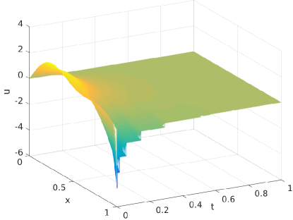
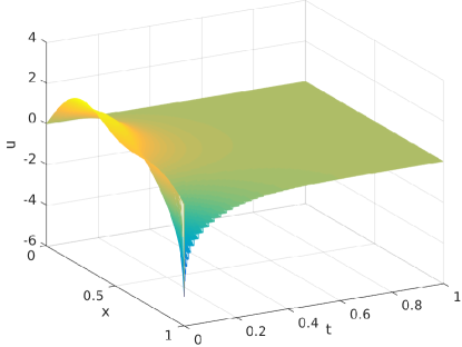
Figure 1: Numerical solutions of the closed-loop system (10)-(13) with $\theta=c=1$, $\lambda=\pi^{2}$, initial condition $u_{0}(x)=\sum_{n=1}^{3}\frac{\sqrt{2}}{n}\sin(n\pi x)+3(x^{2}-x^{3})$, $x\in[0,1]$ and under the event-triggered control (21)-(22). With $\beta=0.07$ in (21) the control updating is slower (closed-loop solution depicted on the left). With $\beta=0.02$ in (21), the control updating is faster (closed-loop solution depicted on the right).

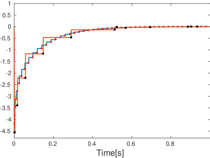
Figure 2: Time-evolution of the event-triggered boundary control (21)-(22) (orange line with black circle marker for slow control updating, i.e. $\beta=0.07$ in (21) and blue line with red circle marker for fast control updating, i.e. $\beta=0.02$ in (21)).

In addition, Figure 3 shows the time evolution of the functions appearing in the triggering condition (21) (on the left with $\beta=0.07$ and on the right with $\beta=0.02$). Once the trajectory $|d|$ reaches the trajectory $\beta\|k\|\|u[t]\|+\beta\|k\|\|u[t_{j}]\|$, an event is generated, the control value is updated and $d$ is reset to zero. It can be observed that the lower $\beta$ is, the faster the sampling and control updating which in turn implies smaller inter-executions times. This case turns out to be more conservative and the control function gets closer to the one in continuous case or even when considering a periodic scheme with a very small period. As a matter of fact, it is worth remarking that a sampling period can be computed from [15, Section 3.3]. Indeed, for the reaction-diffusion system with a boundary control whose actuation is done in a sampled-and-hold fashion, such a period would be $T=9.96\times 10^{-7}$. Notice that this is very small (even smaller than the time step discretization for the current simulations); consequently the periodic scheme turns out not be implementable. This is one of the reasons why event-triggered boundary control offers advantages with respect to periodic schemes. In our framework, the control value is updated aperiodically and only when needed.

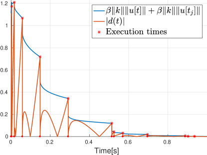
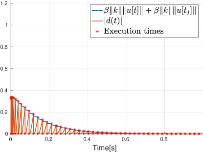
Figure 3: Trajectories involved in the triggering condition (21) (on the left with $\beta=0.07$ and on the right with $\beta=0.02$, resulting in slow and fast sampling, respectively). Once the trajectory $|d|$ reaches the trajectory $\beta\|k\|\|u[t]\|+\beta\|k\|\|u[t_{j}]\|$, an event is generated, the control value is updated and $d$ is reset to zero.

Finally, we run simulations for 100 different initial conditions given by $u_{0}(x)=\sum_{n=1}^{l}n^{2}\sqrt{2}\sin(n\pi x)+l(x^{2}-x^{3})$ for $l=1,..,10$ and $u_{0}(x)=\sum_{n=1}^{l}n\sqrt{2}\sin(n^{2}\pi x)+l(x^{2}-x^{3})$, for $l=11,...,100$ on a frame of $1s$. We have computed the inter-execution times between two triggering times. We compared the cases for slow and fast sampling, i.e. when $\beta=0.07$ and $\beta=0.02$, respectively. Figure 4 shows the density of the inter-execution times plotted in logarithmic scale where it can be observed that, the larger $\beta$ the less often is the sampling and control updating which in turn implies larger inter-executions times.

It is interesting to notice that when choosing $\beta$ small (resulting in fast sampling, as aforementioned), there are several inter-execution times of the order of $10^{-1.7}$ as depicted in blue bars in Figure 4 where the density predominates. It might suggest that a possible period (whenever one intends to sample periodically in a sampled-and-hold fashion) might be chosen with a length of the order $10^{-1.7}$. This issue is left for further tests and investigation with possible theoretical connections with periodic schemes as in [15]. This issue may give some hints on how to suitably choose sampling periods in order to reduce conservatism on periodic schemes.

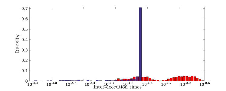
Figure 4: Density of the inter-execution times (logarithmic scale) computed for $100$ different initial conditions given by $u_{0}(x)=\sum_{n=1}^{l}n^{2}\sqrt{2}\sin(n\pi x)+l(x^{2}-x^{3})$ for $l=1,..,10$ and $u_{0}(x)=\sum_{n=1}^{l}n\sqrt{2}\sin(n^{2}\pi x)+l(x^{2}-x^{3})$, for $l=11,...,100$ on a frame of $1s$. With $\beta=0.07$ implying slow sampling and therefore larger inter-execution times (red bars) and with $\beta=0.02$ implying fast sampling and therefore smaller inter-execution times (blue bars).

5 Conclusion

In this paper, we have proposed an event-triggered boundary control to stabilize (on events) a reaction-diffusion PDE system with Dirichlet boundary condition. A suitable state-dependent event-triggering condition is considered. It determines when the control has to be updated. It has been proved the existence of a minimal dwell-time which is independent of the initial condition. Thus, it has been proved that there is no Zeno behavior and thus the well-posedness and the stability of the closed-loop system are guaranteed.

In future work, we may consider observer-based event-triggered control and possibly sampling output measurements on events as well. It may suggest that another event-triggered strategy shall be considered to be combined with the one for actuation. We expect also to address periodic event-triggered strategies inspired by some recent result from finite-dimensional systems [2]. For that, we may use the obtained dwell-time as a period or to come up with a maybe less conservative period. In either cases, the period would be utilized to monitor periodically the triggering condition while the actuation is still on events. This would represent even a more realistic approach toward digital realizations while reducing the consumption of computational resources.

References

- [1] G. Bastin and J.-M. Coron. Stability and Boundary Stabilization of 1-D Hyperbolic Systems. Birkhäuser Basel, 2016.
- [2] D.P. Borgers, R. Postoyan, A. Anta, P. Tabuada, D. Nešić, and W.P.M.H. Heemels. Periodic event-triggered control of nonlinear systems using overapproximation techniques. Automatica, 94:81 – 87, 2018.
- [3] R.M. Corless, G.H. Gonnet, D.E.G. Hare, D.J. Jeffrey, and D.E Knuth. On the Lambert W function. Advances in Computational Mathematics, 5:329–359, 1996.
- [4] MA. Davo, D. Bresch-Pietri, C Prieur, and F. Di Meglio. Stability analysis of a linear hyperbolic system with a sampled-data controller via backstepping method and looped-functionals. IEEE Transactions on Automatic Control, 2018.
- [5] N. Espitia, A. Girard, N. Marchand, and C Prieur. Event-based control of linear hyperbolic systems of conservation laws. Automatica, 70:275–287, August 2016.
- [6] N. Espitia, A. Girard, N. Marchand, and C. Prieur. Event-based stabilization of linear systems of conservation laws using a dynamic triggering condition. In Proc. of the 10th IFAC Symposium on Nonlinear Control Systems (NOLCOS), volume 49, pages 362–367, Monterey (CA), USA, 2016.
- [7] N. Espitia, A. Girard, N. Marchand, and C Prieur. Event-based boundary control of a linear 2x2 hyperbolic system via backstepping approach. IEEE Transactions on Automatic Control, 63(8):2686–2693, 2018.
- [8] E. Fridman and A. Blighovsky. Robust sampled-data control of a class of semilinear parabolic systems. Automatica, 48(5):826–836, 2012.
- [9] A. Girard. Dynamic triggering mechanisms for event-triggered control. IEEE Transactions on Automatic Control, 60(7):1992–1997, July 2015.
- [10] W.P.M.H. Heemels, K.H. Johansson, and P. Tabuada. An introduction to event-triggered and self-triggered control. In Proceedings of the 51st IEEE Conference on Decision and Control, pages 3270–3285, Maui, Hawaii, 2012.
- [11] L. Hetel, C. Fiter, H. Omran, A. Seuret, E. Fridman, J.-P. Richard, and SI. Niculescu. Recent developments on the stability of systems with aperiodic sampling: An overview. Automatica, 76:309 – 335, 2017.
- [12] A. Jiang, B. Cui, W. Wu, and B. Zhuang. Event-driven observer-based control for distributed parameter systems using mobile sensor and actuator. Computers & Mathematics with Applications, 72(12):2854 – 2864, 2016.
- [13] Z.-P Jiang, T. Liu, and P. Zhang. Event-triggered control of nonlinear systems: A small-gain paradigm. In 13th IEEE International Conference on Control Automation (ICCA), pages 242–247, July 2017.
- [14] I. Karafyllis and M. Krstic. Sampled-data boundary feedback control of 1-D Hyperbolic PDEs with non-local terms. Systems & Control Letters, 17:68–75, 2017.
- [15] I. Karafyllis and M. Krstic. Sampled-data boundary feedback control of 1-D parabolic PDEs. Automatica, 87:226 – 237, 2018.
- [16] I. Karafyllis and M. Krstic. Input-to-State Stability for PDEs. Springer-Verlag, London (Series: Communications and Control Engineering), 2019.
- [17] I. Karafyllis and M. Krstic. Small-gain-based boundary feedback design for global exponential stabilization of 1-d semilinear parabolic pdes. SIAM Journal on Control and Optimization, 57(3):2016–2036, 2019.
- [18] I. Karafyllis, M. Krstic, and K. Chrysafi. Adaptive boundary control of constant-parameter reaction–diffusion pdes using regulation-triggered finite-time identification. Automatica, 103:166–179, 2019.
- [19] M. Krstic and A. Smyshlyaev. Backstepping boundary control for first-order hyperbolic PDEs and application to systems with actuator and sensor delays. Systems & Control Letters, 57(9):750–758, 2008.
- [20] M. Krstic and A. Smyshlyaev. Boundary control of PDEs: A course on backstepping designs, volume 16. Siam, 2008.
- [21] M. Lemmon. Event-triggered feedback in control, estimation, and optimization. In Networked Control Systems, pages 293–358. Springer, 2010.
- [22] T. Liu and Z.-P. Jiang. A small-gain-approach to robust event-triggered control of nonlinear systems. IEEE Transaction on Automatic Control, 60(8):2072–2085, 2015.
- [23] H. Logemann, R. Rebarber, and S. Townley. Generalized sampled-data stabilization ofwell-posed linear infinite-dimensional systems. SIAM Journal on Control and Optimization, 44:1345–1369, 2005.
- [24] N. Marchand, S. Durand, and J. F. G. Castellanos. A general formula for event-based stabilization of nonlinear systems. IEEE Transactions on Automatic Control, 58(5):1332–1337, 2013.
- [25] R. Postoyan, P. Tabuada, D. Nešić, and A. Anta. A framework for the event-triggered stabilization of nonlinear systems. IEEE Transactions on Automatic Control, 60(4):982–996, 2015.
- [26] A. Selivanov and E. Fridman. Distributed event-triggered control of transport-reaction systems. Automatica, 68:344–351, 2016.
- [27] A. Seuret, S. Tarbouriech, C. Prieur, and L. Zaccarian. LQ-based event-triggered controller co-design for saturated linear systems. Automatica, 74:47–54, 2016.
- [28] A. Smyshlyaev and M. Krstic. Closed-form boundary state feedbacks for a class of 1-d partial integro-differential equations. IEEE Transactions on Automatic Control,, 49(12):2185–2202, Dec 2004.
- [29] P. Tabuada. Event-triggered real-time scheduling of stabilizing control tasks. IEEE Transactions on Automatic Control, 52(9):1680–1685, 2007.
- [30] Y. Tan, E. Trélat, Y. Chitour, and D. Nešić. Dynamic practical stabilization of sampled-data linear distributed parameter systems. In IEEE 48th Conference on Decision and Control (CDC), pages 5508–5513, 2009.
- [31] R. Vazquez, M. Krstic, and J.-M. Coron. Backstepping boundary stabilization and state estimation of a linear hyperbolic system. In the 50th IEEE Conference on Decision and Control and European Control Conference (CDC-ECC), pages 4937–4942, Orlando, United States, 2011.
- [32] Z. Yao and N.H. El-Farra. Resource-aware model predictive control of spatially distributed processes using event-triggered communication. In Proceedings of the 52nd IEEE Conference on Decision and Control, pages 3726–3731, Florence, Italy, 2013.
- [33] S. Yi, P.W. Nelson, and A.G. Ulsoy. Time-Delay Systems: Analysis and Control Using the Lambert W Function. World Scientific Publishing, Singapore, 2010.