Model-Agnostic Linear Competitors

Model-Agnostic Linear Competitors - When Interpretable Models Compete and Collaborate with Black-box Models

Hassan Rafique Program in Applied Mathematical and Computational Sciences (AMCS), University of Iowa, Iowa City, IA 52242, hassan-rafique@uiowa.edu

Tong Wang Tippie College of Business, University of Iowa, Iowa City, IA, 52245, tong-wang@uiowa.edu

Qihang Lin Tippie College of Business, University of Iowa, Iowa City, IA, 52245, qihang-lin@uiowa.edu

Driven by an increasing need for model interpretability, interpretable models have become strong competitors for black-box models in many real applications. In this paper, we propose a novel type of model where interpretable models compete and collaborate with black-box models. We present the Model-Agnostic Linear Competitors (MALC) for partially interpretable classification. MALC is a hybrid model that uses linear models to locally substitute any black-box model, capturing subspaces that are most likely to be in a class while leaving the rest of the data to the black-box. MALC brings together the interpretable power of linear models and good predictive performance of a black-box model. We formulate the training of a MALC model as a convex optimization. The predictive accuracy and transparency (defined as the percentage of data captured by the linear models) balance through a carefully designed objective function and the optimization problem is solved with the accelerated proximal gradient method. Experiments show that MALC can effectively trade prediction accuracy for transparency and provide an efficient frontier that spans the entire spectrum of transparency.

multi-class classification, interpretability, transparency

1 Introduction

With the rapid growth of data in volume, variety and velocity (Zikopoulos et al. 2012), there has been increasing need for modern machine learning models to provide accurate and reliable predictions and assist humans in decision making. The interaction of models and humans naturally calls for users’ understanding of machine learning models, especially in high-stake applications such as healthcare, judiciaries, etc (Letham et al. 2015, Yang et al. 2018, Caruana et al. 2015, Chen et al. 2018). Thus, many state-of-the-art machine learning models such as neural networks and ensembles stumble in these domains since they are black-box in nature. Black-box models have an opaque or highly complicated decision-making process that is hard for human to understand and rationalize. Driven by the practical needs, researchers have shifted their focus from only predictive performance driven to also account for transparency of models. It has recently been called by EU’s General Data Protection Regulation (GDPR) for the “right to explanation” (a right to information about individual decisions made by algorithms) (Parliament and of the European Union 2016, Phillips 2018) that requires human understandable predictive processes of models.

The recent advances in machine learning has seen an increasing amount of interest and work in interpretable machine learning, models and techniques that facilitate human understanding. Different forms of interpretable models have been developed, including rule-based models (Wang et al. 2017, Lakkaraju et al. 2017), scoring models (Zeng et al. 2017), case-based models (Richter and Weber 2016), etc. While these models can sometimes perform as well as black-box models, the performance loss is often inevitable, especially when the data is large and complex. This is because black-box models are optimized only for the predictive performance while interpretable models also pursue the small complexities. These two types of models have been competitors and mutally exclusive choices for users.

Another popular form of models have also risen quickly to assist human understandability, black-box explainers. Since the first paper of LIME (Ribeiro et al. 2016), a local linear explainer of any black-box model, various explainer models have been proposed (Ribeiro et al. 2018, Lundberg and Lee 2017). The main idea of explainers is they use simple and easily understandable models like decision rules or linear models, to locally or globally approximate the predictions of black-box models, providing “post-hoc” explanations with these simpler replica. However serious concerns have been brought up (Rudin 2019, Aïvodji et al. 2019, Thibault et al. 2019) on potential issues of black-box explainers since explainers only approximate but do not characterize exactly the decision-making process of a black-box model, often yielding an imperfect fidelity to the original black-box model. In addition, there exists ambiguity and inconsistency (Ross et al. 2017, Lissack 2016) in the explanation since there could be different explanations for the same prediction generated by different explainers, or by the same explainer with different parameters. There’s a very recent work that demonstrates that explanations can be deceptive and contrary to the real mechanism in a model (Aïvodji et al. 2019). Alvarez-Melis and Jaakkola (2018) showed LIME’s explanation of two close points (similar instances) can vary greatly. This is because LIME uses other instances in the neighborhood of the given instance to evaluate the local linear approximation. There are no clear guidelines for choosing an appropriate neighborhood that works the best and changing neighborhoods leads to a change in the explanations. This instability in the explanation demands a cautious and critical use of LIME. All of the issues result from the fact that the explainers only approximate in a post hoc way. They are not the decision-making process themselves.

In this paper, we propose a new form of model, which combines the intuitive power of interpretable models and the good predictive performance of black-box models, to reach some controllable middle ground where both transparency and good predictive performance is possible. The idea is simple and straightforward, a complex black-box model may have the best predictive performance overall, but it is not necessarily the best everywhere in the data space. Some instances may be accurately predicted by simpler models instead of the black-box model without losing any (or intolerable) predictive performance.

We design a unique mechanism where interpretable models complete and collaborate with a black-box model. Given a $K$ class classification problem, we design $K+1$ models, which we call agents. $K$ of the agents are interpretable, capturing $K$ classes, respectively. The remaining one is a pre-trained black-box model, called agent $\mathcal{B}$. Given an input $\mathbf{x}$, all of the $K$ agents bid to claim the input by proposing a score. The input is then assigned to the highest bidder with a significant margin over the other agents’ scores. If there does not exist a winner (not winning by a large margin), then none of the $K$ agents can claim the input, and it is then sent to agent $\mathcal{B}$ by default. At agent $\mathcal{B}$, the input will be classified, and this classification process is unknown to other agents the whole time, i.e., model-agnostic.

In this paper, we let all interpretable agents be linear models, which is one of the most popular forms of interpretable models. The black-box model can be any pre-trained multi-class classifier. We propose a model called Model-Agnostic Linear Competitors (MALC). MALC partitions the feature space into $K+1$ regions, each claimed by an agent. Agent $k(1\leq k\leq K)$ captures the most representative and confident characteristics of class $k$ by claiming the most plausible area for class $k$. Predictions for this area are inherently interpretable since the agents are linear models with regularized numbers of non-zero coefficients. The unclaimed area represents the subspace where none of the interpretable agents are very certain about, thus left to the most competent black-box agent $\mathcal{B}$. See Figure 1 for an illustration. Meanwhile, the coefficients of the $K$ linear models also show the most distinctive characteristics of each class, providing an intuitive description of the classes.

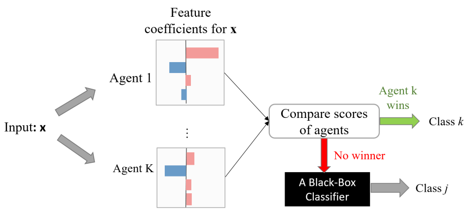
Figure 1: The decision-making process of MALC.

To train MACL, we formulate a carefully designed convex optimization problem which considers the predictive performance, interpretability of the linear agents (coefficients regularization), and most importantly, the percentage of the area claimed by the linear model, which we define as transparency of MALC. Then we use accelerated proximal gradient method (Nesterov 2013) to train MALC. By tuning the parameters, MACL can decide to send more or less area to the linear competitors, at the possible cost of the predictive performance.

Our work is differentiated from linear explainers such as Local Interpretable Model-agnostic Explainers (LIME) (Ribeiro et al. 2016), which provide post hoc approximations or explanations but do not participate in the predictive performance. Here our linear models directly compete with the black-box model to generate predictions, equivalent to locally substituting the black-box on a subset of data. Thus, MALC avoids some of the controversial issues of black-box explainers such as ambiguity and inconsistency in the explanations. In addition, LIME provides a local explanation for an instance while MACL characterizes a more global description of each class since it captures subspaces of classes.

The rest of the paper is organized as follows. We review related work in Section 2. The model is presented in Section 3, where we formulate the model and describe the training algorithm. We conduct an experimental evaluation in Section 4 on public datasets where MALC collaborates with state-of-the-art classifiers.

2 Related Work

Our work is related but different from recent black-box explainers. MALC does not explain or approximate the behavior of a black-box model, but instead, collaborates with the black-box model and shares the prediction task.

We have found a few works in the literature on the combination of multiple models (Kohavi 1996, Towell and Shavlik 1994). For example, (Kohavi 1996) combined a decision tree with a Naive Bayes model, (Shin et al. 2000) proposed a system combining neural network and memory-based learning, (Hua and Zhang 2006) combined SVM and logistic regression, etc. A recent work (Wang et al. 2015) divides feature spaces into regions with sparse oblique tree splitting and assign local sparse additive experts to individual regions. Besides these more isolated efforts, there has been a large body of continuous work on neural-symbolic or neural-expert systems (Garcez et al. 2015) pursued by a relatively small research community over the last two decades and has yielded several significant results (McGarry et al. 1999, Garcez et al. 2012, Taha and Ghosh 1999, Towell and Shavlik 1994). This line of research has been carried on to combine deep neural networks with expert systems to improve predictive performance (Hu et al. 2016).

Compared to the models discussed above, our method is distinct in that it is model-agnostic and can work with any black-box classifier. The black-box can be a carefully calibrated, advanced model using confidential features or techniques. Our model only needs predictions from the black-box and does not need to alter the black-box during training or know any other information from it. This minimal requirement of information from the black-box collaborator renders much more flexibility in creating collaboration between different models, largely preserving confidential information from the more advanced partner.

One work that’s closest to ours is Hybrid Rule Sets (HyRS) (Wang 2019) that builds a hybrid of decision rules and a black-box model. An input goes through a positive rule set, a negative rule set, and a black-box model sequentially until it is classified by the first model that captures it. HyRS produce interpretable predictions on instances captured by rules. A HyRS only works with binary classification. MALC, on the other hand, can work with multi-class classification. The $K$ interpretable agents compete for an input simultaneously in a fair mechanism.

3 Model-Agnostic Linear Competitors

In this paper, we focus on the multi-class classification problem. Suppose there are $K$ distinct classes. We consider an approach similar to one-vs-all linear classification. We us review how this classification works. Given a linear classifier $f_{i}(\mathbf{x})=\mathbf{w}^{\top}_{i}\mathbf{x}$, $i\in[K]:=\{1,2,...,K\}$, if $f_{i}(\mathbf{x})-f_{j}(\mathbf{x})\geq 0$, for every $j$ other than $i$, then $\mathbf{x}$ belongs to class $i$. For class $i$,

$$\mathcal{P}_{i}(\mathbf{x})=\bigcap_{j\not=i}\bigg{\{}f_{i}(\mathbf{x})-f_{j}(\mathbf{x})=0\bigg{\}}$$

is the decision boundary. Most mistakes made by a linear model happen around the decision boundary. Therefore, in a hybrid model, we exploit the high predictive power of a black-box model and leave this more difficult area to it while having the linear classifier classify the rest. Then the linear classifier produces a decision only when it is confident enough, this time comparing against thresholds $\{\theta_{i}\geq 0\}^{K}_{i=1}$: to predict class $i$ when $f_{i}(\mathbf{x})-f_{j}(\mathbf{x})\geq\theta_{i}$ for every $j$ other than $i$ and unclassified otherwise. Thus the linear model generates $K$ decision boundaries, creating a partition of a data space into $K+1$ regions, a region for each of the $K$ classes and an unclassified region. This unclassified region contains data that the linear model is not confident to decide so that black-box is activated to generate predictions., see Figure 2. Thus we build $K$ linear competitors, each advocating for a class, to collaborate with the black-box model. We call this classification method Model-Agnostic Linear Competitors (MALC) model.

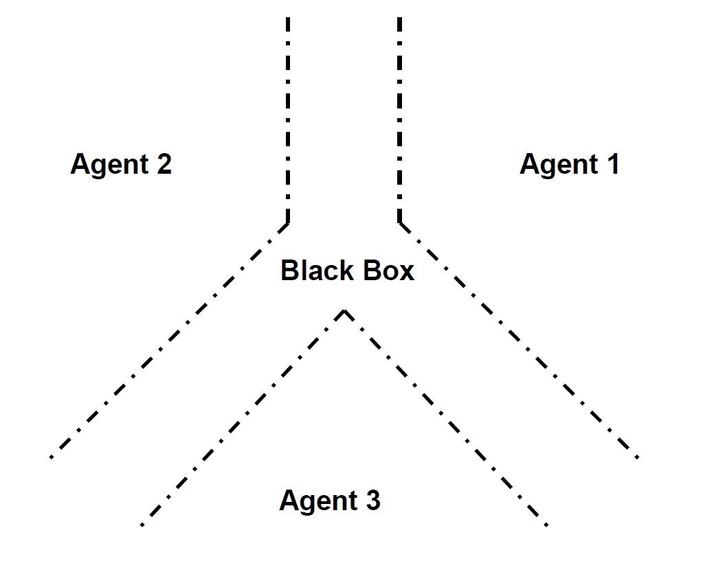
Figure 2: A simplified depiction of partitioning of the data space in the case of three classes, by linear and black-box agents.

The goal of building such a collaborative linear model is to replace the black-box system with a transparent system on a subset of data, at the minimum loss of predictive accuracy. Therefore a key determinant in the success of MALC is the partitioning of the data, which is determined by the coefficients $\mathbf{w}_{i}$ in the linear model and the thresholds $\theta_{i}$, $i\in[K]$. In this paper, we formulate a convex optimization problem to learn the coefficients and thresholds. The objective function considers the fitness to the training data, captured by a convex loss function, the regularization term, and the sum of thresholds. As $\theta_{i}$ gets close to $0$, more data can be decided by the linear model, increasing the transparency of the decision-making process, but at the cost of possible loss of predictive performance. Our formulation is compatible with various forms of convex loss function and guarantees global optimality.

We work with a set of training examples $\mathcal{D}=\{(\mathbf{x}_{i},y_{i})\}_{i=1}^{n}$ where $\mathbf{x}_{i}\in\mathbb{R}^{d}$ is a vector of $d$ attributes and $y_{i}\in[K]:=\{1,2,...,K\}$ is the corresponding class label. Let $f(\mathbf{x}):\mathbb{R}^{d}\rightarrow[K]$ represent the MALC classification model that is constructed based on linear models $f_{l,i}(\mathbf{x})=\mathbf{w}^{\top}_{i}\mathbf{x}$, $i\in[K]$ and a black-box model $f_{b}(\mathbf{x}):\mathbb{R}^{d}\rightarrow[K]$. The black-box model is given, which can be any trained model. We need its prediction on the training data $\mathcal{D}$, denoted as $\{y^{b}_{i}\}_{i=1}^{n}$ and $y^{b}_{i}=f_{b}(\mathbf{x}_{i})$. Our goal is to learn the coefficients $\mathbf{w_{i}}$ in the linear models $f_{l,i}$ together with thresholds $\theta_{i}$ ( $\geq 0$), $i\in[K]$, in order to form a hybrid decision model $f$ as:

$$f(\mathbf{x})=\left\{\begin{array}[]{cl}k&\text{ if }\mathbf{w}_{k}^{\top}\mathbf{x}-\mathbf{w}_{j}^{\top}\mathbf{x}\geq\theta_{k},~{}k\in[K],~{}\forall~{}j\in[K]\setminus\{k\}\\ f_{b}(\mathbf{x})&~{}\text{otherwise}\end{array}\right.$$ (3)

Note the hybrid model uses $K$ thresholds to partition the data space into $K+1$ regions, a region for each class and an undetermined region left to the black-box model. Data that falls into any of the $K$ class’s claimed regions is considered “transparent” by the linear model, and we refer to the percentage of this data subset as the transparency of the model.

3.1 Model Formulation

In this section, we formulate an optimization framework to build a MALC model. We consider three factors when building the model: predictive performance, data transparency, and model regularization. We elaborate each of them below.

The (in-sample) predictive performance characterizes the fitness of the model to the training data. Since $f_{b}$ is pre-given, the predictive performance is determined by two factors, the accuracy of $f_{l}=[f_{l,1},~{}f_{l,2},...~{},f_{l,K}]$ on instances as described in (3) and the accuracy of $f_{b}$ on the remaining examples. We wish to obtain a good partition of data $\mathcal{D}$ by assigning $f_{b}$ and $f_{l}$ to a different region of the data such that the strength of $f_{b}$ and $f_{l}$ are properly exploited. Second, we include the sum $\sum\theta_{i}$ as a penalty term in the objective to account for data transparency of the hybrid model. The smaller sum implies more data is classified by the linear model. In the most extreme case where $\sum\theta_{i}=0$, all data is sent to the linear model, and the MALC model is reduced to a pure one-vs all linear classifier, i.e., transparency equals one. Finally, we also need to consider model regularization in the objective. As the weight for the sparsity enforcing regularization term increases, the model encourages using a smaller number of features which increases the interpretability of the model as well as preventing overfitting.

Combining the three factors discussed above, we formulate the learning objective for MALC as:

$$F^{*}:=\min_{\mathbf{w},\theta\geq 0}\left\{F(\mathbf{w},\theta):=\mathcal{L}(\mathbf{w},\theta;\mathcal{D})+C_{1}\sum^{K}_{i=1}\theta_{i}+C_{2}r(\mathbf{w})\right\},$$ (4)

where $\mathbf{w}=[\mathbf{w}_{1},~{}\mathbf{w}_{2},...~{},\mathbf{w}_{K}]$, $\mathbf{\theta}=[\theta_{i},~{}\theta_{2},...~{},\theta_{K}]$, $\mathcal{L}(\mathbf{w},\theta;\mathcal{D})$ is the loss function defined on the training set $\mathcal{D}$ associated to the decision rule $f$ in (3), $\sum^{K}_{i=1}\theta_{i}$ is a penalty term to increase the transparency of $f$, $r$ is a convex and closed regularization term (e.g. $\|\mathbf{w}\|_{1}$, $\frac{1}{2}\|\mathbf{w}\|_{2}^{2}$ or an indicator function of a constraint set), and $C_{1}$ and $C_{2}$ are non-negative coefficients which balance the importance of the three components in (4).

Let $I_{k}=\{i~{}|~{}y_{i}=k\}$, which is the index set of all the data points $(\mathbf{x})$ belonging to class $k$. Similarly, let $I^{+}_{k}=\{i\in I_{k}~{}|~{}y^{i}_{b}=y_{i}\}$ and $I^{-}_{k}=\{i\in I_{k}~{}|~{}y^{i}_{b}\not=y_{i}\}$. The loss function in (4) over the dataset $\mathcal{D}$ is then defined as

$$\mathcal{L}(\mathbf{w},\mathbf{\theta};\mathcal{D})=\frac{1}{n}\sum^{K}_{k=1}\sum_{i\in I^{+}_{k}}\sum^{K}_{j=1\atop j\not=k}\phi(\mathbf{w}_{k}^{\top}\mathbf{x}_{i}-\mathbf{w}_{j}^{\top}\mathbf{x}_{i}+\theta_{j})+\frac{1}{n}\sum^{K}_{k=1}\sum_{i\in I^{-}_{k}}\sum^{K}_{j=1\atop j\not=k}\phi(\mathbf{w}_{k}^{\top}\mathbf{x}_{i}-\mathbf{w}_{j}^{\top}\mathbf{x}_{i}-\theta_{k})$$ (5)

where function $\phi(z):\mathbb{R}\rightarrow\mathbb{R}$ is a non-increasing convex closed loss function which can be one of those commonly used in linear classification such as the hinge loss $\phi(z)=(1-z)_{+}$, smooth hinge loss $\phi(z)=\frac{1}{2}(1-z)^{2}_{+}$ or the logistic loss $\phi(z)=\log(1+\exp(-z))$. Note that $\{I_{k}=I^{+}_{k}\cup I^{-}_{k}\}^{K}_{k=1}$ form a partition of $\{1,2,\dots,n\}$. The intuition of this loss function is as follows. Take a data point $\mathbf{x}_{i}$ with $y_{i}=k$ and $y^{b}_{i}=k$ as an example. Our hybrid model (3) will classify $\mathbf{x}_{i}$ correctly as long as it does not fall into the region of a class other than $k$. To ensure $\mathbf{x}_{i}$ does not fall into another class’s region, we need $\mathbf{w}^{\top}_{j}\mathbf{x}_{i}-\mathbf{w}^{\top}_{k}\mathbf{x}_{i}<\theta_{j}$ for every $j$ other than $k$. Hence, with the non-increasing property of $\phi$, the loss term $\phi(\mathbf{w}_{k}^{\top}\mathbf{x}_{i}-\mathbf{w}_{j}^{\top}\mathbf{x}_{i}+\theta_{j})$ will encourage a positive value of $\mathbf{w}_{k}^{\top}\mathbf{x}_{i}-\mathbf{w}_{j}^{\top}\mathbf{x}_{i}+\theta_{j}$ which means we have $\mathbf{w}_{j}^{\top}\mathbf{x}_{i}-\mathbf{w}_{k}^{\top}\mathbf{x}_{i}<\theta_{j}$. On the other hand, for a data point $\mathbf{x}_{i}$ with $y_{i}=k$ and $y^{b}_{i}\not=k$, our hybrid model will classify $\mathbf{x}_{i}$ correctly only when $\mathbf{x}_{i}$ falls in the class $k$ region, namely, $\mathbf{w}^{\top}_{k}\mathbf{x}_{i}-\mathbf{w}^{\top}_{j}\mathbf{x}_{i}\geq\theta_{k}$ for every $j$ other than $k$. Hence, we use the loss term $\phi(\mathbf{w}_{k}^{\top}\mathbf{x}_{i}-\mathbf{w}_{j}^{\top}\mathbf{x}_{i}-\theta_{k})$ to encourage a positive value of $\mathbf{w}_{k}^{\top}\mathbf{x}_{i}-\mathbf{w}_{j}^{\top}\mathbf{x}_{i}-\theta_{k}$.

3.2 Model Training

With the loss function defined in (5), the hybrid model can be trained by solving the convex minimization problem (4) for which many efficient optimization techniques are available in literature including subgradient methods (Nemirovski et al. 2009, Duchi et al. 2011), accelerated gradient methods (Nesterov 2013, Beck and Teboulle 2009), primal-dual methods (Nemirovski 2004, Chambolle and Pock 2011) and many stochastic first-order methods based on randomly sampling over coordinates or data (Johnson and Zhang 2013, Duchi et al. 2011). The choice of algorithms for (4) depends on various characteristics of the problem such as smoothness, strong convexity, and data size.

Since numerical optimization is not the focus of this paper, we will simply utilize the accelerated proximal gradient method (APG) by Nesterov (Nesterov 2013) to solve (4) when $\phi$ is smooth.

4 Experiments

We perform a detailed experimental evaluation of the proposed model on four public datasets. The goal here is to examine the predictive performance, the transparency, and the model complexity. In addition, we characterize the trade-off between predictive accuracy and transparency using efficient frontiers. To do that, we vary the parameters $C_{1}$ and $C_{2}$ to generate a list of models producing an accuracy-transparency curve for each dataset. We also analyze a medical dataset in detail to provide users more intuitive understanding of the model.

Datasets

We analyze four real-world datasets that are publicly available at (Chang and Lin 2011, Ilangovan 2017, Quinlan et al. 1986, Wang et al. 2017). 1) Coupon (Wang et al. 2017) (12079 $\times$ 113) studies responses of consumers to recommendation of coupons when users are driving in different contexts, using feature such as the passenger, destination, weather, time, etc. The three classes are “decline”, ”accept and will use right away”, and “accept and will use later” 2) Covtype(Chang and Lin 2011) (581,012 $\times$ 54) studies the forest cover type of wilderness areas which include Roosevelt National Forest of northern Colorado. There are seven different forest cover types. The features in the covtype dataset are scaled to $[0,1]$. 3) Thyroid(Quinlan et al. 1986) (9172 $\times$ 63) studies the prediction of thyroid diagnoses based on patients’ biomedical information. 4) Medical (Ilangovan 2017) (106,643 $\times$ 14) provide information about Clinical, Anthropometric and Biochemical (CAB) survey done by Govt. of India. This survey was conducted in nine states of India with a high rate of maternal and infant death rates in the country. We focused on the subset of data for children under the age of five and predicted their illness type. We dropped some features not needed for classification, and the missing values in certain features were replaced by mean or mode values appropriately. For each dataset, we randomly sample 80% instances to form the training sets and use the remaining 20% as the testing sets. Since the Medical dataset is highly unbalanced among different classes, we downsample the majority class and upsample the minority class to make them balanced.

Training Black-box Models

We first choose three state-of-the-art black-box classifiers, Random Forest (Liaw et al. 2002), XGBoost (Chen and Guestrin 2016) and fully-connected neural network with two hidden layers. All of these models are implemented with R. The Random Forest model is built using the ranger package (Wright and Ziegler 2015). The XGBoost model is built using the xgboost package (Chen et al. 2015). The neural network model is built using the keras package (Chollet and Allaire 2017). For each model, we identify one or two hyperparameters and, for each dataset, we apply an $80\%$-$20\%$ holdout method on the training set to select the values for these hyperparameters from a discrete set of candidates that give the best validation performance. For Random Forest, we use $500$ trees and tune the minimum node size and maximal tree depth. For XGBoost, we tune maximal tree depth and the number of boosting iterations. For the neural network, we choose the sigmoid function to be the activation function and tune the number of neurons and the dropout rates in the two hidden layers.

Training MALC

We use the predictions of the three black-box models on the training set as the input to build MALC models. In (4), we choose $\phi$ to be the smooth hinge loss and $r(\mathbf{w})=\|\mathbf{w}\|_{1}$. We would like to obtain a list of models that span the entire spectrum of transparency, so we vary $C_{1}$ and $C_{2}$ to achieve that goal. Note that $C_{1}$ is directly related to transparency, and we use grid-search to find a suitable range to achieve transparency from zero to one. $C_{2}$ is related to the sparsity of the model. Overall, we choose $C_{1}$ from $[0.005,0.95]$ and $C_{2}$ from $[0.03,0.25]$. For each $C_{1}$ value, we use $80\%$-$20\%$ holdout on the training set to choose $C_{2}$ from a discrete set of candidates that give the best validation performance. After choosing the pairs of $(C_{1},C_{2})$ values, the Algorithm APG is run up to $10,000$ iterations to make sure the change in objective value was less than $0.1\%$, in the last iterations, to ensure the convergence.

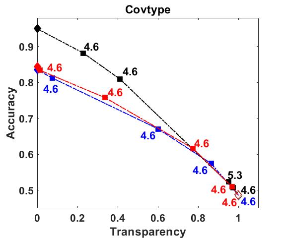
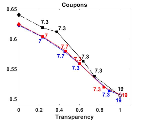
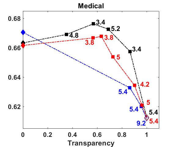
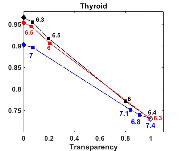
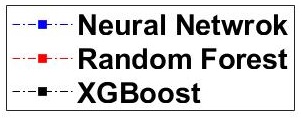
Figure 3: The efficient frontiers of MALC when collaborating with different black-box models. The numbers represent the average number of features being used by the MALC model.

Efficient Frontier Analysis

In Figure 3, each efficient frontier starts with a transparency value of zero, which corresponds to a pure black-box model. The general trend is as transparency increases, accuracy tends to decrease. The medical dataset provides an interesting scenario where the initial increase in transparency does not lead to a decrease in predictive performance. The rate of change of transparency w.r.t predictive performance is different for each dataset. For Thyroid dataset, the accuracy decreases almost linearly, whereas, for coupon and covtype datasets, accuracy decreases steadily as the transparency increases. However, for the medical dataset, the accuracy does not decrease initially and then falls significantly after a certain transparency threshold. Note that the transparency value of one corresponds to a pure linear (interpretable) model. But the interpretability comes at a huge cost of predictive performance, as evident by considerably low accuracy of linear models compared to the accuracy of the black-box models for all datasets. MALC provides the user with a unique framework of choosing a model from the whole spectrum of options available on an efficient frontier with their desired accuracy and transparency. We recommend the users to choose the models around the tipping point to ensure gain in transparency without a significant loss in accuracy.

Number of Features Analysis

We would also like to make sure the linear models are indeed interpretable, i.e., using a few non-zero terms in the model. We report in Figure 3 the average number of non-zero coefficients in MALC, which is calculated as a ratio of the number of non-zero coefficients in $K$ linear models ($\mathbf{w}$) to the number of classes in the dataset. Observe that MALC models require a relatively small number of features from the dataset to gain transparency, preserving the interpretability of linear models.

The control over transparency-accuracy trade-off and use of a small number of features to gain transparency make MALC a strong candidate for real-world applications, particularly when the user wants to avoid the black-box methods.

4.1 Case Study on the Medical Dataset

We show an example of MALC on the medical dataset. There are a total of five classes in this datsaet, “no illness”, diarrhea/dysentery”, “acute respiratory infection”, “fever of any type”, and “other illness”. MALC was built in collaboration with a pre-trained random forest whose accuracy is 66.0%. After building five linear competitors, the accuracy of MALC reaches 66.4% while gaining transparency of 77.7%. The coefficients of the five linear models are shown in Figure 4. From the linear models, one can easily extract some of the key characteristics for each class. For example, the later children start to receive semisolid food and the longer they are exclusively breastfed (feature “day_or_month_for_breast_feeding )”, the more likely they will be free of any of the illness (Class 1). Children who start receiving semisolid mashed food (feature “semisolid_month_or_day”) at a very young age, start receiving water at an early age (feature “water_month”), and are too late to start receiving animal milk/formula milk (feature “ani_milk_month”) are more likely to have acute respiratory infection (Class 3).

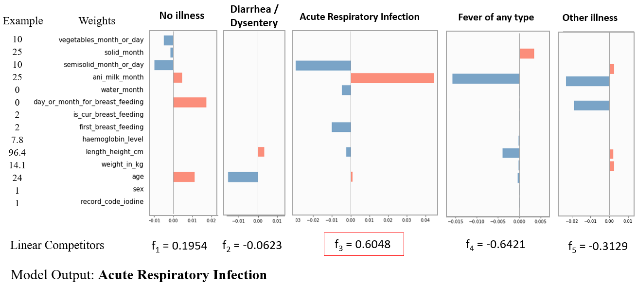
Figure 4: An example of MALC in collaboration with a pre-trained random forest

We chose an example instance and show the input features and the output of the linear models in Figure 4. This child started receiving animal milk/formula milk at age of $25$ months, almost six times of the average age of receiving animal/formula milk (4.3 months). This child started receiving semisolid food at 10 months old, later than the average age of children (5.8 months) who start receiving semisolid food. This is helpful for the child’s overall health conditions as suggested by classifier 1. However, this effect is completely overtaken by the late usage of formula milk.

In addition, the child was breast fed later than $64\%$ of the children in the dataset. Combining these important features, classifier 3 outputs the highest score, with a large enough margin over the other four linear models. Thus this child is predicted to have acute respiratory infection, which is consistent with the true label.

An interesting observation for this model is it performs slightly better than the black-box alone, which means the 77.7% transparency is obtained for free. This is the desired situation for hybrid models like MALC to be adopted.

4.2 Comparison with baselines

There are two lines of work in interpretable machine learning, stand-alone interpretable models like decision trees and black-box explainers like LIME. MACL has a unique model form does not fall into either of them. We choose representative models from each category. We compare with three decision trees as stand-alone interpretable models and LIME as an explainer. We focus and present results on the medical data. First, comparison with decision trees show that interpretable models are insufficiant for this dataset since they generate lower accuracy. In addition, we report the size of trees represented by the number of nodes in a tree to quantify the model complexity. Decision trees have significantly larger model sizes, as reported in Table 1.

Table 1: Performance comparison with baseline models

	MALC	CART	C4.5	C5.0
accuracy	0.66	0.63	0.63	0.62
# of rules	–	84	46	67
# of conditions	26 non-zero coefficients from 5 linear models	167	91	132

For comparison with LIME, we sample up to $200$ examples from each of the five classes that are explained by one of the linear classifiers in MALC and use LIME to generate explanations for each of them. We observe two issues with LIME. First, the inter-class explanations of LIME are too similar, as shown by the mean and std of the coefficients of LIME in Figure 5: the means of are almost identical across classes. This makes it difficult for users to understand the difference between classes and it’s hard to use the explanations to reason why an instance is classified into a particular class but not others. Unlike LIME, MALC provides different coefficients for different classes (see Figure 4) so that users can easily understand what features differentiate one class from the others.

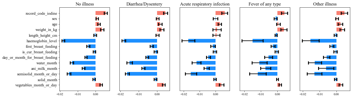
Figure 5: Means and Standard Deviations of Coefficients of LIME

Second, Alvarez-Melis and Jaakkola (2018) showed that LIME’s explanation of two close (similar) instances can vary greatly. This is because LIME uses other instances in the neighborhood of the given instance to evaluate the local linear approximation. There are no clear guidelines for choosing an appropriate neighborhood that works the best and changing neighborhoods leads to a change in the explanations. This instability in the explanation demands a cautious and critical use of LIME. On the other hand, MALC provides a set of global linear models and is relatively independent of the local neighborhood. This means that explanations provided by MALC are more consistent and stable.

5 Conclusion

We proposed a Model-Agnostic Linear Competitors (MALC) model for multi-class classification. MALC builds $K$ linear models to collaborate with a pre-trained black-box model. The data space is partitioned by MALC, into regions classified by the linear model and the black-box with linear decision boundaries. We formulated the training of a MALC model as convex optimization, where predictive accuracy and transparency balance through objective function. The optimization problem is solved with the accelerated proximal gradient method.

MALC is model-agnostic, which makes it flexible to collaborate with any black-box model, needing only their predictions on the dataset. In this paper, MALC collaborated with Random Forest, XGBoost, and Neural Networks to solve multiclass classification problems. Experiments show that MALC was able to yield models with different transparency and accuracy values by varying the parameters, thus providing more model options to users. In real applications, users can decide the operating point based on the efficient frontier. The decision will depend on knowing how much loss in accuracy is tolerable and how much transparency is desired in their application.

Compared to post hoc black-box explainers such as LIME, the linear models in MALC are predictive models, which guarantee 100% fidelity on data that are claimed by them. Also, unlike linear explainers that provide local explanations, the linear models in MALC capture global characteristics of classes by building $K$ linear models at the same time to compete with each other. Thus the coefficients learned are often the most distinguishing features.

The proposed work offers a new perspective in building handshakes between interpretable and black-box models, in addition to using the former as the post hoc analysis to the latter in the current literature. Here we propose to build collaboration between the two to exploit the strength of both. Despite the difference in the goal, existing black-box model explainers such as LIME can still be applied to explain the subset of data sent to the black-box.

References

- Aïvodji et al. (2019) Aïvodji, Ulrich, Hiromi Arai, Olivier Fortineau, Sébastien Gambs, Satoshi Hara, Alain Tapp. 2019. Fairwashing: the risk of rationalization. International Conference on Machine Learning .
- Alvarez-Melis and Jaakkola (2018) Alvarez-Melis, David, Tommi S. Jaakkola. 2018. On the robustness of interpretability methods. ICML Workshop on HumanInterpretability in Machine Learning .
- Beck and Teboulle (2009) Beck, Amir, Marc Teboulle. 2009. A fast iterative shrinkage-thresholding algorithm for linear inverse problems. SIAM journal on imaging sciences 2(1) 183–202.
- Caruana et al. (2015) Caruana, Rich, Yin Lou, Johannes Gehrke, Paul Koch, Marc Sturm, Noemie Elhadad. 2015. Intelligible models for healthcare: Predicting pneumonia risk and hospital 30-day readmission. Proceedings of the 21th ACM SIGKDD International Conference on Knowledge Discovery and Data Mining. ACM, 1721–1730.
- Chambolle and Pock (2011) Chambolle, Antonin, Thomas Pock. 2011. A first-order primal-dual algorithm for convex problems with applications to imaging. Journal of mathematical imaging and vision 40(1) 120–145.
- Chang and Lin (2011) Chang, Chih-Chung, Chih-Jen Lin. 2011. LIBSVM: A library for support vector machines. ACM Transactions on Intelligent Systems and Technology 2 27:1–27:27. Software available at http://www.csie.ntu.edu.tw/~cjlin/libsvm.
- Chen et al. (2018) Chen, Chaofan, Kangcheng Lin, Cynthia Rudin, Yaron Shaposhnik, Sijia Wang, Tong Wang. 2018. An interpretable model with globally consistent explanations for credit risk. arXiv preprint arXiv:1811.12615 .
- Chen et al. (2015) Chen, T., M. Benesty, V. Khotilovich, Y. Tang. 2015. Xgboost: extreme gradient boosting. R package version 0.4.
- Chen and Guestrin (2016) Chen, Tianqi, Carlos Guestrin. 2016. Xgboost: A scalable tree boosting system. Proceedings of the 22nd acm sigkdd international conference on knowledge discovery and data mining. ACM, 785–794.
- Chollet and Allaire (2017) Chollet, F., J. Allaire. 2017. R interface to keras. Retrieved from https://github.com/rstudio/keras.
- Duchi et al. (2011) Duchi, John, Elad Hazan, Yoram Singer. 2011. Adaptive subgradient methods for online learning and stochastic optimization. Journal of Machine Learning Research 12(Jul) 2121–2159.
- Garcez et al. (2015) Garcez, A d’Avila, Tarek R Besold, Luc De Raedt, Peter Földiak, Pascal Hitzler, Thomas Icard, Kai-Uwe Kühnberger, Luis C Lamb, Risto Miikkulainen, Daniel L Silver. 2015. Neural-symbolic learning and reasoning: contributions and challenges. Proceedings of the AAAI Spring Symposium on Knowledge Representation and Reasoning: Integrating Symbolic and Neural Approaches, Stanford.
- Garcez et al. (2012) Garcez, Artur S d’Avila, Krysia B Broda, Dov M Gabbay. 2012. Neural-symbolic learning systems: foundations and applications. Springer Science & Business Media.
- Hu et al. (2016) Hu, Zhiting, Xuezhe Ma, Zhengzhong Liu, Eduard Hovy, Eric Xing. 2016. Harnessing deep neural networks with logic rules. arXiv preprint arXiv:1603.06318 .
- Hua and Zhang (2006) Hua, Zhongsheng, Bin Zhang. 2006. A hybrid support vector machines and logistic regression approach for forecasting intermittent demand of spare parts. Applied Mathematics and Computation 181(2) 1035–1048.
- Ilangovan (2017) Ilangovan, Rajanand. 2017. Clinical, anthropometric & bio-chemical survey. Retrieved from https://www.kaggle.com/rajanand/cab-survey.
- Johnson and Zhang (2013) Johnson, Rie, Tong Zhang. 2013. Accelerating stochastic gradient descent using predictive variance reduction. Advances in neural information processing systems. 315–323.
- Kohavi (1996) Kohavi, Ron. 1996. Scaling up the accuracy of naive-bayes classifiers: A decision-tree hybrid. KDD, vol. 96. 202–207.
- Lakkaraju et al. (2017) Lakkaraju, Himabindu, Ece Kamar, Rich Caruana, Jure Leskovec. 2017. Interpretable & explorable approximations of black box models. arXiv preprint arXiv:1707.01154 .
- Letham et al. (2015) Letham, Benjamin, Cynthia Rudin, Tyler H McCormick, David Madigan, et al. 2015. Interpretable classifiers using rules and bayesian analysis: Building a better stroke prediction model. The Annals of Applied Statistics 9(3) 1350–1371.
- Liaw et al. (2002) Liaw, Andy, Matthew Wiener, et al. 2002. Classification and regression by randomforest. R news 2(3) 18–22.
- Lissack (2016) Lissack, M. 2016. Dealing with ambiguity–the ‘black box’as a design choice. SheJi (forthcoming) .
- Lundberg and Lee (2017) Lundberg, Scott M, Su-In Lee. 2017. A unified approach to interpreting model predictions. Advances in Neural Information Processing Systems. 4768–4777.
- McGarry et al. (1999) McGarry, Kenneth, Stefan Wermter, John MacIntyre. 1999. Hybrid neural systems: from simple coupling to fully integrated neural networks. Neural Computing Surveys 2(1) 62–93.
- Nemirovski (2004) Nemirovski, Arkadi. 2004. Prox-method with rate of convergence for variational inequalities with lipschitz continuous monotone operators and smooth convex-concave saddle point problems. SIAM Journal on Optimization 15(1) 229–251.
- Nemirovski et al. (2009) Nemirovski, Arkadi, Anatoli Juditsky, Guanghui Lan, Alexander Shapiro. 2009. Robust stochastic approximation approach to stochastic programming. SIAM Journal on optimization 19(4) 1574–1609.
- Nesterov (2013) Nesterov, Yurii. 2013. Introductory lectures on convex optimization: A basic course, vol. 87. Springer Science & Business Media.
- Parliament and of the European Union (2016) Parliament, Council of the European Union. 2016. General data protection regulation.
- Phillips (2018) Phillips, Mark. 2018. International data-sharing norms: from the oecd to the general data protection regulation (gdpr). Human genetics 1–8.
- Quinlan et al. (1986) Quinlan, J. Ross, Paul Compton, K. A. Horn, Lloyd Lazarus. 1986. Inductive knowledge acquisition: a case study. In Proceedings of the second Australian Conference on the Applications of Expert Systems. 183–204.
- Ribeiro et al. (2016) Ribeiro, Marco Tulio, Sameer Singh, Carlos Guestrin. 2016. Why should i trust you?: Explaining the predictions of any classifier. Proceedings of the 22nd ACM SIGKDD International Conference on Knowledge Discovery and Data Mining. ACM, 1135–1144.
- Ribeiro et al. (2018) Ribeiro, Marco Tulio, Sameer Singh, Carlos Guestrin. 2018. Anchors: High-precision model-agnostic explanations. Thirty-Second AAAI Conference on Artificial Intelligence.
- Richter and Weber (2016) Richter, Michael M, Rosina O Weber. 2016. Case-based reasoning. Springer.
- Ross et al. (2017) Ross, Andrew Slavin, Michael C Hughes, Finale Doshi-Velez. 2017. Right for the right reasons: Training differentiable models by constraining their explanations. arXiv preprint arXiv:1703.03717 .
- Rudin (2019) Rudin, Cynthia. 2019. Stop explaining black box machine learning models for high stakes decisions and use interpretablemodels instead. Nature Machine Intelligence 180 206–215.
- Shin et al. (2000) Shin, Chung-Kwan, Ui Tak Yun, Huy Kang Kim, Sang Chan Park. 2000. A hybrid approach of neural network and memory-based learning to data mining. IEEE Transactions on Neural Networks 11(3) 637–646.
- Taha and Ghosh (1999) Taha, Ismail A, Joydeep Ghosh. 1999. Symbolic interpretation of artificial neural networks. IEEE Transactions on knowledge and data engineering 11(3) 448–463.
- Thibault et al. (2019) Thibault, Laugel, Lesot Marie-Jeanne, Marsala Christophe, Renard Xavier, Marcin Detyniecki. 2019. The dangers of post-hoc interpretability:unjustified counterfactual explanations. Proceedings of the Twenty-Eighth International Joint Conference on Artificial Intelligence .
- Towell and Shavlik (1994) Towell, Geoffrey G, Jude W Shavlik. 1994. Knowledge-based artificial neural networks. Artificial intelligence 70(1-2) 119–165.
- Wang et al. (2015) Wang, Jialei, Ryohei Fujimaki, Yosuke Motohashi. 2015. Trading interpretability for accuracy: Oblique treed sparse additive models. SIGKDD. ACM, 1245–1254.
- Wang (2019) Wang, Tong. 2019. Gaining no or low-cost transparency with interpretable partial substitute. International Conference on Machine Learning .
- Wang et al. (2017) Wang, Tong, Cynthia Rudin, F Doshi, Yimin Liu, Erica Klampfl, Perry MacNeille. 2017. A bayesian framework for learning rule set for interpretable classification. Journal of Machine Learning Research .
- Wright and Ziegler (2015) Wright, Marvin N., Andreas Ziegler. 2015. ranger: A fast implementation of random forests for high dimensional data in c++ and r. arXiv preprint arXiv:1508.04409.
- Yang et al. (2018) Yang, Carl, Xiaolin Shi, Luo Jie, Jiawei Han. 2018. I know you’ll be back: Interpretable new user clustering and churn prediction on a mobile social application. Proceedings of the 24th ACM SIGKDD International Conference on Knowledge Discovery & Data Mining. ACM, 914–922.
- Zeng et al. (2017) Zeng, Jiaming, Berk Ustun, Cynthia Rudin. 2017. Interpretable classification models for recidivism prediction. Journal of the Royal Statistical Society: Series A (Statistics in Society) 180(3) 689–722.
- Zikopoulos et al. (2012) Zikopoulos, Paul C, Chris Eaton, Dirk DeRoos, Thomas Deutsch, George Lapis. 2012. Understanding big data: Analytics for enterprise class hadoop and streaming data. Mcgraw-hill New York.