Predicting AC Optimal Power Flows:
Combining Deep Learning and Lagrangian Dual Methods

Abstract

The Optimal Power Flow (OPF) problem is a fundamental building block for the optimization of electrical power systems. It is nonlinear and nonconvex and computes the generator setpoints for power and voltage, given a set of load demands. It is often solved repeatedly under various conditions, either in real-time or in large-scale studies. This need is further exacerbated by the increasing stochasticity of power systems due to renewable energy sources in front and behind the meter. To address these challenges, this paper presents a deep learning approach to the OPF. The learning model exploits the information available in the similar states of the system (which is commonly available in practical applications), as well as a dual Lagrangian method to satisfy the physical and engineering constraints present in the OPF. The proposed model is evaluated on a large collection of realistic medium-sized power systems. The experimental results show that its predictions are highly accurate with average errors as low as 0.2%. Additionally, the proposed approach is shown to improve the accuracy of the widely adopted linear DC approximation by at least two orders of magnitude.

$\blacksquare$ Note: This paper is an extended version of (?).

Introduction

The Optimal Power Flow (OPF) problem determines the generator dispatch of minimal cost that meets the demands while satisfying the physical and engineering constraints of the power system (?). The OPF (aka AC-OPF) is a non-convex non-linear optimization problem and the building bock of many applications, including security-constrained OPFs (Monticelli et al. ?), optimal transmission switching (?), capacitor placement (?), expansion planning (Verma et al. ?), and security-constrained unit commitment (?).

Typically, generation schedules are updated in intervals of 5 minutes (?), possibly using a solution to the OPF solved in the previous step as a starting point. In recent years, the integration of renewable energy in sub-transmission and distribution systems has introduced significant stochasticity in front and behind the meter, making load profiles much harder to predict and introducing significant variations in load and generation. This uncertainty forces system operators to adjust the generators setpoints with increasing frequency in order to serve the power demand while ensuring stable network operations. However, the resolution frequency to solve OPFs is limited by their computational complexity. To address this issue, system operators typically solve OPF approximations such as the linear DC model (DC-OPF). While these approximations are more efficient computationally, their solution may be sub-optimal and induce substantial economical losses, or they may fail to satisfy the physical and engineering constraints.

Similar issues also arise in expansion planning and other configuration problems, where plans are evaluated by solving a massive number of multi-year Monte-Carlo simulations at 15-minute intervals (?; ?). Additionally, the stochasticity introduced by renewable energy sources further increases the number of scenarios to consider. Therefore, modern approaches recur to the linear DC-OPF approximation and focus only on the scenarios considered most pertinent (?) at the expense of the fidelity of the simulations.

To address these challenges, this paper studies how to approximate OPFs using a Deep Neural Network (DNN) approach. The main goal of the OPF is to find generator setpoints, i.e., the amount of real power and the voltage magnitude for each generator. Approximating the OPF using DNNs can thus be seen as an empirical risk minimization problem. However, the resulting setpoints must also satisfy the physical and engineering constraints that regulate power flows, and these constraints introduce significant difficulties for machine learning-based approaches, as shown in (?; ?). To address these difficulties, this paper presents a DNN approach to the OPF (OPF-DNN) that borrows ideas from Lagrangian duality and models the learning task as the Lagrangian dual of the empirical risk minimization problem under the OPF constraints. Note also that the AC-OPF is an ideal application for machine learning, since it must be solved almost continuously. Hence significant data is available to train deep learning networks and improve them over time.

The contributions of this paper can be summarized as follows. (1) It proposes an approach (OPF-DNN) that uses a DNN to predict the generator setpoints for the OPF; (2) It exploits the physical and engineering constraints in a Lagrangian framework using violation degrees; (3) It enhances the prediction accuracy by leveraging the availability of a solution to a related OPF (e.g., the solution to a closely related historical instances, which is almost always available); (4) It recasts the OPF prediction as the Lagrangian dual of the empirical risk minimization under constraints, using a subgradient method to obtain a high-quality solution.

OPF-DNN is evaluated on realistic medium-sized power system benchmarks: The computational results show significant improvements in accuracy and efficiency compared to the ubiquitous DC model. In particular, OPF-DNN provides accuracy improvements of up to two orders of magnitude and efficiency speedups of several orders of magnitude. These results may open new avenues for power system analyses and operations under significant penetration of renewable energy.

Preliminaries

The paper uses the following notations: Variables are denoted by calligraph lowercase symbols, constants by dotted symbols, and vectors by bold symbols. The hat notation $\hat{\bm{x}}$ describes the prediction of a value $\bm{x}$ and $\|\!\cdot\!\|$ denotes the $L2$-norm. The power flow equations are expressed in terms of complex powers of the form $S\!=\!(p\!+\!jq)$, where $p$ and $q$ denote active and reactive powers, admittance of the form $Y\!=\!(g\!+\!jb)$, where $g$ and $b$ denote the conductance and susceptance, and voltages of the form $V\!=\!(v\angle\theta)$, with magnitude $v$ and phase angle $\theta$.

Model 1 AC Optimal Power Flow (AC-OPF)

$${\mathcal{O}}(\dot{\bm{p}}^{d},\dot{\bm{q}}^{d})=\textstyle\bm{\operatorname*{argmin}}_{\bm{p^{g}},\bm{v}}\;\;\sum_{i\in{\cal N}}\text{cost}(p^{g}_{i})$$ (1)

subject to:

$$\hskip 6.0pt\dot{v}^{\min}_{i}\leq v_{i}\leq\dot{v}^{\max}_{i} \!\!\!\!\!\forall i\in{\cal N}$$ (2a)

$$\hskip 6.0pt\text{ -- }\dot{\theta}^{\Delta}_{ij}\leq\theta_{i}\text{ -- }\theta_{j}\leq\dot{\theta}^{\Delta}_{ij} \!\!\!\!\!\forall(ij)\in{\cal E}\!\!\!\!\! \bar{2b}$$ ()

$$\hskip 6.0pt\dot{p}^{g\min}_{i}\leq p^{g}_{i}\leq\dot{p}^{g\max}_{i} \!\!\!\!\!\forall i\in{\cal N} \bar{3a}$$ ()

$$\hskip 6.0pt\dot{q}^{g\min}_{i}\leq q^{g}_{i}\leq\dot{q}^{g\max}_{i} \!\!\!\!\!\forall i\in{\cal N}$$ (3b)

$$\hskip 6.0pt(p_{ij}^{f})^{2}+(q_{ij}^{f})^{2}\leq\dot{S}^{f\max}_{ij} \!\!\!\!\!\forall(ij)\in{\cal E} \bar{4}$$ ()

$$\hskip 6.0ptp_{ij}^{f}\!=\!\dot{g}_{ij}v_{i}^{2}\text{--}v_{i}v_{j}(\dot{b}_{ij}\!\sin(\theta_{i}\text{--}\theta_{j})+\dot{g}_{ij}\!\cos(\theta_{i}\text{--}\theta_{j})\!) \!\!\!\!\!\forall(ij)\!\in\!{\cal E} \bar{5a}$$ ()

$$\hskip 6.0ptq_{ij}^{f}\!=\!\text{--}\dot{b}_{ij}v_{i}^{2}\text{--}v_{i}v_{j}(\dot{g}_{ij}\!\sin(\theta_{i}\text{--}\theta_{j})\text{--}\dot{b}_{ij}\!\cos(\theta_{i}\text{--}\theta_{j})\!) \!\!\!\!\!\forall(ij)\!\in\!{\cal E}$$ (5b)

$$\hskip 6.0ptp^{g}_{i}\text{ -- }\dot{p}^{d}_{i}=\textstyle\sum_{(ij)\in{\cal E}}p_{ij}^{f} \!\!\!\!\!\forall i\in{\cal N} \bar{6a}$$ ()

$$\hskip 6.0ptq^{g}_{i}\text{ -- }\dot{q}^{d}_{i}=\textstyle\sum_{(ij)\in{\cal E}}q_{ij}^{f} \!\!\!\!\!\forall i\in{\cal N}$$ (6b)

$$\textbf{output:}~{}~{}(\bm{p}^{g},\bm{v})\text{ -- The system operational parameters}\!\!\!\!\!\!\!\!\!\!\!\!\!\!\!\!\!\!\!\!$$

Optimal Power Flow

The Optimal Power Flow (OPF) determines the least-cost generator dispatch that meets the load (demand) in a power network. A power network is viewed as a graph $({\cal N},{\cal E})$ where the nodes $\cal N$ represent the set of $n$ buses and the edges $\cal E$ represent the set of $e$ transmission lines. The OPF constraints include physical and engineering constraints, which are captured in the AC-OPF formulation of Model 1. The model uses $\bm{p}^{g}$, and $\bm{p}^{d}$ to denote, respectively, the vectors of active power generation and load associated with each bus and $\bm{p}^{f}$ to describe the vector of active power flows associated with each transmission line. Similar notations are used to denote the vectors of reactive power $\bm{q}$. Finally, the model uses $\bm{v}$ and $\bm{\theta}$ to describe the vectors of voltage magnitude and angles associated with each bus. The OPF takes as inputs the loads $(\dot{\bm{p}}^{d}\!,\dot{\bm{q}}^{d})$ and the admittance matrix $\dot{\bm{Y}}$, with entries $\dot{g}_{ij}$ and $\dot{b}_{ij}$ for each line $(ij)\!\in\!{\cal E}$; It returns the active power vector $\bm{p}$ of the generators, as well the voltage magnitude $\bm{v}$ at the generator buses. The objective function (1) captures the cost of the generator dispatch, and is typically expressed as a quadratic function. Constraints (2a) and ($\bar{2b}$) restrict the voltage magnitudes and the phase angle differences within their bounds. Constraints ($\bar{3a}$) and (3b) enforce the generator active and reactive output limits. Constraints ($\bar{4}$) enforce the line flow limits. Constraints ($\bar{5a}$) and (5b) capture Ohm’s Law. Finally, Constraint ($\bar{6a}$) and (6b) capture Kirchhoff’s Current Law enforcing flow conservation.

Model 2 The Load Flow Model

minimize: $$\;\;\|\bm{p}^{g}-\hat{\bm{p}}^{g}\|^{2}+\|\bm{v}-\hat{\bm{v}}\|^{2}$$ (7)

subject to: $$\;\;\eqref{con:2a}-\eqref{con:6b}$$

The DC Relaxation

The DC model is a ubiquitous linear approximation to the OPF (?). It ignores reactive power and assumes that the voltage magnitudes are at their nominal values (1.0 in per unit notation). The model uses only the barred constraints in Model 1. Constrains ($\bar{4}$) considers only the active flows and hence can be trivially linearized and Constraints ($\bar{5a}$) becomes $p_{ij}^{f}=-\dot{b}_{ij}(\theta_{i}-\theta_{j})$. The quadratic objective is also replaced by a piecewise linear function. Being an approximation, a DC solution $\hat{\bm{p}}^{g}$ may not satisfy the AC model constraints. As result, prior to being deployed, one typically solves a load flow optimization, described in Model 2. It is a least squares minimization problem that finds the closest AC-feasible solution to the approximated one.

Deep Learning Models

Supervised Deep Learning (SDL) can be viewed as the task of approximating a complex non-linear mapping from labeled data. Deep Neural Networks (DNNs) are deep learning architectures composed of a sequence of layers, each typically taking as inputs the results of the previous layer (?). Feed-forward neural networks are basic DNNs where the layers are fully connected and the function connecting the layer is given by

$$\bm{o}=\pi(\bm{W}\bm{x}+\bm{b}),$$

where $\bm{x}\!\in\!\mathbb{R}^{n}$ and is the input vector, $\bm{o}\!\in\!\mathbb{R}^{m}$ the output vector, $\bm{W}\!\in\!\mathbb{R}^{m\times n}$ a matrix of weights, and $\bm{b}\!\in\!\mathbb{R}^{m}$ a bias vector. The function $\pi(\cdot)$ is often non-linear (e.g., a rectified linear unit (ReLU)).

OPF Learning Goals

The goal of this paper is to learn the OPF mapping ${\cal O}:\mathbb{R}^{2n}\to\mathbb{R}^{2n}$: Given the loads ${\bm{\left(}{\bm{p}^{d},\bm{q}^{d}}\bm{}}$, predict the setpoints ${\bm{\left(}{\bm{p}^{g},\bm{v}}\bm{}}$ of the generators, i.e., their active power and the voltage magnitude at their buses. The input of the learning task is a dataset ${\cal D}\!=\!\{(\bm{x}_{\ell},\bm{y}_{\ell})\}_{\ell\!=\!1}^{N}$, where $\bm{x}_{\ell}\!\!=\!\!(\bm{p}^{d},\bm{q}^{d})$ and $\bm{y}_{\ell}\!=\!(\bm{p}^{g},\bm{v})$ represent the $\ell^{th}$ observation of load demands and generator setpoints which satisfy $\bm{y}_{\ell}\!=\!{\cal O}(\bm{x}_{\ell})$. The output is a function $\hat{\cal O}$ that ideally would be the result of the following optimization problem

minimize: $$\;\;\sum_{\ell=1}^{N}{\cal L}_{o}(\bm{y}_{\ell},\hat{\cal O}(\bm{x}_{\ell}))$$

subject to: $$\;\;{\cal C}(\bm{x}_{\ell},\hat{\cal O}(\bm{x}_{\ell}))$$

where the loss function is specified by

$${\cal L}_{o}(\bm{y},\hat{\bm{y}})=\underbrace{\|\bm{p}^{g}-\hat{\bm{p}}^{g}\|^{2}}_{{\cal L}_{p}(\bm{y},\hat{\bm{y}})}{\!}+\underbrace{\|\bm{v}-\hat{\bm{v}}\|^{2}}_{{\cal L}_{v}(\bm{y},\hat{\bm{y}})}{\!}$$ (8)

and ${\cal C}(\bm{x},\bm{y})$ holds if there exist voltage angles $\bm{\theta}$ and reactive power generated $\bm{q}^{g}$ that produce a feasible solution to the OPF constraints with $\bm{x}=(\bm{p}^{d},\bm{q}^{d})$ and $\bm{y}=(\bm{p}^{g},\bm{v})$.

One of the key difficulties of this learning task is the presence of the complex nonlinear feasibility constraints in the OPF. The approximation $\hat{\cal O}$ will typically not satisfy the problem constraints. As a result, like in the case of the DC model discussed earlier, the validation of the learning task uses a load flow computation that, given a prediction $\hat{\bm{y}}\!=\!\hat{\cal O}(\bm{x}_{\ell})$, computes the closest feasible generator setpoints.

Baseline Deep Learning Model

The baseline model for this paper assumes that function $\hat{\cal O}$ is given by a feed-forward neural network, whose architecture is part of the final network outlined in Figure 1 and discussed in detail later. While this baseline model is often accurate for many regression problems, the experimental results show that it has low fidelity for complex AC-OPF tasks. More precisely, a load flow computation on the predictions of this baseline model to restore feasibility produces generator setpoints with substantial errors. The rest of the paper shows how to improve the accuracy of the model by exploiting the problem structure.

Capturing the OPF Constraints

To capture the OPF constraints, this paper uses a Lagrangian relaxation approach based on constraint violations (?) used in generalized augmented Lagrangian relaxation (?). The Lagrangian relaxation of an optimization problem

minimize: $$\;\;f(\bm{x})$$

subject to: $$\;\;h(\bm{x})=0$$

$$\;\;g(\bm{x})\leq 0$$

is given by

minimize: $$\;\;f(\bm{x})+\lambda_{h}h(\bm{x})+\lambda_{g}g(\bm{x})$$

where $\lambda_{h}$ and $\lambda_{g}\geq 0$ are the Lagrangian multipliers. In contrast, the violation-based Lagrangian relaxation is

minimize: $$\;\;f(\bm{x})+\lambda_{h}|h(\bm{x})|+\lambda_{g}\max(0,g(\bm{x}))$$

with $\lambda_{h},\lambda_{g}\geq 0$. In other words, the traditional Lagrangian relaxation exploits the satisfiability degrees of constraints, while the violation-based Lagrangian relaxation is expressed in terms of violation degrees. The satisfiability degree of a constraint measures how well the constraint is satisfied, with negative values representing the slack and positive values representing violations, while the violation degree is always non-negative and represents how much the constraint is violated. More formally, the satisfiability degree of a constraint $c\!:\!\mathbb{R}^{n}\to{\it Bool}$ is a function $\sigma_{c}\!:\!\mathbb{R}^{n}\to\mathbb{R}$ such that $\sigma_{c}(\bm{x})\leq 0\equiv c(\bm{x})$. The violation degree of a constraint $c\!:\!\mathbb{R}^{n}\to{\it Bool}$ is a function $\nu_{c}\!:\!\mathbb{R}^{n}\to\mathbb{R^{+}}$ such that $\sigma_{c}(\bm{x})\equiv 0\equiv c(\bm{x})$. For instance, for a linear constraints $c(\bm{x})$ of type $A\bm{x}\geq b$, the satisfiability degree is defined as

$$\sigma_{c}(\bm{x})\equiv\bm{b}-A\bm{x}$$

and the violation degrees for inequality and equality constraints are specified by

$$\nu^{\geq}_{c}(\bm{x})=\max\left(0,\sigma_{c}(\bm{x})\right)\qquad\nu^{=}_{c}(\bm{x})=\left|\sigma_{c}(\bm{x})\right|.$$

Although the resulting term is not differentiable (but admits subgradients), computational experiments indicated that violation degrees are more appropriate for predicting OPFs than satisfiability degrees. Observe also that an augmented Lagrangian method uses both the satisfiability and violation degrees in its objective.

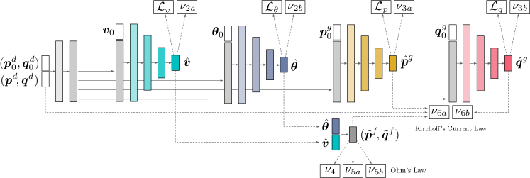
Figure 1: The OPF-DNN Model: Each layer is fully connected with ReLU activation. White boxes correspond to input tensors, dark, colored, boxes correspond to output layers. Loss components and violation degrees are shown as white rectangles.

To define the violation degrees of the AC-OPF constraints, the baseline model needs to extended to predict the reactive power dispatched $\bm{q}^{g}$ and the voltage angles $\bm{\theta}$ of the power network. Given the predicted values $\hat{\bm{v}},\hat{\bm{\theta}},\hat{\bm{p}}^{g},$ and $\hat{\bm{q}}^{g}$, the satisfiability degree of the OPF constraints can be expressed as: This section extends the homonym section of the main paper by reporting the complete set of satisfiability and violation degrees of the OPF constraints.

Given the predicted values $\hat{\bm{v}},\hat{\bm{\theta}},\hat{\bm{p}}^{g},$ and $\hat{\bm{q}}^{g}$, the satisfiability degree of the OPF constraints are expressed as follows:

$$\sigma_{2a}^{L}(\hat{v}_{i}) =(\dot{v}^{\min}_{i}-\hat{v}_{i}) \!\!\!\!\!\!\forall i\in{\cal N}$$

$$\sigma_{2a}^{R}(\hat{v}_{i}) =(\hat{v}_{i}-\dot{v}^{\max}_{i}) \!\!\!\!\!\!\forall i\in{\cal N}$$

$$\sigma_{2b}^{L}(\hat{\theta}_{ij}) =((\hat{\theta}_{j}-\hat{\theta}_{i})-\dot{\theta}^{\Delta}_{ij}) \!\!\!\!\!\!\forall(ij)\in{\cal E}$$

$$\sigma_{2b}^{R}(\hat{\theta}_{ij}) =((\hat{\theta}_{i}-\hat{\theta}_{j})-\dot{\theta}^{\Delta}_{ij}) \!\!\!\!\!\!\forall(ij)\in{\cal E}$$

$$\sigma_{3a}^{L}(\hat{p_{i}}^{g}) =\dot{p}^{g\min}_{i}-\hat{p}{}^{g}_{i} \!\!\!\!\!\!\forall i\in{\cal N}$$

$$\sigma_{3a}^{R}(\hat{p_{i}}^{g}) =\hat{p}^{g}_{i}-\dot{p}^{\max}_{i} \!\!\!\!\!\!\forall i\in{\cal N}$$

$$\sigma_{3b}^{L}(\hat{q_{i}}^{g}) =\dot{q}^{g\min}_{i}-\hat{q}{}^{g}_{i} \!\!\!\!\!\!\forall i\in{\cal N}$$

$$\sigma_{3b}^{R}(\hat{q_{i}}^{g}) =\hat{q}^{g}_{i}-\dot{q}^{\max}_{i} \!\!\!\!\!\!\forall i\in{\cal N}$$

$$\sigma_{4}(\tilde{p}^{f}_{ij},\tilde{q}^{f}_{ij}) =(\tilde{p}^{f}_{ij})^{2}+(\tilde{q}^{f}_{ij})^{2}-\dot{S}^{\max}_{ij} \!\!\!\!\!\!\forall(ij)\in{\cal E}$$

$$\sigma_{5a}(\tilde{{p}}^{f}_{ij},{p}^{f}_{ij}) =\tilde{p}^{f}_{ij}-p_{ij}^{f} \!\!\!\!\!\!\forall(ij)\in{\cal E}$$

$$\sigma_{5b}(\tilde{{q}}^{f}_{ij},{q}^{f}_{ij}) =\tilde{q}^{f}_{ij}-q^{f}_{ij} \!\!\!\!\!\!\forall(ij)\in{\cal E}$$

$$\sigma_{6a}(\hat{p}^{g}_{i},\dot{p}^{d}_{i},\tilde{\bm{p}}^{f}) =\sum_{(ij)\in{\cal E}}\tilde{p}^{f}_{ij}-(\hat{p}^{g}_{i}\!-\!\dot{p}^{d}_{i}) \!\!\!\!\!\!\forall i\in{\cal N}$$

$$\sigma_{6b}(\hat{q}^{g}_{i},\dot{q}^{d}_{i},\tilde{\bm{q}}^{f}) =\sum_{(ij)\in{\cal E}}\tilde{q}^{f}_{ij}-(\hat{q}^{g}_{i}\!-\!\dot{q}^{d}_{i}) \!\!\!\!\!\!\forall i\in{\cal N}$$

where $\sigma_{2a}^{L}$ and $\sigma_{2a}^{R}$ correspond to Constraints (2a) and capture the distance of the predictions $\hat{v}_{i}$ from exceeding the voltage bounds. The functions $\sigma_{2b}^{L}$ and $\sigma_{2b}^{R}$ correspond to Constraints ($\bar{2b}$) and express how much the difference between two voltage angles exceeds the bound. Similarly, $\sigma_{3a}^{L}$, $\sigma_{3a}^{R}$, and $\sigma_{3b}^{L}$, $\sigma_{3b}^{R}$, relate to Constraints ($\bar{3a}$) and (3b), respectively, and describe the distance of the predicted generator active and reactive dispatch from their bounds. Function $\sigma_{4}$ corresponds to Constraints ($\bar{4}$) and captures the distance of the power flow on line $(ij)$ from its bound. Therein, $\tilde{p}^{f}_{ij}$ and $\tilde{q}^{f}_{ij}$ are, respectively, the active and reactive power flow for line $(ij)\in{\cal E}$. Notice that $\tilde{p}^{f}_{ij}$ and $\tilde{q}^{f}_{ij}$ are not predicted directly, as an output of the DNN. Instead, they are computed using the predicted quantities $\hat{v}_{i},\hat{v}_{j},\hat{\theta}_{i}$, and $\hat{\theta}_{j}$ according to Constraints ($\bar{5a}$) and (5b). The quantities ${p}^{f}_{ij}$ and ${q}^{f}_{ij}$ correspond to the ground truths values. Functions $\sigma_{5a}$ and $\sigma_{5b}$ measure the deviation of the predicted flow (based on the other predicted quantities) to the ground truth values according to the Ohm’s Law (Constraints (5a) and (5b)). Finally, the functions $\sigma_{6a}$ and $\sigma_{6b}$ relate to the Kirchhoff Current Law (Constraints ($\bar{6a}$) and (6b)) and express the violation of flow conservation at a bus.

The violation degrees associated to the satisfiability degree above are defined as follows:

$$\nu_{2a}(\hat{\bm{v}}) =\frac{1}{n}\sum_{i\in{\cal N}}\left(\nu_{c}^{\geq}\big{(}\sigma_{2a}^{L}(\hat{v}_{i})\big{)}+\nu_{c}^{\geq}\big{(}\sigma_{2a}^{R}(\hat{v}_{i})\big{)}\right)$$

$$\nu_{2b}(\hat{\bm{\theta}}) =\frac{1}{e}\sum_{(ij)\in{\cal E}}\left(\nu_{c}^{\geq}\big{(}\sigma_{2b}^{L}(\hat{\theta}_{ij})\big{)}+\nu_{c}^{\geq}\big{(}\sigma_{2b}^{R}(\hat{\theta}_{ij})\big{)}\right)$$

$$\nu_{3a}(\hat{\bm{p}}) =\frac{1}{n}\sum_{i\in{\cal N}}\left(\nu_{c}^{\geq}\big{(}\sigma_{3a}^{L}(\hat{p}_{i})\big{)}+\nu_{c}^{\geq}\big{(}\sigma_{3a}^{R}(\hat{p}_{i})\big{)}\right)$$

$$\nu_{3b}(\hat{\bm{q}}) =\frac{1}{n}\sum_{i\in{\cal N}}\left(\nu_{c}^{\geq}\big{(}\sigma_{3b}^{L}(\hat{q}_{i})\big{)}+\nu_{c}^{\geq}\big{(}\sigma_{3b}^{R}(\hat{q}_{i})\big{)}\right)$$

$$\nu_{4}(\tilde{\bm{p}}^{f}\!,\tilde{\bm{q}}^{f}) =\frac{1}{e}\sum_{(ij)\in{\cal E}}\nu_{c}^{\geq}\big{(}\sigma_{4}(\tilde{p}_{ij}^{f},\tilde{q}_{ij}^{f})\big{)}$$

$$\nu_{5a}(\tilde{\bm{p}}^{f}\!,\bm{p}^{f}) =\frac{1}{e}\sum_{(ij)\in{\cal E}}\nu_{c}^{=}\big{(}\sigma_{5a}(\tilde{p}_{ij}^{f},{p}_{ij}^{f})\big{)}$$

$$\nu_{5b}(\tilde{\bm{q}}^{f}\!,\bm{q}^{f}) =\frac{1}{e}\sum_{(ij)\in{\cal E}}\nu_{c}^{=}\big{(}\sigma_{5a}(\tilde{q}_{ij}^{f},{q}_{ij}^{f})\big{)}$$

$$\nu_{6a}(\hat{\bm{p}}^{g}\!,\dot{\bm{p}}^{d}\!,\bm{p}^{f}) =\frac{1}{e}\sum_{(ij)\in{\cal E}}\nu_{c}^{=}\big{(}\sigma_{6a}(\hat{p}^{g}_{i},\dot{p}^{d}_{i},\tilde{\bm{p}}^{f})\big{)}$$

$$\nu_{6b}(\hat{\bm{q}}^{g}\!,\dot{\bm{q}}^{d}\!,\bm{q}^{f}) =\frac{1}{e}\sum_{(ij)\in{\cal E}}\nu_{c}^{=}\big{(}\sigma_{6b}(\hat{q}^{g}_{i},\dot{q}^{d}_{i},\tilde{\bm{q}}^{f})\big{)}.$$

where $n$ and $e$ denote the number of buses and transmission lines, respectively. These functions capture the average deviation by which the prediction violates the associated constraint. The violations degrees define penalties that will be used to enrich the DNN loss function to encourage their satisfaction. Prior describing the DNN objective, we introduce a further extension that exploits yet another aspect of the structure of the OPF.

Exploiting Existing Solutions

The solving of an OPF (or a load flow) rarely happens in a cold-start: OPFs are typically solved in the context of an existing operating point and/or with the availability of solutions to similar instances (hot-start). As a result, the learning task can exploit this existing configuration, which is called the hot-start state in this paper. The hot-start state is a tuple $\bm{s}_{0}={\bm{\left(}{\bm{p}^{d}_{0},\bm{q}^{d}_{0},\bm{p}^{g}_{0},\bm{q}^{g}_{0},\bm{v}_{0},\bm{\theta}_{0}}\bm{}}$, describing the load, the generation, and the voltages that are solutions to a related OPF. The learning can then use a new, enriched, training dataset, defined as follows:

$${\cal D}\!=\!\Big{\{}\!\! \big{(}(\overbrace{\bm{p}_{0}^{d},\bm{q}_{0}^{d},\bm{p}^{g}_{0},\bm{q}^{g}_{0},\bm{v}_{0},\bm{\theta}_{0},\bm{p}^{d},\bm{q}^{d}}^{\bm{x}_{1}})_{1},\overbrace{(\bm{p}^{g},\bm{q}^{g},\bm{v},\bm{\theta}}^{\bm{y}_{1}})_{1}\big{)},\ldots,$$

$$\big{(}(\underbrace{\bm{p}_{0}^{d},\bm{q}_{0}^{d},\bm{p}^{g}_{0},\bm{q}^{g}_{0},\bm{v}_{0},\bm{\theta}_{0},\bm{p}^{d},\bm{q}^{d}}_{\bm{x}_{N}})_{N},\underbrace{(\bm{p}^{g},\bm{q}^{g},\bm{v},\bm{\theta}}_{\bm{y}_{N}})_{N}\big{)}\Big{\}}.$$

The elements $\bm{x}_{\ell}\!\in\!\mathbb{R}^{8n}$ are vectors describing the hot-start state $\bm{s}_{0}$ (e.g., the configuration in the previous timestep) and the current loads $(\bm{p}^{d},\bm{q}^{d})$. The elements $\bm{y}_{\ell}\!\in\!\mathbb{R}^{4n}$ are vectors describing the optimal generator and voltage settings for input data $\bm{x}_{\ell}$. The collection of the elements $\{\bm{x}_{\ell}\}_{\ell=1}^{N}$ is denoted by ${\cal X}$ and the elements $\{\bm{y}_{\ell}\}_{\ell=1}^{N}$ by ${\cal Y}$. The goal remain that of learning a mapping $\hat{\cal O}$. Note that, despite some proximity of loads in subsequent states, the OPF non linearities often cause severe variations in the operational parameters outputs. Therefore, as confirmed by our experimental results, the learning mechanism cannot rely exclusively on the information encoded in the hot-start state.

Objective

It is now possible to define the final loss function used to train the OPF-DNN. First, the loss is augmented to consider the predictions of voltage phase angles and the reactive power of generators, since these are required to compute the violation degrees associated with the OPF constraints. The resulting loss function ${\cal L}_{o}(\bm{y},\hat{\bm{y}})$ is:

$$\underbrace{\|\bm{v}-\hat{\bm{v}}\|}_{{\cal L}_{v}(\bm{y},\hat{\bm{y}})}{\!}^{2}+\underbrace{\|\bm{\theta}-\hat{\bm{\theta}}\|}_{{\cal L}_{\theta}(\bm{y},\hat{\bm{y}})}{\!}^{2}+\underbrace{\|\bm{p}^{g}-\hat{\bm{p}}^{g}\|}_{{\cal L}_{p}(\bm{y},\hat{\bm{y}})}{\!}^{2}+\underbrace{\|\bm{q}^{g}-\hat{\bm{q}}^{g}\|}_{{\cal L}_{q}(\bm{y},\hat{\bm{y}})}{\!}^{2}.$$ (9)

It minimizes the mean squared error between the optimal voltage and generator settings $\bm{y}$ and the predicted ones $\hat{\bm{y}}$.

Moreover, the objective function includes the Lagrangian relaxation based on the OPF physical and engineering constraints violation degrees. Given the set ${\cal C}$ of OPF constraints, the associated loss is captured by the expression

$${\cal L}_{c}(\bm{x},\hat{\bm{y}}) =\sum_{c\in{\cal C}}\lambda_{c}\nu_{c}(\bm{x},\hat{\bm{y}}).$$

The model loss function sums these two terms, i.e.,

$${\cal L}(\bm{x},\bm{y},\hat{\bm{y}})={\cal L}_{o}(\bm{y},\hat{\bm{y}})+{\cal L}_{c}(\bm{x},\hat{\bm{y}}).$$

The Network Architecture

The network architecture is outlined in Figure 1. The input layers on the left process the tensor of loads $(\bm{p}^{d}_{0},\bm{q}^{d}_{0})$ of the hot-start state $\bm{s}_{0}$ and the input loads $(\bm{p}^{d},\bm{q}^{d})$. The network has 4 basic units, each following a decoder-encoder structure and composed by a number of fully connected layers with ReLU activations. Each subnetwork predicts a target variable: voltage magnitudes $\hat{\bm{v}}$, phase angles $\hat{\bm{\theta}}$, active power generations $\hat{\bm{p}}^{g}$, and reactive power generations $\hat{\bm{q}}^{g}$. Each sub-network takes as input the corresponding tensor in the hot-start state $\bm{s}_{0}$ (e.g., the sub-network responsible for predicting the voltage magnitude $\hat{\bm{v}}$ takes as input $\bm{v}_{0}$), as well as the last hidden layer of its input subnetwork, that processes the load tensors.

The predictions for the voltage magnitude $\hat{\bm{v}}$ and angle $\hat{\bm{\theta}}$ are used to compute the load flows $(\tilde{\bm{p}}^{f},\tilde{\bm{q}}^{f}\!)$, as illustrated on the bottom of the Figure. The components of the losses are highlighted in the white boxes and a full description of the network architecture is provided in the Appendix.

Lagrangian Duality

Let $\hat{\cal O}[\bm{w}]$ be the resulting OPF-DNN with weights $\bm{w}$ and let ${\cal L}[\bm{\lambda}]$ be the loss function parametrized by the Lagrangian multipliers $\bm{\lambda}=\{\lambda_{c}\}_{c\in{\cal C}}$. The training aims at finding the weights $\bm{w}$ that minimize the loss function for a given set of Lagrangian multipliers, i.e., it computes

$${\it LR}(\bm{\lambda})=\min_{\bm{w}}{\cal L}[\bm{\lambda}](\bm{x},\bm{y},\hat{\cal O}[\bm{w}](\bm{x})).$$

It remains to determine appropriate Lagrangian multipliers. This paper proposes the use of Lagrangian duality to obtain the optimal Lagrangian multipliers when training the OPF-DNN, i.e., it solves

$${\it LD}=\max_{\bm{\lambda}}{\it LR}(\bm{\lambda}).$$

The Lagrangian dual is solved through a subgradient method that computes a sequence of multipliers $\bm{\lambda}^{1},\ldots,\bm{\lambda}^{k},\ldots$ by solving a sequence of trainings ${\it LR}(\bm{\lambda}^{0}),\ldots,{\it LR}(\bm{\lambda}^{k-1}),\ldots$ and adjusting the multipliers using the violations, i.e.,

$$\bm{w}^{k+1} =\operatorname*{argmin}_{\bm{w}}{\cal L}[\bm{\lambda}^{k}](\bm{x},\bm{y},\hat{\cal O}[\bm{w}^{k}](\bm{x}))$$ (L1)

$$\bm{\lambda}^{k+1} ={\bm{\left(}{\lambda^{k}_{c}+\rho\,\nu_{c}(\bm{x},\hat{\cal O}[\bm{w}^{k+1}](\bm{x}))\;|\;c\in{\cal C}}\bm{}}.$$ (L2)

In the implementation, step (L1) is approximated using a Stochastic Gradient Descent (SGD) method. Importantly, this step does not recomputes the training from scratch but uses a hot start for the weights $\bm{w}$.

The overall training scheme is presented in Algorithm 1. It takes as input the training dataset $({\cal X},{\cal Y})$, the optimizer step size $\alpha>0$ and the Lagrangian step size $\rho>0$. The Lagrangian multipliers are initialized in line 1. The training is performed for a fixed number of epochs, and each epoch optimizes the weights using a minibatch of size $b$. After predicting the voltage and generation power quantities (line 1), the objective and constraint losses are computed (lines 1 and 1). The latter uses the Lagrangian multipliers $\bm{\lambda}^{k}$ associated with current epoch $k$. The model weights are updated in line 1. Finally, after each epoch, the Lagrangian multipliers are updated following step (L2) described above (lines 1 and 1).

1

input : $({\cal X},{\cal Y}):$ Training data

$\alpha,\rho:$ Optimizer and Lagrangian step sizes, reps.​​​​​​​​​​

2 $\bm{\lambda}^{0}\leftarrow 0\;\;\forall c\in{\cal C}$

3 for epoch $k=0,1,\ldots$ do

4       foreach $(\bm{x},\bm{y})\!\leftarrow\!\mbox{minibatch}({\cal X},{\cal Y})$ of size $b$ do

5             $\hat{\bm{y}}\leftarrow\hat{\cal O}[\bm{w}](\bm{x})$

6             ${\cal L}_{o}(\hat{\bm{y}},\bm{y})\leftarrow\frac{1}{b}\sum_{\ell\in[b]}{\cal L}_{v}(\bm{y}_{\ell},\hat{\bm{y}}_{\ell})+{\cal L}_{\theta}(\bm{y}_{\ell},\hat{\bm{y}}_{\ell})+$​​​​

             $\hskip 87.0pt{\cal L}_{p}(\bm{y}_{\ell},\hat{\bm{y}}_{\ell})+{\cal L}_{q}(\bm{y}_{\ell},\hat{\bm{y}}_{\ell})$

7             ${\cal L}_{c}(\bm{x},\hat{\bm{y}})\leftarrow\frac{1}{b}\sum_{\ell\in[b]}\sum_{c\in{\cal C}}\lambda_{c}^{k}\nu_{c}(\bm{x}_{\ell},\hat{\bm{y}}_{\ell})$

8             $\omega\leftarrow\omega-\alpha\nabla_{\omega}({\cal L}_{o}(\hat{\bm{y}},\bm{y})+{\cal L}_{c}(\bm{x},\hat{\bm{y}}))\!\!\!\!$

9      foreach $c\in{\cal C}$ do

10             $\lambda^{k+1}_{c}\leftarrow\lambda^{k}+\rho\nu_{c}(\bm{x},\hat{\bm{y}})$

11      

Algorithm 1 Learning Step

						$\Delta_{1\%}~{}p^{d}$		$\Delta_{2\%}~{}p^{d}$		$\Delta_{3\%}~{}p^{d}$
Test Case	$|{\cal N}|$	$|{\cal E}|$	$l$	$g$	$|({\cal X},{\cal Y})|$	$(\%)$	MW	$(\%)$	MW	$(\%)$	MW
14_ieee	14	40	11	2	395806	2.05	5.3	2.59	6.7	3.15	8.2
30_ieee	30	82	21	2	273506	2.47	7.0	2.94	8.3	3.36	9.5
39_epri	39	92	21	10	287390	2.49	156.3	2.94	183.9	3.42	213.9
57_ieee	57	160	42	4	269140	2.65	33.2	3.19	39.9	3.67	45.9
73_ieee_rts	73	240	51	73	373142	2.72	233.2	3.28	281.2	3.80	324.9
89_pegase	89	420	35	12	338132	2.50	204.0	3.06	250.1	3.53	288.0
118_ieee	118	372	99	19	395806	3.03	128.6	3.50	148.8	3.98	169.1
162_ieee_dtc	162	568	113	12	237812	3.10	296.5	3.54	337.9	4.04	385.9
189_edin	189	412	41	35	69342	2.85	39.1	3.27	44.8	3.72	50.9
300_ieee	300	822	201	57	235732	3.25	775.9	3.78	902.8	4.22	1007.0

Table 1: The Power Networks Adopted as Benchmarks.

Experiments

This section evaluates the predictive accuracy of OPF-DNN and compares it to the AC model and its linear DC approximation. It also analyzes various design decisions in detail.

Data sets

The experiments examine the proposed models on a variety of mid-sized power networks from the NESTA library (?). The ground truth data are constructed as follows: For each network, different benchmarks are generated by altering the amount of nominal load $\bm{x}\!=\!(\bm{p}^{d},\bm{q}^{d})$ within a range of $\pm 20\%$. The loads are thus sampled from the distributions $\bm{x}^{\prime}=(\bm{p}^{d}{}^{\prime},\bm{q}^{d}{}^{\prime})\sim\text{Uniform}(0.8\bm{x},1.2\bm{x})$. Notice that the resulting benchmarks have load demands that vary by a factor of up to $20\%$ of their nominal values: Many of them become congested and significantly harder computationally than their original counterparts. A network value that constitutes a dataset entry $(\bm{x}^{\prime},\bm{y}^{\prime})$ is a feasible OPF solution obtained by solving the AC-OPF problem detailed in Model 1.

When the learning step exploits an existing hot-start state $\bm{s}_{0}$, the training test cases have the property that the total active loads $\|\bm{p}^{d}_{0}\|_{1}$ in $\bm{s}_{0}$ are within 1, 2, and 3% of the total active loads $\|\bm{p}^{d}\|_{1}$. Note that, while the aggregated loads follow this restriction, the individual loads may have greater variations. Those are illustrated in Table 1 for the 1% ($\Delta_{1\%}p^{d}$), 2% ($\Delta_{2\%}p^{d}$) and 3% ($\Delta_{3\%}p^{d}$) cases, where the average variations are expressed both in percentage of the total load and in absolute values (MWs). As can be seen, the variations are significant. The table also describes the dataset sizes, including the number of buses $|{\cal N}|$ and transmission lines $|{\cal E}|$ of the networks. The column titled $l$ and $g$ denote, respectively, the number of load and generator buses of the networks. The data are normalized using the per unit (pu) system so that all quantities are close to 1. The experiments use a $80/20$ train-test split and report results on the test set.

Settings

The experiments examine the OPF-DNN models whose features are summarized in Table 2. ${\cal M}_{\text{B}}$ refers to the baseline model: It minimizes the loss function ${\cal L}_{o}$ described in Equation (8). ${\cal M}_{\text{C}}$ exploits the problem constraints and minimizes the loss: ${\cal L}_{o}+\sum_{c\in{\cal C}}\lambda_{c}\nu_{c}$, with ${\cal L}_{o}$ defined in Equation (9) and all $\lambda_{c}$ set to $1$. The suffix $S$ is used for the models that exploit a hot-start state, and $D$ is used for the model that exploit the Lagrangian dual scheme. In particular, ${\cal M}_{\text{C}}^{\text{D}}$ extends ${\cal M}_{\text{C}}$ by learning the Lagrangian multipliers $\lambda_{c}$ using the Lagrangian dual scheme described in Algorithm 1. ${\cal M}_{\text{CS}}$ uses the same loss function as ${\cal M}_{\text{C}}$, but it adopts the architecture outlined in Figure 1. ${\cal M}_{\text{CS}}^{\text{L}}$ sets the Lagrangian weights as trainable parameters and learns them during the training cycle. Finally, ${\cal M}_{\text{CS}}^{\text{D}}$ extends ${\cal M}_{\text{CS}}$ by learning the Lagrangian multipliers $\lambda_{c}$ using the Lagrangian dual scheme (see Algorithm 1). The latter model is also denoted with OPF-DNN in the paper. The details of the models architectures and loss functions are provided in the appendix. All the models that exploit a hot-start state are trained over datasets using states differing by at most $1\%$. The section also reports a comparison of the DNN-OPF model trained over hot-start state datasets using states differing by at most $1$, $2$, and $3\%$.

Model	${\cal M}_{\text{B}}$	${\cal M}_{\text{C}}$	${\cal M}_{\text{C}}^{\text{D}}$	${\cal M}_{\text{CS}}$	${\cal M}_{\text{CS}}^{\text{L}}$	${\cal M}_{\text{CS}}^{\text{D}}$
Exploit Constraints	$\Box$	$\text{\hbox to0.0pt{$\checkmark$\hss}}\Box$	$\text{\hbox to0.0pt{$\checkmark$\hss}}\Box$	$\text{\hbox to0.0pt{$\checkmark$\hss}}\Box$	$\text{\hbox to0.0pt{$\checkmark$\hss}}\Box$	$\text{\hbox to0.0pt{$\checkmark$\hss}}\Box$
Exploit hot-start State	$\Box$	$\Box$	$\Box$	$\text{\hbox to0.0pt{$\checkmark$\hss}}\Box$	$\text{\hbox to0.0pt{$\checkmark$\hss}}\Box$	$\text{\hbox to0.0pt{$\checkmark$\hss}}\Box$
Train Lagrangian weights	$\Box$	$\Box$	$\Box$	$\Box$	$\text{\hbox to0.0pt{$\checkmark$\hss}}\Box$	$\Box$
Lagrangian Dual update	$\Box$	$\Box$	$\text{\hbox to0.0pt{$\checkmark$\hss}}\Box$	$\Box$	$\Box$	$\text{\hbox to0.0pt{$\checkmark$\hss}}\Box$

Table 2: The DNN Models Adopted.

The models were implemented using the Julia package PowerModels.jl (?) with the nonlinear solver IPOPT (?) for solving the nonlinear AC model and its the DC approximation. The DDN models were implemented using PyTorch (?) with Python 3.0. The training was performed using NVidia Tesla V100 GPUs and and 2GHz Intel Cores. The AC and DC-OPF models were solved using the same CPU cores. Training each network requires less than 2GB of RAM. The training uses the Adam optimizer with learning rate ($\alpha\!=\!0.001$) and $\beta$ values $(0.9,0.999)$ and was performed for $80$ epochs using batch sizes $b=64$. Finally, the Lagrangian step size $\rho$ is set to $0.01$.

Prediction Errors

Test case	Model	$\hat{\bm{p}}^{g}$	$\hat{\bm{q}}^{g}$	$\hat{\bm{v}}$	$\hat{\bm{\theta}}$	$\tilde{\bm{p}}^{f}$	Test case	Model	$\hat{\bm{p}}^{g}$	$\hat{\bm{q}}^{g}$	$\hat{\bm{v}}$	$\hat{\bm{\theta}}$	$\tilde{\bm{p}}^{f}$
14_ieee	${\cal M}_{\text{B}}$	5.7820	11.004	0.7310	1.4050	1.9070	89_pegase	${\cal M}_{\text{B}}$	0.2516	0.2250	90.689	37.176	3133.4
	${\cal M}_{\text{C}}$	6.1396	11.315	1.2790	1.4100	0.4640		${\cal M}_{\text{C}}$	0.3589	0.2320	77.295	7.9760	42.962
	${\cal M}_{\text{C}}^{\text{D}}$	5.5698	7.1120	6.0682	0.0500	0.4970		${\cal M}_{\text{C}}^{\text{D}}$	0.3549	0.3361	2.8380	17.921	24.529
	${\cal M}_{\text{CS}}$	0.2756	0.6980	0.1180	0.1480	0.1050		${\cal M}_{\text{CS}}$	0.1074	0.0860	9.4168	0.8240	6.4130
	${\cal M}_{\text{CS}}^{\text{L}}$	0.2703	0.7450	0.1860	0.0760	0.1690		${\cal M}_{\text{CS}}^{\text{L}}$	0.1014	0.0830	10.199	0.9120	9.3560
	${\cal M}_{\text{CS}}^{\text{D}}$	0.0234	0.0470	0.0050	0.0070	0.0530		${\cal M}_{\text{CS}}^{\text{D}}$	0.0797	0.0770	0.0862	0.0530	5.0160
30_ieee	${\cal M}_{\text{B}}$	3.3465	2.0270	14.699	4.3400	27.213	118_ieee	${\cal M}_{\text{B}}$	0.2150	2.9910	7.1520	4.2600	38.863
	${\cal M}_{\text{C}}$	3.1289	1.3380	2.7346	1.5930	1.6820		${\cal M}_{\text{C}}$	0.1810	3.2570	6.9150	4.6520	6.4730
	${\cal M}_{\text{C}}^{\text{D}}$	3.1230	1.1096	0.1596	0.2590	2.3000		${\cal M}_{\text{C}}^{\text{D}}$	0.1787	1.0840	10.002	0.2160	2.8100
	${\cal M}_{\text{CS}}$	0.3052	0.1104	0.3130	0.0580	0.2030		${\cal M}_{\text{CS}}$	0.0380	0.6900	0.1170	1.2750	0.6640
	${\cal M}_{\text{CS}}^{\text{L}}$	0.2900	0.3200	0.3120	0.0600	0.1600		${\cal M}_{\text{CS}}^{\text{L}}$	0.0380	0.6870	0.1380	1.2750	0.6100
	${\cal M}_{\text{CS}}^{\text{D}}$	0.0055	0.0320	0.0070	0.0041	0.0620		${\cal M}_{\text{CS}}^{\text{D}}$	0.0340	0.6180	0.0290	0.2070	0.4550
39_epri	${\cal M}_{\text{B}}$	0.2299	1.2600	98.726	58.135	202.67	162_ieee	${\cal M}_{\text{B}}$	0.2310	1.2070	9.1810	5.4800	82.076
	${\cal M}_{\text{C}}$	0.2180	1.2790	17.104	2.5940	80.064		${\cal M}_{\text{C}}$	0.2820	1.6120	7.1210	5.3620	14.706
	${\cal M}_{\text{C}}^{\text{D}}$	0.2216	1.2610	2.7346	4.0730	41.395		${\cal M}_{\text{C}}^{\text{D}}$	0.2772	0.9873	6.8359	1.1950	15.456
	${\cal M}_{\text{CS}}$	0.0559	0.1080	2.2350	0.2880	1.8360		${\cal M}_{\text{CS}}$	0.0750	0.3760	0.1760	0.3720	0.7520
	${\cal M}_{\text{CS}}^{\text{L}}$	0.0533	0.1440	2.2010	0.2040	2.2000		${\cal M}_{\text{CS}}^{\text{L}}$	0.0750	0.3690	0.1750	0.3950	0.6750
	${\cal M}_{\text{CS}}^{\text{D}}$	0.0024	0.0720	0.0280	0.0100	1.2660		${\cal M}_{\text{CS}}^{\text{D}}$	0.0710	0.2440	0.0770	0.3660	0.4920
57_ieee	${\cal M}_{\text{B}}$	2.3255	1.6380	5.1002	1.5680	14.386	189_edin	${\cal M}_{\text{B}}$	0.4979	0.1160	42.295	5.2970	4371.1
	${\cal M}_{\text{C}}$	2.2658	1.4850	3.5402	2.0890	2.8850		${\cal M}_{\text{C}}$	0.5748	0.0890	18.577	3.9640	24.918
	${\cal M}_{\text{C}}^{\text{D}}$	2.2708	1.5138	9.5861	0.0680	1.6170		${\cal M}_{\text{C}}^{\text{D}}$	0.4081	0.0711	7.3091	3.2220	15.774
	${\cal M}_{\text{CS}}$	0.1308	0.3320	0.2150	0.0430	0.2410		${\cal M}_{\text{CS}}$	0.1178	0.0190	1.9913	0.7040	3.8470
	${\cal M}_{\text{CS}}^{\text{L}}$	0.1340	0.3300	0.2110	0.0360	0.2280		${\cal M}_{\text{CS}}^{\text{L}}$	0.1178	0.0180	2.4300	0.4960	3.5810
	${\cal M}_{\text{CS}}^{\text{D}}$	0.0170	0.0231	0.0150	0.0080	0.1520		${\cal M}_{\text{CS}}^{\text{D}}$	0.0907	0.0110	0.0982	0.3330	1.6520
73_ieee	${\cal M}_{\text{B}}$	0.2184	0.0380	18.414	5.0550	106.08	300_ieee	${\cal M}_{\text{B}}$	0.0838	0.0900	28.025	12.137	125.47
	${\cal M}_{\text{C}}$	0.0783	0.0360	2.8074	1.2500	7.8630		${\cal M}_{\text{C}}$	0.0914	0.0860	14.727	7.7450	34.133
	${\cal M}_{\text{C}}^{\text{D}}$	0.0775	0.5302	2.7038	0.3880	6.2980		${\cal M}_{\text{C}}^{\text{D}}$	0.0529	0.0491	11.096	7.3830	27.554
	${\cal M}_{\text{CS}}$	0.0061	0.0160	0.2192	0.1190	0.4890		${\cal M}_{\text{CS}}$	0.0174	0.0240	3.1130	7.2330	26.905
	${\cal M}_{\text{CS}}^{\text{L}}$	0.0063	0.0150	0.3156	0.1260	0.4160		${\cal M}_{\text{CS}}^{\text{L}}$	0.0139	0.0240	0.2180	4.6480	2.0180
	${\cal M}_{\text{CS}}^{\text{D}}$	0.0050	0.0101	0.0235	0.1180	0.3300		${\cal M}_{\text{CS}}^{\text{D}}$	0.0126	0.0190	0.0610	2.5670	1.1360

Table 3: Prediction Errors (%).

This section first analyzes the prediction error of the DNN models. Table 3 reports the average L1 distance between the predicted generator active $\hat{\bm{p}}^{g}$ and reactive $\hat{\bm{q}}^{g}$ power, voltage magnitude $\hat{\bm{v}}$ and angles $\hat{\bm{\theta}}$ and the original quantities. It also reports the errors of the predicted flows $\tilde{\bm{p}}^{f}$ (which use the generator power and voltage predictions) and are important to assess the fidelity of the predictions. The distances are reported in percentage: $\frac{\|\hat{\bm{x}}-\bm{x}\|_{1}}{\|\bm{x}\|_{1}}\!\times\!100$, for quantity $\bm{x}$, and best results are highlighted in bold. For completeness, the results report an extended version of model ${\cal M}_{\text{B}}$, that allow us to predict quantities $\bm{\theta}$ and $\bm{q}^{d}$. The latter were obtained by extending ${\cal M}_{\text{B}}$ network using two additional layers, Out-$\bm{\theta}$ and Out-$\bm{q}^{g}$ for, respectively, predicting the voltage angles and the reactive generator power, analogously to those in model ${\cal M}_{\text{C}}$. Additionally, its loss function was extended as:

$${\cal L}_{o}(\bm{y},\hat{\bm{y}}) =\|\bm{v}-\hat{\bm{v}}\|^{2}+\|\bm{\theta}-\hat{\bm{\theta}}\|^{2}$$

$$+\|\bm{p}^{g}-\hat{\bm{p}}^{g}\|^{2}+\|\bm{q}^{g}-\hat{\bm{q}}^{g}\|^{2}.$$

The prediction errors for quantities $\bm{p}^{g}$ and $\bm{v}$ did not degrade in this extended version with respect to those predicted by the simple ${\cal M}_{\text{B}}$ network.

A clear trend appears: The prediction errors decrease with the increasing of the model complexity. In particular, model ${\cal M}_{\text{C}}$, which exploits the problem constraints, predicts much better voltage quantities and power flows than ${\cal M}_{\text{B}}$. The use of the Lagrangian Duals, in model $\cal{M}_{\text{CS}}$, further improve the predictions, especially those associated to the voltage magnitude and angles and power flows. ${\cal M}_{\text{CS}}$, which exploits the problem constraints and a hot-start state, improves ${\cal M}_{\text{C}}$ predictions by one order of magnitude in most of the cases. Finally, the use of the Lagrangian dual to find the best weights (${\cal M}_{\text{CS}}^{\text{D}}$) further improves ${\cal M}_{\text{CS}}$ predictions by up to an additional order of magnitude.

Figure 2 and 3 further illustrate the importance of modeling the problem constraints and exploiting a hot-start state. The figures illustrate the prediction errors on the operational parameters $\bm{v}$ and $\bm{p}^{g}$, as well as on the angle magnitude $\bm{\theta}$ and the power flows $\bm{p}^{f}$, at the varying of the load demands in the power networks (from -20% to 20% of the aggregated nominal load values). The reason for the differences in the $x$-axis range in the various networks, is due to that, the increased load values may produce congested scenarios that cannot be accommodated. The plots are in log-10 scale and clearly indicate that the models exploiting the problem structure better generalize to the different network settings.

NESTA case 14_ieee

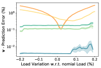
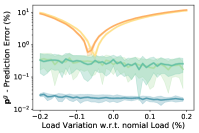
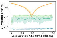
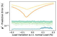
NESTA case 30_ieee

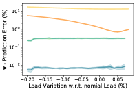
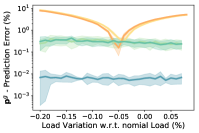
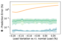
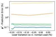
NESTA case 39_epri

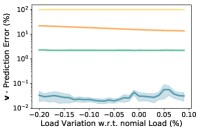
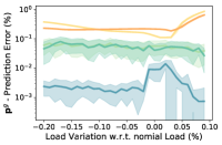
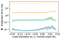
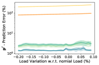
NESTA case 57_ieee

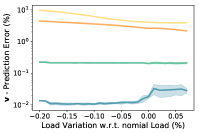
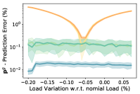
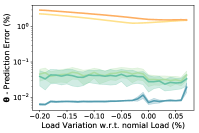
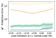
NESTA case 73_ieee_rts

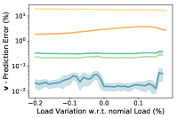
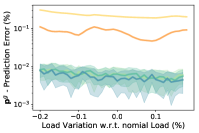
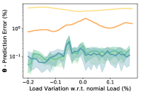
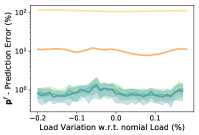
Figure 2: Prediction Errors (%) at the varying of the nominal network loads.

NESTA case 89_pegase

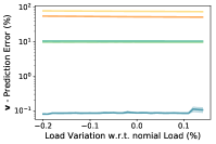
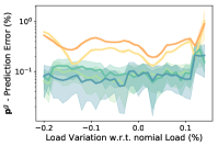
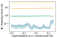
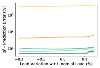
NESTA case 118_ieee

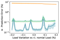
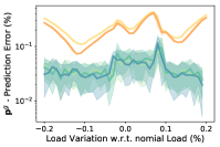
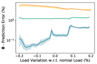
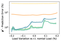
NESTA case 162_ieee_dtc

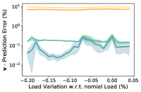
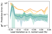
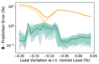
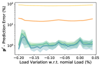
NESTA case 189_edin

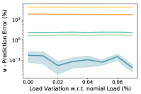
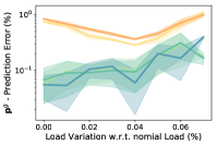
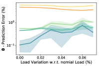
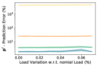
NESTA case 300_ieee

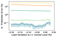
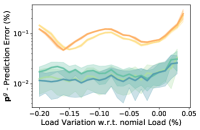
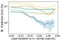
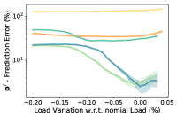
Figure 3: Prediction Errors (%) at the varying of the nominal network loads.

Test case		DC	${\cal M}_{\text{B}}$	${\cal M}_{\text{C}}$	${\cal M}_{\text{C}}^{\text{D}}$	${\cal M}_{\text{CS}}$	${\cal M}_{\text{CS}}^{\text{L}}$	${\cal M}_{\text{CS}}^{\text{D}}$	DC	${\text{LF}_{S}}$	${\cal M}_{\text{B}}$	${\cal M}_{\text{C}}$	${\cal M}_{\text{C}}^{\text{D}}$	${\cal M}_{\text{CS}}$	${\cal M}_{\text{CS}}^{\text{L}}$	${\cal M}_{\text{CS}}^{\text{D}}$
14_ieee	$\bm{p}^{g}$	2.4020	5.7048	6.0474	5.5056	0.2131	0.2052	0.0233	0.1359	4.3518	1.1061	0.8154	0.8314	0.2649	0.2571	0.0003
	$\bm{v}$	1.8352	0.9174	0.8636	0.3169	0.0937	0.0944	0.0017	3.0365	0.3450	0.3075	0.7808	0.6916	0.1516	0.2170	0.0018
30_ieee	$\bm{p}^{g}$	2.6972	2.0793	1.9688	1.7344	0.1815	0.1320	0.0007	0.1907	13.504	2.1353	1.8268	1.5523	0.2735	0.2853	0.0058
	$\bm{v}$	1.2929	83.138	0.4309	0.2869	0.0944	0.0728	0.0037	3.4931	0.4829	6.2996	2.7458	0.2270	0.4299	0.4168	0.0086
39_epri	$\bm{p}^{g}$	0.0731	0.2067	0.1700	0.0857	0.0516	0.0488	0.0005	0.2163	2.1260	0.1350	0.1467	0.1160	0.0140	0.0155	0.0023
	$\bm{v}$	1.1086	95.944	4.2008	22.921	0.3273	0.3131	0.0222	1.7251	0.8573	6.8089	3.1999	6.7880	2.3860	2.3476	0.0313
57_ieee	$\bm{p}^{g}$	0.3354	0.9733	0.7507	0.8837	0.1166	0.1165	0.0076	0.0112	4.7722	1.2882	1.2378	1.4518	0.1710	0.1752	0.0206
	$\bm{v}$	0.9091	4.0504	2.5770	0.4038	0.1771	0.1650	0.0384	0.2825	1.2243	1.5682	1.1176	0.4724	0.2772	0.2626	0.0482
73_ieee_rts	$\bm{p}^{g}$	0.0204	0.2078	0.0482	0.0214	0.0054	0.0053	0.0053	0.0304	5.2103	0.1144	0.0543	0.0239	0.0081	0.0082	0.0077
	$\bm{v}$	0.1528	14.074	0.1995	0.4470	0.0611	0.0599	0.0337	4.1537	0.1496	4.8500	2.8951	0.2525	0.2488	0.3433	0.0516
89_pegase	$\bm{p}^{g}$	0.1641	0.1440	0.2228	0.2166	0.0420	0.0443	0.0486	3.0662	7.3622	0.1834	0.2524	0.2623	0.0900	0.1035	0.0827
	$\bm{v}$	3.8584	86.795	73.506	56.519	5.6660	6.4734	1.2492	1.1776	0.6913	4.1315	4.0437	4.0373	3.9890	3.9410	1.2610
118_ieee	$\bm{p}^{g}$	0.2011	0.1071	0.0359	0.0216	0.0043	0.0056	0.0038	0.5865	3.8034	0.1353	0.1557	0.1050	0.0372	0.0391	0.0368
	$\bm{v}$	1.9971	3.4391	0.8995	0.0791	0.0956	0.0920	0.0866	2.2780	0.9772	4.5972	6.0326	0.4303	0.1599	0.1768	0.1335
162_ieee_dtc	$\bm{p}^{g}$	0.6727	0.1054	0.0673	0.1442	0.0587	0.0571	0.0558	0.6917	17.873	0.1648	0.2389	0.1575	0.0977	0.0981	0.0954
	$\bm{v}$	3.7718	3.6372	6.7930	4.2568	0.3276	0.3202	0.2565	0.5820	1.4595	0.4378	0.6922	0.5824	0.2846	0.2906	0.2921
189_edin	$\bm{p}^{g}$	1.0514	0.2694	0.3742	0.1915	0.0951	0.0966	0.0438	0.9891	3.9627	0.3669	0.5026	0.3999	0.1194	0.1202	0.0869
	$\bm{v}$	5.5054	39.188	3.5797	10.661	1.6986	2.4568	0.1041	0.4561	0.4525	1.8800	1.3474	1.6144	0.3469	0.4621	0.0882
300_ieee	$\bm{p}^{g}$	0.1336	0.0447	0.0339	0.0241	0.0091	0.0096	0.0084	0.1717	14.813	0.0644	0.0766	0.0476	0.0204	0.0205	0.0175
	$\bm{v}$	3.8526	31.698	10.292	4.0253	0.2383	2.2161	0.1994	0.6854	1.5737	2.9985	2.1296	2.3136	1.1553	0.2539	0.2196
Total Avg. (%)	$\bm{p}^{g}$	0.7751	0.9843	0.9719	0.8829	0.0777	0.0721	0.0198	0.6090	0.8214	0.5694	0.5307	0.4948	0.1096	0.1123	0.0356
	$\bm{v}$	2.4284	36.2881	10.3342	9.9916	0.8780	1.2264	0.1995	1.7870	0.9818	3.3879	2.4985	1.7409	0.9429	0.8712	0.2136

Table 4: Average distances (%) for the active power (top rows) and voltage magnitude (bottom rows) of the Load Flow solutions w.r.t. the corresponding predictions (left table) and w.r.t. the AC-OPF solutions (right table).

Load Flow Analysis

Having assessed the predictive capabilities of OPF-DNN, the next results focus on evaluating its practicality by simulating the prediction results in an operational environment. The idea is to measure how much the predictions need to be adjusted in order to satisfy the operational and physical constraints. The experiments perform a load flow (Model 2) on the predicted $\hat{\bm{p}}^{g}$ and $\hat{\bm{v}}$ values. In addition to comparing the DNN model variants, the results also report the deviations of the linear DC model from an AC-feasible solution. The DC model is widely used in power system industry. The results also reports the performance of a baseline load flow model ${\text{LF}_{S}}$ that finds a feasible solution using the hot-start state $\bm{s}_{0}$ as reference point in its objective function. These results highlight the value of learning in OPF-DNN: The reference point alone is not sufficient to find high quality solutions.

The results are tabulated in Table 4. The left table reports the L1 distances, in percentage, of the predictions $\hat{\bm{p}}^{g}$ and $\hat{\bm{v}}$ to the solutions $\bm{p}^{g}$ and $\bm{v}$ of the load flows. Trends similar to the previous section are observed, with ${\cal M}_{\text{CS}}^{\text{D}}$ being substantially more accurate than all other DNN versions. The table also shows that ${\cal M}_{\text{CS}}^{\text{D}}$ is up to two orders of magnitude more precise than the DC model. The right table reports the L1 distances of the load flow solutions to the optimal AC-OPF solutions. The results follow a similar trend, with the OPF-DNN model (${\cal M}_{\text{CS}}^{\text{D}}$) being at least one order of magnitude more precise than the DC model and the baseline ${\text{LF}_{S}}$ model. The bottom rows of the table show the average results over all the power network adopted in the experimental analysis. Note that the very high accuracy of OPF-DNN may render the use of a load flow optimization, to restore feasibility, unnecessary. These results are significant: They suggest that OPF-DNN has the potential to replace the DC model as an AC-OPF approximation and deliver generator setpoints with greater fidelity.

Test Case	DC	${\text{LF}_{S}}$	${\cal M}_{\text{B}}$	${\cal M}_{\text{C}}$	${\cal M}_{\text{CS}}$	${\cal M}_{\text{CS}}^{\text{D}}$
14_ieee	5.1792	4.5246	0.7562	0.6290	0.2614	0.0007
30_ieee	7.9894	8.2411	2.9447	2.1316	0.5433	0.0180
39_epri	0.9094	2.2869	0.1901	0.0752	0.0537	0.0003
57_ieee	1.7758	3.8445	1.1115	1.0609	0.2025	0.0527
73_ieee_rts	2.6846	1.4581	9.4364	3.2399	0.5143	0.4586
89_pegase	1.5089	2.6287	0.3284	0.3274	0.3347	0.1494
118_ieee	4.7455	1.0389	1.0973	1.1897	0.5300	0.5408
162_ieee_dtc	6.2090	4.2094	0.5021	0.8360	0.3162	0.2845
189_edin	9.9803	7.5561	5.3851	2.7770	0.7135	0.3177
300_ieee	4.7508	6.6394	1.9543	1.1576	0.3233	0.3011
Total Avg. (%)	4.5733	4.2428	2.3706	1.3424	0.3793	0.2124

Table 5: Load Flow vs. AC-OPF cost distances (%).

Solution Quality and Runtime

The next results compare the accuracy and runtime of the proposed DNN models, the DC approximation, and the load flow baseline ${\text{LF}_{S}}$, against the optimal AC-OPF solutions. The solution quality is measured by first finding the closest AC feasible solution to the predictions returned by the DC or by the DNN models. Then, the cost of the dispatches are compared to the original ones. Table 5 reports the average L1-distances of the dispatch costs. The last row reports the average distances across all the test cases. The analysis of the DNN variants exhibits the same trends as before, with the networks progressively improving the results as they exploit the problem constraints (${\cal M}_{\text{C}}$), a hot-start state (${\cal M}_{\text{CS}}$), and use the Lagrangian dual (${\cal M}_{\text{CS}}^{\text{D}}$).

Test Case	AC	${\text{LF}_{S}}$	DC	OPF-DNN
14_ieee	0.0332	0.0430	0.0075	0.0000
30_ieee	0.1023	0.0755	0.0148	0.0000
39_epri	0.2169	0.0968	0.0232	0.0000
57_ieee	0.3288	0.1394	0.0359	0.0000
73_ieee_rts	0.3081	0.2979	0.0496	0.0000
89_pegase	1.4503	0.6014	0.0601	0.0000
118_ieee	0.4207	0.7819	0.0785	0.0001
162_ieee_dtc	1.8909	0.7393	0.2016	0.0000
189_edin	4.0081	0.4490	0.0865	0.0001
300_ieee	8.0645	1.4850	0.2662	0.0001
Avg speedup	$1$x	$2.76$x	$15.2$x	$>\!10^{4}$x

Table 6: Average runtime in seconds.

Table 6 illustrates the average time required to find an AC OPF solution, the AC load flow with a reference solution, a linear DC approximation, and a prediction using OPF-DNN (${\cal M}_{\text{CS}}^{\text{D}}$) on the test dataset. Recall that the dataset adopted uses a load stress value of up to 20% of the nominal loads and hence the test cases are often much more challenging than their original counterparts. The last row of the table reports the average speedup of the models compared to the AC OPF. Observe that OPF-DNN finds dispatches whose costs are at least one order of magnitude closer to the AC solution than those returned by the DC approximation, while being several order of magnitude faster.

Hot-Start Robustness Analysis

Finally, the last results analyze the robustness of the DNN-OPF model when trained using test cases whose hot-start states differ from the input state by 1%, 2%, and 3% in the total active loads.

Table 7 reports the average L1 distances (in percentage) between the predicted generator power $\hat{\bm{p}}^{g}$, voltage magnitude $\hat{\bm{v}}$, voltage angles $\hat{\bm{\theta}}$ and the original quantities. It also reports the errors of the predicted flows $\tilde{\bm{p}}^{f}$ which use the generator power and voltage predictions. Table 8 illustrates the load flow results. The left table reports the L1 distances, in percentage, of the predictions $\hat{\bm{p}}^{g}$, and $\hat{\bm{v}}$, to the solutions $\bm{p}^{g}$, and $\bm{v}$ of the load flows. The right table reports the L1 distances of the load flow solutions to the optimal AC-OPF solutions. Finally, Table 9 compares the accuracy of the OPF-DNN models and the DC approximation against the optimal AC OPF solutions.

Observe that DNN-OPF is insensitive, in general, to the different hot-start datasets adopted during its training. These results are significant as they indicate that the DNN-OPF predictions may be robust to different hot-start range accuracies, such as those that may arise in networks with high penetration of renewable energy sources.

Test case	Dataset	$\hat{\bm{p}}^{g}$	$\hat{\bm{v}}$	$\hat{\bm{\theta}}$	$\tilde{\bm{p}}^{f}$	Test case	Dataset	$\hat{\bm{p}}^{g}$	$\hat{\bm{v}}$	$\hat{\bm{\theta}}$	$\tilde{\bm{p}}^{f}$
14_ieee	$\Delta_{1\%}~{}p^{d}$	0.0234	0.0050	0.0070	0.0530	89_pegase	$\Delta_{1\%}~{}p^{d}$	0.0797	0.0862	0.0530	5.0160
	$\Delta_{2\%}~{}p^{d}$	0.0530	0.0090	0.0160	0.0800		$\Delta_{2\%}~{}p^{d}$	0.1380	0.1330	0.1630	5.7420
	$\Delta_{3\%}~{}p^{d}$	0.0760	0.0070	0.0200	0.0880		$\Delta_{3\%}~{}p^{d}$	0.0690	0.1140	0.2480	5.3680
30_ieee	$\Delta_{1\%}~{}p^{d}$	0.0055	0.0070	0.0041	0.0620	118_ieee	$\Delta_{1\%}~{}p^{d}$	0.0340	0.0290	0.2070	0.4550
	$\Delta_{2\%}~{}p^{d}$	0.0480	0.0140	0.0170	0.0990		$\Delta_{2\%}~{}p^{d}$	0.0360	0.1450	0.1120	0.4390
	$\Delta_{3\%}~{}p^{d}$	0.0030	0.0160	0.0080	0.2120		$\Delta_{3\%}~{}p^{d}$	0.0070	0.0210	0.0590	0.3030
39_epri	$\Delta_{1\%}~{}p^{d}$	0.0024	0.0280	0.0100	1.2660	162_ieee	$\Delta_{1\%}~{}p^{d}$	0.0710	0.0770	0.3660	0.4920
	$\Delta_{2\%}~{}p^{d}$	0.0140	0.0110	0.0130	0.9400		$\Delta_{2\%}~{}p^{d}$	0.0700	0.2040	0.2640	0.6610
	$\Delta_{3\%}~{}p^{d}$	0.0140	0.0130	0.0160	1.5100		$\Delta_{3\%}~{}p^{d}$	0.0680	0.3660	0.2400	0.6500
57_ieee	$\Delta_{1\%}~{}p^{d}$	0.0170	0.0150	0.0080	0.1520	189_edin	$\Delta_{1\%}~{}p^{d}$	0.0907	0.0982	0.3330	1.6520
	$\Delta_{2\%}~{}p^{d}$	0.0001	0.0150	0.0080	0.3870		$\Delta_{2\%}~{}p^{d}$	0.0150	0.2960	0.0690	2.6160
	$\Delta_{3\%}~{}p^{d}$	0.0410	0.0290	0.0090	0.1890		$\Delta_{3\%}~{}p^{d}$	0.0780	0.4040	0.1480	1.9180
73_ieee	$\Delta_{1\%}~{}p^{d}$	0.0050	0.0235	0.1180	0.3300	300_ieee	$\Delta_{1\%}~{}p^{d}$	0.0126	0.0610	2.5670	1.1360
	$\Delta_{2\%}~{}p^{d}$	0.0050	0.0235	0.1180	0.3300		$\Delta_{2\%}~{}p^{d}$	0.0220	0.1810	0.8110	1.6890
	$\Delta_{3\%}~{}p^{d}$	0.0010	0.0150	0.0170	0.2670		$\Delta_{3\%}~{}p^{d}$	0.0260	0.2270	0.9980	1.9300

Table 7: OPF-DNN hot-start robustness analysis: Prediction errors (%).

Test case		DC	${\cal M}_{\text{CS}}^{\text{D}}$			DC	${\cal M}_{\text{CS}}^{\text{D}}$
Dataset			$\Delta_{1\%}~{}p^{d}$	$\Delta_{2\%}~{}p^{d}$	$\Delta_{3\%}~{}p^{d}$		$\Delta_{1\%}~{}p^{d}$	$\Delta_{2\%}~{}p^{d}$	$\Delta_{3\%}~{}p^{d}$
14_ieee	$\bm{p}^{g}$	2.4020	0.0233	0.0534	0.0764	0.1359	0.0003	0.0000	0.0000
	$\bm{v}$	1.8352	0.0017	0.0113	0.0034	3.0365	0.0018	0.0005	0.0005
30_ieee	$\bm{p}^{g}$	2.6972	0.0007	0.0461	0.0019	0.1907	0.0058	0.0060	0.0030
	$\bm{v}$	1.2929	0.0037	0.0055	0.0019	3.4931	0.0086	0.0037	0.0126
39_epri	$\bm{p}^{g}$	0.0731	0.0005	0.0140	0.0105	0.2163	0.0023	0.0039	0.0089
	$\bm{v}$	1.1086	0.0222	0.0100	0.0686	1.7251	0.0313	0.0039	0.0776
57_ieee	$\bm{p}^{g}$	0.3354	0.0076	0.0136	0.0410	0.0112	0.0206	0.0000	0.0000
	$\bm{v}$	0.9091	0.0384	0.0031	0.0222	0.2825	0.0482	0.0145	0.0219
73_ieee_rts	$\bm{p}^{g}$	0.0204	0.0053	0.0003	0.0010	0.0304	0.0077	0.0005	0.0014
	$\bm{v}$	0.1528	0.0337	0.0024	0.0063	4.1537	0.0516	0.0169	0.0208
89_pegase	$\bm{p}^{g}$	0.1641	0.0486	0.1275	0.0551	3.0662	0.0827	0.1820	0.0870
	$\bm{v}$	3.8584	1.2492	0.9275	0.2549	1.1776	1.2610	1.0323	0.1774
118_ieee	$\bm{p}^{g}$	0.2011	0.0038	0.0189	0.0010	0.5865	0.0368	0.0393	0.0068
	$\bm{v}$	1.9971	0.0866	0.0642	0.0050	2.2780	0.1335	0.1637	0.0200
162_ieee_dtc	$\bm{p}^{g}$	0.6727	0.0558	0.0661	0.0630	0.6917	0.0954	0.0682	0.0479
	$\bm{v}$	3.7718	0.2565	0.4336	0.6034	0.5820	0.2921	0.3724	0.4342
189_edin	$\bm{p}^{g}$	1.0514	0.0438	0.0107	0.0183	0.9891	0.0869	0.0206	0.0887
	$\bm{v}$	5.5054	0.1041	0.1623	0.1337	0.4561	0.0882	0.1699	0.3075
300_ieee	$\bm{p}^{g}$	0.1336	0.0084	0.0121	0.0124	0.1717	0.0175	0.0209	0.0247
	$\bm{v}$	3.8526	0.1994	0.1623	0.2507	0.6854	0.2196	0.0991	0.1575
Total Avg. (%)	$\bm{p}^{g}$	0.7751	0.0198	0.0363	0.0281	0.6090	0.0356	0.0341	0.0268
	$\bm{v}$	2.4284	0.1996	0.1782	0.1350	1.7870	0.2136	0.1877	0.1230

Table 8: Sensitivity analysis of the average errors for the active power (top rows) and voltage magnitude (bottom rows) of the load flow solutions w.r.t. the corresponding DC solution or DNN predictions (left table) and w.r.t. the AC-OPF solutions (right table), at varying of the distance between the loads in the previous state $\textbf{s}_{0}$ and the current load observation.

Test case	DC	${\cal M}_{\text{CS}}^{\text{D}}$
Dataset		$\Delta_{1\%}~{}p^{d}$	$\Delta_{2\%}~{}p^{d}$	$\Delta_{3\%}~{}p^{d}$
14_ieee	5.1792	0.0007	0.0001	0.0001
30_ieee	7.9894	0.0180	0.0028	0.0078
39_epri	0.9094	0.0003	0.0000	0.0027
57_ieee	1.7758	0.0527	0.0000	0.0001
73_ieee_rts	2.6846	0.4586	0.0663	0.0356
89_pegase	1.5089	0.1494	0.1273	0.0237
118_ieee	4.7455	0.5408	0.3913	0.1620
162_ieee_dtc	6.2090	0.2845	0.2704	0.1535
189_edin	9.9803	0.3177	0.1064	0.3500
300_ieee	4.7508	0.3011	0.6430	0.6226
Total Avg. (%)	4.5733	0.2124	0.1608	0.1358

Table 9: Sensitivity analysis of the LoadFlow OPF solution costs distances from optimal AC-OPF cost (in percentage) at varying of the distance between the loads in the previous state $\textbf{s}_{0}$ and the current load observation.

Related Work

Within the energy research landscape, DNN architectures have mainly been adopted to predict exogenous factors affecting renewable resources, such as solar or wind. For instance, Anwar et al. ? uses a DNN-based system to predict wind speed and adopt the predictions to schedule generation units ahead of the trading period, and Boukelia et al. ? studied a DDN framework to predict the electricity costs of solar power plants coupled with a fuel backup system and energy storage. ? (?) studied the control of hybrid renewable energy systems, using recurrent neural networks to forecast weather conditions.

Another power system area in which DNNs have been adopted is that of security assessment: ? (?) proposed a convolutional neural network (CNN) model for real-time power system fault classification to detect faulted power system voltage signals. ? (?) proposed a convolutional neural network to identify safe vs. unsafe operating points to reduce the risks of a blackout. ? (?) use a ResNet architecture to predict the effect of interventions that reconnect disconnected transmission lines in a power network.

In terms of OPF prediction, the literature is much sparser. The most relevant work uses a DNN architecture to learn the set of active constraints (e.g., those that, if removed, would improve the value of the objective function) at optimality in the linear DC model (?; ?). Once the set of relevant active constraints are identified, exploiting the fact that the DC OPF is a linear program, one can run an exhaustive search to find a solution that satisfies the active constraints. While this strategy is efficient when the number of active constraints is small, its computational efficiently decreases drastically when its number increases due to the combinatoric nature of the problem. Additionally, this strategy applies only to the linear DC approximation.

This work departs from these proposals and predicts the optimal setpoints for the network generators and bus voltages in the AC-OPF setting. Crucially, the presented model actively exploits the OPF constraints during training, producing reliable results that significantly outperform classical model approximations (e.g., DC-OPF). This work also provides a compelling alternative to real-time OPF tracking (?; ?): OPF-DNN always converges instantly with very high accuracy and can be applied to a wider class of applications.

Conclusions

The paper studied a DNN approach for predicting the generators setpoint in optimal power flows. The AC-OPF problem is a non-convex non-linear optimization problem that is subject to a set of constraints dictated by the physics of power networks and engineering practices. The proposed OPF-DNN model exploits the problem constraints using a Lagrangian dual method as well as a related hot-start state. The resulting model was tested on several power network test cases of varying sizes in terms of prediction accuracy, operational feasibility, and solution quality. The computational results show that the proposed OPF-DNN model can find solutions that are up to several order of magnitude more precise and faster than existing approximation methods (e.g., the commonly adopted linear DC model). These results may open a new avenue in approximating the AC-OPF problem, a key building block in many power system applications, including expansion planning and security assessment studies which typically requires a huge number of multi-year simulations based on the linear DC model. Current work aims at improving the (currently naive) implementation to test the approach on very large networks whose entire data sets are significantly larger than the GPU memory.

Acknowledgments This research is partly supported by NSF Grant 1709094.

Appendix A Appendix

Network Architectures

This section includes additional details on the DNN models architecture. Throughout the text, it considers a power system represented by the network graph $({\cal N},{\cal E})$, and use $n$ to denote the number of buses ${\cal N}$ and $e$ to denote the number of directed transmission lines ${\cal E}$. We also use $l$ to denote the number of buses serving a network load, and $g$ to denote the number of buses serving a generator.

Model ${\cal M}_{\text{B}}$

It refers to the baseline model that minimizes the following loss:

$${\cal L}_{o}(\bm{y},\hat{\bm{y}})=\|\bm{v}-\hat{\bm{v}}\|^{2}+\|\bm{p}^{g}-\hat{\bm{p}}^{g}\|^{2}$$

The associated DNN architecture is summarized in the following table.

Alias	Layer	size in	size out	AF
Input	FC	$2l$	$4l$	ReLU
	FC	$4l$	$4l$	ReLU
Out-$\bm{v}$	FC	$4l$	$8l$	ReLU
	FC	$8l$	$4l$	ReLU
	FC	$4l$	$2g$	ReLU
	FC	$2g$	$g$
Out-$\bm{p}^{g}$	FC	$4l$	$8l$	ReLU
	FC	$8l$	$4l$	ReLU
	FC	$4l$	$2g$	ReLU
	FC	$2g$	$g$

Therein, the first column identifies the name given to the associated group of layers, as used in the illustration in Figure 4; FC denotes a fully connected layer, size in and size out describe the input and output dimensions of each layer, and, finally, AF describes the activation function adopted at each layer. The architecture is illustrated in Figure 4.

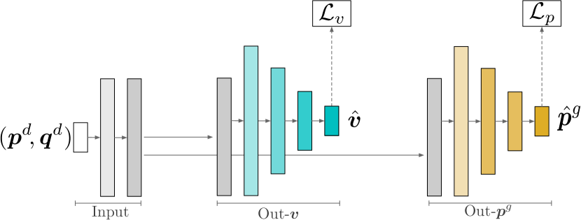
Figure 4: A representation of the AC-OPF Neural Network Model ${\cal M}_{\text{B}}$. Each layer is fully connected with ReLU activation. White boxes correspond to input tensors, dark, colored, boxes correspond to output layers. Loss components are shown in the rectangles with black borders.

Model ${\cal M}_{\text{C}}$

This model exploits the OPF problem constraints using the Lagrangian framework under violation degrees. The model minimizes the following loss:

$${\cal L}_{o}(\bm{y},\hat{\bm{y}}) =\|\bm{v}-\hat{\bm{v}}\|^{2}+\|\bm{\theta}-\hat{\bm{\theta}}\|^{2}$$

$$+\|\bm{p}^{g}-\hat{\bm{p}}^{g}\|^{2}+\|\bm{q}^{g}-\hat{\bm{q}}^{g}\|^{2}$$

$$+\sum_{c\in{\cal C}}\lambda_{c}\nu_{c}(\bm{\hat{y}})$$

with ${\cal C}$ being the set of the OPF constraints as defined in Model 1, and $\nu_{c}(\bm{\hat{y}})$ represent the constraint penalty associated to constraint $c\in{\cal C}$. All weights $\lambda_{c}$ are set to $1$.

Its architecture is summarized in the following table:

Alias	Layer	size in	size out	AF
Input	FC	$2l$	$4l$	ReLU
	FC	$4l$	$4l$	ReLU
Out-$\bm{v}$	FC	$4l$	$8l$	ReLU
	FC	$8l$	$4l$	ReLU
	FC	$4l$	$2n$	ReLU
	FC	$2n$	$n$
Out-$\bm{\theta}$	FC	$4l$	$8l$	ReLU
	FC	$8l$	$4l$	ReLU
	FC	$4l$	$2n$	ReLU
	FC	$2n$	$n$
Out-$\bm{p}^{g}$	FC	$4l$	$8l$	ReLU
	FC	$8l$	$4l$	ReLU
	FC	$4l$	$2g$	ReLU
	FC	$2g$	$g$
Out-$\bm{q}^{g}$	FC	$4l$	$8l$	ReLU
	FC	$8l$	$4l$	ReLU
	FC	$4l$	$2g$	ReLU
	FC	$2g$	$g$

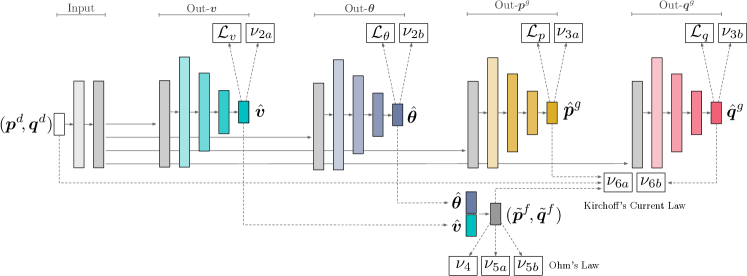
Figure 5: A representation of the AC-OPF DNN model ${\cal M}_{\text{C}}$. White boxes correspond to input tensors, dark, colored, boxes correspond to output layers. Loss components and violation degrees are shown in the rectangles with black borders.

An illustration of the above architecture is provided in Figure 5. The input layers on the left process the tensor of loads $(\bm{p}^{d},\bm{q}^{d})$. The network has four basic units, each following a decoder-encoder structure and composed by a number of layers as outlined in the table above. Each subnetwork predicts a target variable: voltage magnitudes $\hat{\bm{v}}$, phase angles $\hat{\bm{\theta}}$, active power generations $\hat{\bm{p}}^{g}$, and reactive power generations $\hat{\bm{q}}^{g}$. Each sub-network takes as input the last hidden layer of its input subnetwork, that processes the load tensors. Each of the four prediction outputs is used to compute the penalties associated to the quantity bounds ($\nu_{2a}$ for the voltage magnitudes, $\nu_{2b}$ for voltage angles, $\nu_{3a}$ for the active generator power, and $\nu_{3b}$ for the reactive generator power). The predictions for the voltage magnitude $\hat{\bm{v}}$ and angle $\hat{\bm{\theta}}$ are used to compute the load flows $(\tilde{\bm{p}}^{f},\tilde{\bm{q}}^{f})$, as illustrated on the bottom of the Figure and produce penalties $\nu_{4},\nu_{5a},$ and $\nu_{5b}$. Finally, the resulting flows $(\tilde{\bm{p}}^{f},\tilde{\bm{q}}^{f})$ and the predictions for active $\hat{\bm{p}}^{g}$ and reactive $\hat{\bm{q}}^{g}$ generator power are used to compute the penalties associated to the Kirchhoff’s Current Law ($\nu_{6a}$ and $\nu_{6b}$).

Model ${\cal M}_{\text{C}}^{\text{D}}$

This model extends ${\cal M}_{\text{C}}$ by estimating the Lagrangian weights $\lambda_{c}$ using the iterative Lagrangian dual scheme described in Algorithm 1. Its loss function and architecture are analogous to those of model ${\cal M}_{\text{C}}$.

Model ${\cal M}_{\text{CS}}$

This model extend ${\cal M}_{\text{C}}$ by exploiting both the problem constraints and the previous power system state; It uses the same loss function as that used by ${\cal M}_{\text{C}}$ but it adopts the architecture outlined in Figure 1, that uses the information related to the previous power network state, as input to each of the four output subnetwork, in addition to the last hidden layer of the input subnetwork that processes the load tensors.

Its architecture is summarized in the following table:

Alias	Layer	size in	size out	AF
Input	FC	$4l$	$8l$	ReLU
	FC	$8l$	$8l$	ReLU
Out-$\bm{v}$	FC	$8l+n$	$16l+2n$	ReLU
	FC	$16l+2n$	$8l+n$	ReLU
	FC	$8l+n$	$4n$	ReLU
	FC	$4n$	$2n$	ReLU
	FC	$2n$	$n$
Out-$\bm{\theta}$	FC	$8l+n$	$16l+2n$	ReLU
	FC	$16l+2n$	$8l+n$	ReLU
	FC	$8l+n$	$4n$	ReLU
	FC	$4n$	$2n$	ReLU
	FC	$2n$	$n$
Out-$\bm{p}^{g}$	FC	$8l+g$	$16l+2g$	ReLU
	FC	$16l+2g$	$8l+g$	ReLU
	FC	$8l+g$	$4g$	ReLU
	FC	$4g$	$2g$	ReLU
	FC	$2g$	$g$
Out-$\bm{q}^{g}$	FC	$8l+g$	$16l+2g$	ReLU
	FC	$16l+2g$	$8l+g$	ReLU
	FC	$8l+g$	$4g$	ReLU
	FC	$4g$	$2g$	ReLU
	FC	$2g$	$g$

Model ${\cal M}_{\text{CS}}^{\text{L}}$

This model extends ${\cal M}_{\text{CS}}$ by using trainable Lagrangian multipliers $\lambda_{c}$ associated to each constraint penalty $\nu_{c}$, for $c\in{\cal C}$, whose value is learned during the training cycle. Its loss function is thus:

$${\cal L}_{o}(\bm{y},\hat{\bm{y}}) =\|\bm{v}-\hat{\bm{v}}\|^{2}+\|\bm{\theta}-\hat{\bm{\theta}}\|^{2}$$

$$+\|\bm{p}^{g}-\hat{\bm{p}}^{g}\|^{2}+\|\bm{q}^{g}-\hat{\bm{q}}^{g}\|^{2}$$

$$+\sum_{c\in{\cal C}}\lambda_{c}\nu_{c}(\bm{\hat{y}})$$

${\cal M}_{\text{CS}}^{\text{L}}$ has the same network architecture that the one adopted by ${\cal M}_{\text{CS}}$.

Model ${\cal M}_{\text{CS}}^{\text{D}}$

Finally, ${\cal M}_{\text{CS}}^{\text{D}}$, (aka OPF-DNN) uses a different approach to estimate the Lagrangian weights $\lambda_{c}$: It does so by using the iterative Lagrangian dual scheme described in Algorithm 1. Its loss function and architecture are analogous to those of model ${\cal M}_{\text{CS}}^{\text{L}}$.

References

- [Anwar, El Moursi, and Xiao 2016] Anwar, M. B.; El Moursi, M. S.; and Xiao, W. 2016. Novel power smoothing and generation scheduling strategies for a hybrid wind and marine current turbine system. IEEE Transactions on Power Systems 32(2):1315–1326.
- [Arteaga et al. 2019] Arteaga, J. H.; Hancharou, F.; Thams, F.; and Chatzivasileiadis, S. 2019. Deep learning for power system security assessment. In 2019 IEEE Milan PowerTech.
- [Baran and Wu 1989] Baran, M. E., and Wu, F. F. 1989. Optimal capacitor placement on radial distribution systems. IEEE Transactions on Power Delivery 4(1):725–734.
- [Boukelia, Arslan, and Mecibah 2017] Boukelia, T.; Arslan, O.; and Mecibah, M. 2017. Potential assessment of a parabolic trough solar thermal power plant considering hourly analysis: ANN-based approach. Renewable Energy 105:324 – 333.
- [Chatziagorakis et al. 2016] Chatziagorakis, P.; Ziogou, C.; Elmasides, C.; Sirakoulis, G. C.; Karafyllidis, I.; Andreadis, I.; Georgoulas, N.; Giaouris, D.; Papadopoulos, A. I.; Ipsakis, D.; Papadopoulou, S.; Seferlis, P.; Stergiopoulos, F.; and Voutetakis, S. 2016. Enhancement of hybrid renewable energy systems control with neural networks applied to weather forecasting: the case of Olvio. Neural Computing and Applications 27(5):1093–1118.
- [Chowdhury and Rahman 1990] Chowdhury, B. H., and Rahman, S. 1990. A review of recent advances in economic dispatch. IEEE Transactions on Power Systems 5(4):1248–1259.
- [Coffrin et al. 2018] Coffrin, C.; Bent, R.; Sundar, K.; Ng, Y.; and Lubin, M. 2018. Powermodels.jl: An open-source framework for exploring power flow formulations. In PSCC.
- [Coffrin, Gordon, and Scott 2014] Coffrin, C.; Gordon, D.; and Scott, P. 2014. NESTA, the NICTA energy system test case archive. CoRR abs/1411.0359.
- [Deka and Misra 2019] Deka, D., and Misra, S. 2019. Learning for DC-OPF: Classifying active sets using neural nets. In 2019 IEEE Milan PowerTech.
- [Deutche-Energue-Agentur 2019] Deutche-Energue-Agentur. 2019. The e-highway2050 project. http://www.e-highway2050.eu. Accessed: 2019-11-19.
- [Donnot et al. 2019] Donnot, B.; Donon, B.; Guyon, I.; Liu, Z.; Marot, A.; Panciatici, P.; and Schoenauer, M. 2019. LEAP nets for power grid perturbations. In European Symposium on Artificial Neural Networks.
- [Fioretto, Mak, and Van Hentenryck 2020] Fioretto, F.; Mak, T. W. K.; and Van Hentenryck, P. 2020. Predicting AC optimal power flows: Combining deep learning and lagrangian dual methods. In Proceedings of the AAAI Conference on Artificial Intelligence (AAAI), to appear.
- [Fisher, O’Neill, and Ferris 2008] Fisher, E. B.; O’Neill, R. P.; and Ferris, M. C. 2008. Optimal transmission switching. IEEE Transactions on Power Systems 23(3):1346–1355.
- [Fontaine, Laurent, and Van Hentenryck 2014] Fontaine, D.; Laurent, M.; and Van Hentenryck, P. 2014. Constraint-based lagrangian relaxation. In Principles and Practice of Constraint Programming, 324–339.
- [Hestenes 1969] Hestenes, M. R. 1969. Multiplier and gradient methods. Journal of optimization theory and applications 4(5):303–320.
- [Ince et al. 2016] Ince, T.; Kiranyaz, S.; Eren, L.; Askar, M.; and Gabbouj, M. 2016. Real-time motor fault detection by 1-D convolutional neural networks. IEEE Transactions on Industrial Electronics 63(11):7067–7075.
- [LeCun, Bengio, and Hinton 2015] LeCun, Y.; Bengio, Y.; and Hinton, G. 2015. Deep learning. Nature 521:436–444.
- [Liu et al. 2018] Liu, J.; Marecek, J.; Simonetta, A.; and Takač, M. 2018. A coordinate-descent algorithm for tracking solutions in time-varying optimal power flows. In Power Systems Computation Conference.
- [Monticelli, Pereira, and Granville 1987] Monticelli, A.; Pereira, M.; and Granville, S. 1987. Security-constrained optimal power flow with post-contingency corrective rescheduling. IEEE Transactions on Power Systems 2(1):175–180.
- [Ng et al. 2018] Ng, Y.; Misra, S.; Roald, L.; and Backhaus, S. 2018. Statistical learning for DC optimal power flow. In Power Systems Computation Conference.
- [Niharika, Verma, and Mukherjee 2016] Niharika; Verma, S.; and Mukherjee, V. 2016. Transmission expansion planning: A review. In International Conference on Energy Efficient Technologies for Sustainability, 350–355.
- [Pache et al. 2015] Pache, C.; Maeght, J.; Seguinot, B.; Zani, A.; Lumbreras, S.; Ramos, A.; Agapoff, S.; Warland, L.; Rouco, L.; and Panciatici, P. 2015. Enhanced pan-european transmission planning methodology. In IEEE Power Energy Society General Meeting.
- [Paszke et al. 2017] Paszke, A.; Gross, S.; Chintala, S.; Chanan, G.; Yang, E.; DeVito, Z.; Lin, Z.; Desmaison, A.; Antiga, L.; and Lerer, A. 2017. Automatic differentiation in pytorch. In NIPS-W.
- [Tang, Dvijotham, and Low 2017] Tang, Y.; Dvijotham, K.; and Low, S. 2017. Real-time optimal power flow. IEEE Transactions on Smart Grid 8(6):2963–2973.
- [Tong and Ni 2011] Tong, J., and Ni, H. 2011. Look-ahead multi-time frame generator control and dispatch method in PJM real time operations. In IEEE Power and Energy Society General Meeting.
- [Wächter and Biegler 2006] Wächter, A., and Biegler, L. T. 2006. On the implementation of an interior-point filter line-search algorithm for large-scale nonlinear programming. Mathematical Programming 106(1):25–57.
- [Wang, Shahidehpour, and Li 2008] Wang, J.; Shahidehpour, M.; and Li, Z. 2008. Security-constrained unit commitment with volatile wind power generation. IEEE Transactions on Power Systems 23(3):1319–1327.
- [Wood and Wollenberg 1996] Wood, A. J., and Wollenberg, B. F. 1996. Power Generation, Operation, and Control. Wiley-Interscience.