Overtone Pulsations Revisited

Abstract

The shape of light cures of fundamental-mode and of first-overtone pulsators, as observed in RR Lyrae variables and Cepheids, differ characteristically. The stellar physical origin of the morphological differences is not well documented and the topic seems not to be part of the elementary curriculum of students of stellar variability. To ameliorate the situation, this exposition analyzes hydrodynamical simulations of radial pulsations computed with the newly available numerical instrument RSP in MESA. The stellar physical processes that affect the light curves are identified and contrasted to the explanation based on experiments with one-zone models. The encounter of first-overtone pulsators sporting light curves that mimic those of fundamental-mode variables serves as a warning that light-curve morphology alone is not a reliable path to correctly classify pulsating variables; the exposition closes with a short discussion of constraints these modes might impose on understanding the origin of anomalous Cepheids.

CBmA, 4410 Liestal, Switzerland

1 Introduction

Temporal variability of celestial objects was and still is mainly detected by measuring their brightness changes. The time-scale of the variability together with the form of the temporal brightness change – the light curve – serve as the basic initial criteria to classify an object’s variability. Reliable classifications, in particular ones which can be quantified and attributed automatically by software tools is gaining importance in the age of petabyte data-generating sky surveys.

In the study of pulsating variable stars, Fourier decomposition of light curves has proved useful (Schaltenbrand & Tammann, 1971). Amplitude ratios and phase differences of low-order components of invoked Fourier series (e.g. Simon & Lee, 1981) are used to capture pertinent features of the light curves aiming at a robust classification of variable stars. For a long time stellar-pulsation researchers even hoped that amplitude ratios and phase differences can be correlated with physical processes that operate in the interior of pulsating variables. Success was, however, partial at best.

Stellingwerf & Donohoe (1987) introduced a coarse-grained light-curve characterization via the concepts of Skewness (Sk) and Acuteness (Ac).[][-1.5 cm] Sk $\doteq 1/\Delta\phi_{\mathrm{rb}}-1$ with $\Delta\phi_{\mathrm{rb}}$ measuring the fraction of the pulsation period taken up by the rising branch of the light curve. Ac $\doteq 1/\Delta\phi_{\mathrm{fw}}-1$ where $\Delta\phi_{\mathrm{fw}}$ measures the time (in units of the star’s pulsation period) during which the variable star stays above its mean brightness. Therefore, Ac is a full-width-at-half-maximum measure of the light curve. Based on simple nonlinear modeling behavior, the quantity Sk was observed to correlate with the nonlinearity of the pulsation velocity whereas Ac was claimed to depend on the light amplitude at the base of the pulsation driving region. Since stellar pulsations are examples of thermo-mechanical oscillators it is likely that Ac and Sk are not independent of each other. Both quantifiers have been shown to correlate with low-order Fourier components but they are less sensitive measures of light-curve forms than Fourier phases and amplitude ratios (Stellingwerf & Donohoe, 1987). Irrespective of any physical interpretation of Sk and Ac, here they serve as useful morphological quantifiers in our endeavor to understand the Grundform[][-0cm]in the sense of the uncarved block that captures the constitutive shape already but does not yet reproduce elaborate overlying details of light curves of F- and 1O-mode pulsators.

Even before the RR Lyrae variable stars were baptized as such and even before their having been recognized as a class they were abundantly observed globular clusters: In a study of the variable stars in $\omega$ Cen, Bailey (1902) realized that the cluster variables, as the RR Lyr variables were referred to then, come in more than one flavor. Guided by their periods, light-variation amplitude, and the form of the light curves, Bailey subdivided the cluster variables into two longer-period, higher-amplitude groups with asymmetric light curves, which he termed RRa ($0.5\lesssim P/{\mathrm{d}}\lesssim 0.66$), cf. upper light curve in Fig. 1, RRb ($0.66\lesssim P/{\mathrm{d}}\lesssim 0.9$ and light curves somewhat less acute than those of RRa variables) stars, and shorter-period ($0.3\lesssim P/{\mathrm{d}}\lesssim 0.5$), lower-amplitude variables with almost sinusoidal light curve shapes, were referred to as the RRc subclass, cf. lower light curve in Fig. 1. When Schwarzschild (1940) analyzed cluster-variable data of M3 he speculated that RRc variables are first-overtone (1O) and the RRa and the RRb variables (conveniently fused to RRab) fundamental-mode (F) radially pulsating stars. This conjecture was later confirmed: Baker (1965) presented results of linear stability analyses where 1O and F modes were excited simultaneously over essentially the full width of the instability strip. In the same conference proceedings, Christy (1965) discussed his early nonlinear hydrodynamical computations of RRab and RRc variables. The light-curve shapes of the RRab models agreed well with observations. The quality of the bolometric RRc light curves was, however, low; despite being less skew than F-mode light curves they lacked the low acuteness and the smoothness that characterize RRc variables. The situation improved markedly only toward the end of the last millennium (e.g. Feuchtinger, 1999, and references therein).

Light curves in the photometric I band of RR Lyrae variables observed during the OGLE sky monitoring program. Top: RRab with Sk$=5.9$, Ac$=1.8$. Bottom: RRc with Sk$=1.4$, Ac$=0.8$.

Despite some early successes to model hydrodynamically RR Lyr variables pulsating in their F- and 1O-mode, respectively, a solid explanation of their characteristically differing light curves was lacking. Stellingwerf et al. (1987) resorted to the concept of one-zone models (OZM) in which the most important physics is boiled into parameters whose impact can be easily studied with simplified nonlinear differential equations. Emphasizing the effect of the spatial node of 1O modes on the luminosity that enters the pulsating "zone" of the OZM led Stellingwerf et al. (1987) to conclude that it is the phase reversal, relative to the luminosity variation inside the pulsating shell, of the energy flux entering the pulsation zone from the sub-node interior that effects the sinusoidal light curves of RRc stars. Taking the idea one mode order further, Stellingwerf et al. even speculated on how the light curves of RRe variables, i.e. RR Lyr – type variables pulsating in their second overtone mode, should look like.

Hydrodynamical modeling of radially pulsating stars has recently become more widely accessible (Paxton et al., 2019), the CPU power of even modest computers together with significantly broadened visualization possibilities led to this exposition that attempts to eventually check if the conclusions put forth in Stellingwerf et al. (1987) can be recovered in full hydrodynamical simulations. In a first step, RR Lyr models are addressed. The analyses are carried over to Cepheids in whose short-period domain F and 1O modes can again be excited simultaneously so that different pulsation modes can be studied in the same envelope models, so that structural differences are eliminated that might affect pulsation modes when models with different stellar parameters need to be invoked. This exposition also addresses the light curves of second-overtone pulsations, at least in the case of Cepheid models and finally discusses the surprising sighting of an 1O pulsator that masquerades as an F-mode and its consequences.

2 RR Lyrae variables

Using the RSP  (Smolec & Moskalik, 2008) instrument of MESA, a representative RR Lyrae variable envelope model was computed: The adopted stellar parameters were $0.65\,M_{\odot}$ at $45\,L_{\odot}$ and $T_{\rm eff}=6900$ K with a chemically homogeneous composition of $X=0.75,Z=0.0014$. The inner boundary of the envelope, where the pulsation velocity is assumed to vanish and where a constant energy flux enters from the stellar interior, was set at $2\times 10^{6}$ K. The envelope was subdivided into $230$ zones, with $80$ zones located at temperatures below $11\cdot 10^{3}$ K in the hydrostatic starting model.

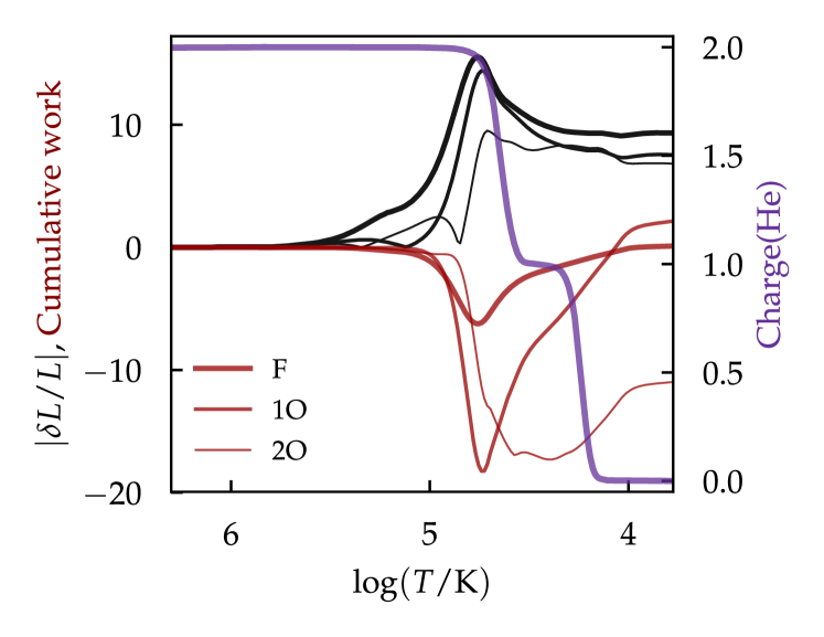
Figure 1: LNA results of the lowest three radial pulsation modes (coded by line thickness) of the RR Lyrae model. Temperature measures the depth in the model’s envelope. The relative luminosity perturbation is plotted with black lines. The cumulative work done by the envelope is coded in red. For orientation, the indigo line traces the average charge of helium atoms in the envelope.

Linear nonadiabatic (LNA) stability analysis of the hydrostatic initial model revealed the RRab-like fundamental (F) mode and the RRc-like first overtone (1O) mode to be both unstable. This allowed for the study of saturated nonlinear F and O1 pulsations of the same envelope model. Figure 1 displays pertinent quantities from the LNA analysis of the RR Lyr – type model: The black lines trace the spatial variation of the magnitude of the relative luminosity perturbation eigenfunctions $|\delta L/L|$ of the lowest three radial orders. The legend in the lower left corner of the plot specifies the meaning of the line thickness used for the eigendata. The red lines trace the spatial structure of the cumulative work done by the respective pulsation modes when integrating from the base of the envelope. A positive value at the outer (right) boundary means that the respective mode is excited (as it applies for F and 1O modes of the model shown in Fig. 1). The remaining thick indigo-colored line measures the average charge of the helium atoms in the envelope. The rise of the average He-charge from 0 to 1 at about $4.15<\log T<4.4$ traces the first partial ionization zone (PIZ) of helium (HeI). At slightly lower temperatures lies the PIZ of hydrogen. The HeII PIZ, with the average charge of helium changing from 1 to 2, spans the region of $4.55<\log T<4.8$.

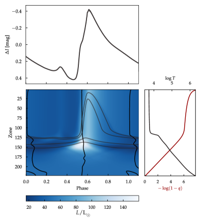
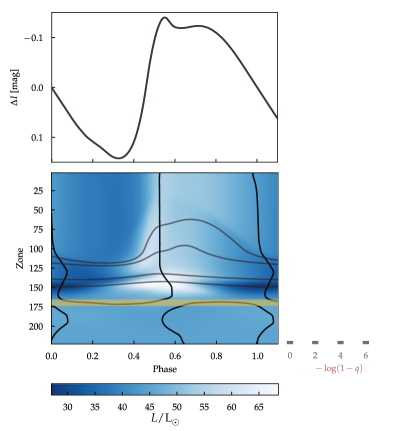
Figure 2: Triptycha composed of two pulsation panels on top of each other and a structure panel on the bottom right for the RRab (left, $P=0.4560$ d) and the RRc (right, $P=0.3361$ d) model.

The particular nonlinear mode aimed at in the direct integration of the nonlinear hydro equations can frequently be selected initially by imposing the appropriate LNA velocity eigenfunction as the perturbation of the static start model (cf. MESA  instrument paper Paxton et al., 2019, e.g. their Sect. 2.4.6 and references therein). Both, F and 1O modes could be successfully followed into their respective limit cycles. Selected behavior of radial pulsations of the RRab- and RRc-type pulsations that have reached their respective limit cycles is depicted in Fig. 2 Both triptycha are composed in the same way: The central frame is the color coded spatio-temporal bolometric luminosity variation over $1.2$ pulsation cycles; phase $=0$ is set at the epoch of maximum photospheric radius. The simulations’ zone number serves as the spatial coordinate. The counting starts at the stellar surface. Because the RSP instrument is a lagrangian hydro code, zone numbers map onto a temporally invariant fixed-mass gridding. The color coding of the luminosity variation, in units of solar luminosity, is resolved a the bottom of the frame. The thick black lines trace the contour of $v_{\mathrm{puls}}=0$. Both triptycha show that the phases of maximum and minimum radius shift as a function of depth in the envelope. The considerable shifts close to the inner boundary of the envelopes are likely affected by interpolation uncertainties at the very small pulsation amplitudes in the deep interior. The colormesh plot of the RRc-like pulsation in the right-hand triptychon of Fig. 2 was augmented with a transparent yellow line tracing the essentially horizontal parts of $v_{\mathrm{puls}}=0$ loci. This spatially invariant line approximates well the position of the 1O pulsation mode’s node (which is also seen at about $\log T=5$ in the luminosity perturbation of the LNA analysis shown in Fig. 1). Four weaker grey lines on top of the colormesh plots trace the mass depth of the two helium PIZs; the lines trace the average He charge of $1.9,1.1$ (HeII PIZ) and higher up in the envelope $0.9,0.1$ (HeI PIZ), respectively.

To get an impression of what the zone numbers mean physically, the plot panels in the lower right of the triptycha quantify the temporally invariant mass stratification (with $q\doteq m/M_{\ast}$ ) in red and the temperature stratification at phase $=0$ (black line). The emergent light curve in the photometric $I$-band of the saturated pulsation mode is plotted on top of the color frame, both panels span $1.2$ pulsation cycles.The $I$-band magnitudes were computed requesting log_lum_band bb_I in MESA’s history_columns.list; the "bb" option assumes the stellar radiation field to be a blackbody with the model’s effective temperature to compute the bolometric correction.

Most evidently, both colormesh frames of Fig. 2 show that the global maximum luminosity is not radiated from the stellar surface but is attained deeper in the stellar envelope. This property is, of course, also recovered in the LNA analyses (cf. Fig. 1). The pile-up of the star’s energy flux happens in layers where helium goes from twice to once ionized. Figure 2 illustrates that also the darkest patches (lowest luminosities) are encountered at about the hotter end the HeII PIZ. This observation of the luminosity behavior applies to both, the RRab and the RRc models. In contrast to the F mode, the 1O pulsator experiences, however, a comparatively longer high-luminosity phase. The computations show that the luminosity blocking effect that takes place at the base of the HeII PIZ broadly shapes, albeit somewhat smoothed out, the emergent surface luminosity variation. Hence, what happens at the base of the HeII PIZ governs the Grundform of the observable light curve, and it is the quantity Ac, which is affected in particular.

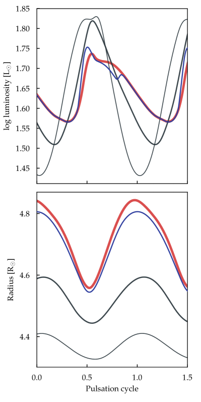
Figure 3: Top: Comparison of the bolometric surface luminosity (red), the luminosity variation at the H/HeI (blue) and the HeII PIZ (cool edge heavier grey and hot edge thinner grey line) for RRab (left) and RRc model (right). Bottom: Respective radius variation; color coding is the same as in the top panels.

Resorting to the physical reasoning of Cox & Giuli (1968, in Ch. 27.6 + 27.7), in the linear quasi-adiabatic approximation applied to radiative regions it is found that $\delta L/L\sim\left(\Gamma_{3}-1\right)\delta\rho/\!\rho$ and $\sim{\mathrm{d}}_{x}\left(\left(\Gamma_{3}-1\right)\delta\rho/\!\rho\right)$.[][-0.0cm] Notice: $\delta\rho/\rho=-3\,\delta r/r-x\,{\mathrm{d}}_{x}\left(\delta r/r\right)$ with $\delta$ denoting a Lagrangian perturbation and $x\doteq r/R_{\ast}$. Before a PIZ is encountered radiative dissipation ($\delta L/L$ rising outwards in Fig. 1) grows with the density- and hence the radius-variation amplitude of the pulsation. Once a PIZ develops, $\Gamma_{3}-1$ drops and so does $\delta L/L$ accordingly. Hence, the blocking of the energy flux at the bottom of the HeII PIZ depends on the time span over which the density is appropriately enhanced there. Figure 3 illustrates the correlation of the luminosity variation as a function of depth in the stellar envelopes together with the associated radius variations for RRab (left) and RRc (right) models, respectively. The top two panels show the bolometric luminosities emerging from the photosphere (red line), the luminosity variation obtaining at the H/HeI-ionization zones (blue line), at the cool end of the HeII PIZ (thicker grey line), and finally at the hot edge of the HeII PIZ (thinner grey line). [][-2.0cm]The luminosity variations of the RRab model yield: Location Sk Ac surface 5.7 2.0 H/HeI PI 5.7 2.0 HeII PI, cool 2.3 3.2 HeII PI, hot 2.0 2.2

the RRc model yields: Location Sk Ac surface 3.2 1.1 H/HeI PI 3.8 1.0 HeII PI, cool 1.5 1.3 HeII PI, hot 0.6 1.0 The lower two panels contain the corresponding radius variations at the same mass depths, using the same line scheme. Evidently, for the RRab case on the left, the compression phase appears considerably narrower – looking more like a bounce – when compared with the sinusoidal lines belonging to both edges of the HeII PIZ. The emerging light curves pick up their rough form from what happens at the HeII PIZ. In case of the RRc model, the sharp peak that emerges at the end of the ascending branch is contributed by the H/HeI PIZ. The reason of the more harmonic motion of the HeII PIZ in the RRc case can be attributed to the presence of the node at about $\log T=5$. The proximity of the node inflicts a comparatively lower pulsation amplitude but a comparatively longer duration of compression at the hot end of the HeII PIZ so that the nonlinearities are less expressed than in the unconfined F mode.

Sidenote 3 tabulates the variation of the quantities Ac and Sk at various depths of the model envelopes. The skewness of the RRab model doubles when going from the base of the HeII PIZ to the photosphere; the variation of the acuteness, on the other hand, does not change significantly. In the case of the F-mode pulsator, the action of the H/HeI PIZ steepens considerably the ascending branch of the light curve. A similar behavior, with different numerical values for the quantities Sk and Ac, is observed in the RRc model. Most importantly, the RRc’s photospherical Sk value is much higher than what is observed in nature. This is caused by the sharp bump that is picked up across the H/HeI PIZ by the O1 pulsator. Because the bump that appears in our modeled case exceeds maximum light of the Grundform, the magnitude of Sk overshoots accordingly. If the maximum seen in the red-colored light curve in the upper right of Fig. 3 were weaker and would not count as the global light maximum then the skewness would drop to a moderate Sk = 1.8, which compares favorably with what is observed say in the OGLE RRc case shown Fig. 1.

[-5.2cm]

Convective strength, measured as convective luminosity in units of the local total stellar luminosity as a function of depth in the envelope and of pulsation phase for the RRab (top) and the RRc model (bottom). For the RRab case, the quantities Ac and Sk of the model reproduce well what is observed. RRc models reproduce the magnitude of the observed Ac values. The skewness, on the other hand depends strongly on the strength of a bump along the ascending light branch the models pick up across the He/HeII PIZ. Across this region, the star’s energy is mainly transported by convection (see Fig. 3). Strength and even position of such bumps are affected by the details of the time-dependent convection modeling, i.e. by the choice of the parameters entering the RSP computations. Since the convection-model parameters are usually weakly confined by theory, playing with them can be used to find better agreement with observations.

Looking at the RRc triptychon of Fig. 2, it is important to notice that the luminosity variation below (at lower mass) the 1O node is small or even negligible.[][-2.2cm]The same conclusion be drawn, of course, upon inspecting Fig. 1 Hence, the effect of the phase change of the luminosity variation across the node is not pertinent for the pulsation.

3 Cepheid variables

[-1.3cm]

Light curves in the photometric $I$-band of Cepheid variables observed in the SMC during the OGLE monitoring program. Top: F-mode with Sk = 3.0, Ac = 1.3. Bottom: 1O-mode with Sk = 1.3, Ac = 1.0. The previous section addressed the differences in the luminosity variation at the bottom of the helium PIZs of RRab and RRc pulsators. In this section we want to learn how the findings for RR Lyrae variables carry over to the more massive, more luminous Cepheids. For this, we chose again an appropriate model star to describe a Cepheid whose fundamental and first overtone radial modes are both pulsationally unstable. The stellar parameters of the Cepheid model are: $4.17\,M_{\odot}$ at $1439\,L_{\odot}$ and $T_{\rm eff}=6050$ K. The envelope is assumed to be chemically homogeneous with SMC-compatible abundances of $X=0.75,Z=0.004$. The Cepheid’s envelope was subdivided into $300$ zones, with $80$ zones located at temperatures below $11\cdot 10^{3}$ K of the hydrostatic initial model.

Figure 4 depicts the LNA results for the lowest three radial modes of the short-period Cepheid model. The meaning of the lines is the same as in Fig. 1. As mentioned before, the F- and the 1O modes are unstable. The growth rate of the 1O-mode exceeds that of the F-mode. As in the RR Lyrae case, the node of the 1O mode lies at about $\log T=5$ of the starting model.

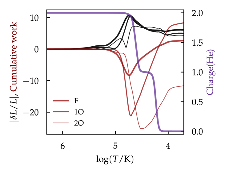
Figure 4: LNA results of the lowest three radial pulsation modes (coded by line thickness) of the Cepheid model. Temperature measures the depth in the model’s envelope. The relative luminosity perturbation is plotted with black lines. The cumulative work done by the envelope is coded in red. For orientation, the indigo line traces the average charge of helium ions in the envelope.

The RSP computations on the Cepheid model were started with pure F or 1O LNA velocity eigenfunctions whose amplitudes were set to $0.1$ km/s at the model surface. The F-mode pulsation took about 3500 cycles before it reached its limit-cycle with a period of $3.93925$ d, which agrees with the LNA period up to five digits. Even though the simulation was started with a pure LNA F-eigenmode the pulsations developed, between 1500 and 8000 d, a long mixed-mode phase (F and 1O-mode) with an upper envelope of the pulsation amplitude at about $\Delta M_{\mathrm{bol}}=0.4$ before the pure F-mode took over eventually and saturated at an amplitude of about $\Delta M_{\mathrm{bol}}=1.1$. The resulting light curve in the photometric $I$-band is shown in the top frame of the left triptychon in Fig. 5. The quantities plotted in the three frames are the same as in Fig. 2. The F-mode’s I-band Grundform parameters are Ac = 1.1 and Sk = 3.5, both of which compare well with the respective observed quantities derived for the case shown in Fig. 3. Also the luminosity behavior displayed in the colormesh frame is comparable to the RRab situation.

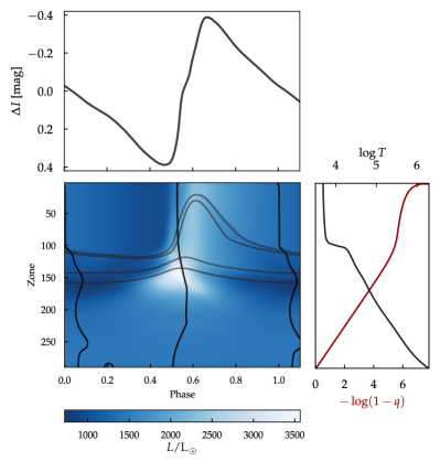
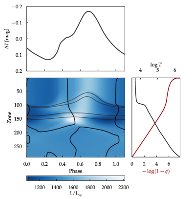
Figure 5: Triptycha of the same kind as shown in Fig. 2 for the F-mode with $P=3.9325$ d (left) and the 1O-mode with $P=2.83263$ d (right) Cepheid model.

After perturbing the hydrostatic Cepheid model with the 1O velocity eigenvector the pulsation grew exponentially into a pure 1O pulsation, which saturated at an amplitude of $\Delta M_{\mathrm{bol}}=0.4$ after about 1000 days. The corresponding $I$-band light curve is displayed as the top frame of the right triptychon in Fig. 5. The final nonlinear pulsation period of $2.83263$ d is only 1 ‰ longer than the corresponding LNA value. The magnitudes of the Grundform-characterizing quantities Sk = 1.3 and Ac = 1.6 fare decently well in comparison with the observed values for the 1O case shown in Fig. 3. The bump at the lower ascending branch of the $I$-band light curve, however, hints already at the impact its position and/or amplitude can have on the magnitude of the quantity Ac. In the case of the 1O Cepheid the full width at half maximum to quantify Ac happens to lie just above the shoulder of the ascending-branch bump. With a bump that occurred slightly higher, Ac would drop to unity or even lower. The observed 1O Cepheid, OGLE-SMC-CEP-4139, shows also a bump after minimum light, its expression is, however, less pronounced than that of the simulation. From the colormesh diagram it is evident that the bump grows out of processes acting in the H/He PIZ so that details of this bump are prone to particular choices of convective parameters that characterize the coupling of the turbulent energy transport with the pulsating environment. The more or less horizontal components of the $v_{\mathrm{puls}}=0$ curves in the colormesh diagram of the 1O mode trace the location of the pulsation mode’s node. In contrast to the RRc case, the position of the $v_{\mathrm{puls}}$ node is not constant in zones, and hence not constant in mass. The cyclic motion in mass is not large but noticeable anyway.

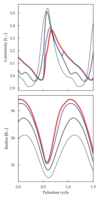
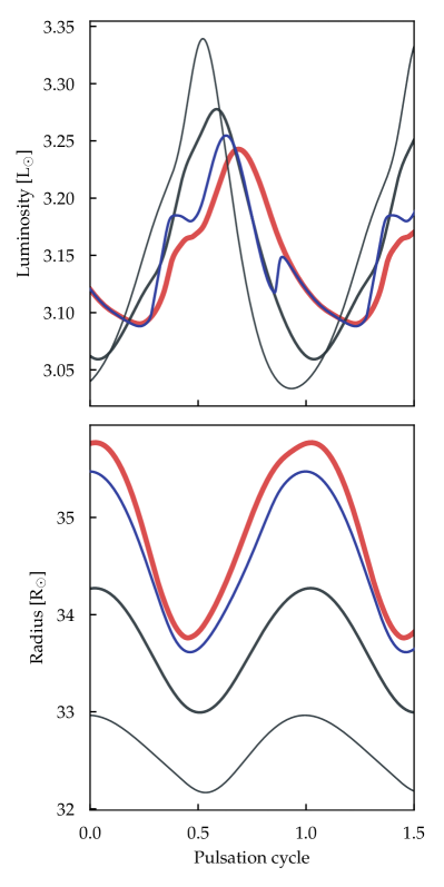
Figure 6: Top: Comparison of the bolometric surface luminosity (red), the luminosity variation at the H/He (blue) and the HeII PIZ (heavier grey for the cool edge and thinner grey line for the hot edge ) for F- (left) and 1O-mode Cepheid (right). Bottom: Respective radius variation; color coding is the same as in the top panels.

[-6.8cm] Mode Sk Ac F 3.5 1.1 1O 1.3 1.6 Figure 6 illustrates how the luminosity and the radius varies at selected mass-depths through the envelope of the Cepheid model. As in Fig. 3 for the RR Lyrae model, the red line traces the variation at the photosphere, the blue line at the H/He PIZ, the thick grey line at cool end and the thin line at the hot end of the HeII PIZ. Comparing Fig. 6 with Fig. 3 reveals that the Cepheid’s F and 1O-mode behave much like those in the RR Lyrae-variable model: The amplitudes of the bolometric luminosity variation shrink with increasing mass. The Grundform of the light curve is already carved out at the level of the HeII PIZ. Across the H/He PIZ, temporally well confined bumps and/or dips develop, which are eventually somewhat smeared out when they emerge at the photosphere. The radius variation of the F mode appears again more nonlinear with a sharp, bouncing episode around phase $=0.6$ than the smoother more sinusoidal-looking behavior of the 1O mode.

4 Discussion

The nonlinear hydrodynamical radial-pulsation instrument called RSP  in the recently released MESA  version (Paxton et al., 2019) allows to study in detail fundamental and first overtone pulsations in RR Lyrae and Cepheid model envelopes. Light curves of both pulsation modes could be reproduced satisfactorily.

The Grundform of the light curves, which is quantified by the two parameters skewness, Sk, and acuteness, Ac, can be attributed to the pulsation dynamics, i.e. to the duration of the compression phase, at the base of the HeII PIZ. Already the duration of the imposed luminosity blocking determines the acuteness of the light curve. The Sk-affecting finer details such as bumps and dips along the light curve are influenced or even caused by processes in the H/He PIZ where superadiabatic convection dominates the energy transport in particular during the rising-light phase. Hence, tweaking convection-model parameters, which are theoretically ill constrained, can be used to mold these secondary features into the observationally documented shapes. The RSP instrument constitutes a versatile tool for such data-driven fine-tuning endeavors.

The compression phase of the F-mode pulsators is considerably more confined in time and nonlinear-looking than the more harmonic behavior encountered in 1O pulsators. The latter sinusoidal character is inflicted by the smaller pulsation amplitude at the base of the HeII PIZ due to the proximity of the 1O node at around $10^{5}$ K. Hence, the node of the 1O mode is indeed the cause of the more harmonic 1O light curves; however, it is not the swapped phase relation of the energy flux from below the node as conjectured and modeled via OZMs in Stellingwerf et al. (1987) but the reduced pulsation amplitude in the neighborhood of the node.

The $v_{\mathrm{puls}}=0$ lines in the colormesh frames of the triptycha of Figures 2 and 5 indicate that maximum and minimum radius are not reached at the same phase for all mass depths. The phase of $v_{\mathrm{puls}}=0$ is not even a monotonous function of depth in the envelope. If the velocity nodal line of a 1O mode is added then the situation gets even more intricate: Pulsation phases can be found when up to 6 locations in the envelope have $v_{\mathrm{puls}}=0$. Linear-theory thinking could mislead to interpret such snapshots as a manifestation of a 6O mode. Adhering, however, to a whole-cycle centered view makes it clear that one deals merely with an 1O mode.

Second Overtone Pulsations are a natural conceptual next step to test the effect of the proximity to the HeII PIZ of the top-most node on the Grundform of the light curve. The very existence of 2O modes in RR Lyrae variables in nature has been disputed in the past. The latest compilation of the OGLE RR Lyrae observations in the Magellanic Clouds (Soszyński et al., 2016) attributes to the RRc subclass all the variables that were previously suspected to be 2O pulsators. Furthermore, pulsation modelers never managed to find excited 2O modes for model stars that are compatible with evolutionary scenarios that explain single-star RR Lyr populations (e.g. Kovacs, 1998). In accordance with the older studies also our attempts failed to obtain excited 2O modes over the whole domain that might contain them according to Fig. 1 in Bono & Stellingwerf (1994). Therefore, we focused on Cepheids whose 2O modes are more established, observationally and theoretically. Resorting to the Bono et al. (2001) study, we arbitrarily chose the case of a $3.25\,M_{\odot}$ at $309\,L_{\odot}$ with $T_{\rm eff}=6850$ K star with and a homogeneous envelope composition of $X=0.746,Z=0.004$.

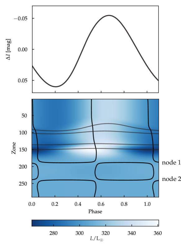
Figure 7: Second-overtone model Cepheid with $3.25M_{\odot}$ after its pulsation saturated with a period of $0.49713$ d. The top panel shows the I-band light curve with the same phasing as the bolometric luminosity colormesh plot on the bottom. The overplotted lines have the same meaning as in Fig. 2.

The LNA analysis showed the 1O and 2O modes to be unstable with the 1O mode only marginally so. After computing through about $10\,000$ cycles, the nonlinear pulsation was well saturated and essentially in its limit cycle with a period of $0.49713$ d. The resulting light curve in the photometric $I$-band is shown in the top frame of Fig. 7 with its small amplitude of about $\Delta I=0.12$ mag. The bottom panel contains again a colormesh plot with the color-coded bolometric luminosity as a function of mass depth and pulsation phase. The black lines trace the loci of $v_{\mathrm{puls}}=0$; the grey lines mark the boundaries of the two helium PIZ as already described for Fig. 2.

The mass depth of the two nodes (referred to as node$\,1$ and node$\,2$ in Fig. 7) of the 2O mode are hinted at on the right side of the colormesh plot. In contrast to the 1O Cepheid case discussed further up, here the essentially perfectly horizontal parts of $v_{\mathrm{puls}}=0$ indicate that the mass depth of both nodes remains constant in time. Furthermore, node 1 lies closer (in mass) to the bottom of the HeII PIZ so that the light curve assumes an even more harmonic form than the 1O brethren. This is very much along the line of reasoning that the proximity of a node to the HeII PIZ sculpts the Grundform of the light curve. As is evident from the colormesh plot, interior to node 1 and even more so to node 2 the luminosity variation is very small and is essentially negligible for the observable pulsation behavior.

F-mode Impostors: A model Cepheid with $3.8M_{\odot}$ at $500L_{\odot}$ and with $T_{\rm eff}=6600$ K was initiated with a 2O mode as obtained from the linear stability analysis. During the first about $2000$ days model time the mode evolved and saturated at about $\Delta\mathrm{M}_{\mathrm{bol}}=0.2$ mag amplitude. Since also the 1O mode is unstable in this model, with about the same growth rate as the 2O mode, some beating developed, which grew stronger over the ensuing roughly $3500$ days. Eventually, the pulsation of the stellar envelope settled at the considerably higher amplitude of $\Delta\mathrm{M}_{\mathrm{bol}}=0.82$ and a period of $0.940$ d, which is very close to the LNA period of the 1O mode. This per se is not surprising, we just witnessed a mode switching from an initialized 2O mode to the apparently physically more attractive 1O mode. The real treat, however, is the final light curve of the 1O mode: The resulting light curve, shown in the top panel of Fig. 8, looks like that of an F-mode pulsator. In the $I$-band, Fig. 8 reveals Sk = 3.0 and Ac = 2.4. The amplitude of the variability ($\Delta I=0.49$ mag) though is about $25\%$ smaller than what a comparable generic F-mode model pulsator develops.

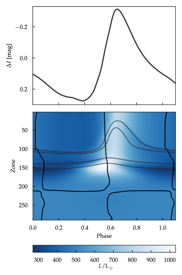
Figure 8: Diptychon of the $3.8M_{\odot}$ Cepheid F-mode impostor pulsating with a period of $0.940$ d. The model pulsates in its 1O mode; except for the amplitude, the light curve, with Sk = 3.0 and Ac = 2.4, compares well with that of an F-mode pulsator.

[-2.5cm]

LNA eigendata for the $3.8M_{\odot}$ Cepheid model. The vertical dashed line marks the position of the luminosity node of the 1O mode at about $\log T=5.34$. The rest of the illustration is the same as in Fig. 1. Also in the F-mode impostor we see once again the effect of the location of the pulsation-mode’s node: The essentially horizontal black line at the level of about zone 210 in Figure 8 traces the node of the velocity field. The 1O node in this low-luminosity Cepheid model lies deeper in the envelope than what was encountered in the other Cepheid and RR Lyrae models (cf. Figs. 1, 4 or 2, 5) for easier comparison we show also the LNA results for the impostor in Fig. 8; the vertical dashed line indicates the position of the 1O node at about $\log T=5.34$. Hence the lack of quenching by the 1O node at the hot bottom of the HeII PIZ lets the pulsation mode to develop an F-mode – like light curve. Light curves as described for our F-mode impostor are indeed observed in nature: Consult e.g. the short-period Cepheids plotted in the middle panel of Fig. 7 in Soszyński et al. (2010).

The F-mode impostors of the type discussed above for Cepheids have been encountered before also for RR Lyrae variables. Bono & Stellingwerf (1994) reported light curves of RRc models at low luminosity that mimicked RRab stars (see their Fig. 17). The authors pointed already then to the comparatively deep location in the envelope of the pulsation mode’s node that favors the asymmetric light variability. Short-period 1O RR Lyrae variables that might be mistaken as F-mode pulsators are also very likely real: In the OGLE database, cases can be found whose short periods would qualify them as RRc variables but their light curves look distinctly RRab-like. Two representative examples are OGLE-LMC-RRLYR-09527 (P $=0.258$ d, A${}_{I}=0.49$ mag, with Sk $=3.0$, Ac $=1.4$) and OGLE-BLG-RRLYR-00767 (P $=0.321$ d, A${}_{I}=0.69$ mag, with Sk $=4.2$, Ac $=1.9$); more analogous examples can be found in the OGLE database with periods between 0.25 and 0.35 days. It should prove useful to find a method to discriminate between real F-mode pulsators and F-mode impostors. In particular in the case of RR Lyrae stars such a disentangling would allow to identify lower luminosity RR Lyrae stars (the F-mode impostors) compared with RRc stars of comparable period.

It is important to keep in mind that the morphology of the light curves are not safe mode indicators: In principle at least, overtone pulsators can – photometrically – look like F-mode pulsators. Browsing the light-curve catalogs of the OGLE project show indeed that the breath of light-curve variations of 1O and 2O modes is considerable. This variation spectrum in nature is not necessarily associated with the position of the outermost node alone, effects from convection-pulsation interaction in the H/He partial PIZ likely inflict almost individually shaped light variability on the respective pulsators.

Browsing the OGLE IV light-curve catalog for anomalous Cepheids (AC) reveals that the unusually high percentage of about 60 % of the 1O pulsators in the Magellanic Clouds have asymmetric $I$-band light curves and therefore a tendency to appear as F-mode impostors. If this latter character trait should be uniquely tied to lower-than-usual $L/M$ ratios of the pulsators this might help to discriminate between competing scenarios of their origin.

Exemplary $I$-band light curves the F- and 1O-mode of a donor-turned-AC model with $0.68\,M_{\odot}$ at $100\,L/L_{\odot}$, and $T_{\rm eff}=6600$ K. The F-mode’s I-band amplitude is $0.65$ mag, the one of the 1O mode $0.25$ mag. Keeping in mind that no fine-tuning was applied, these amplitudes compare decently well with what is observed e.g. in OGLE IV: $0.64\pm 0.05$ for the 21 F-mode ACs with $1.0\leq\mathrm{P}/d\leq 1.1$ and $0.37\pm 0.03$ for the 14 1O-mode ACs with $0.7\leq\mathrm{P}/d\leq 0.8$. Preliminary RSP  computations have been performed on models fitting the binary scenarios as put forth in Gautschy & Saio (2017) and on envelopes appropriate for the single-star scenario of Fiorentino et al. (2006). Figure 8 illustrates exemplarily light curves obtained for AC-like envelopes. The particular case shown belongs to a model star of $0.68\,M_{\odot}$ at $100\,L/L_{\odot}$, $T_{\rm eff}=6600$ K, and with a chemical composition of $X=0.694,Z=0.006$ as appropriate for the binary-scenario of a donor-turned-AC case in Gautschy & Saio (2017). The fundamental mode has a period of about one day, the (red colored) 1O mode has a cycle length of $0.742$ d. Asymmetric light curves, with Sk and Ac somewhat enhanced, of 1O modes were encountered frequently in all scenarios except for the merger model, which was also contemplated in Gautschy & Saio (2017). In accordance with the 1O’s luminosity-perturbation node at a depth of around $10^{5}$ K, the more symmetrical merger-model light curves acquired low Ac and low Sk. In the respective period range, the computed I-band amplitudes of the 1O pulsations are on the lower side compared with observations reported in the OGLE database.

Most of the AC-type F-mode light curves computed so far suffer from bulgy descending branches which fail to match observations. In particular, none of the F-mode ACs in OGLE IV with period between $1.0$ and $1.1$ days is observed with a descending branch as computed and displayed in Fig. 8; all observed light curves in this period domain look like textbook cases of the RRab class with straight or even concave brightness declines.

5 Conclusions

Analyses of nonlinear hydrodynamical simulations of first-overtone RR Lyrae variables and of Cepheids revealed that the depth in the envelope of the respective node is instrumental to shape the Grundform of the emerging light curves. In contrast to the conjecture based on the OZM analyses of Stellingwerf et al. (1987) it is not the phasing of the energy flux across the node that determines the light-curve shape. We claim that it is the proximity of the node to the hot edge of the HeII PIZ that sculpts the Grundform of the observable light curve. Hence, it is essentially a quenching effect of the node that inflicts a smaller-amplitude variability in the flux-blocking region, which then translates into a more sinusoidal, i.e. a harmonic light curve.

Nonetheless, a 1O Cepheid model that developed a light curve mimicking an F-mode was encountered: In this case, the deep-lying node in the envelope can qualitatively explain the unusual light curve along our light-curve-shaping line of argumentation. Comparable behavior is also known to exist in some RRc cases. This experience alone should remind us again that light-curve morphology – for subclasses of pulsating stars overlapping in period and maybe even of comparable amplitude – is not a safe classification tool.

The preliminary pulsation computations of anomalous-Cepheid-like models remain inconclusive on whether their light-curve behavior might help to discriminate between competing scenarios to explain their origin.

Acknowledgments: This work relied heavily on NASA’s Astrophysics Data System. The OGLE light-curve atlas and databasehttp:/​/ogledb.astrouw.edu.pl/$\sim$ogle/OCVS/ served as an inspirational and quantitative source of information on pulsating stars in the sky. For this exposition, Soszyński et al. (2014) and Soszyński et al. (2015) were particularly relevant. Special thanks go to Hideyuki Saio whose pertinent comments helped to improve the manuscript.

6 Appendix

Pertinent inlist settings used in the RSP computations (different zoning is mentioned in the main text) performed with MESA version $11808$ were:

   ! controls for building the initial model
   RSP_nz       = 300   ! total number of zones in initial model
   RSP_nz_outer = 80    ! number of zones in outer region of initial model
   RSP_T_anchor = 11d3  ! approx temperature at base of outer region
   RSP_T_inner  = 2d6   ! T at inner boundary of initial model

   RSP_kick_vsurf_km_per_sec = 0.1d0 ! can be negative

   ! convection controls
   RSP_alfa   = 1.5d0   ! mixing length
   RSP_alfac  = 1.0d0   ! convective flux; Lc ~ RSP_alfac
   RSP_alfas  = 1.0d0   ! turbulent source; Lc ~ 1/ALFAS; PII ~ RSP_alfas
   RSP_alfad  = 1.0d0   ! turbulent dissipation; damp ~ RSP_alfad
   RSP_alfap  = 0.0d0   ! turbulent pressure; Pt ~ alfap
   RSP_alfat  = 0.0d0   ! turbulent flux; Lt ~ RSP_alfat; overshooting.
   RSP_alfam  = 0.25d0  ! eddy viscosity; Chi & Eq ~ RSP_alfam
   RSP_gammar = 0.0d0   ! radiative losses; dampR ~ RSP_gammar

The rest of RSP  relevant inlist quantities were adopted as preset in inlist_rps_common, which comes along with a MESA  installation.

References

- Bailey (1902) Bailey, S. I. 1902, Annals of Harvard College Obs., 38, 1
- Baker (1965) Baker, N. 1965, Veröffentlichungen der Remeis-Sternwarte zu Bamberg, 27, 121
- Bono et al. (2001) Bono, G., Caputo, F., & Marconi, M. 2001, MNRAS, 325, 1353
- Bono & Stellingwerf (1994) Bono, G. & Stellingwerf, R. F. 1994, ApJS, 93, 233
- Christy (1965) Christy, R. 1965, Veröffentlichungen der Remeis-Sternwarte zu Bamberg, 27, 77
- Cox & Giuli (1968) Cox, J. & Giuli, R. 1968, Principles of Stellar Structure (New York: Gordon and Breach)
- Feuchtinger (1999) Feuchtinger, M. U. 1999, A&A, 351, 103
- Fiorentino et al. (2006) Fiorentino, G., Limongi, M., Caputo, F., & Marconi, M. 2006, A&A, 460, 155
- Gautschy & Saio (2017) Gautschy, A. & Saio, H. 2017, MNRAS, 468, 4419
- Kovacs (1998) Kovacs, G. 1998, in A Half-Century of Stellar Pulsations Interpretations, ed. P. Bradley & J. Guzik (ASP Conf. Series, Vol. 135), 52
- Paxton et al. (2019) Paxton, B., Smolec, R., Schwab, J., et al. 2019, ApJS, 243, 10
- Schaltenbrand & Tammann (1971) Schaltenbrand, R. & Tammann, G. A. 1971, A&AS, 4, 265
- Schwarzschild (1940) Schwarzschild, M. 1940, Harvard College Obs. Circ., 437, 1
- Simon & Lee (1981) Simon, N. R. & Lee, A. S. 1981, ApJ, 248, 291
- Smolec & Moskalik (2008) Smolec, R. & Moskalik, P. 2008, AcA, 58, 193
- Soszyński et al. (2010) Soszyński, I., Poleski, R., Udalski, A., et al. 2010, AcA, 60, 17
- Soszyński et al. (2014) Soszyński, I., Udalski, A., Szymański, M. K., et al. 2014, AcA, 64, 177
- Soszyński et al. (2015) —. 2015, AcA, 65, 297
- Soszyński et al. (2016) —. 2016, AcA, 66, 131