Go Wider: An Efficient Neural Network for Point Cloud Analysis via Group Convolutions

Abstract

In order to achieve better performance for point cloud analysis, many researchers apply deeper neural networks using stacked Multi-Layer-Perceptron (MLP) convolutions over irregular point cloud. However, applying dense MLP convolutions over large amount of points (e.g. autonomous driving application) leads to inefficiency in memory and computation. To achieve high performance but less complexity, we propose a deep-wide neural network, called ShufflePointNet, to exploit fine-grained local features and reduce redundancy in parallel using group convolution and channel shuffle operation. Unlike conventional operation that directly applies MLPs on high-dimensional features of point cloud, our model goes wider by splitting features into groups in advance, and each group with certain smaller depth is only responsible for respective MLP operation, which can reduce complexity and allows to encode more useful information. Meanwhile, we connect communication between groups by shuffling groups in feature channel to capture fine-grained features. We claim that, multi-branch method for wider neural networks is also beneficial to feature extraction for point cloud. We present extensive experiments for shape classification task on ModelNet40 dataset and semantic segmentation task on large scale datasets ShapeNet part, S3DIS and KITTI. We further perform ablation study and compare our model to other state-of-the-art algorithms in terms of complexity and accuracy.

I INTRODUCTION

Processing point cloud is increasingly becoming an essential task for a wide range of applications, such as environment perception [44, 24, 17, 21] for autonomous driving, virtual reconstruction [6], augmented reality (AR). However, it is still challenging to analyze underlying shape representation efficiently due to the disadvantages of large amount of points and unstructured distribution, although point cloud is capable to provide sufficient and accurate geometric information.

Considering remarkable success and advantages of CNNs, [23, 34] apply CNNs over standard grid structure voxelized from unordered point cloud, as CNNs only work on regular grid data. However, this intuitive way leads to high memory and computation due to its naturally sparse and irregular structure. PointNet [25] treats point cloud as a set of unordered points directly, and leverages Multi-Layer-Perceptron (MLP) network and a symmetric function (e.g. max pooling) to exploit global features and make unordered points invariant to permutations. The drawback is that local information is not involved in the stacked MLP layers. For this problem, PointNet++ [27] builds a hierarchical neural network that joints PointNet and a sampling and grouping layer to capture local representation. DGCNN [36] extract local features by introducing an edge convolution operation on points and edges connecting each point and corresponding neighbors. [8] constructs an attention-aware neural network to learn local features by highlighting different attention coefficient for neighboring points. PointCNN [19] manage to transform an unordered point cloud to a latent canonical order by learning a $\chi$-convolutional operator. [20] attempts to learn irregular CNN-like filters to capture local features for point cloud.

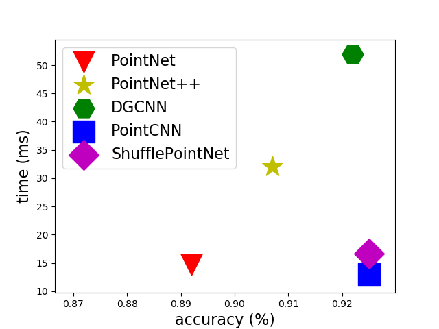
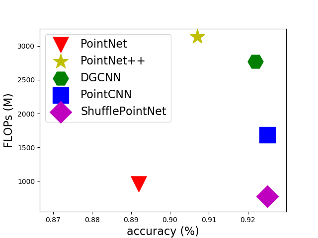
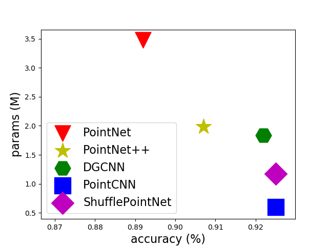
Figure 1: Measurement of accuracy, parameters, FLOPs and forward time. It shows that our proposed ShufflePointNet (magenta diamond marker) always stays on the lower right region, which represents the efficiency of our model in both accuracy and model complexity.

We notice that modern neural networks for point cloud [25, 27, 36, 8] heavily rely on dense Multi-Layer-Perceptron (MLP) to build repeated block structures with the different number of filters, but eliminating redundancy for dense MLP operation is rarely mentioned for point cloud analysis, although it is common in computer vision domain [38, 12, 29, 41, 40]. In point cloud domain, less redundancy brings more potential for some applications (e.g. autonomous driving) that need to process large scale point cloud. On one hand, the MLP operation is not spatial convolution, which limits the ability of local feature extraction. As a result, applying too many and deeper MLP convolutions easily leads to overfitting. On the other hand, MLP operation is efficient to deal with unstructured data (e.g. point cloud, social networks), as regular CNNs are only available on standard grid structure. Therefore, we draw attention to sparse MLP convolution over irregular point cloud, which can not only leverage advantages of MLP convolutions, but also reduce redundancy by making MLP convolution sparse.

Inspired by group convolution that is introduced by [16, 41] and can be treated as standard convolution with sparse filters, we primarily focus on building a deep-wide neural network to reduce complexity and also achieve high performance. The main contributions of this paper are summarized as follows:

• An efficient deep-wide neural network, named ShufflePointNet, is introduced, aimed at significantly reducing redundancy in depth and exploiting more feature information in width for point cloud understanding.

• We combine advantages of both MLP and group convolution to achieve better performance with less complexity for point cloud analysis.

• We propose to split features into groups, and to use the shuffle operation to exchange information between groups.

• We evaluate our model on extensive benchmarks, including small point cloud dataset (e.g. ModelNet40, ShapeNet part), large-scale point cloud (e.g. S3DIS) and super large-scale point cloud (KITTI), to represent efficiency over different scales data.

• To the best of our knowledge, ShufflePointNet is the first deep-wide model employing channel shuffle operation and group convolution to efficiently capture local representations for point cloud.

Figure 2: MLP Shuffled Group Convolution unit (SGC unit). We take the feature with $N\times K\times F$ as input, where $N,K,F$ indicate the number of points, neighbors and feature channels respectively. Assuming the dimension of output feature is $N\times K\times f$. For the standard MLP convolution, we apply $1\times 1$ convolution with $f$ filters to input feature, and the number of parameters is $F\times f$. For our SGC unit, the number of parameters is reduced to $\frac{F\times f}{g}$, where $g$ is the number of groups.

II Related work

Volumetric grid and multi-view methods.

Volumetric methods [23, 15, 4, 28] convert irregular point cloud to regular dense grid and voxels to allow feature extraction by standard CNNs. However, applying CNNs over dense volumetric grid leads to extremely high cost on computation and memory. [15, 28] improve efficiency in space partition and resolution, but still cause loss of local geometric information due to bounding voxels.

Multi-view methods [26, 32] apply classic 2D CNNs on group of 2D image views that are obtained from 3D objects by different angles. However, 3D geometric shape is unlikely to be captured from these 2D images due to lack of depth information. Besides, part of points information might be lost due to the occlusions on the images. As a result, it is non-trivial to segment every point for classification.

Deep learning methods directly on unstructured point cloud.

PointNet [25] takes the lead in treating point cloud as a set of unordered points and applying stacked Multi-Layer-Perceptron (MLP) to learn individual point feature. The global feature is finally obtained by a symmetric function (e.g. max pooling). However, local region features that are beneficial to better understanding geometric shape are not considered in this approach. In order to improve performance and remedy this drawback, PointNet++ [27] constructs a hierarchical neural network that recursively applies PointNet on local features that combine sampled points with corresponding neighboring points. DGCNN [36] applies PointNet on edge features that concatenate each point and its edges connecting corresponding point and its neighboring pairs. PointCNN [19] transforms a given irregular point cloud to a latent canonical order by learning a $\chi$-convolutional operator, after which classic 2D CNNs are available to use for local feature extraction. [20] attempts to learn a customized convolutional weight from geometric local relation for shape-aware representation.

Geometric deep learning methods.

Geometric deep learning [5] is defined as a modern term for deep neural network techniques that address non-Euclidean structured data (e.g. point cloud, social networks). Graph CNNs [7, 10, 42] have achieved great success in many tasks for graph representation of non-Euclidean data. Superpoint [18] organizes point set into geometric elements, after which a graph CNN structure is applied to exploit local features.

III Model architecture

In this section, we explain the architecture of our model resorting to two components: MLP Shuffled Group Convolution unit (SGC unit for short) as shown in Figure 2 and model architecture in Figure 3. We define $X=\left\{x_{i}\in\mathbb{R}^{F},i=1,2,\ldots,N\right\}$ as a raw point set and input for our model, where $F$ is the dimension of point representation, $N$ is the number of points, and $x_{i}$ is 3D geometric position of each point. Other observations,such as color, intensity, surface normal, can also be used to augment each point feature information.

III-A Local feature representation

Representing point cloud to graph structure with nodes and edges is an applicable method due to the fact that each node and corresponding edges on a graph can be naturally defined point cloud as each point feature and its neighborhood. As a result, converting point cloud to a graph and applying neural networks on the graph structure is efficient to learn embedding information for neighborhood of each node.

We then construct a directed graph $G=(V,E)$ for a point set, where $V\subseteq\ \mathbb{R}^{F}$ is node for each point, and $E$ indicates the corresponding edges to neighborhood. Assuming the input of point set is more or less uniform distribution, we choose $k$-nearest neighbor ($k$-NN) search to explore neighborhood of each point, as it can guarantee fixed number of neighbors. We define $N_{i}$ as a neighborhood set of each point $x_{i}$, then feature vector of directed edge is defined as ${e_{i}}_{j}=(x_{i},x_{i}-{x_{i}}_{j})$, where center point $x_{i}\in V$, neighboring point $x_{j}\in N_{i}$, and ${x_{i}}_{j}$ is $x_{j}$ to $x_{i}$.

III-B Model complexity metrics

In order to show efficiency of group convolution, we firstly introduce several metrics to measure model complexity, such as memory size, computational cost and forward time. Specifically, memory size is calculated by the total number of parameters for convolution kernels, the number of floatingpoint operations (FLOPs) indicates computational cost of neural networks, forward time represents forward propagation time of neural networks. FLOPs is a widely used but indirect metric, and it can approximate model complexity by counting part of operations in the neural networks, such as the number of multiply-adds operation. The forward time is normally used as direct metric to measure model speed. It is worth mentioning that FLOPs and forward time vary on the different experimental environment. Besides, forward time is a necessary metric to measure model speed, as FLOPs is not sufficient to indicate all the operations in the model and corresponding time consuming.

III-C Group convolution

AlexNet [16] first introduces group convolution for distributing the model over two GPUs. Its effectiveness is also well demonstrated by [38, 12, 29, 41, 40] in image domain. We study that group convolution has several representative advantages. Firstly, it can ease the training of deep neural networks by reducing redundancy; Secondly, it is an efficient method to increase the width of the neural networks that allows more feature channels which is beneficial to encoding more information on each group if we consider constrained complexity budget; Thirdly, it can be also treated as sparse convolution, as convolution kernels on each group are only responsible to part of entire feature channel. Last but not least, it can relieve overfitting to some extent.

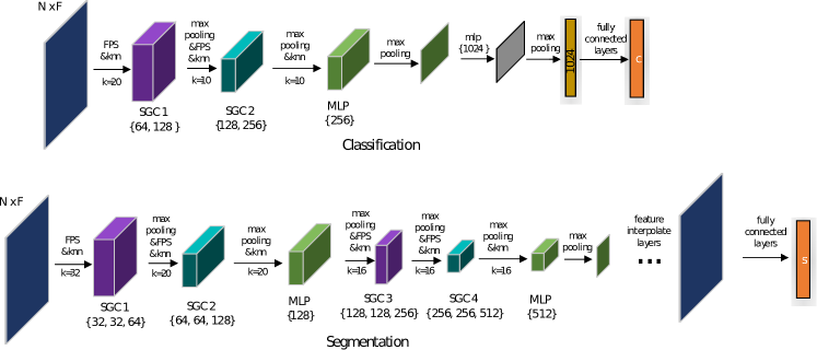
Figure 3: ShufflePointNet architecture: The architecture use PointNet++ as backbone, and it contains classification structure (top branch) and semantic segmentation structure (bottom branch) for point cloud. In detail, $N,F$ indicates the number of input points, and corresponding feature channels respectively. $k$ is the number of the neighbors. Besides, the number in the brace {} indicates the MLP filters.

The memory size and computational complexity (FLOPs) for a single $1\times 1$ group convolution can be calculated by Equations 1 and 2  [22] respectively. It is easy to observe that it becomes to standard MLP operation when we set $g=1$. Besides, the number of parameters and FLOPs are reduced to $1/g$ for a single operation when we split $k$-nn graph to $g$ groups.

$$params=1\times 1\times\frac{{C_{in}}}{g}\times\frac{{C_{out}}}{g}\times g=\frac{{C_{in}}\times{C_{out}}}{g}$$ (1)

$$FLOPs=\frac{N\times K\times{C_{in}}\times{C_{out}}}{g}$$ (2)

where ${C_{in}}$ and ${C_{out}}$ indicate input channel and output channel respectively, $N$ is the number of points, $K$ is the number of neighboring points, $g$ is the number of groups.

III-D Channel shuffle

Considering the fact that each group only holds incomplete and part representations of graph features, it is unlikely to capture sufficient features if there is no communication among multiple group convolutions. Inspired by [41], we stack group convolutions together and then shuffle the feature channel to sufficiently fuse features for all groups. We split fused features into $g$ groups again for the input of next layer as shown in Figure  2. As a result, each update group contains information of all other groups.

III-E Model architecture

Our ShufflePointNet architecture for shape classification and segmentation is shown in Figure  3. We use PointNet++ [27] as our backbone. However, there are three main differences between our model and PointNet++. Firstly, we use $1\times 1$ group convolutions to exploit local fine-grained features in both depth and width. Secondly, instead of radius search for neighboring points in PointNet++, we employ $k$-NN search to guarantee fixed number of neighbors. Thirdly, instead of neighboring point feature, edge feature connecting each point and corresponding neighbors is used to explicitly represent the relative position of neighboring point to its center point.

IV Experiments

In this section, we perform comprehensive experiments to evaluate our ShufflePointNet model in both shape classification and segmentation tasks. To demonstrate effectiveness of our model, we compare accuracy and complexity to recent state-of-the-art methods. We further arrange ablation study to carefully investigate different settings.

TABLE I: Semantic part segmentation results on ShapeNet part dataset.

	avg	air.	bag	cap	car	cha.	ear.	gui.	kni.	lam.	lap.	mot.	mug	pis.	roc.	ska.	tab.
kd-net [15]	82.3	82.3	74.6	74.3	70.3	88.6	73.5	90.2	87.2	81.0	94.9	57.4	86.7	78.1	51.8	69.9	80.3
Kc-Net [30]	83.7	82.8	81.5	86.4	77.6	90.3	76.8	91.0	87.2	84.5	95.5	69.2	94.4	81.6	60.1	75.2	81.3
PointNet [25]	83.7	83.4	78.7	82.5	74.9	89.6	73.0	91.5	85.9	80.8	95.3	65.2	93.0	81.2	57.9	72.8	80.6
3DmFV [3]	84.3	82.0	84.3	86.0	76.9	89.9	73.9	90.8	85.7	82.6	95.2	66.0	94.0	82.6	51.5	73.5	81.8
RSNet [13]	84.9	82.7	86.4	84.1	78.2	90.4	69.3	91.4	87.0	83.5	95.4	66.0	92.6	81.8	56.1	75.8	82.2
PointNet++ [27]	85.1	82.4	79.0	87.7	77.3	90.8	71.8	91.0	85.9	83.7	95.3	71.6	94.1	81.3	58.7	76.4	82.6
DGCNN [36]	85.1	84.2	83.7	84.4	77.1	90.9	78.5	91.5	87.3	82.9	96.0	67.8	93.3	82.6	59.7	75.5	82.0
SGPN	85.8	80.4	78.6	78.8	71.5	88.6	78.0	90.9	83.0	78.8	95.8	77.8	93.8	87.4	60.1	92.3	89.4
OURS	85.1	82.7	83.6	86.2	77.3	90.3	78.7	90.9	87.4	84.6	94.6	68.5	94.5	82.9	51.3	73.4	82.3

IV-A Classification

Dataset.

We evaluate our classification model on the ModelNet40 benchmark [37]. It contains 9,843 training models and 2,468 testing models that are classified to 40 classes. We firstly uniformly down sample all models to 1,024 points from total 2,048 points, and then normalize them into the unit sphere. Besides, in order to improve robustness, we further augment the training models by rotating, scaling the sampled points in random, and jittering the position of every point using Gaussian noise with zero mean and 0.01 standard deviation.

Training details.

Our model is implemented using TensorFlow v1.6. Adam optimizer [14] with batch size 32 is employed in the training. The learning rate is initially set to 0.001, and then decays with a rate of 0.7 every 20 epochs to 0.00001. The momentum for batch normalization starts from 0.9 and increases gradually with a decay rate of 0.5 every 20 epochs to 0.99.

Results.

Table II compares our shape classification model to recent state-of-the-art models for both accuracy and model complexity, including mean per-class accuracy (mA %), overall accuracy (OA %), the number of parameters (Million), FLOPs (Million) and forward time (ms) on the ModelNet40 benchmark [37]. Figure 1 also shows the efficiency of our model by illustrating that it stays at the lower right region all the time compared to other state-of-the-art models.

It is worth to mention that compared to backbone structure PointNet++ [27], our model outperforms by 1.8% for accuracy, and reduced the amount of parameters, FLOPs and forward time significantly by 41%, 75%, 48% respectively. Besides, compared to the complexity of single scale PointNet++ (params: 1.48M, FLOPs: 1684M, time: 20ms), our model still reduced parameters by 21%, FLOPs by 54% and forward time by 17%. The results convincingly verify the effectiveness of our deep-wide model.

We observe that PointCNN [19] has larger FLOPs but least forward time, while SpecGCN [33] has much similar FLOPs to PointNet but consumes much longer forward time. It proves our hypothesis that FLOPs is just indirect method to estimate model complexity, and it cannot be used alone to show the efficiency of model speed.

TABLE II: Classification results on ModelNet40 dataset.

methods	mA(%)	OA(%)	params	FLOPs	time
VoxNet [23]	83.0	85.9	-	-	-
PointNet [25]	86.0	89.2	3.48M	957M	14.7ms
PointNet++ [27]	-	90.7	1.99M	3136M	32.0ms
KC-Net [30]	-	91.0	-	-	-
SpecGCN [33]	-	91.5	2.05M	1112M	11254ms
KD-Net [15]	-	91.8	-	-	-
DGCNN [36]	90.2	92.2	1.84M	2768M	52.0ms
PCNN [2]	-	92.3	-	-	-
Ours	90.1	92.5	1.17M	770M	16.7ms
PointCNN [19]	88.8	92.5	0.6M	1682M	13.0ms
RS-CNN [20]	-	93.6	-	-	-

Ablation study.

We also test our classification model with different settings on the ModelNet40 benchmark [37].

Table III represents the performance for different number of groups. In order to evenly split feature channels, the initial input of SGC unit shares the same edge feature ${e_{i}}_{j}=(x_{i},x_{i}-{x_{i}}_{j})$ for all groups. It shows that the results for multiple groups ($g=2,4$) perform better than no grouping operation ($g=1$), as multiple groups help to capture more information for a given complexity budget. However, much larger group number (e.g. $g=8$ ) degenerates the performance. We discuss the reason that the useful feature information becomes limited for each group when we split feature channels to too many groups, which leads to the fact that the model is unlikely to learn useful information from individual group.

The number of parameters and FLOPs only have slightly drop, rather than half amount that is mentioned in Equation 1 and 2. The reason is that the fully-connected layers take up much large part of of complexity. However, it still shows effectiveness of group convolution, and our model manage to capture more useful information and reduced by 18.6% FLOPs compared to $g=1$.

The forward time also increases when the group number becomes larger, as more groups need more time to store corresponding features and parameters to the cache [22].

Table IV shows different settings for the number of points, low-level edge features ${e_{i}}_{j}$ and grouping methods. It indicates that there is no improvement when we add neighbor features to represent local features, and edge features connecting center point to corresponding neighborhood is beneficial to better results. Besides, $k$-NN searching slightly outperforms radius searching. We discuss that $k$-NN searching is more efficient when the layout of dataset can be more or less treated as uniform distribution.

TABLE III: Model complexity and accuracy for different groups

groups	OA (%)	params	FLOPs	time
$g=1$	91.8	1.20M	946M	15.3ms
$g=2$	92.5	1.17M	770M	16.7ms
$g=4$	92.3	1.15M	692M	19.5ms
$g=8$	91.5	1.14M	650M	22.7ms

TABLE IV: Ablation study of ShufflePointNet.

model	points	edge feature ${e_{i}}_{j}$	grouping	OA (%)
A	1k	$(x_{i},x_{i}-{x_{i}}_{j})$	knn	92.5
B	1k	$(x_{i},{x_{i}}_{j})$	knn	92.0
C	1k	$(x_{i},{x_{i}}_{j},x_{i}-{x_{i}}_{j})$	knn	92.5
D	2k	$(x_{i},x_{i}-{x_{i}}_{j})$	knn	92.7
E	1k	$(x_{i},x_{i}-{x_{i}}_{j})$	radius search	92.1

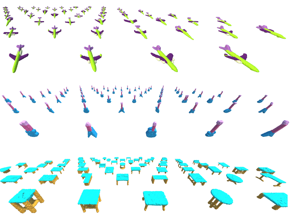
(a) Visualization

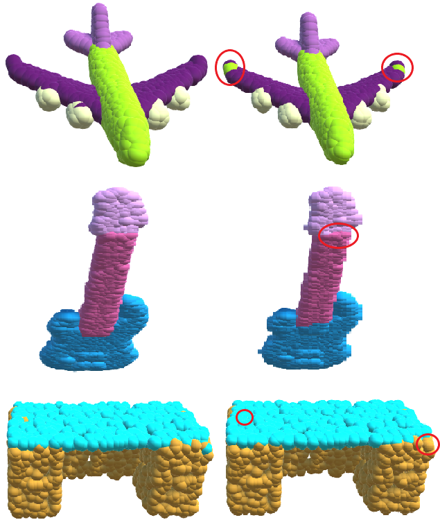
(b) Comparison

Figure 4: Visualization of semantic part segmentation results. Figure 4(a) visualizes some samples: airplane (top), guitar (middle), and table (bottom). While Figure 4(b) visualizes the predictions and corresponding errors (right) compared to ground truth (left).

TABLE V: Segmentation results on KITTI.

model	mIoU	accuracy	vehicle	cyclist	pedestrian	background
SegCloud [31]	36.8%	-	67.5	7.3%	53.5%	-
PointNet [25]	38.1%	92%	76.7%	2.9%	6.6%	89.8%
PCCN [35]	58.1%	95.5%	91.8%	40.2%	47.7%	89.3%
OURS	72.3%	96.8%	84.9%	54.0%	61.3%	95.5%

IV-B Semantic segmentation

We evaluate our segmentation model on ShapeNet part dataset [39], Stanford Large-Scale 3D Indoor Spaces Dataset (S3DIS) [1] and KITTI [11].

ShapeNet part dataset.

The dataset is composed of 16,881 CAD models (14,007 training models and 2,874 testing models ) that are classified to16 categories, and each model is annotated with several parts (less than 6) from 50 part classes. We follow the same sampling strategy as Section IV-A to sample 2,048 points uniformly. The task is to classify each point as part category from models.

S3DIS dataset.

S3DIS uses Matterport scanners to collect 6-dimension (XYZ, RGB) point clouds, which are then processed to 9D feature (XYZ, RGB, normalized spatial coordinate), from 271 rooms in 6 areas. We follow the settings in DGCNN [36] to slice all the rooms into 1m by 1m blocks, each of which are then sampled to 4,096 points during training process. Meanwhile, we use all points to evaluate our model. We test our model on area 5, and training process is applied on other areas.

KITTI dataset.

We use KITTI Object Detection Benchmark [11] to evaluate our model on real traffic scene. We follow [9] to separate the KITTI dataset to 7,481 for training and 191 for testing. However, due to the fact that each frame contains approximate 100,000 points, it is infeasible to apply all points on our model. Therefore, we firstly downsample points from about 100k to 16k (16384 points) by the strategy that we remove points that outside image view, then we randomly select 11,469 points (70%) in 40 meters and 4915 points for the rest.

Training details.

We follow all the training settings in classification task, except that batch size is set to 24, and we distribute the task to two NVIDIA TESLA V100 GPUs.

Results.

The mean Intersection over Union (mIoU) [25] is used to evaluate segmentation performance. The IoU is calculated by averaging IoUs for all parts belonging to the same categories, then the mIoU is the mean IoUs for all shapes from testing dataset.

For the semantic part segmentation task, Table I indicates that our segmentation model achieves competitive results on the ShapeNet part dataset [39]. It wins 4 categories that is the same amount as DGCNN and SGPN. We also illustrate some shapes from our results in Figure 4(a), and visualize the errors of our prediction results compared to ground truth as shown in Figure 4(b) . We represent the ground truth on the left and our predictions and errors on the right.

Table VI and  V indicate that our segmentation model achieves competitive result on S3DIS and wins the best performance on KITTI dataset. We also observe that both our model and PointNet++ (reproduced) perform worse for mIoU results, even if the overall accuracy is competitive. We discuss the reason that compared to other models, our model and PointNet++ are likely to lose feature information to some extent when apply downsampling and feature interpolation for upsampling layers, although it leads to less model complexity.

TABLE VI: Segmentation results on S3DIS Area 5.

model	mIoU	overall accuracy
SegCloud [31]	48.9%	-
PointNet [25]	47.6%	78.5%
PointNet++ [27] (Repro)	48.3%	84.0%
DGCNN [36]	56.1%	84.1%
OURS	50.7%	84.3%
PointCNN [19]	57.3%	85.9%
SPGraph [18]	58.0%	86.4%

V Conclusions

In this paper, we propose a deep-wide neural network, named ShufflePointNet, to exploit local representations in both depth and width for point cloud. The success of our model verifies that deep-wide neural network can achieve high performance with less model complexity. In the future, we consider to apply our model on the real applications, such as environment perception for our autonomous vehicle that needs to process very large-scale point cloud data.

References

- [1] Iro Armeni, Ozan Sener, Amir R Zamir, Helen Jiang, Ioannis Brilakis, Martin Fischer, and Silvio Savarese. 3d semantic parsing of large-scale indoor spaces. In Proceedings of the IEEE Conference on Computer Vision and Pattern Recognition, pages 1534–1543, 2016.
- [2] Matan Atzmon, Haggai Maron, and Yaron Lipman. Point convolutional neural networks by extension operators. arXiv preprint arXiv:1803.10091, 2018.
- [3] Yizhak Ben-Shabat, Michael Lindenbaum, and Anath Fischer. 3d point cloud classification and segmentation using 3d modified fisher vector representation for convolutional neural networks. arXiv preprint arXiv:1711.08241, 2017.
- [4] Jon Louis Bentley. Multidimensional binary search trees used for associative searching. Communications of the ACM, 18(9):509–517, 1975.
- [5] Michael M Bronstein, Joan Bruna, Yann LeCun, Arthur Szlam, and Pierre Vandergheynst. Geometric deep learning: going beyond euclidean data. IEEE Signal Processing Magazine, 34(4):18–42, 2017.
- [6] Gerd Bruder, Frank Steinicke, and Andreas Nüchter. Poster: Immersive point cloud virtual environments. In 2014 IEEE Symposium on 3D User Interfaces (3DUI), pages 161–162. IEEE, 2014.
- [7] Joan Bruna, Wojciech Zaremba, Arthur Szlam, and Yann LeCun. Spectral networks and locally connected networks on graphs. arXiv preprint arXiv:1312.6203, 2013.
- [8] Can Chen, Luca Zanotti Fragonara, and Antonios Tsourdos. Gapnet: Graph attention based point neural network for exploiting local feature of point cloud. arXiv preprint arXiv:1905.08705, 2019.
- [9] Xiaozhi Chen, Huimin Ma, Ji Wan, Bo Li, and Tian Xia. Multi-view 3d object detection network for autonomous driving. In Proceedings of the IEEE Conference on Computer Vision and Pattern Recognition, pages 1907–1915, 2017.
- [10] Michaël Defferrard, Xavier Bresson, and Pierre Vandergheynst. Convolutional neural networks on graphs with fast localized spectral filtering. In Advances in neural information processing systems, pages 3844–3852, 2016.
- [11] Andreas Geiger, Philip Lenz, Christoph Stiller, and Raquel Urtasun. Vision meets robotics: The kitti dataset. The International Journal of Robotics Research, 32(11):1231–1237, 2013.
- [12] Andrew G Howard, Menglong Zhu, Bo Chen, Dmitry Kalenichenko, Weijun Wang, Tobias Weyand, Marco Andreetto, and Hartwig Adam. Mobilenets: Efficient convolutional neural networks for mobile vision applications. arXiv preprint arXiv:1704.04861, 2017.
- [13] Qiangui Huang, Weiyue Wang, and Ulrich Neumann. Recurrent slice networks for 3d segmentation of point clouds. In Proceedings of the IEEE Conference on Computer Vision and Pattern Recognition, pages 2626–2635, 2018.
- [14] Diederik P Kingma and Jimmy Ba. Adam: A method for stochastic optimization. arXiv preprint arXiv:1412.6980, 2014.
- [15] Roman Klokov and Victor Lempitsky. Escape from cells: Deep kd-networks for the recognition of 3d point cloud models. In Proceedings of the IEEE International Conference on Computer Vision, pages 863–872, 2017.
- [16] Alex Krizhevsky, Ilya Sutskever, and Geoffrey E Hinton. Imagenet classification with deep convolutional neural networks. In Advances in neural information processing systems, pages 1097–1105, 2012.
- [17] Jason Ku, Melissa Mozifian, Jungwook Lee, Ali Harakeh, and Steven L Waslander. Joint 3d proposal generation and object detection from view aggregation. In 2018 IEEE/RSJ International Conference on Intelligent Robots and Systems (IROS), pages 1–8. IEEE, 2018.
- [18] Loic Landrieu and Martin Simonovsky. Large-scale point cloud semantic segmentation with superpoint graphs. In Proceedings of the IEEE Conference on Computer Vision and Pattern Recognition, pages 4558–4567, 2018.
- [19] Yangyan Li, Rui Bu, Mingchao Sun, Wei Wu, Xinhan Di, and Baoquan Chen. Pointcnn: Convolution on x-transformed points. In Advances in Neural Information Processing Systems, pages 828–838, 2018.
- [20] Yongcheng Liu, Bin Fan, Shiming Xiang, and Chunhong Pan. Relation-shape convolutional neural network for point cloud analysis. In Proceedings of the IEEE Conference on Computer Vision and Pattern Recognition, pages 8895–8904, 2019.
- [21] Zhongze Liu, Huiyan Chen, Huijun Di, Yi Tao, Jianwei Gong, Guangming Xiong, and Jianyong Qi. Real-time 6d lidar slam in large scale natural terrains for ugv. In 2018 IEEE Intelligent Vehicles Symposium (IV), pages 662–667. IEEE, 2018.
- [22] Ningning Ma, Xiangyu Zhang, Hai-Tao Zheng, and Jian Sun. Shufflenet v2: Practical guidelines for efficient cnn architecture design. In Proceedings of the European Conference on Computer Vision (ECCV), pages 116–131, 2018.
- [23] Daniel Maturana and Sebastian Scherer. Voxnet: A 3d convolutional neural network for real-time object recognition. In 2015 IEEE/RSJ International Conference on Intelligent Robots and Systems (IROS), pages 922–928. IEEE, 2015.
- [24] Charles R Qi, Wei Liu, Chenxia Wu, Hao Su, and Leonidas J Guibas. Frustum pointnets for 3d object detection from rgb-d data. In Proceedings of the IEEE Conference on Computer Vision and Pattern Recognition, pages 918–927, 2018.
- [25] Charles R Qi, Hao Su, Kaichun Mo, and Leonidas J Guibas. Pointnet: Deep learning on point sets for 3d classification and segmentation. Proc. Computer Vision and Pattern Recognition (CVPR), IEEE, 1(2):4, 2017.
- [26] Charles R Qi, Hao Su, Matthias Nießner, Angela Dai, Mengyuan Yan, and Leonidas J Guibas. Volumetric and multi-view cnns for object classification on 3d data. In Proceedings of the IEEE conference on computer vision and pattern recognition, pages 5648–5656, 2016.
- [27] Charles Ruizhongtai Qi, Li Yi, Hao Su, and Leonidas J Guibas. Pointnet++: Deep hierarchical feature learning on point sets in a metric space. In Advances in Neural Information Processing Systems, pages 5099–5108, 2017.
- [28] Gernot Riegler, Ali Osman Ulusoy, and Andreas Geiger. Octnet: Learning deep 3d representations at high resolutions. In Proceedings of the IEEE Conference on Computer Vision and Pattern Recognition, pages 3577–3586, 2017.
- [29] Mark Sandler, Andrew Howard, Menglong Zhu, Andrey Zhmoginov, and Liang-Chieh Chen. Mobilenetv2: Inverted residuals and linear bottlenecks. In Proceedings of the IEEE Conference on Computer Vision and Pattern Recognition, pages 4510–4520, 2018.
- [30] Yiru Shen, Chen Feng, Yaoqing Yang, and Dong Tian. Mining point cloud local structures by kernel correlation and graph pooling. In Proceedings of the IEEE conference on computer vision and pattern recognition, pages 4548–4557, 2018.
- [31] Lyne Tchapmi, Christopher Choy, Iro Armeni, JunYoung Gwak, and Silvio Savarese. Segcloud: Semantic segmentation of 3d point clouds. In 2017 International Conference on 3D Vision (3DV), pages 537–547. IEEE, 2017.
- [32] Chu Wang, Marcello Pelillo, and Kaleem Siddiqi. Dominant set clustering and pooling for multi-view 3d object recognition. In Proceedings of British Machine Vision Conference (BMVC), volume 12, 2017.
- [33] Chu Wang, Babak Samari, and Kaleem Siddiqi. Local spectral graph convolution for point set feature learning. In Proceedings of the European Conference on Computer Vision (ECCV), pages 52–66, 2018.
- [34] Dominic Zeng Wang and Ingmar Posner. Voting for voting in online point cloud object detection. In Robotics: Science and Systems, volume 1, pages 10–15607, 2015.
- [35] Shenlong Wang, Simon Suo, Wei-Chiu Ma, Andrei Pokrovsky, and Raquel Urtasun. Deep parametric continuous convolutional neural networks. In Proceedings of the IEEE Conference on Computer Vision and Pattern Recognition, pages 2589–2597, 2018.
- [36] Yue Wang, Yongbin Sun, Ziwei Liu, Sanjay E Sarma, Michael M Bronstein, and Justin M Solomon. Dynamic graph cnn for learning on point clouds. arXiv preprint arXiv:1801.07829, 2018.
- [37] Zhirong Wu, Shuran Song, Aditya Khosla, Fisher Yu, Linguang Zhang, Xiaoou Tang, and Jianxiong Xiao. 3d shapenets: A deep representation for volumetric shapes. In Proceedings of the IEEE conference on computer vision and pattern recognition, pages 1912–1920, 2015.
- [38] Saining Xie, Ross Girshick, Piotr Dollár, Zhuowen Tu, and Kaiming He. Aggregated residual transformations for deep neural networks. In Proceedings of the IEEE conference on computer vision and pattern recognition, pages 1492–1500, 2017.
- [39] Li Yi, Vladimir G Kim, Duygu Ceylan, I Shen, Mengyan Yan, Hao Su, Cewu Lu, Qixing Huang, Alla Sheffer, Leonidas Guibas, et al. A scalable active framework for region annotation in 3d shape collections. ACM Transactions on Graphics (TOG), 35(6):210, 2016.
- [40] Ting Zhang, Guo-Jun Qi, Bin Xiao, and Jingdong Wang. Interleaved group convolutions. In Proceedings of the IEEE International Conference on Computer Vision, pages 4373–4382, 2017.
- [41] Xiangyu Zhang, Xinyu Zhou, Mengxiao Lin, and Jian Sun. Shufflenet: An extremely efficient convolutional neural network for mobile devices. In Proceedings of the IEEE Conference on Computer Vision and Pattern Recognition, pages 6848–6856, 2018.
- [42] Yingxue Zhang and Michael Rabbat. A graph-cnn for 3d point cloud classification. In 2018 IEEE International Conference on Acoustics, Speech and Signal Processing (ICASSP), pages 6279–6283. IEEE, 2018.
- [43] Yingxue Zhang and Michael Rabbat. A graph-cnn for 3d point cloud classification. In International Conference on Acoustics, Speech and Signal Processing (ICASSP), Calgary, Canada, 2018.
- [44] Yin Zhou and Oncel Tuzel. Voxelnet: End-to-end learning for point cloud based 3d object detection. In Proceedings of the IEEE Conference on Computer Vision and Pattern Recognition, pages 4490–4499, 2018.