The ASKAP-EMU Early Science Project:
Radio Continuum Survey of the Small Magellanic Cloud

Abstract

We present two new radio continuum images from the Australian Square Kilometre Array Pathfinder (ASKAP) survey in the direction of the Small Magellanic Cloud (SMC). These images are part of the Evolutionary Map of the Universe (EMU) Early Science Project (ESP) survey of the Small and Large Magellanic Clouds. The two new source lists produced from these images contain radio continuum sources observed at 960 MHz (4489 sources) and 1320 MHz (5954 sources) with a bandwidth of 192 MHz and beam sizes of 30.0″$\times$30.0″ and 16.3″$\times$15.1″, respectively. The median Root Mean Squared (RMS) noise values are 186 $\mu$Jy beam^-1 (960 MHz) and 165 $\mu$Jy beam^-1 (1320 MHz). To create point source catalogues, we use these two source lists, together with the previously published Molonglo Observatory Synthesis Telescope (MOST) and the Australia Telescope Compact Array (ATCA) point source catalogues to estimate spectral indices for the whole population of radio point sources found in the survey region. Combining our ASKAP catalogues with these radio continuum surveys, we found 7736 point-like sources in common over an area of 30 deg². In addition, we report the detection of two new, low surface brightness supernova remnant candidates in the SMC. The high sensitivity of the new ASKAP ESP survey also enabled us to detect the bright end of the SMC planetary nebula sample, with 22 out of 102 optically known planetary nebulae showing point-like radio continuum emission. Lastly, we present several morphologically interesting background radio galaxies.

1 Introduction

This is an exciting time for the study of nearby galaxies. These nearby external galaxies offer an ideal laboratory, since they are close enough to be resolved, yet located at relatively well known distances (see e.g. Pietrzyński et al., 2019). New generations of Magellanic Cloud (MC) surveys across the entire electromagnetic spectrum reflect a major opportunity to study different objects and processes in the elemental enrichment of the Interstellar Medium (ISM). The study of these interactions in different domains, including radio, optical and X-ray, allow a better understanding of objects such as supernova remnants (SNRs), planetary nebulae (PNe), (Super)Bubbles and their environments, young stellar objects (YSOs), symbiotic (accreting compact object) binaries and Wolf-Rayet (WR) wind-wind-collision binaries.

Various new high resolution ($\sim$1″) and high sensitivity surveys of the Small and Large Magellanic Clouds (MCs), such as XMM–Newton and Chandra (X-rays; see e.g. Haberl et al., 2012b), Herschel (Gordon et al., 2011) and Spitzer (IR; Meixner et al., 2006), UM/CTIO Magellanic Cloud Emission Line Survey (MCELS, optical; Winkler et al., 2005) and ATCA/MOST (radio), provide a solid base for detailed multi-wavelength studies of radio objects within and behind the MCs.

Our main area of interest is the radio objects natal to the MCs, particularly SNRs and PNe. To date, some 85 SNRs in the MCs have been identified, with a further 20 candidates awaiting confirmation (Maggi et al., 2016; Bozzetto et al., 2017). Similarly, over 50 PNe (Filipović et al., 2009; Bojičić et al., 2010; Leverenz et al., 2016; Leverenz et al., 2017) and hundreds of H ii regions and YSOs have been identified (see for example Oliveira et al., 2013). Over 8500 radio sources have also been detected in the region of the Clouds – mainly AGN, radio galaxies and quasars (Wong et al., 2012b; Collier, 2016, Grieve et al. in prep.). Additionally, some comprehensive studies of the magnetic fields of the MCs have been undertaken with the present generation of radio continuum surveys (ATCA; Gaensler et al., 2005; Mao et al., 2008, 2012).

In this paper, we focus on the Small Magellanic Cloud (SMC), a dwarf irregular galaxy. Its proximity ($\sim$60 kpc; Hilditch et al., 2005) enables us to conduct detailed radio frequency studies of its gas and stellar content, without the complication of the foreground emission and absorption we encounter when working within our own Galaxy. For these reasons, the SMC has been the subject of many radio studies over several decades.

Starting in the mid 1970s, the SMC has been the subject of both single dish and interferometric radio continuum surveys. These monitoring campaigns have produced over a dozen catalogues of sources towards the SMC (Clarke, 1976; McGee et al., 1976; Haynes et al., 1986; Wright & Otrupcek, 1990; Filipović et al., 1997; Turtle et al., 1998; Filipović et al., 1998; Filipović et al., 1997, 2002; Payne et al., 2004; Filipović et al., 2005; Reid et al., 2006; Payne et al., 2007; Wong et al., 2011a; Crawford et al., 2011; Wong et al., 2011b, 2012a, 2012b; For et al., 2018) (see also Table 1 in Wong et al., 2011b, for details).

For the reasons mentioned above, the SMC was also selected as a prime target for the Early Science Project (ESP) of the newly built Australian Square Kilometre Array Pathfinder (ASKAP; Johnston et al., 2008). ASKAP is a radio interferometer that allows us to survey the SMC with regularly sampled observations. ASKAP also provides sensitivity down to the $\mu$Jy range as well as a large field of view of 30 deg² (Murphy et al., 2013). The goal of this project is to produce high sensitivity and high resolution continuum images of the MCs as well as to catalogue discrete radio continuum sources.

The ASKAP EMU ESP survey will be a good complement to and, in some cases, a significant improvement on previous similar studies of the southern skies. For instance, the Australia Telescope Large Area Survey (ATLAS; Norris et al., 2006; Middelberg et al., 2008) was a 1400 MHz radio survey covering a total of roughly 6 deg² on the sky, down to an RMS noise level of $<$30 $\mu$Jy, requiring 380 hours of observation time. This survey uncovered over 3000 distinct radio sources out to a redshift of 2. ASKAP’s higher resolution and increased sensitivity will be able to achieve such results on a much shorter time scale (see Fig. 1 in Franzen et al., 2015).

Another obvious advantage of ASKAP is the size of the field of view. For example, the Sydney University Molonglo Sky Survey (SUMSS) would need $\sim$16 fields and $\sim$192 hours to cover the ASKAP EMU SMC survey area to the required sensitivity (see Mauch et al., 2003); in contrast the ASKAP observations were composed of eight fields of about 12 hours each (a total of 96 hours).

In this paper we present two new catalogues from the ASKAP ESP surveys for different types of radio continuum sources towards the SMC. These catalogues were obtained from images taken at 960 MHz ($\lambda=32$ cm) and 1320 MHz ($\lambda=23$ cm). For the point source catalogue, we combine the ASKAP data with the previously published MOST catalogue (Turtle et al., 1998; Wong et al., 2011b) and the ATCA $\lambda$= 20, 13, 6 and 3 cm catalogues (Wong et al., 2011b, 2012a, and references therein).

The paper is laid out as follows: Section 2 describes the data used to create the source lists. In section 3.1 we describe the source detection methods used, section 3.2 describes the new ASKAP source catalogues and in section 3.3 we compare our work to previous catalogues of point sources towards the SMC. Sections 4 and 5 describe the latest ASKAP SMC populations of SNRs and PNe, respectively. In Section 6, we briefly discuss other sources of interest, including those behind the SMC.

2 Data, Observing and Processing

The SMC was observed as part of the ASKAP commissioning and early science verification (DeBoer et al., 2009; Hotan et al., 2014; McConnell et al., 2016). Here, we present observations at 960 MHz taken on 2017 September 3 (Figure 1; using 12 antennas: 2, 3, 4, 6, 12, 14, 16, 17, 19, 27, 28, and 30), and at 1320 MHz on 2017 November 3 - 5 (Figure 2, using 16 antennas: 1, 2, 3, 4, 5, 6, 10, 12, 14, 16, 17, 19, 24, 27, 28, 30). The H i spectral and dynamical analyses of the 1320 MHz data have been presented in McClure-Griffiths et al. (2018) and Di Teodoro et al. (2019) respectively.

We note that the current observations were made with only 33 per cent and 44 per cent (for 960 MHz and 1320 MHz respectively) of the full ASKAP antenna configuration and 66 per cent of the final bandwidth that will be available in the final array. We believe that with the full array, we will be able to achieve a factor of two increase in sensitivity compared to what is currently possible.

A bandwidth of 192 MHz was used and the maximum baseline for these observations was 2.3 km. The observations cover a total field of view of 30 deg², with exposure times of 10 to 11 hours per pointing. To optimise sensitivity and survey speed, the 36 beams on each antenna were configured in a hexagonal grid on the sky (McConnell, 2017). The source 1934-638 was observed and used for the flux density calibration of all images.

The data calibration, processing, and imaging were carried out using the ASKAPsoft pipeline (Cornwell et al., 2011). For both sets of images we processed the data with the multiscale clean algorithm, noting from our previous work (Wong et al., 2011a) that the largest detectable features were $\sim$192″. Therefore, we selected spacial scales of 192″, 96″ and 48″ as a geometric progression. We also noted features on the scale of 16″, and so this spatial scale was also selected. The 1320 MHz image was cleaned and then mosaiced. For the 960 MHz image, we set the pixel size to 6″, and set the restoring beam to $30\arcsec\times 30\arcsec$ in order to maximise our resolution and sensitivity and to more easily compare these new results with other SMC surveys referenced in this work.

The properties of the 960 MHz and 1320 MHz images are summarised in Table 1. These two new ASKAP images are shown in Figures 1 and 2, with zoomed in views showing the resolved structure of the emission in Figures. 3 and 4. Figures 5 and 6 show the RMS maps generated by the source finding software, aegean (Hancock et al., 2012, 2018) for the 960 MHz and 1320 MHz images respectively.

We note that our ESP 960 MHz image was made at very early stages of the ASKAP testing and a range of issues, such as positional accuracy and calibration, were discovered. We have made every effort to identify and correct these problems. The 1320 MHz image as made at a later date when these issues were already known and could therefore be avoided, mitigated or corrected as needed.

Table 1: Properties of the 960 MHz and 1320 MHz radio continuum images as well other MOST/ATCA surveys used in this study.

$\nu$	$\lambda$	Telescope	Median RMS	Best RMS	Beam Size	Total number	Reference
(MHz)	(cm)		($\mu$Jy beam-1)	($\mu$Jy beam-1)	(arcsec)	of point sources
1320	23	ASKAP	165	55	16.3 $\times$ 15.1	5954	This work
960	32	ASKAP	186	110	30.0 $\times$ 30.0	4489	This work
843	36	MOST	700	500	40.0 $\times$ 40.0	1689	Wong et al. (2011b)
1400	20	ATCA	700	600	17.8 $\times$ 12.2	1560	Wong et al. (2011b)
2370	13	ATCA	400	300	45.0 $\times$ 45.0	742	Wong et al. (2011b)
4800	6	ATCA	700	500	30.0 $\times$ 30.0	601	Wong et al. (2012a)
8640	3	ATCA	800	700	20.0 $\times$ 20.0	457	Wong et al. (2012a)

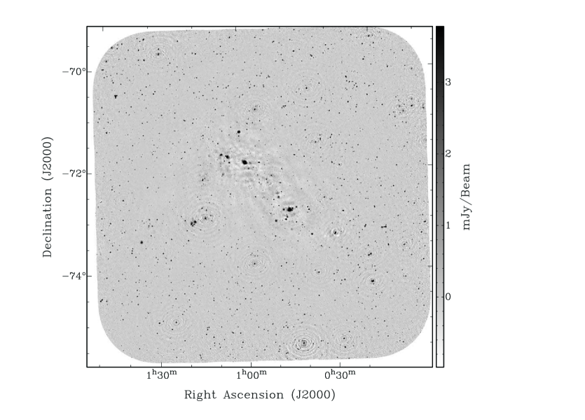
Figure 1: ASKAP ESP image of the SMC at 960 MHz. The beam size is 30.0″ $\times$ 30.0″ and the side scale bar represents the image grey scale intensity range.

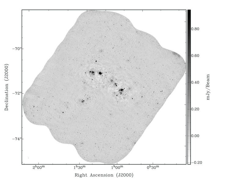
Figure 2: ASKAP ESP image of the SMC at 1320 MHz. The beam size is 16.3″ $\times$ 15.1″ and the side scale bar represents the image grey scale intensity range.

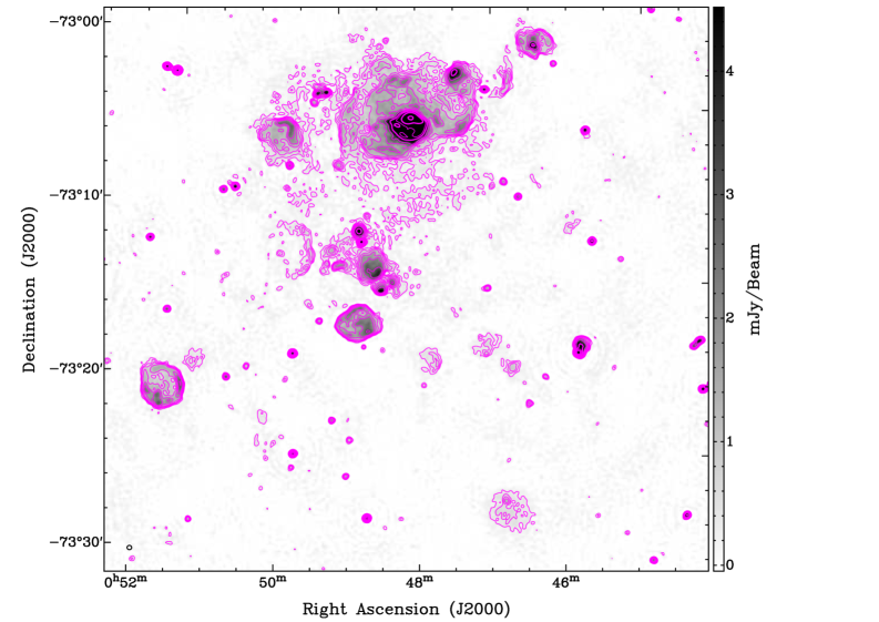
Figure 3: ASKAP ESP image of the SMC N 19 region at 1320 MHz (grey scale and contours). Magenta contours are: 0.3, 0.5, 0.7, 1, 1.5, 2, 3, 5, 7, 10 and 15 mJy beam^-1. The beam size of 16.3″ $\times$ 15.1″ is shown as a small black ellipse in the lower left corner.

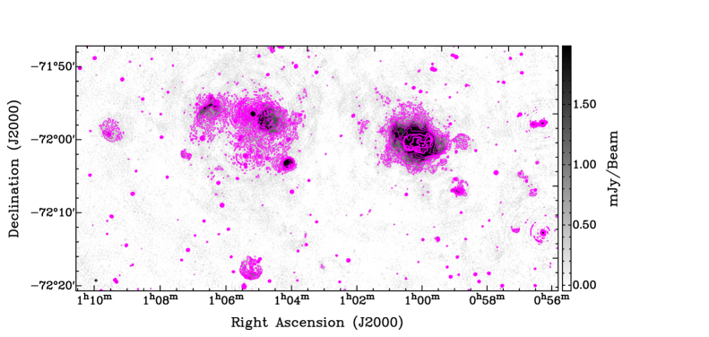
Figure 4: ASKAP ESP image of the SMC N 66 and SNR 1E0102-72 region at 1320 MHz (grey scale and contours). Magenta contours are: 0.3, 0.5, 0.7, 1, 1.5, 2, 3, 5, 7, 10 and 15 mJy beam^-1. The beam size of 16.3″ $\times$ 15.1″ is shown as a small black ellipse in the lower left corner.

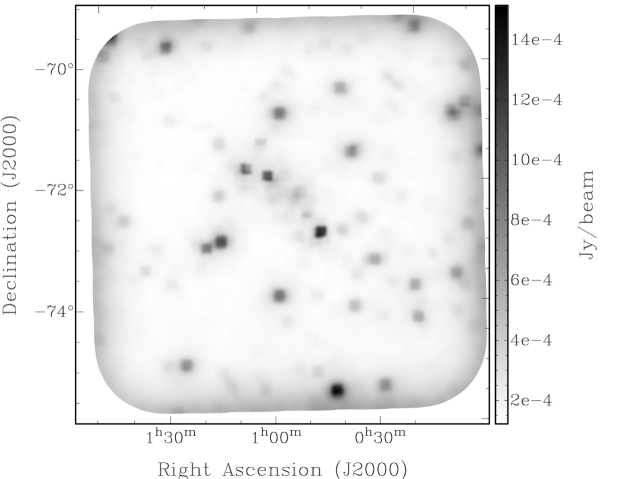
Figure 5: RMS map of the 960 MHz ASKAP observations, produced by BANE with the default parameters. The image is of the same pixel scale as in Figure 1. Higher RMS levels are found at the edge of the field (where only one beam is present) and around the brighter sources.

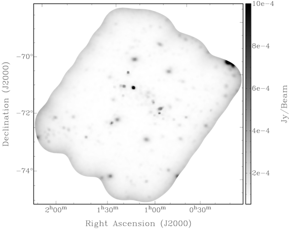
Figure 6: RMS map of the 1320 MHz ASKAP observations, produced by BANE with the default parameters. The image is of the same pixel scale as in Figure 2. Higher RMS levels are found at the edge of the field (where only one beam is present) and around the brighter sources.

3 ASKAP ESP SMC Source catalogues

3.1 Source detection

The aegean source finding software was used to create an overall catalogue of sources from the ASKAP images. Due to the combination of the multiple beams and artefacts from bright sources, images from ASKAP have variable noise across the field. This variable noise must be parameterised before source-finding to ensure that accurate source thresholds are determined. To do this, noise (RMS) and background level maps were made using the BANE routine in aegean, with its default parameters. BANE uses a grid algorithm with a sliding box-car and sigma-clipping approach, with the resulting maps being at the same pixel scale as the input images (for further detail, see Hancock et al., 2018). The maps were then used with the default parameters in aegean to create the initial source lists at 5$\sigma$ level. Visual inspection of the sources was carried out to verify detections from the initial source lists.

3.2 Source Catalogues

In total, we found 4489 and 5954 point sources in our new ASKAP 960 MHz and 1320 MHz images, respectively (see Tables 2 and 3). There are 3536 unique sources that have both ASKAP 960 MHz and 1320 MHz flux densities. This catalogue excludes known SMC SNRs, PNe and H ii regions which are listed separately (see Sections 4 and 5).

We combine our two new ASKAP catalogues of point sources with previously published source lists from MOST (at 843 MHz) and ATCA (1400, 2370, 4800 and 8640 MHz). To do this, we used a 10″ search radius to find common sources and found a total of 7736 discrete sources which we list in Table 4. Out of these 7736 sources, there are 659 sources that do not have any ASKAP flux densities and 112 that do not have MOST/SUMSS flux densities.

Where possible, we also list the estimated spectral index ($\alpha$) of the source including error (Table 4; Col. 12). We also note that there are 49 ($\sim$0.5 per cent of the total population) sources in Table 4 with questionable $\alpha$ estimates of $\alpha<-4$ and $\alpha>+2.5$. Where the $\alpha$ values are extreme we flag those sources to emphasis caution. The reasons behind such unrealistic $\alpha$ for these few sources ($<$0.3 per cent out of our 7736 sources) are twofold. One is that the flux density measurements are made between only two nearby frequency bands (such as for example 1400/1320 MHz or 960/843 MHz) where a small change (or error) in size or flux density leads to large changes and unrealistic estimates in $\alpha$. The second issue is that almost all of such sources lie near near the edges of the field where $uv$ coverage and sensitivity are significantly poorer.

Table 2: Point source catalogue derived from our ASKAP 960 MHz image. The catalogue at 960 MHz consists of 4489 point sources. The full table is available in the online version of the article.

Source	Name	RA (J2000)	Dec (J2000)	S960MHz
No.	ASKAP	hh mm ss	∘ ′ ″	(mJy)
1	J000437–744211	00:04:36.52	–74:42:11.0	4.0$\pm$0.5
2	J000506–751559	00:05:05.77	–75:15:58.6	4.0$\pm$0.5
3	J000508–745454	00:05:07.97	–74:54:53.6	16.0$\pm$0.5
4	J000545–741232	00:05:44.94	–74:12:31.6	16.9$\pm$0.6
5	J000550–744806	00:05:49.77	–74:48:05.9	27.7$\pm$0.5
6	J000550–742134	00:05:50.46	–74:21:34.4	3.6$\pm$0.5
7	J000603–743754	00:06:03.48	–74:37:54.1	10.9$\pm$0.5
8	J000608–740148	00:06:08.34	–74:01:47.6	8.2$\pm$0.6
9	J000608–740240	00:06:08.50	–74:02:40.2	9.4$\pm$0.6
10	J000609–740538	00:06:09.42	–74:05:38.3	2.9$\pm$0.6

Table 3: Point source catalogue derived from our ASKAP 1320 MHz image. The catalogue at 1320 MHz consists of 5954 point sources. The full table is available in the online version of the article.

Source	Name	RA (J2000)	Dec (J2000)	S1320MHz
No.	ASKAP	hh mm ss	∘ ′ ″	(mJy)
1	J000537–715839	00:05:36.81	–71:58:39.2	5.3$\pm$0.9
2	J000547–722502	00:05:46.55	–72:25:01.9	3.8$\pm$0.5
3	J000646–720801	00:06:45.91	–72:08:01.2	2.1$\pm$0.3
4	J000648–722252	00:06:48.25	–72:22:51.8	10.1$\pm$0.3
5	J000653–715740	00:06:52.59	–71:57:40.2	36.3$\pm$0.4
6	J000654–722034	00:06:54.07	–72:20:34.2	2.1$\pm$0.4
7	J000713–714611	00:07:12.94	–71:46:10.6	4.1$\pm$0.6
8	J000726–720631	00:07:26.15	–72:06:30.8	3.4$\pm$0.2
9	J000732–720732	00:07:31.97	–72:07:32.2	1.4$\pm$0.2
10	J000739–721026	00:07:38.64	–72:10:26.1	2.1$\pm$0.4

Table 4: An excerpt from the combined catalogue of point sources. These sources should be referred to as EMU-ESP-SMC-ffff NNNN. The full table is available in the online version of the article

. (1) (2) (3) (4) (5) (6) (7) (8) (9) (10) (11) (12) (13) (14) (15) No RA (J2000) DEC (J2000) S${}_{843\,\rm{MHz}}$ S${}_{960\,\rm{MHz}}$ S${}_{1320\,\rm{MHz}}$ S${}_{1400\,\rm{MHz}}$ S${}_{2370\,\rm{MHz}}$ S${}_{4800\,\rm{MHz}}$ S${}_{8640\,\rm{MHz}}$ No. $\alpha\pm\Delta\alpha$ S${}_{1\,\rm{GHz}}$ Cat. No. Cat. No. hh:mm:ss.s dd:mm:ss.s (mJy) (mJy) (mJy) (mJy) (mJy) (mJy) (mJy) points (mJy) 960 1320 3165 00:51:40.16 –72:38:16.5 6.19 5.5 4.1 … … … … 3 –0.94 $\pm$ 0.01 5.3 2021 2276 3166 00:51:41.38 –73:13:36.9 13.96 10.0 … 10.6 19.5 10.0 11.10 6 –0.10 $\pm$ 0.10 12.4 2022 … 3167 00:51:41.65 –70:28:46.3 … 1.1 0.82 … … … … 2 –0.92 1.1 2025 2278 3168 00:51:41.85 –69:45:10.2 … 3.5 2.7 … … … … 2 –0.81 3.4 2024 2279 3169 00:51:42.02 –72:55:56.3 71.88 61.3 … 38.42 42.6 21.3 7.26 6 –0.90 $\pm$ 0.10 61.7 2023 … 3170 00:51:42.12 –73:45:04.7 … 3.4 2.72 … … … … 2 –0.7 3.3 2026 2280 3171 00:51:45.11 –75:22:31.3 … … 0.53 … … … … 1 … … … 2281 3172 00:51:45.98 –69:28:14.6 … … 4.5 … … … … 1 … … … 2282 3173 00:51:46.61 –75:32:16.4 … 4.2 2.7 … … … … 2 –1.4 4.0 2027 2283 3174 00:51:47.31 –71:03:01.6 … … 0.52 … … … … 1 … … … 2284 3175 00:51:47.84 –73:19:33.4 … 1.1 0.9 … … … … 2 –0.63 1.1 2028 2285 3176 00:51:47.89 –73:04:54.0 20.24 19.7 12.9 12.68 6.2 2.1 … 6 –1.32 $\pm$ 0.06 17.9 2029 2286 3177 00:51:48.39 –72:50:48.3 9.63 8.1 … 8.29 10.3 … … 4 0.1 $\pm$ 0.2 8.9 2030 … 3178 00:51:49.52 –73:38:39.4 … … 0.6 … … … … 1 … … … 2287 3179 00:51:50.04 –74:54:40.4 … 0.9 1.3 … … … … 2 1.2 0.9 2031 2288 3180 00:51:51.24 –72:55:37.8 … … … … … … 4.87 1 … … … … 3181 00:51:51.24 –74:11:15.2 … … 0.96 … … … … 1 … … … 2289 3182 00:51:51.46 –72:05:53.6 … … 0.51 … … … … 1 … … … 2290 3183 00:51:53.37 –73:31:10.9 … … 0.9 … … … … 1 … … … 2291 3184 00:51:53.67 –73:45:21.6 5.90 5.4 3.96 4.21 … … … 4 –0.80 $\pm$ 0.10 5.2 2032 2292

Non-point sources, such as blended and extended sources, were flagged and excised to leave only a catalogue of point sources. Although not used in the further analysis, we provide estimates of positions and flux densities for detected non-point sources. We present the results from both catalogues in Tables 5 and 6 where a total of 282 and 641 non-point sources are found at 960 MHz and 1320 MHz surveys, respectively. Because of the different resolution across the various SMC surveys, some of these listed non-point sources could be resolved in one survey but could appear as a point source in another and as such they would not be listed in Tables 5 or 6.

3.3 Comparison with previous catalogues

We compare position differences ($\Delta$RA and $\Delta$DEC) between our new ASKAP images and previous catalogues at 843 MHz (see Figure 7) and 1400 MHz (see Figure 8). We did not find any significant shift in position in our 1320 MHz vs. 1400 MHz position comparison. For the 889 sources in common, we found that the $\Delta$RA=$-$0.58″ (SD=1.50″) and $\Delta$DEC=+1.03″ (SD=1.95″). Somewhat worse results are reported for the 843 MHz vs. 960 MHz comparison of 1509 sources with $\Delta$RA=+2.90″ (SD=2.65″) and $\Delta$DEC=$-$1.45″ (SD=2.92″). These position differences are only a small fraction of the beamsize at the given frequency.

Positional shifts of $\sim$3″ in our 960 MHz image are not insignificant, especially if we want to look for multiband counterparts. The reason for the discrepancy lies in the fact that this image comes from the ASKAP testing and early operation period where a number of issues were found and acknowledged. Specifically, throughout the paper we use the coordinates from other SMC surveys for the various sources wherever possible. An excerpt of the combined point source catalogue is shown in Table 4.

In order to assess the reliability of our integrated flux values, we compared the values on compact (extended H ii regions are excluded) sources to catalogue values from other nearby frequencies. We performed two sets of comparisons: our ASKAP 960 MHz values with the values from MOST at 843 MHz and our ASKAP 1320 MHz values with the ATCA 1400 MHz values. The agreement is excellent, as can be seen in Figures 9 and 10.

As a quick check on flux density scales, we fit S${}_{\rm ASKAP}=k\times\rm S_{other}+z$, allowing for some small zero level offsets (z). For the S${}_{\rm 960\,MHz}$/S${}_{\rm 843\,MHz}$ and S${}_{\rm 1320\,MHz}$/S${}_{\rm 1400\,MHz}$ comparison, we find a slope ($k$) of 0.89 and 0.99 respectively, which corresponds to an average $\alpha$ of –0.9 and –0.2 respectively. Given that the average $\alpha$ for the majority of sources in our field of view is around –0.8, we would expect that the integrated flux density at 843 MHz would be $\sim$10 per cent higher than at 960 MHz. Similarly, the difference between 1320 MHz and 1400 MHz would cause the average flux density in our ASKAP 1320 MHz image to be higher by about 4.5 per cent. The S${}_{\rm 960\,MHz}$/S${}_{\rm 843\,MHz}$ value is somewhat steeper than the average $\alpha$ calculated for each source individually across larger frequency ranges. The S${}_{\rm 1320\,MHz}$/S${}_{\rm 1400\,MHz}$ spectrum suggests a possible flux density scale inconsistency at the 5 per cent level, within the uncertainty expectations. However, the high quality of these data indicate that with the full ASKAP array and final calibration, it may be possible to tie the flux density scales at different frequencies to much higher accuracy than currently possible.

In order to estimate the number of matches between these two new ASKAP catalogues and other combined catalogues which could arise purely by chance, we produced artificial source catalogues with positions shifted from the real position. Positions from the final catalogue were shifted by $\pm 10$ arcmin in RA and DEC (4 different positions) and used as input for aegean’s prioritised fitting method (Hancock et al., 2018). Only cross-matches within half the synthesised beam Full Width at Half-Maximum power (FWHM) (for each survey) were considered matches. We found the average number of chance coincidences to be 53 for the 960 MHz image and 60 for the 1320 MHz image (out of total 7736 sources from the point source catalogue Table 4 or $\sim$0.7 per cent). This result implies that the large fraction of correlations between two ASKAP catalogues are highly likely to be real.

Table 5: Non-point source catalogue derived from our ASKAP 960 MHz image. The catalogue at 960 MHz consists of 282 non-point sources.

The flags are coded as: 2 partially blended source, 3 fully blended or extended source, 4 source is very likely a part of a larger structure. The full table is available in the online version of the article. Source RA (J2000) Dec (J2000) S_960MHz Flag number hh mm ss ^∘ ′ ″ (mJy) 1 00:09:39.65 –73:08:16.6 61.3 $\pm$ 6.2 3,4 2 00:09:57.31 –73:08:48.8 74.4 $\pm$ 7.5 3,4 3 00:10:12.51 –73:21:23.9 110 $\pm$ 11 3 4 00:11:25.26 –74:22:36.1 2.52 $\pm$ 0.38 3 5 00:12:15.73 –75:36:56.8 5.97 $\pm$ 0.73 3 6 00:14:22.33 –75:18:40.2 3.04 $\pm$ 0.38 3 7 00:14:24.67 –72:17:22.5 2.13 $\pm$ 0.48 3 8 00:14:29.91 –72:17:21.5 2.13 $\pm$ 0.48 3 9 00:14:36.23 –70:53:34.9 119 $\pm$ 12 3 10 00:14:47.72 –70:53:25.5 154 $\pm$ 15 3

Table 6: Non-point source catalogue derived from our ASKAP 1320 MHz image. The catalogue at 1320 MHz consists of 641 non-point sources. The flags are coded as in Table 5. The full table is available in the online version of the article.

Source	RA (J2000)	Dec (J2000)	S1320MHz	Flag
number	hh mm ss	∘ ′ ″	(mJy)
1	00:07:36.88	–72:12:00.6	12.4 $\pm$ 1.3	3
2	00:09:47.69	–72:44:48.6	20.8 $\pm$ 2.1	3
3	00:10:24.52	–72:00:37.6	5.13 $\pm$ 0.56	2
4	00:10:28.35	–72:00:23.0	6.23 $\pm$ 0.66	2
5	00:11:58.28	–72:00:48.5	22.7 $\pm$ 2.3	3
6	00:12:47.55	–73:12:57.6	12.6 $\pm$ 1.3	3
7	00:14:25.83	–72:17:20.8	3.06 $\pm$ 0.35	3
8	00:14:31.23	–72:09:54.5	4.57 $\pm$ 0.48	3
9	00:15:09.85	–72:48:06.5	3.72 $\pm$ 0.40	2
10	00:15:24.82	–72:17:43.3	2.74 $\pm$ 0.32	2

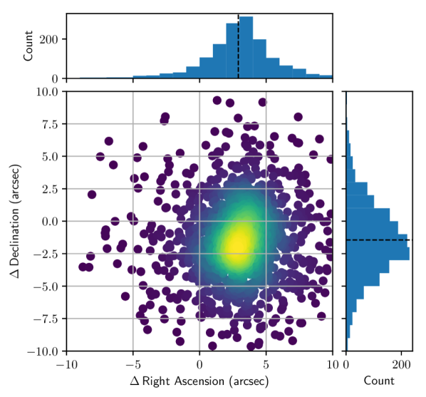
Figure 7: Positional difference (MOST – ASKAP) of 1509 sources found in both the 843 MHz (MOST) and the 960 MHz catalogues. The mean offsets are $\Delta$RA=+2.90″ (SD=2.65) and $\Delta$DEC=–1.45″ (SD=2.92).

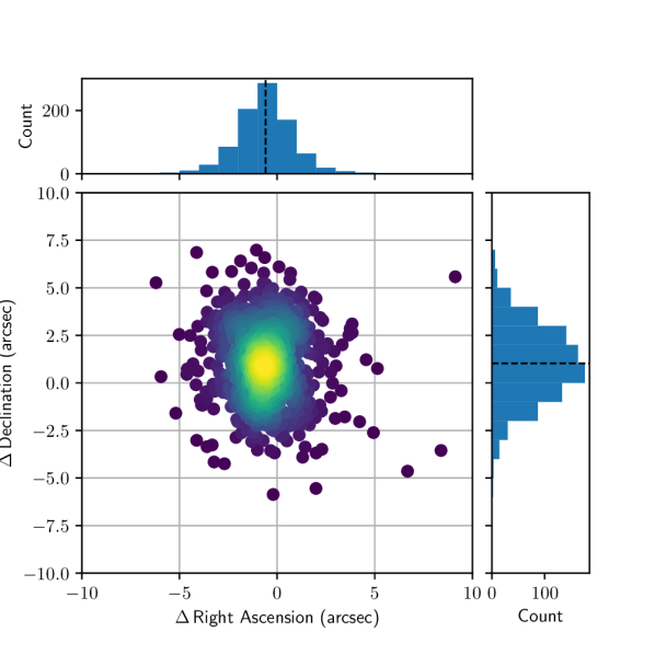
Figure 8: Positional difference (ATCA – ASKAP) of 889 sources found in both the 1320 MHz and the 1400 MHz (ATCA) catalogues. The mean offsets are

$\Delta$RA=–0.58″ (SD=1.50) and $\Delta$DEC=+1.03″ (SD=1.95).

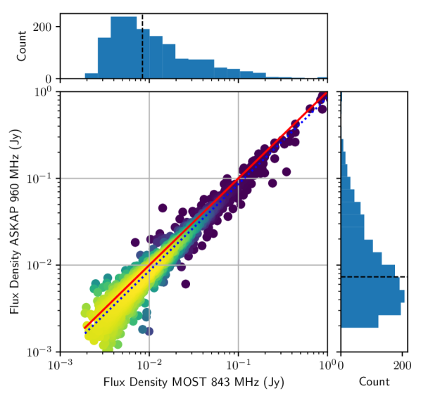
Figure 9: Integrated flux density comparison of sources found in both the 960 MHz and the 843 MHz catalogues. The best fit slope (linear) is 0.89$\pm$0.01 (dotted blue) while the red line represent 1-to-1 ratio (see Section 3.3). The points are colour coded to indicate local density, yellow for high density through to purple for low density. The source integrated flux density distributions are shown in the side and top panels, with the black dashed line at the median integrated flux density.

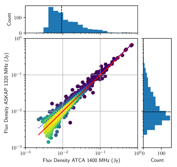
Figure 10: Integrated flux density comparison of sources found in both the 1320 MHz and the 1400 MHz catalogues. The best fit slope (linear) is 0.99$\pm$0.01 (dotted blue) while red line represent 1-to-1 ratio (see Section 3.3). The points are colour coded to indicate local density, yellow for high density through to purple for low density. The source integrated flux density distributions are shown in the side and top panels, with the black dashed line at the median integrated flux density.

Finally, we estimate the radio spectral index for all sources in common and show their distribution in Figure 11. There are 4114 sources found at only two frequencies (marked in red; Figure 11) and for those we estimate a mean $\alpha$ of –0.84. For 1611 sources that are found in three different catalogues (marked in blue; Figure 11) we found a mean $\alpha$ of –0.81 (SD=1.35). We also estimate the average $\alpha$ for sources that are detected in four (927 sources; purple; Figure 11; $\alpha$=–0.71, SD=0.75), five (569 sources; grey; Figure 11; $\alpha$=–0.71, SD=0.59), six (412 sources; orange; Figure 11; $\alpha$=–0.67, SD=0.72) and seven (172 sources; green; Figure 11; $\alpha=-0.54$, SD=0.51) different frequencies. Given that our sample sizes of SNRs, PNe and H ii regions are around 100-150 (see Sections 4 and 5), this distribution is as expected and indicates that the vast majority of our sources from Table 4 are most likely to be background objects (see e.g. Filipović et al., 1998; Collier et al., 2018; Galvin et al., 2018). We note that some sources with flux density measurements at more than two frequencies might exhibit spectral curvature and therefore the fitted value of alpha would not represent a good estimate.

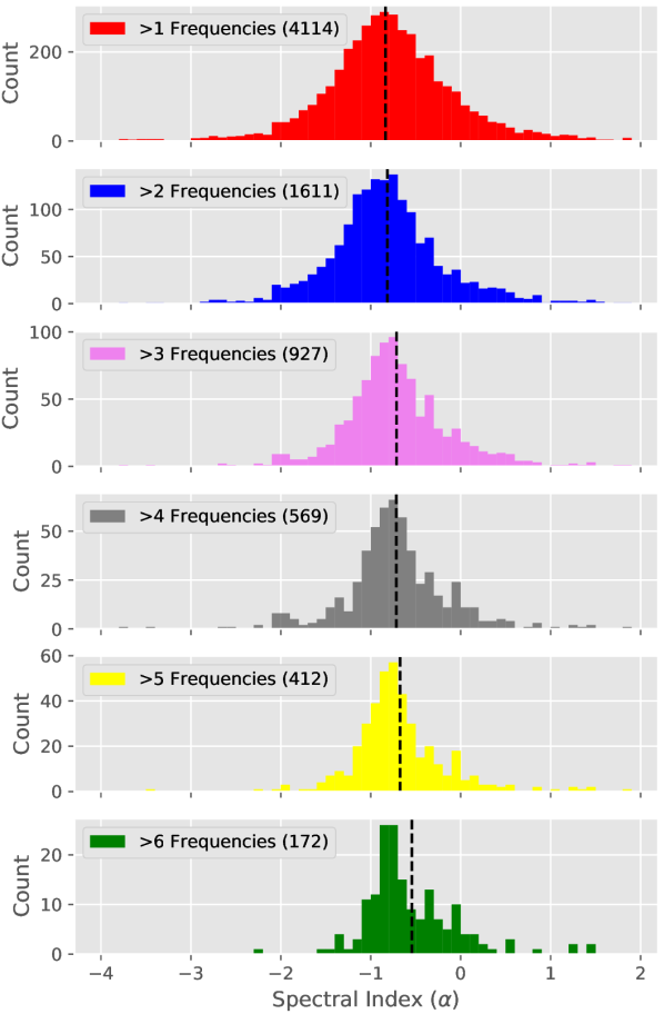
Figure 11: Spectral index distribution of all sources in the field of SMC binned at 0.1. The vertical dashed line represents the mean $\alpha$ of each panel, as discussed in Section 3.3. The uppermost panel includes all the sources of the other panels beneath.

4 ASKAP SMC supernova remnant Sample

Because of their proximity and location well away from the Galactic Plane, we are able to study the sources belonging to the MCs, such as the supernova semnant (SNR) population. Together, these galaxies offer the opportunity to produce a complete sample of SNRs suitable for population studies focused on size, evolution, radio spectral index and beyond, as shown by Maggi et al. (2016) and Bozzetto et al. (2017). To that end, one of our prime goals with the next generation of ASKAP surveys is to detect new and predominantly low surface brightness SNRs. Indeed, with its unique coverage and depth, this new ASKAP ESP survey allowed us to search for new SNRs and at the same time, measure the physical properties of the already established SNRs, examples of which are shown in Figures 3 and 4.

Previous studies of SNRs in the SMC (Filipović et al., 2005; Payne et al., 2007; Owen et al., 2011; Haberl et al., 2012b; Crawford et al., 2014; Roper et al., 2015; Alsaberi et al., 2019; Gvaramadze et al., 2019; Sano et al., 2019) have established 19 objects as bona-fide SNRs with two more considered as good candidates. These two SNR candidates are not detected in our radio images and we will discuss them in our subsequent papers.

Here, we present our radio continuum study results which suggest two new sources to be SNR candidates (MCSNR J0057–7211 and MCSNR J0106–7242), bringing our sample of SMC SNRs and SNR candidates to 23. At the same time, we measure integrated flux densities for 18 of the 19 known SMC SNRs (see Table LABEL:tbl:snr) and present our integrated flux density estimates for the two new SMC SNR candidates found in our new ASKAP SMC surveys (Table LABEL:tbl:snrcan). An in-depth study of the SMC SNR population will be presented in Maggi et al. (submitted, https://arxiv.org/abs/1908.11234).

These two new SNR candidates were initially selected purely based on their typical morphological appearance (circular shape). As our SMC SNR sample is morphologically diverse, various approaches (and initial parameters) were employed in order to measure the best SNR flux densities. Namely, we used the miriad (Sault et al., 1995) task imfit to extract integrated flux density, extensions (diameter/axes) and position angle for each radio detected SNR. For cross checking and consistency, we also used aegean and found no significant difference in integrated flux density estimates.

We used two methods: For SNRs which are known point sources (such as SNR 1E 0102.2–7219, which is not resolved in radio) we use simple Gaussian fitting which produced the best result. The second approach was applied to all resolved SNRs. For those, we measured their local background noise (1$\sigma$) and carefully select the exact area of the SNR. We then estimated the sum of all brightnesses above 5$\sigma$ of each individual pixel within that area and converted it to SNR integrated flux density following Findlay (1966, eq. 24). We also made corrections for an extended background where applicable i.e. for sources where nearby extended object such as H ii region(s) is evident. However, for the most of our SMC SNRs this extended background contribution is minimal.

The two new SNR candidates are shown in Figs. 12 and 13 and their integrated flux density measurements in Table LABEL:tbl:snrcan. These two new SNR candidates display approximately semi-circular structures consistent with a typical spherical morphology. As expected, they are both of low radio surface brightness, which is the main reason for their previous non-detection. We estimate the spectral index for both objects (Table LABEL:tbl:snrcan) and they are consistent with typical SNR spectra, as found in, for example, the larger Large Magellanic Cloud (LMC) population (see Fig. 13 in Bozzetto et al., 2017). Therefore, in addition to their typical morphology, their radio spectral index points to a non-thermal origin which further supports that these objects be classified as SNR candidates. Neither of these two SNR candidates are detected at optical or Infrared (IR) wave bands, which is not unusual given that a number of previously known bona-fide SNRs have only been seen at one wavelength (Filipović et al., 2008).

New ASKAP SNR candidate MCSNR J0057$-$7211 (also see Ye et al., 1991) is located inside the ellipse around XMMU J0057.7–7213 (on the northern side, see Fig. 6 in Haberl et al., 2012b). The nearby point source XMMU J005802.4–721205 is listed as an Active Galactic Nuclei (AGN) candidate (Sturm et al., 2013). Also, there is a moderately bright, point-like X-ray source at 00:58:02.604, $-$72:12:06.7 with a non-thermal spectrum and $L_{\rm{X}}\sim 10^{34}$ erg s^-1 (Haberl et al., 2012b).

On inspection of present generation XMM–Newton mosaic images, we find diffuse emission at the position of the second ASKAP SMC SNR candidate – MCSNR J0106$-$7242. A more comprehensive study of the whole SMC SNR population will be presented in an upcoming study by Maggi et al. (in prep.).

We also use the equipartition formulae (Arbutina et al., 2012, 2013; Urošević et al., 2018) to estimate the magnetic field strength for these two SNR candidates. While this derivation is purely analytical, we emphasise that it is formulated especially for the estimation of the magnetic field strength in SNRs. The average equipartition field over the whole shell of MCSNR J0057–7211 is $\sim$15 $\mu$G while estimates for MCSNR J0106–7242 are around $\sim$8 $\mu$G, with an estimated minimum energy of E_min=6$\times 10^{49}$ erg and E_min=1.5$\times 10^{49}$ erg, respectively. These values are typical of older SNRs at the end of the Sedov phase where the magnetic field is three to four times more compressed than that of middle-age SNRs.

The position of these two SNR candidates on the surface brightness to diameter ($\Sigma$–D) diagram ($\Sigma$= 6.38$\times 10^{-22}$ W m^-2 Hz^-1 sr^-1 and 5.38$\times 10^{-22}$ W m^-2 Hz^-1 sr^-1, D=47 pc and 44.9 pc, respectively) by Pavlović et al. (2018), suggests that these remnants are in the late Sedov phase, with an explosion energy of 1–2$\times 10^{51}$ erg, which evolves in an environment with a density of 0.02–0.2 cm^-3.

Table 7: 19 SNRs in the SMC. Only MCSNRJ0103–7201 is not detected in our ASKAP ESP images. The integrated flux density errors are $<$10 per cent. Column 2 (Other Name) abbreviations are: DEM S: Davies et al. (1976), [HFP2000]: Haberl et al. (2000), IKT: Inoue et al. (1983), SXP: Haberl et al. (2012a).

MCSNR	Other	RA	DEC	$S_{960\,\mathrm{MHz}}$	$S_{1320\,\mathrm{MHz}}$
Name	Name	(J2000)	(J2000)	(Jy)	(Jy)
J0041–7336	DEM S5	00 41 01.7	$-$73 36 30.4	0.138	0.130
J0046–7308	[HFP2000] 414	00 46 40.6	$-$73 08 14.9	0.111	0.110
J0047–7308	IKT 2	00 47 16.6	$-$73 08 36.5	0.441	0.381
J0047–7309		00 47 36.5	$-$73 09 20.0	0.201	0.185
J0048–7319	IKT 4	00 48 19.6	$-$73 19 39.6	0.121	0.092
J0049–7314	IKT 5	00 49 07.7	$-$73 14 45.0	0.068	0.060
J0051–7321	IKT 6	00 51 06.7	$-$73 21 26.4	0.085	0.096
J0052–7236	DEM S68	00 52 59.9	$-$72 36 47.0	0.091	0.081
J0058–7217	IKT 16	00 58 22.4	$-$72 17 52.0	0.079	0.070
J0059–7210	IKT 18	00 59 27.7	$-$72 10 09.8	0.559	0.502
J0100–7133	DEM S108	01 00 23.9	$-$71 33 41.1	0.161	0.146
J0103–7209	IKT 21	01 03 17.0	$-$72 09 42.5	0.100	0.085
J0103–7247	[HFP2000] 334	01 03 29.1	$-$72 47 32.6	0.0288	0.025
J0103–7201		01 03 36.6	$-$72 01 35.1	–	–
J0104–7201	1E 0102.2-7219	01 04 01.2	$-$72 01 52.3	0.402	0.272
J0105–7223	IKT 23	01 05 04.2	$-$72 23 10.5	0.102	0.095
J0105–7210	DEM S128	01 05 30.5	$-$72 10 40.4	–	0.050
J0106–7205	IKT 25	01 06 17.5	$-$72 05 34.5	0.0095	0.0090
J0127–7333	SXP 1062	01 27 44.1	$-$73 33 01.6	0.0072	0.0068

Table 8: Details of two new ASKAP SNRs candidates in the SMC. The integrated flux density errors are $<$10 per cent. N S abbreviation stands as at Henize (1956)

.
MCSNR Other RA DEC $S_{960\,\mathrm{MHz}}$ $S_{1320\,\mathrm{MHz}}$ $\alpha\pm\Delta\alpha$ Name Name (J2000) (J2000) (Jy) (Jy) J0057–7211 N S66D 00 57 49.9 $-$72 11 47.1 0.030 0.0244 –0.75$\pm$0.04 J0106–7242 01 06 32.1 $-$72 42 17.0 0.024 0.020 –0.55$\pm$0.02

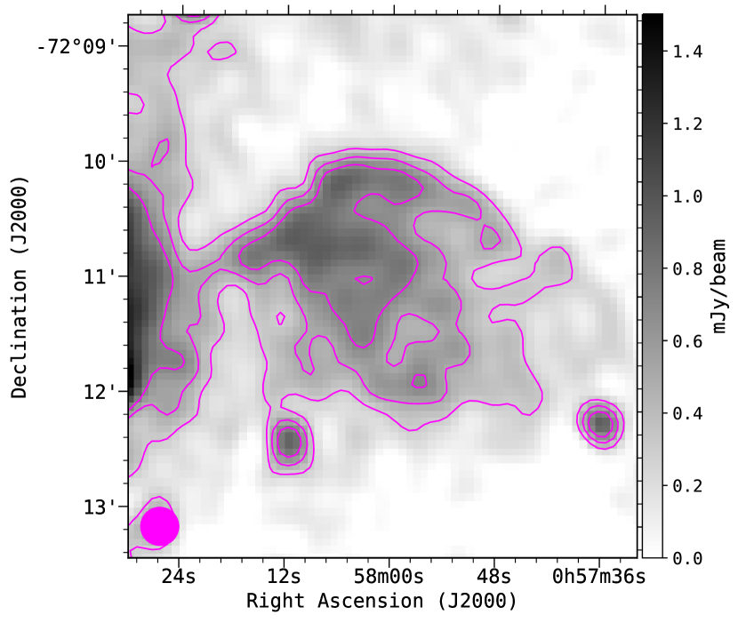
Figure 12: ASKAP ESP image of the new SMC SNR candidate MCSNR J0057-7211 at 1320 MHz (grey scale and contours) smoothed to a resolution of 20″$\times$ 20″. Magenta contours are: 0.3, 0.5, and 0.7 mJy beam^-1. The smoothed beam is shown as a filled magenta circle in the lower left corner. Two point-like sources in the lower right and left corner are unrelated background sources. The local RMS noise is 0.1 mJy beam^-1.

Figure 13: ASKAP ESP image of the new low surface brightness SMC SNR candidate MCSNR J0106-7242 at 1320 MHz (grey scale and contours) smoothed to a resolution of 20″$\times$ 20″. Magenta contours are: 0.18, 0.27, 0.36, 0.45 and 0.54 mJy beam^-1. The smoothed beam is shown as a filled magenta circle in the lower left corner. The point-like source in the upper right corner is an unrelated background source. The local RMS noise is 0.06 mJy beam^-1.

5 ASKAP SMC Planetary Nebula Sample

The location and proximity of the SMC also provides an opportunity to create a complete sample of radio continuum detected planetary nebulae (PNe) in that nearby galaxy. PNe are important for studies of the chemical, atomic, molecular and solid-state galactic ISM enrichment (Kwok, 2005, 2015). The next generation ASKAP surveys aim to provide detection of lower surface brightness planetary nebula (PN) to help complete the SMC PN sample.

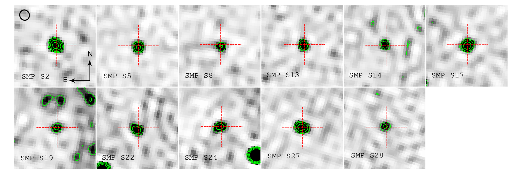
Figure 14: Finding charts of 11 SMC PNe with positive detection at 1320 MHz. Each field is 2 arcmin in size and the grey-scale uses the same sinh stretching. The approximate shape of the synthesized beam and orientation of each chart is displayed in the upper left corner. Red cross represents the catalogued position of a PN and green contours are radio continuum intensity at 3, 5, 8 and 12$\times$ RMS noise measured in the vicinity of the object. Here, we present only objects with 5$\sigma$ detections for which we measured accurate flux densities. N is up and E is left in each panel.

Previous searches for radio PNe in the SMC (Payne et al., 2008; Filipović et al., 2009; Bojičić et al., 2010; Leverenz et al., 2016) yielded 16 bona-fide PN detections. Our ASKAP ESP survey has revealed 6 new PN radio detections (see Table 9) reported here for the first time (Figure 14), bringing the total number of known SMC PNe detected in radio to 22. Our new data contribute 18 new accurate radio continuum flux density measurements from ASKAP on this sample (excluding dubious detections and upper flux limits), of which 7 are at 960 MHz and 11 at 1320 MHz.

All finding charts created here have been visually inspected for a possible detection. Of 102 true, likely and possible SMC PNe in our base catalogue we have matched 17 radio counterparts with peak emission over three times the local noise in the 1320 MHz map and 8 in the 960 MHz map. The flux densities were measured using the Gaussian fitting method imfit from casa (McMullin et al., 2007). Since none of the SMC PNe are expected to be resolved based on their known optical size, the Gaussian fitting was constrained to the beam size, effectively measuring the peak of the emission. Calculations of uncertainties for this method are based on Condon (1997) and have been adopted directly from imfit’s output. We visually inspected all possible detections with a peak brightness over $F\geq 3\sigma$ using a comparison between the original and the residual maps.

The results are presented in Table 9 and Figure 14. Out of 17 detections at 1320 MHz, we measured accurate flux densities for 11 PNe with peak brightness over 5$\sigma$. Likewise, in the 960 MHz band we accurately measured 7 out of 8 detected PNe. We flagged PNe with the peak brightness below 5$\sigma$ in Table 9 with a value in parentheses. The flux density estimates for these PNe can be considered only as upper limits.

We modelled 5 GHz flux densities for all detected PNe in order to construct a radio continuum spectrum distribution of radio-detected SMC PNe. The flux modelling was performed as follows: a) if more than 2 data points were available we apply free-free emission spectral energy modelling ( Spectral Energy Distribution (SED); see further text), b) if only one or two data points were measured, we estimated the 5 GHz integrated flux density from the measurements at the frequency or frequencies available by applying a simple power law approximation i.e. $S_{5GHz}=S_{\nu}\cdot(5/\nu[\text{GHz}])^{-0.1}$.

For SED modelling we used a spherical shell model with a constant electron density in the shell ($n_{e}$), outer radius ($R_{\text{out}}$) and inner radius ($R_{\text{in}}$). The model can now be applied to measured data points with:

$$S_{\nu}=\frac{4\pi kT_{e}\nu^{2}}{c^{2}D^{2}}R_{\text{out}}^{2}\int_{0}^{\infty}x(1-e^{-\tau_{\nu}\cdot g_{1}(x)})dx$$ (1)

where $\tau_{\nu}$ is the optical thickness through the centre of the nebula at frequency $\nu$ which, for an assumption of $n_{e}=const$ and a pure hydrogen isothermal plasma, can be approximated with $\tau_{\nu}\approx 8.235\cdot 10^{-2}T_{e}^{-1.35}\nu^{-2.1}n_{e}^{2}\cdot 2(R_{\text{out}}-R_{\text{in}})$. Finally, the function $g(x)$ describes the geometry of the nebula (see Olnon, 1975, for more details). For this model $g(x)$ has a form:

$$\begin{split}g_{1}(x)&=\sqrt{1-x^{2}}-\sqrt{\mu^{2}-x^{2}}&\text{for}~{}x<\mu,\\ &=\sqrt{1-x^{2}}&\text{for}~{}\mu\leq x<1~{}\text{and}\\ &=0&\text{for}~{}x\geq 1,\\ \end{split}$$ (2)

where $\mu=R_{\text{in}}/R_{\text{out}}$ i.e. inner to outer radii ratio. We fixed the electron temperature to its canonical value ($T_{e}=10^{4}$ K) and $\mu=0.4$ as this is found to be the expected average value for majority of Galactic PNe (Schönberner et al., 2007; Marigo et al., 2001). With an assumed distance to the SMC of 60 kpc we fit the two free parameters, $R_{\text{out}}$ and the emission measure ($EM$), through the centre of the nebula. Finally, the model shown here has been used to estimate the integrated flux density at 5 GHz.

In Fig. 15 we show graphical results of the SED fitting. From the six PNe with an adequate number of data points to apply our spherical shell model, only four converged to acceptable values of $R_{\text{out}}$ and $EM$. For two PNe (SMP S14 and SMP S22) the model failed to converge and the data were fitted with the simple power law $S_{\nu}\sim\nu^{\alpha}$. The spectral indices ($\alpha$) obtained are –0.09 and –0.1 for SMP S14 and SMP S22, respectively.

We present the modelled 5 GHz total flux densities in Table 9 (Column 11). The distribution of the modelled 5 GHz total flux densities for the detected sample is presented in Fig. 16. It can be seen that the number of PNe drops down below 0.6 mJy which is approximately the detection limit for ASKAP ESP data. Objects detected below this limit are either upper limits or detections originating from high sensitivity ATCA observations (Wong et al., 2011b). Therefore, we believe that our sample of radio detected SMC PNe is now complete down to $\sim$0.6 mJy. We have used this distribution to roughly estimate the number of SMC PNe which will be detectable in future ASKAP observations of the SMC.

With the approximation that PNe are fully ionised spherical shells of constant mass, expanding with constant velocity and ionised by a non-evolving central star (Henize & Westerlund, 1963) the optically thin radio continuum flux would behave as $F\propto~{}R(t)^{-3}\propto~{}t^{-3}$. Although simplistic, this approximation has proven to be quite effective in describing changes in flux from Balmer lines during the expansion phase in a large number of observationally constructed PN luminosity functions (Reid & Parker, 2010; Ciardullo, 2010).

Using a sample of radio catalogued Galactic Bulge PNe, Bojičić (2010) showed that the theoretical shape of the PNLF (Ciardullo et al., 1989) effectively describes the distribution of radio flux densities of PNe at a known distance. Using our assumption that the SMC PN radio sample is now complete down to 0.6 mJy, we have used the theoretical shape of the PNLF to estimate the distribution of 5 GHz integrated flux densities below the ASKAP ESP detection limit (more details in Bojičić et al. 2019, in prep.). We fit the truncated exponential function (Ciardullo et al., 1989) to the obtained distribution of log${}_{10}(S_{\rm{5GHz}})$ fluxes (in mJy). The data is binned to 0.2 dex in log flux density and we have used only bins containing PNe with $S_{\rm{5GHz}}>0.6$ mJy for the fit. The estimated rough model is over-plotted on the resulting histogram (Figure 16; dashed line). Finally, we anticipate that increasing the sensitivity by an order of magnitude would allow detection of another 20 SMC PNe, while reaching a 10 $\mu$Jy beam^-1 (Norris et al., 2011) will allow us to increase the number of detections to $\approx 120$ PNe i.e. over 50 per cent of the expected SMC PNe population (Jacoby & De Marco, 2002).

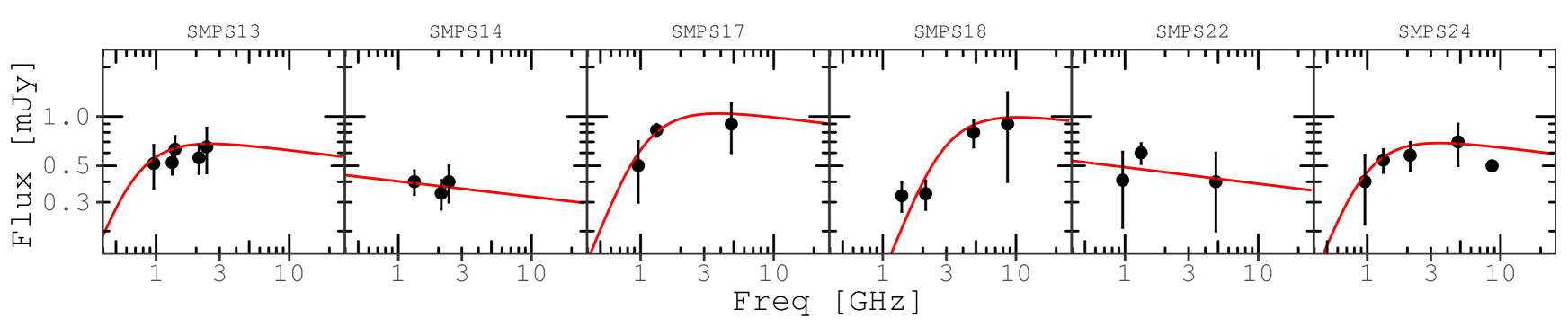
Figure 15: Best fit model SEDs to the observed flux densities for 6 SMC PNe with three or more available and good data points.

Figure 16: Planetary nebulae luminosity function (PNLF) for the SMC. The dashed line represents the theoretical PNLF estimated assuming the sample is complete down to 0.6 mJy.

Table 9: Radio continuum population of PNe in the SMC. The new ASKAP radio continuum detection and integrated flux density measurements of the SMC PNe are indicated with ^†. Uncertain detections and upper and lower limits in flux estimates are indicated in flux columns with :, $<$ and $>$, respectively. The integrated flux density errors are $<$10 per cent unless otherwise stated.

			ATCA	ATCA	ATCA	ATCA-CABB	ATCA	ASKAP	ASKAP	model
Other	RA	DEC	$S_{3\,\mathrm{cm}}$	$S_{6\,\mathrm{cm}}$	$S_{13\,\mathrm{cm}}$	$S_{2.1\,\mathrm{GHz}}$	$S_{20\,\mathrm{cm}}$	$S_{23\,\mathrm{cm}}$	$S_{32\,\mathrm{cm}}$	$S_{6\,\mathrm{cm}}$
Name	(J2000)	(J2000)	8640 MHz	4800 MHz	2400 MHz	2100 MHz	1388 MHz	1320 MHz	960 MHz	5000 MHz
			(mJy)	(mJy)	(mJy)	(mJy)	(mJy)	(mJy)	(mJy)	(mJy)
(1)	(2)	(3)	(4)	(5)	(6)	(7)	(8)	(9)	(10)	(11)
SMP S2†	00:32:39	$-$71:41:59.5	…	…	…	…	(2)	1.25$\pm$0.08	1.1$\pm$0.2	1.1
SMP S3†	00:34:22	$-$73:13:21.5	…	…	…	…	…	(0.3)	(0.4)	0.3
SMP S5†	00:41:22	$-$72:45:16.8	…	…	…	…	…	0.67$\pm$0.08	0.3$\pm$0.2	0.6
SMP S6	00:41:28	$-$73:47:06.4	1.1$\pm 0.5$	1.3$\pm 0.1$	…	…	>0.2	…	…	1.2
SMP S8†	00:43:25	$-$72:38:18.8	…	…	…	…	…	0.43$\pm$0.08	…	0.4
SMP S9	00:45:21	$-$73:24:10.0	…	…	…	0.15	…	…	…	0.1
SMP S10†	00:47:00	$-$72:49:16.6	…	…	…	…	(0.3)	(0.4)	…	0.2
SMP S13†	00:49:52	$-$73:44:21.7	…	…	0.7$\pm 0.2$	0.56	…	0.52$\pm$0.08	0.52$\pm$0.15	0.6
SMP S14†	00:50:35	$-$73:42:57.9	…	…	0.4$\pm 0.1$	0.34	…	0.40$\pm$0.06	…	0.4
SMP S16†	00:51:27	$-$72:26:11.7	…	0.6$\pm 0.1$	…	…	…	<0.4	…	0.6
J18	00:51:43	$-$73:00:54.5	…	…	0.24	…	…	…	…	0.2
SMP S17†	00:51:56	$-$71:24:44.2	…	0.9$\pm 0.3$	…	…	…	0.82$\pm$0.07	0.5$\pm$0.2	0.9
SMP S18†	00:51:58	$-$73:20:31.9	0.9$\pm 0.5$	0.8$\pm 0.15$	…	0.34	0.3	(0.3)	…	0.8
SMP S19†	00:53:11	$-$72:45:07.6	…	…	0.6$\pm 0.2$	…	…	0.36$\pm$0.08	…	0.6
MA891	00:55:59	$-$72:14:00.3	…	…	…	0.92	…	…	…	0.8
LIN 302†	00:56:19	$-$72:06:58.5	…	…	…	0.11	…	(0.3)	…	0.1
SMP S21	00:56:31	$-$72:27:02.0	…	…	…	0.21	…	…	…	0.2
SMP S22†	00:58:37	$-$71:35:48.8	…	0.4$\pm 0.2$	…	…	…	0.60$\pm$0.08	0.4$\pm$0.2	0.4
SMP S23†	00:58:42	$-$72:56:59.9	…	…	…	…	…	(0.4)	…	0.3
SMP S24†	00:59:16	$-$72:01:59.8	0.5	0.7$\pm 0.2$	…	0.58	…	0.54$\pm$0.09	0.4$\pm$0.2	0.7
SMP S27†	01:21:11	$-$73:14:34.8	…	…	…	…	…	0.88$\pm$0.08	0.68$\pm$0.10	0.8
SMP S28†	01:24:12	$-$74:02:32.3	…	…	…	…	…	0.32$\pm$0.07	…	0.3

6 Other interesting sources

In Sections 4 and 5 we investigated SNRs and PN populations within the SMC. Large SMC H ii region complexes N 19 and N 66 are shown in Figures 3 and 4. Together with other SMC H ii regions and YSOs, they will be further investigated in our subsequent papers.

We would also like to highlight some sources of interest behind the SMC that are worth following up. Due to their complex radio structure they are probes of galaxy interactions or interaction with the environment. These are presented in Figures 17, 18, 19, 20 and 21 and would fall into the category of extended radio AGN.

One of the most interesting sources behind the SMC revealed by our ASKAP observations is the radio AGN shown in Figure 17. This object displays a set of radio lobes associated to the an infrared IRAC source (background of Figure 17). Also associated with the same source seems to be a radio jet with direction pointing towards the observer. Over the past year there has been a multi-wavelength effort to reveal of the true nature behind this peculiar radio structure, which might be linked to a binary supermassive black hole. Still we cannot rule out chance coincidence. Scheduled follow-up observations, with ATCA (PI: Vardoulaki) and SALT (PI: van Loon), will help shed light to the nature of this interesting radio source.

Other sources also show complex AGN structures with various morphological types (Figures 19 and 20) (see also O’Brien et al., 2018) and sizes, including a bent source in a possible galaxy cluster (Figure 18). Such morphology of the extended radio emission, is expected from binary driven jets. A similar configuration is also seen toward other Super Massive Black Hole (SMBH)s, such as OJ 287 (Kushwaha et al., 2019). The object in Figure 21 is a slightly bent FR-I type radio galaxy, possibly the central part of a Wide-Angle Tail (WAT) in a cluster of galaxies.

We also examined seven Flat Spectrum Radio Quasars (FSRQs) and BL Lacertae (BL-Lac) candidates from Żywucka et al. (2018) in our radio catalogues. We found that objects J0111$-$7302 (proposed BL-Lac.; Figure 23) and possibly J0120$-$7334 (proposed FSRQs; Figure 22) exhibit typical FR-I morphology with complex but steep spectral indices which would argue for their AGN nature. The other five sources listed in Żywucka et al. (2018) are point-like radio sources in our catalogues: J0039$-$7356 (BL-Lac; $\alpha=-1.1$), J0054$-$7248 (FSRQs; detected only at 1320 MHz), J0114$-$7320 and J0122$-$7152 (both proposed FSRQs but we detect as a complex AGN with jets) and J0123$-$7236 (BL-Lac; $\alpha=-0.7$). In addition, we found four radio sources in our catalogue that correspond to the Visual and Infrared Survey Telescope for Astronomy (VISTA; Emerson et al., 2006), survey of the MCs (VMC; Cioni et al., 2011) and spectroscopically confirmed quasars (Ivanov et al., 2016). They are J0027$-$7223 (S${}_{1320\,\rm{MHz}}$=0.265 mJy), J0029$-$7146 ($\alpha=-1.0$), J0035$-$7201 ($\alpha=-0.5$) and J0119$-$7348 ($\alpha=-0.8$). While small, this sample exhibits steep spectral indices typical of the majority of background radio objects.

Finally, we note a radio detection of an ultra-bright submillimeter galaxy MM J01071$-$7302 (Takekoshi et al., 2013) and found a steep spectrum with $\alpha=-0.9$.

In total, we found 7736 point radio sources with fluxes over 5 times the local noise, the vast majority of which are likely to be in the background of the SMC. Through absorption measurements, all these sources can provide excellent probes for the study of cold gas in both SMC and the Galaxy (e.g. Li et al., 2018; McClure-Griffiths et al., 2015; Dickey et al., 2013). A more detailed analysis of these background sources will be presented in Pennock et al. (in prep.).

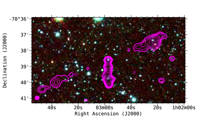
Figure 17: ASKAP ESP image (contours) of the possible double black hole AGN. The background image is a three-colour IRAC composite with 8.0, 4.5 and 3.6 µm represented as red, green and blue, respectively. The magenta radio contours are from our 1320 MHz survey drawn at 0.25, 0.3, 0.5, 0.7, 1, 1.5, 2, 3 and 5 mJy beam^-1. The 1320 MHz radio beam size of 16.3″ $\times$ 15.1″ is shown as a filled magenta ellipse in the lower left corner.

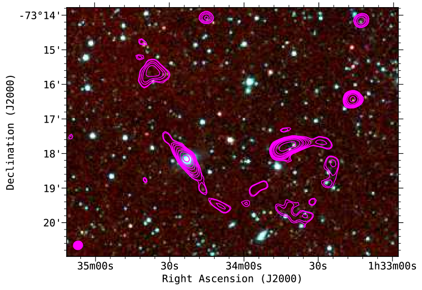
Figure 18: ASKAP ESP image (contours) shows a long, twisted structure that appears to be a highly distorted tailed radio galaxy associated with 2MASX J01342297–7318113, a bright galaxy (V=15.9 mag) without spectroscopic redshift. Although the multiple bends might suggest that there is actually more than one radio source, there is no obvious second optical/IR host. The bright compact object near the centre of the radio source elongated E-W and $\sim$3 arcmin W of 2MASX J01342297–7318113, is 2MASS J01334172–7317527, but GaiaDR2 (Gaia Collaboration et al., 2018) shows it to be a star with significant parallax and proper motion. The background image is a three-colour IRAC composite with 8.0, 4.5 and 3.6 µm represented as red, green and blue, respectively. The magenta radio contours are from our 1320 MHz survey drawn at 0.25, 0.3, 0.5, 0.7, 1, 1.5, 2, 3 and 5 mJy beam^-1. The 1320 MHz beam size of 16.3″ $\times$ 15.1″ is shown as a filled magenta ellipse in the lower left corner.

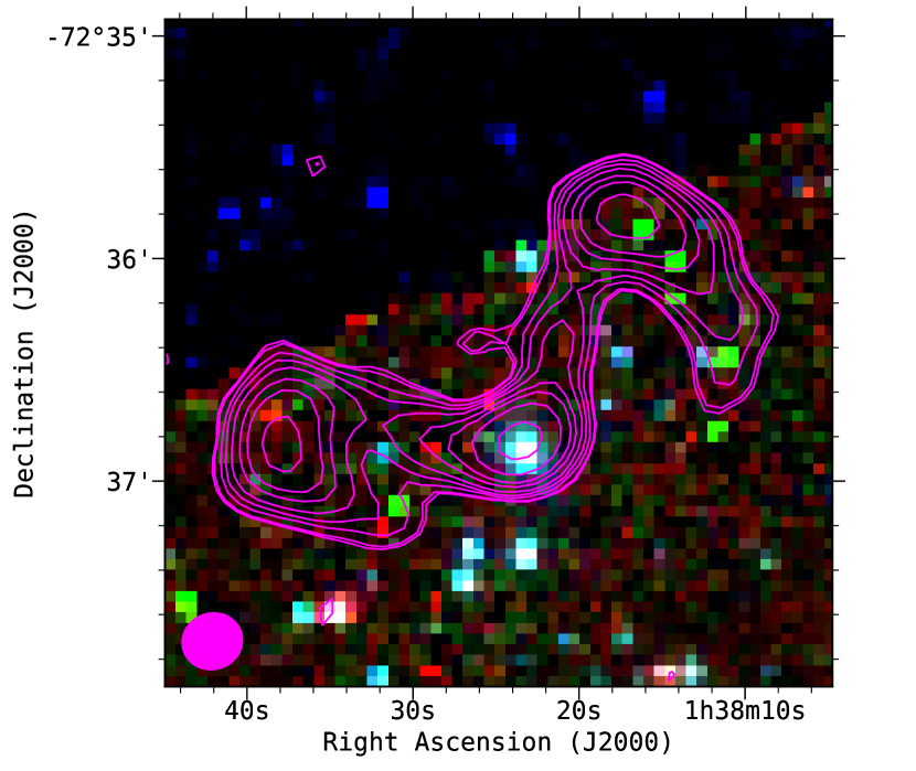
Figure 19: ASKAP ESP image of the “duck” AGN complex or possible bent-tail radio galaxy. The background image is a three-colour IRAC composite with 8.0, 4.5 and 3.6 µm represented as red, green and blue, respectively. The magenta radio contours are from our 1320 MHz survey drawn at 0.25, 0.3, 0.5, 0.7, 1, 1.5, 2, 3 and 5 mJy beam^-1. The 1320 MHz beam size of 16.3″ $\times$ 15.1″ is shown as a filled magenta ellipse in the lower left corner.

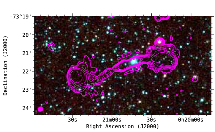
Figure 20: ASKAP ESP image of the FR-II AGN. The background image is a three-colour IRAC composite with 8.0, 4.5 and 3.6 µm represented as red, green and blue, respectively. The magenta radio contours are from our 1320 MHz survey drawn at 0.25, 0.3, 0.5, 0.7, 1, 1.5, 2, 3 and 5 mJy beam^-1. The 1320 MHz beam size of 16.3″ $\times$ 15.1″ is shown as a filled magenta ellipse in the lower left corner.

Figure 21: ASKAP ESP image of the FR-I AGN. The background image is a three-colour IRAC composite with 8.0, 4.5 and 3.6 µm represented as red, green and blue, respectively. The magenta radio contours are from our 1320 MHz survey drawn at 0.25, 0.3, 0.5, 0.7, 1, 1.5, 2, 3 and 5 mJy beam^-1. The 1320 MHz beam size of 16.3″ $\times$ 15.1″ is shown as a filled magenta ellipse in the lower left corner.

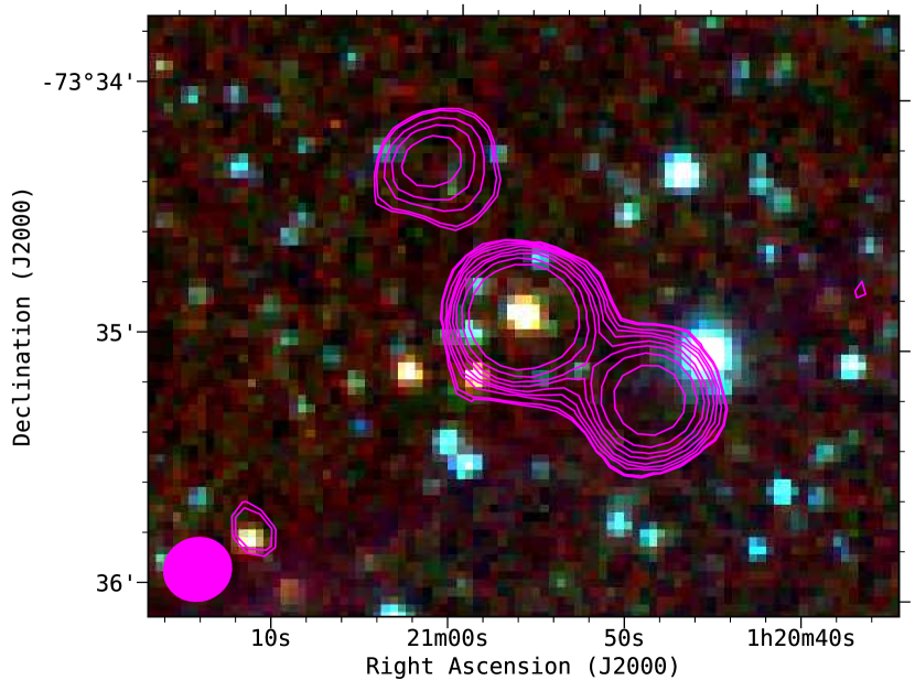
Figure 22: ASKAP ESP image of the possible AGN J0120$-$7334. The background image is a three-colour IRAC composite with 8.0, 4.5 and 3.6 µm represented as red, green and blue, respectively. The yellow radio contours are from our 1320 MHz survey drawn at 0.25, 0.3, 0.5, 1, 2, 3, 5, 10, 20 and 30 mJy beam^-1. The 1320 MHz beam size of 16.3″ $\times$ 15.1″ is shown as a filled magenta ellipse in the lower left corner.

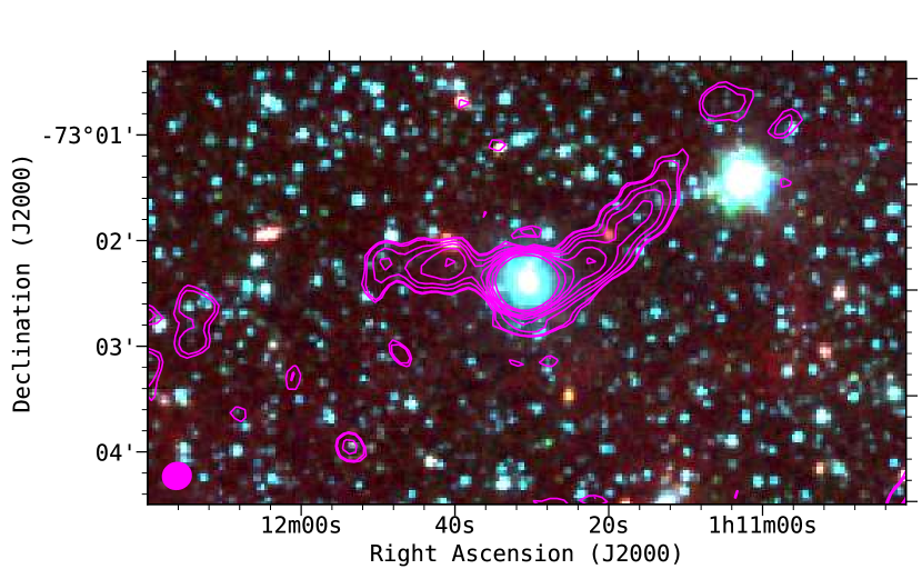
Figure 23: ASKAP ESP image of the AGN complex J0111$-$7302. The background image is a three-colour IRAC composite with 8.0, 4.5 and 3.6 µm represented as red, green and blue, respectively. The yellow radio contours are from our 1320 MHz survey drawn at 0.25, 0.3, 0.5, 1, 2, 3, 5, 10, 20, 30 and 50 mJy beam^-1. The 1320 MHz beam size of 16.3″ $\times$ 15.1″ is shown as a filled magenta ellipse in the lower left corner.

7 Conclusions

In this paper we present the ASKAP EMU ESP radio continuum survey of the SMC taken at 960 MHz and 1320 MHz. Our findings can be summarised as follows:

• This new ASKAP survey is a significant improvement (factor of $\sim$4 in the median RMS) compared to previous ATCA/MOST surveys of the SMC.

• We identify 4489 and 5954 point sources at 960 MHz and 1320 MHz, respectively (Tables 2 and 3), with the majority of these sources detected above the 5$\sigma$ threshold in their respective bands. We also list non-point sources at both ASKAP frequencies in Tables 5 and 6 (282 and 641, respectively).

• Combining our two new ASKAP catalogues with other radio continuum surveys, we found 7736 point-like sources in common which we list in Table 4, together with spectral indices we determined from all available survey data.

• Two new low surface brightness SNR candidates were discovered, bringing the total number of SNRs and SNR candidates in the SMC to 23.

• Radio counterparts to 22 optically known PNe were detected. This sample of PNe is complete down to 0.6 mJy.

References

- Alsaberi et al. (2019) Alsaberi R. Z. E., et al., 2019, MNRAS, 486, 2507
- Arbutina et al. (2012) Arbutina B., Urošević D., Andjelić M. M., Pavlović M. Z., Vukotić B., 2012, The Astrophysical Journal, 746, 79
- Arbutina et al. (2013) Arbutina B., Urošević D., Vučetić M. M., Pavlović M. Z., Vukotić B., 2013, ApJ, 777, 31
- Bojičić (2010) Bojičić I., 2010, PhD thesis, Macquarie University
- Bojičić et al. (2010) Bojičić I. S., Filipović M. D., Crawford E. J., 2010, Serbian Astronomical Journal, 181, 63
- Bozzetto et al. (2017) Bozzetto L. M., et al., 2017, ApJS, 230, 2
- Ciardullo (2010) Ciardullo R., 2010, Publ. Astron. Soc. Australia, 27, 149
- Ciardullo et al. (1989) Ciardullo R., Jacoby G. H., Ford H. C., Neill J. D., 1989, ApJ, 339, 53
- Cioni et al. (2011) Cioni M.-R. L., et al., 2011, A&A, 527, A116
- Clarke (1976) Clarke J. N., 1976, MNRAS, 174, 393
- Collier (2016) Collier J., 2016, PhD thesis, Western Sydney University (Australia
- Collier et al. (2018) Collier J. D., et al., 2018, MNRAS, 477, 578
- Condon (1997) Condon J. J., 1997, PASP, 109, 166
- Cornwell et al. (2011) Cornwell T. J., Humphreys B., Lenc E., Voronkov M., Whiting M. T., 2011, Technical Report 028, Askap-sw-0020: ASKAP science processing
- Crawford et al. (2011) Crawford E. J., Filipović M. D., de Horta A. Y., Wong G. F., Tothill N. F. H., Draskovic D., Collier J. D., Galvin T. J., 2011, Serbian Astronomical Journal, 183, 95
- Crawford et al. (2014) Crawford E. J., Filipović M. D., McEntaffer R. L., Brantseg T., Heitritter K., Roper Q., Haberl F., Urošević D., 2014, AJ, 148, 99
- Davies et al. (1976) Davies R. D., Elliott K. H., Meaburn J., 1976, Mem. RAS, 81, 89
- DeBoer et al. (2009) DeBoer D. R., et al., 2009, IEEE Proceedings, 97, 1507
- Di Teodoro et al. (2019) Di Teodoro E. M., et al., 2019, MNRAS, 483, 392
- Dickey et al. (2013) Dickey J. M., et al., 2013, Publ. Astron. Soc. Australia, 30, e003
- Emerson et al. (2006) Emerson J., McPherson A., Sutherland W., 2006, The Messenger, 126, 41
- Filipović et al. (1997) Filipović M. D., Jones P. A., White G. L., Haynes R. F., Klein U., Wielebinski R., 1997, A&AS, 121, 321
- Filipović et al. (1998) Filipović M. D., Haynes R. F., White G. L., Jones P. A., 1998, A&AS, 130, 421
- Filipović et al. (2002) Filipović M. D., Bohlsen T., Reid W., Staveley-Smith L., Jones P. A., Nohejl K., Goldstein G., 2002, MNRAS, 335, 1085
- Filipović et al. (2005) Filipović M. D., Payne J. L., Reid W., Danforth C. W., Staveley-Smith L., Jones P. A., White G. L., 2005, MNRAS, 364, 217
- Filipović et al. (2008) Filipović M. D., et al., 2008, A&A, 485, 63
- Filipović et al. (2009) Filipović M. D., et al., 2009, MNRAS, 399, 769
- Findlay (1966) Findlay J. W., 1966, ARA&A, 4, 77
- For et al. (2018) For B.-Q., et al., 2018, MNRAS, 480, 2743
- Franzen et al. (2015) Franzen T. M. O., et al., 2015, MNRAS, 453, 4020
- Gaensler et al. (2005) Gaensler B. M., Haverkorn M., Staveley-Smith L., Dickey J. M., McClure-Griffiths N. M., Dickel J. R., Wolleben M., 2005, Science, 307, 1610
- Gaia Collaboration et al. (2018) Gaia Collaboration et al., 2018, A&A, 616, A1
- Galvin et al. (2018) Galvin T. J., et al., 2018, MNRAS, 474, 779
- Gordon et al. (2011) Gordon K. D., et al., 2011, AJ, 142, 102
- Gvaramadze et al. (2019) Gvaramadze V. V., Kniazev A. Y., Oskinova L. M., 2019, MNRAS, 485, L6
- Haberl et al. (2000) Haberl F., Filipović M. D., Pietsch W., Kahabka P., 2000, A&AS, 142, 41
- Haberl et al. (2012a) Haberl F., Sturm R., Filipović M. D., Pietsch W., Crawford E. J., 2012a, A&A, 537, L1
- Haberl et al. (2012b) Haberl F., et al., 2012b, A&A, 545, A128
- Hancock et al. (2012) Hancock P. J., Murphy T., Gaensler B. M., Hopkins A., Curran J. R., 2012, Aegean: Compact source finding in radio images, Astrophysics Source Code Library (ascl:1212.009)
- Hancock et al. (2018) Hancock P. J., Trott C. M., Hurley-Walker N., 2018, Publ. Astron. Soc. Australia, 35, e011
- Haynes et al. (1986) Haynes R. F., Klein U., Wielebinski R., Murray J. D., 1986, A&A, 159, 22
- Henize (1956) Henize K. G., 1956, ApJS, 2, 315
- Henize & Westerlund (1963) Henize K. G., Westerlund B. E., 1963, ApJ, 137, 747
- Hernández-García et al. (2017) Hernández-García L., et al., 2017, A&A, 603, A131
- Hilditch et al. (2005) Hilditch R. W., Howarth I. D., Harries T. J., 2005, MNRAS, 357, 304
- Hotan et al. (2014) Hotan A. W., et al., 2014, Publ. Astron. Soc. Australia, 31, e041
- Inoue et al. (1983) Inoue H., Koyama K., Tanaka Y., 1983, in Danziger J., Gorenstein P., eds, IAU Symposium Vol. 101, Supernova Remnants and their X-ray Emission. pp 535–540
- Ivanov et al. (2016) Ivanov V. D., et al., 2016, A&A, 588, A93
- Jacoby & De Marco (2002) Jacoby G. H., De Marco O., 2002, AJ, 123, 269
- Johnston et al. (2008) Johnston S., et al., 2008, Experimental Astronomy, 22, 151
- Kushwaha et al. (2019) Kushwaha P., de Gouveia Dal Pino E. M., Gupta A. C., Wiita P. J., 2019, arXiv e-prints,
- Kwok (2005) Kwok S., 2005, Journal of Korean Astronomical Society, 38, 271
- Kwok (2015) Kwok S., 2015, Highlights of Astronomy, 16, 623
- Leverenz et al. (2016) Leverenz H., Filipović M. D., Bojičić I. S., Crawford E. J., Collier J. D., Grieve K., Drašković D., Reid W. A., 2016, Ap&SS, 361, 108
- Leverenz et al. (2017) Leverenz H., Filipović M. D., Vukotić B., Urošević D., Grieve K., 2017, MNRAS, 468, 1794
- Li et al. (2018) Li D., et al., 2018, ApJS, 235, 1
- Maggi et al. (2016) Maggi P., et al., 2016, A&A, 585, A162
- Mao et al. (2008) Mao S. A., Gaensler B. M., Stanimirović S., Haverkorn M., McClure-Griffiths N. M., Staveley-Smith L., Dickey J. M., 2008, ApJ, 688, 1029
- Mao et al. (2012) Mao S. A., et al., 2012, ApJ, 759, 25
- Marigo et al. (2001) Marigo P., Girardi L., Groenewegen M. A. T., Weiss A., 2001, A&A, 378, 958
- Mauch et al. (2003) Mauch T., Murphy T., Buttery H. J., Curran J., Hunstead R. W., Piestrzynski B., Robertson J. G., Sadler E. M., 2003, MNRAS, 342, 1117
- McClure-Griffiths et al. (2015) McClure-Griffiths N. M., et al., 2015, Advancing Astrophysics with the Square Kilometre Array (AASKA14), p. 130
- McClure-Griffiths et al. (2018) McClure-Griffiths N. M., et al., 2018, Nature Astronomy, 2, 901
- McConnell (2017) McConnell D., 2017, Technical report, ACES memo 15: Observing with ASKAP: Optimisation for survey speed. CSIRO Australia Telescope National Facility
- McConnell et al. (2016) McConnell D., et al., 2016, Publ. Astron. Soc. Australia, 33, e042
- McGee et al. (1976) McGee R. X., Newton L. M., Butler P. W., 1976, Australian Journal of Physics, 29, 329
- McMullin et al. (2007) McMullin J. P., Waters B., Schiebel D., Young W., Golap K., 2007, in Astronomical data analysis software and systems XVI. p. 127
- Meixner et al. (2006) Meixner M., et al., 2006, AJ, 132, 2268
- Middelberg et al. (2008) Middelberg E., et al., 2008, AJ, 135, 1276
- Murphy et al. (2013) Murphy T., et al., 2013, Publ. Astron. Soc. Australia, 30, e006
- Norris et al. (2006) Norris R. P., et al., 2006, AJ, 132, 2409
- Norris et al. (2011) Norris R. P., et al., 2011, Publ. Astron. Soc. Australia, 28, 215
- O’Brien et al. (2018) O’Brien A. N., Norris R. P., Tothill N. F. H., Filipović M. D., 2018, MNRAS, 481, 5247
- Oliveira et al. (2013) Oliveira J. M., et al., 2013, MNRAS, 428, 3001
- Olnon (1975) Olnon F. M., 1975, A&A, 39, 217
- Owen et al. (2011) Owen R. A., et al., 2011, A&A, 530, A132
- Pavlović et al. (2018) Pavlović M. Z., Urošević D., Arbutina B., Orlando S., Maxted N., Filipović M. D., 2018, ApJ, 852, 84
- Payne et al. (2004) Payne J. L., Filipović M. D., Reid W., Jones P. A., Staveley-Smith L., White G. L., 2004, MNRAS, 355, 44
- Payne et al. (2007) Payne J. L., White G. L., Filipović M. D., Pannuti T. G., 2007, MNRAS, 376, 1793
- Payne et al. (2008) Payne J. L., Filipović M. D., Crawford E. J., de Horta A. Y., White G. L., Stootman F. H., 2008, Serbian Astronomical Journal, 176, 65
- Pietrzyński et al. (2019) Pietrzyński G., et al., 2019, Nature, 567, 200
- Reid & Parker (2010) Reid W. A., Parker Q. A., 2010, MNRAS, 405, 1349
- Reid et al. (2006) Reid W. A., Payne J. L., Filipović M. D., Danforth C. W., Jones P. A., White G. L., Staveley-Smith L., 2006, MNRAS, 367, 1379
- Roper et al. (2015) Roper Q., McEntaffer R. L., DeRoo C., Filipović M., Wong G. F., Crawford E. J., 2015, ApJ, 803, 106
- Sano et al. (2019) Sano H., et al., 2019, arXiv e-prints,
- Sault et al. (1995) Sault R. J., Teuben P. J., Wright M. C. H., 1995, in Shaw R. A., Payne H. E., Hayes J. J. E., eds, Astronomical Society of the Pacific Conference Series Vol. 77, Astronomical Data Analysis Software and Systems IV. p. 433 (arXiv:astro-ph/0612759)
- Schönberner et al. (2007) Schönberner D., Jacob R., Steffen M., Sandin C., 2007, A&A, 473, 467
- Sturm et al. (2013) Sturm R., et al., 2013, A&A, 558, A3
- Takekoshi et al. (2013) Takekoshi T., et al., 2013, ApJ, 774, L30
- Turtle et al. (1998) Turtle A. J., Ye T., Amy S. W., Nicholls J., 1998, Publ. Astron. Soc. Australia, 15, 280
- Urošević et al. (2018) Urošević D., Pavlović M. Z., Arbutina B., 2018, The Astrophysical Journal, 855, 59
- Winkler et al. (2005) Winkler P. F., et al., 2005, in American Astronomical Society Meeting Abstracts. p. 1380
- Wong et al. (2011a) Wong G. F., Filipović M. D., Crawford E. J., de Horta A. Y., Galvin T., Draskovic D., Payne J. L., 2011a, Serbian Astronomical Journal, 182, 43
- Wong et al. (2011b) Wong G. F., et al., 2011b, Serbian Astronomical Journal, 183, 103
- Wong et al. (2012a) Wong G. F., et al., 2012a, Serbian Astronomical Journal, 184, 93
- Wong et al. (2012b) Wong G. F., Filipović M. D., Crawford E. J., Tothill N. F. H., De Horta A. Y., Galvin T. J., 2012b, Serbian Astronomical Journal, 185, 53
- Wright & Otrupcek (1990) Wright A., Otrupcek R., 1990, in PKS Catalog (1990).
- Ye et al. (1991) Ye T., Turtle A. J., Kennicutt R. C. J., 1991, MNRAS, 249, 722
- Żywucka et al. (2018) Żywucka N., Goyal A., Jamrozy M., Stawarz Ł., Ostrowski M., Kozłowski S., Udalski A., 2018, ApJ, 867, 131