Radius-to-frequency mapping and FRB frequency drifts

Abstract

We build a model of radius-to-frequency mapping in magnetospheres of neutron stars and apply it to frequency drifts observed in Fast Radio Bursts. We assume that an emission patch propagates along the dipolar magnetic field lines producing coherent emission with frequency, direction and polarization defined by the local magnetic field. The observed temporal evolution of the frequency depends on relativistic effects of time contraction and the curvature of the magnetic field lines. The model generically produces linear scaling of the drift rate, $\dot{\omega}\propto-\omega$, matching both numerically and parametrically the rates observed in FBRs; a more complicated behavior of $\dot{\omega}$ is also possible. Fast rotating magnetospheres  produce higher drifts rates for similar viewing parameters than the slowly rotating ones. In the case of repeaters same source may show variable drift pattens depending on the observing phase. We expect rotational of polarization position angle through a burst, though by smaller amount than in radio pulsars. All these findings compare favorably with properties of FBRs, strengthening their possible loci in the magnetospheres of neutron stars.

1 Introduction

Fast Radio Bursts (FRBs) (Lorimer et al., 2007; Petroff et al., 2019; Cordes & Chatterjee, 2019) is a recently identified enigmatic astrophysical phenomenon. A particular sub-class of FRBs - the repeating FRBs - show similar downward drifting features in their dynamic spectra: FRB121102 (Hessels et al., 2019), FRB180814 (The CHIME/FRB Collaboration et al., 2019b), and lately numerous FRBs detected by CHIME (The CHIME/FRB Collaboration et al., 2019a; Josephy et al., 2019). The properties of the drifting features are highly important for the identification of the loci of FRBs, as discussed by Lyutikov (2019b).

First, generation of narrow spectral features is natural in the “plasma laser” concept of coherent emission generation, either due to the discreteness of plasma normal modes related to the spatially local plasma parameters (e.g. plasma and cyclotron frequencies) or changing resonant conditions. Frequency drift then reflects the propagation of the emitting particles in changing magnetospheric conditions, similar to what is called “radius-to-frequency mapping” in pulsar research (e.g. Manchester & Taylor, 1977; Phillips, 1992).

Second, drift rates and their frequency scaling can be used to infer the physical size of the emitting region (Lyutikov, 2019b). Josephy et al. (2019) (see also Hessels et al., 2019) cite a drift rate for FRB 121102 of

$$\partial_{t}\ln\omega\approx-150s^{-1}$$ (1)

extending for an order of magnitude in frequency range. This implies that: (i) emission properties are self-similar (e.g. power-law scaled); (ii) typical size

$$\Delta r\sim\frac{c}{\partial_{t}\ln\omega}=2\times 10^{8}{\rm cm}$$ (2)

Both these estimates are consistent with emission been produced in magnetospheres of neutron star.

In this paper we build a model of radius-to-frequency mapping for (coherent) emission generated by relativistically moving sources in magnetospheres of neutron star. The concept of “radius-to-frequency mapping” originates in pulsar research (e.g. Manchester & Taylor, 1977; Phillips, 1992). The underlying assumption is that at a given place in the magnetospheres of pulsars the plasma produces emission specified by the local, radius-dependent properties. This general concept does not specify a particular emission mechanism, just assumes that the properties are radius-dependent.

As a working model we accept the “magnetar radio emission paradigm”, whereby the coherent emission is magnetically powered, similar to solar flares, as opposed to rotationally powered in the case of pulsars (Lyutikov, 2002; Popov & Postnov, 2013). Recently, Maan et al. (2019) discussed how many properties of magnetar radio emission resemble those of FRBs (except the frequency drifts, see §2.3.1)

Rotationally-powered FRB emission mechanisms (e.g. as analogues of Crab giant pulses Lyutikov et al., 2016) are excluded by the localization of the Repeating FRB at $\sim 1$ Gpc (Spitler et al., 2016), as discussed by Lyutikov (2017). Magnetically-powered emission has some observational constraints, but remains theoretically viable (Lyutikov, 2019a, b).

Within the “magnetar radio emission paradigm”, the coherent emission is generated on closed field lines, presumably due to reconnection events in the magnetosphere. The observed properties then depend on: (i) particular scaling of the emitted frequency $\omega$ on the emission radius $r_{em}$ – $\omega(r_{em})$ – we leave this dependence unspecified; (ii) motion of the emitter – we assume motion along the magnetic field line; (iii) emission beam – we assume that emission is along the local magnetic field lines; (iv) line of sight through the spinning magnetosphere.

In this paper we consider all the above effects. First, in §2.2 we consider stationary magnetospheres, and then in §2.3 the spinning ones.

2 Emission kinematics with relativistic and curvature effects

2.1 Model set-up

An important concept is the observer time - a time measured from the arrival of the first emitted signal (see, e.g.  models of Gamma Ray Bursts, Piran, 2004). In our case both the relativistic motion and the curved trajectory strongly affect the relation between the coordinate time $t$ and the observer time $t_{ob}$. To separate effects of rotation from the propagation, we first consider stationary magnetospheres.

Let’s assume that at time $t=0$ an emission front is launched from radius $r_{0}$, propagating with velocity $\beta c$ along the local magnetic field, Fig. 1. Thus, we assume that the whole of the magnetosphere starts to produce emission instantaneously. The trigger could be, e.g. an onset of magnetospheric reconnection event (Lyutikov, 2006, 2015). A reconnection event that encompasses the whole region near the surface of the neutron star will be seen at some distance away as a coherent large scale event. If only a patch of the magnetosphere produces an emission, the light curves will be truncated accordingly. Given the fact that we already have a number of model parameters, we did not explore the finite size of the emission regions in the $r-\theta-\phi$ space.

Let the observer be located at an angle $\theta_{ob}$, measured from the instantaneous direction of the magnetic dipole. Angle $\theta_{ob}$ defines a field line with a tangent (the magnetic field) along the line of sight at the radius $r_{0}$. That field line can be defined by the angle $\theta_{0}$ of the magnetic foot point. At time $t$ the photons emitted from the surface at $t=0$ propagated a distance $ct$. It is assumed that at each point emission is produced along the line of sight (solid points and arrows in Fig. 1). We assume that at given location $r_{em}$ the emission front produces coherent emission at a frequency $\omega(r_{em})$. (We neglect the fact that in a dipolar magnetosphere the strength of the magnetic field at given radius varies by a factor of $2$ depending on the magnetic latitude.) As the emission front propagates in the magnetosphere different magnetic field lines contribute to the observed emission. At time $t$ emission point is located at distance $r_{em}$ and the polar angle $\theta_{em}$. Emission from the point $r_{em}$ arrives at the observer at time $t_{ob}$ that depends on: (i) emission time; (ii) velocity of the emission front; (iii) geometry of field lines.

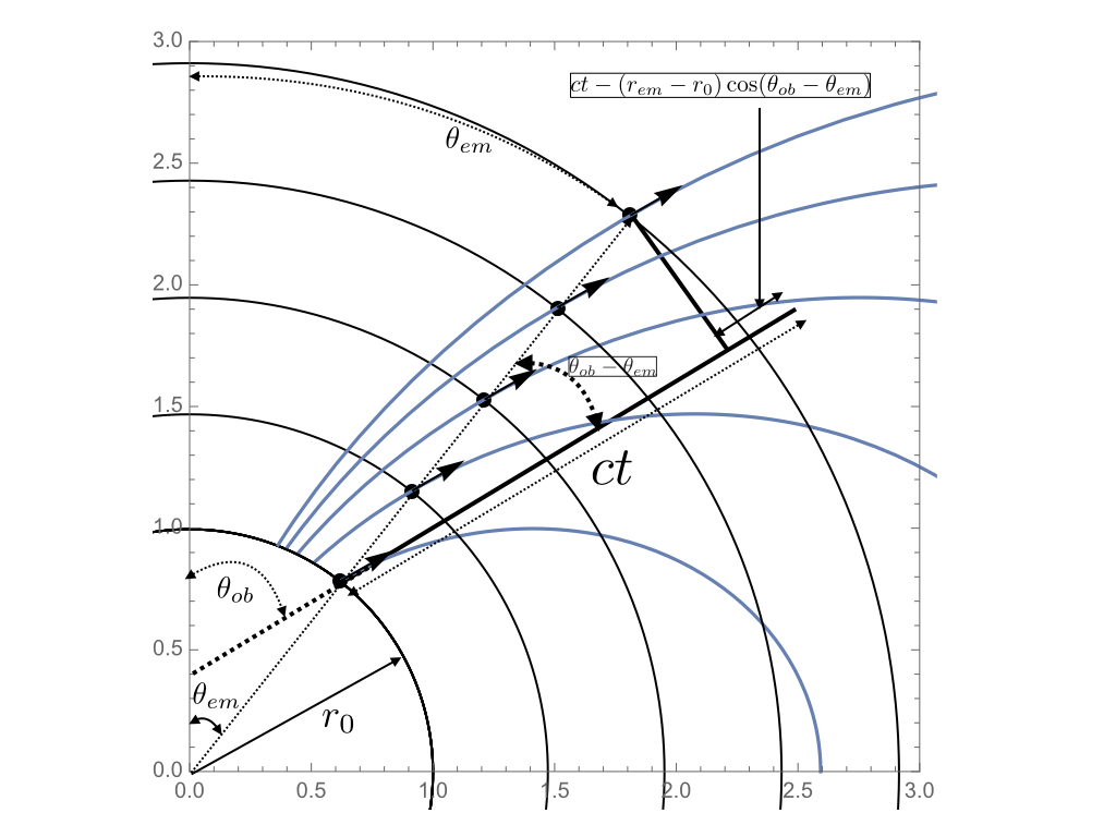
Figure 1: Location of emission points within the magnetosphere. Magnetic axis is vertical. Observer is located at polar angle $\theta_{ob}$, which is time-dependent for the rotating case. At time $t=0$ an emission front is lightened from the surface $r_{0}=1$, propagating along the local magnetic field lines with velocity $\beta$. Circles correspond to the radius $r_{em}$ of the emission points at times $t=0,0.5,1,2$; emission points at each moment are located at radius $r_{em}$ and polar angle $\theta_{em}$; emission is along the local magnetic field. Due to the field lines curvature the emission front at later times lags behind the one emitted at $t=0$ even for $\beta=1$. Observer angle $\theta_{ob}=\pi/4$ in the example pictured. The insert indicates the relation between the observer time and geometrical parameters.

For a field line parametrized by polar angle $\theta_{0}$ at $r_{0}$, a distance along the field line from $\theta_{0}$ to $\theta>\theta_{0}$ is

$$\Delta s=\frac{r_{0}}{\sin^{2}\theta_{0}}\int_{\theta_{0}}^{\theta}\sqrt{1+3\cos^{2}\theta}\sin\theta d\theta$$ (3)

Emitting particles move according to

$$\Delta s=\beta t$$ (4)

where $t$ is the coordinate time.

The points $\theta_{em}$ in the dipolar magnetosphere that have magnetic field along the line of sight satisfy

$$\cos 2\theta_{em}=\frac{1}{6}\left(\sqrt{2}\cos\theta_{ob}\sqrt{\cos\left(2\theta_{ob}\right)+17}+\cos\left(2\theta_{ob}\right)-1\right)$$ (5)

As figure 1 demonstrates, the observer time is given by (speed of light is set to unity)

$$t_{ob}=t-(r_{em}-r_{0})\cos\left(\theta_{ob}-\theta_{em}\right)$$ (6)

with $r_{em}(t)$ given by the requirement that particles propagating along the curved field with velocity $\beta$ emit along the local magnetic field. For nearly straight field lines and highly relativistic velocity, $\beta\approx 1-1/(2\Gamma^{2})$, the effects of field line curvature dominate for $\theta_{ob}-\theta_{em}\geq 1/\Gamma$. (In calculations below the time is normalized to unites $r_{0}/c$, where $r_{0}$ is some initial radius, not necessarily the neutron star radius.)

We then implement the following procedure, Fig. 1

• Given is the observer angle $\theta_{ob}$ (with respect to the magnetic dipole).

• Find the polar angle of the footprint $\theta_{0}^{(0)}$ by solving Eq. (5) and setting $\theta_{em}=\theta_{0}^{(0)}$. (Superscript ⁽⁰⁾ indicates the moment $t=0$.

• After time $t$ the emission front moved along the field lines according to Eqns (3-4), where $\theta_{0}(t)$ is a parameter for the field line emitting at time $t$ (at $t=0$ we have $\theta_{0}(0)=\theta_{0}^{(0)}$)

• For $t\geq 0$, using Eqns. (3-4-5) with $\theta=\theta_{em}$ , find the polar angle of the foot-point $\theta_{0}$, (5), where magnetic field is along the line of sight at time $t$.

• Using (4) find $\theta_{0}$ - the polar angle of the field line that produces emission at time $t$.

• Given time $t$ and the location of the emission point we can calculate the observer time, Eq. (6).

• We then find dependence of $r_{em}$ versus $t_{ob}$.

• Assuming some $\omega(r_{em})$ we find the radius-to-frequency mapping $\omega(t_{ob})$.

Thus, we take into account relativistic transformations and curvature of the field lines in calculating the relations between the observer time versus the coordinate time. We implicitly assume that emitted frequency is the function of the emission radius, $\omega(r_{em})$, but given our uncertainty about the emission properties we do not specify a particulate dependence $\omega(r_{em})$. We plot curves for generic profiles $\omega\propto r_{em}^{-1}$ and $\omega\propto r_{em}^{-3}$; the last scaling is expected if the emission is linearly related to the local magnetic field.

The velocity of the emitting front has a complicated effect on the overall duration of the observed pulse and a range of emitted frequencies. For sub-relativistic velocities $\Delta r_{em}\sim\beta\Delta t$ and $t_{ob}\sim\Delta t$. As $\beta\rightarrow 1$, the observed duration shortens, $t_{ob}\ll\Delta t$. But for sufficiently high velocity, $\beta\approx 1$ with $\theta_{em}-\theta_{ob}\geq 1/\Gamma$, this relativistic line-of-sight contraction become unimportant, as the observed duration is determined by the curvature of field lines.

2.2 Results: stationary magnetosphere

In Fig. 2 we implement the above-describe procedure showing $r_{em}(t_{ob})$ for the extreme relativistic limit of $\beta=1$. The figure demonstrates that the effects of magnetic field line curvature can dominate over the relativistic effects along the line of sight.

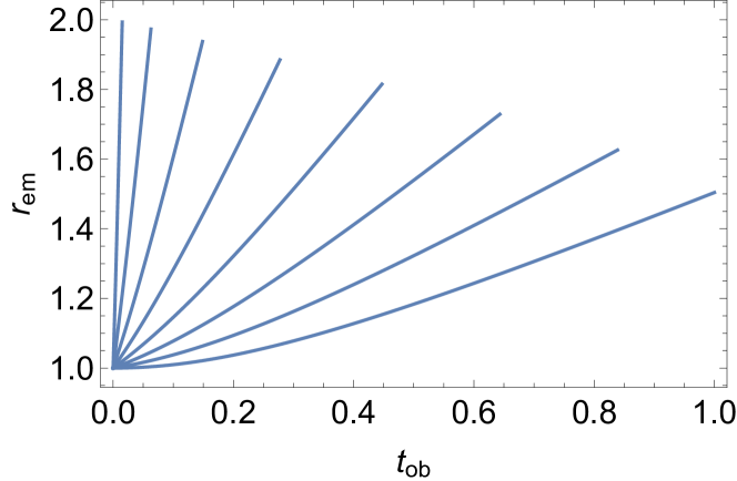
Figure 2: Emission radius as a function of the observer time for different viewing angles, $\theta_{ob}=\pi/8,\,\pi/4...\pi$; non-rotating magnetosphere; $\beta=1$, duration of propagation in coordinate time is $\Delta t=1$. At larger viewing angles the field lines are more curved - this cancels the relativistic line-of-sight effects, producing longer duration pulses even for $\beta=1$. (For $\beta=1$ and $\theta_{ob}=0$ all emission arrives at $t_{ob}=0$). For angles $\theta_{ob}>\pi/2$ it is assumed that only “upper” half of the magnetosphere emits.

For assumed scaling $\omega(r_{em})$ $\omega\propto r_{em}^{-1}$ and $\omega\propto r_{em}^{-3}$ the corresponding curves $\omega(t_{ob})$ are given in Fig. 3. The model generally reproduces, approximately linear drifts rates (see, eg Josephy et al., 2019, Fig. 6) regardless of the particular power law dependence $\omega(r_{em})$. We consider this as a major success of the model.

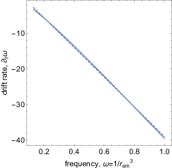
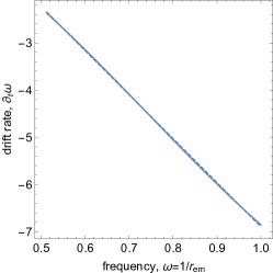
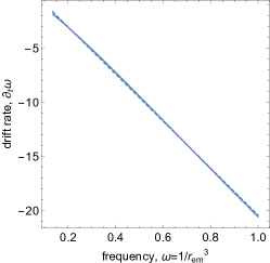
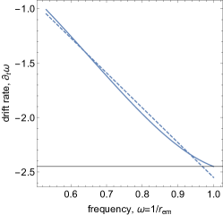
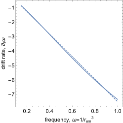
Figure 3: Drift rates in a stationary magnetosphere as function of frequency for two scalings: $\omega\propto r_{em}^{-1}$ (left panels) and $\omega\propto r_{em}^{-3}$ (right panels). Non-Rotating magnetospheres. Top row: $\theta_{ob}=\pi/4$, middle row $\theta_{ob}=\pi/3$, bottom row $\theta_{ob}=\pi/2$. Dashed lines are linear fits $\dot{\omega}\propto\omega$. This simplest case demonstrates that for most observer angles the frequency drift is linear in time (for smaller $\theta_{ob}$ the drift is more linear since the fields lines are straighter near the magnetic pole.

2.3 Rotating magnetosphere

Assume next that the star is rotating with spin frequency $\Omega$. The magnetic polar angle of the line of sight at time $t$ in the pulsar frame is then

$$\cos\theta_{ob}=\cos\alpha\cos\theta_{ob}^{(0)}+\sin\alpha\sin\theta_{ob}^{(0)}\cos(\Delta\phi+t\Omega)$$ (7)

where $\alpha$ is the inclination angle between rotational axis and magnetic moment, $\theta_{ob}^{(0)}$ is the observer angle in the plane comprising vectors of $\Omega$, $\mu$ and the line of sight, and $\Delta\phi$ is the azimuthal angle of the observer with respect to the $\Omega$-$\mu$ plane when the injection starts - this is the phase at $t=0$. (For example, if emission starts when the line of sight is in the $\Omega$-$\mu$ plane, at that moment $\theta_{ob}=\alpha-\theta_{ob}^{(0)}$.)

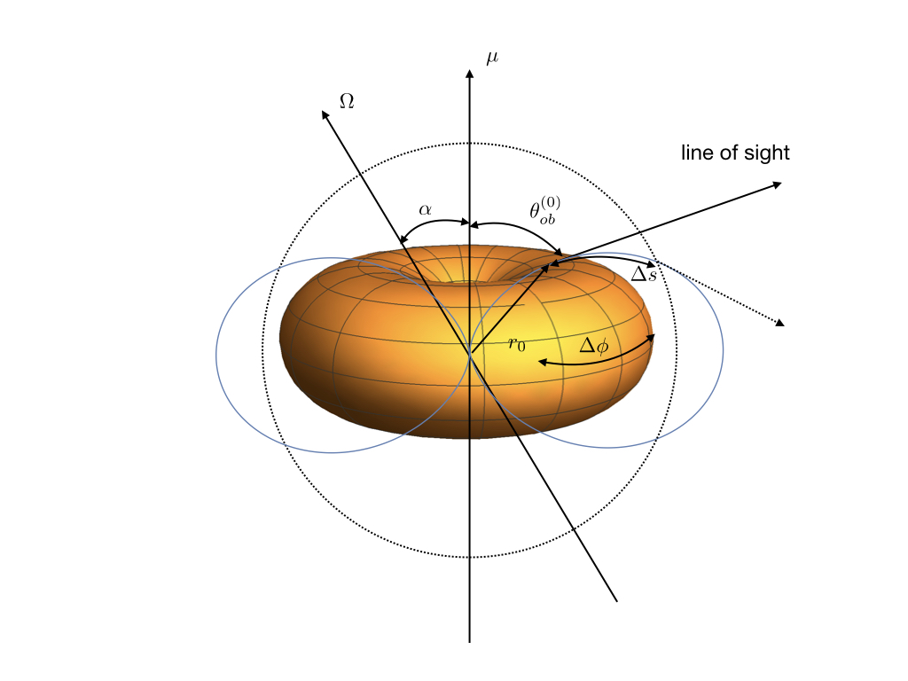
Figure 4: Geometry of the problem at the moment when the line of sight is in the $\mu-\Omega$ plane; reference frame associated with the neutron star. Magnetic moment is inclined by the angle $\alpha$ with respect to the rotation axis $\Omega$. When the line of sight is in the $\mu-\Omega$ plane, the angle between the line of sight and magnetic moment is $\theta_{ob}^{(0)}$. Emission starts at $r_{0}$ (at the moment defined by $\Delta\phi$ and propagates along the local magnetic field according to $\Delta s=\beta t$. Emission is along the local magnetic field. Later times are denoted by dotted lines. The model is inherently 3D - this picture only illustrate the main geometrical factors.

We then implement the procedure, outlined in §2, with the following modifications, see Fig. 4

• Given are the $\theta_{ob}^{(0)}$, $\alpha$, $\beta$, $\Omega$ and $\Delta\phi$

• For $t\geq 0$ implement procedure of §2 with time-dependent $\theta_{ob}$ given by Eq. (7)

2.3.1 Frequency drifts in rotating magnetosphere

In the rotating magnetospheres the observed frequency drifts are generally more complicated, as the line of sight samples larger part of the magnetosphere. A key limitation in the approach is that we assume that the whole surface $r=0$ produced as emission front - thus different parts of the emission front maybe casually disconnected - under certain circumstances this leads to unphysical results (e.g. upward frequency drifts).

In Fig. 5 we plot emission radius as function fo observer time for different pulsar spins. It is clear that for a given intrinsic burst duration larger $\Omega$ produce emission that is seen for longer observer time. This is due to the fact that the line of sight samples larger angular range and correspondingly larger differences in the line of sight advances of the emitting region.

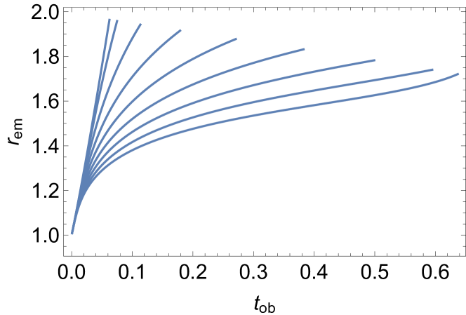
Figure 5: Emission radius as function of the observer time for different $\Omega=0,\pi/8...\pi$ (left to right, $\alpha=\pi/4$, $\delta\phi=0$, $\theta_{ob}=\pi/2$). This plot demonstrates that faster spin increases the observed duration of a pulse, as the line of sight samples larger parameter space.

In Fig. 6 we show the corresponding frequency drifts for selected parameters. As is clear from the plots, the evolution of the peak frequency can be more complicated in the rotation magnetospheres, as the line of sight samples large variations of plasma parameters. (The dimensionless spin $\Omega=\pi/2$ in Fig. 6 is relatively high; smaller $\Omega$ produce more linear scalings)

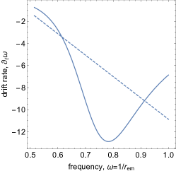
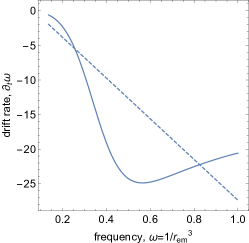
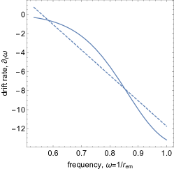
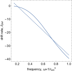
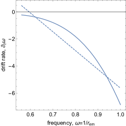
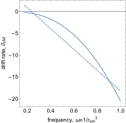
Figure 6: Drift rates as function of frequency in rotating magnetospheres; $\omega\propto r_{em}^{-1}$ (left panels) and $\omega\propto r_{em}^{-3}$ (right panels). Parameters are: $\alpha=\pi/4$, $\theta_{ob}^{(0)}=\pi/2$, $\Omega=\pi 2/$. Top row: $\Delta\phi=-\pi/4$, middle row: $\Delta\phi=0$, bottom row: $\Delta\phi=-\pi/4$. Dashed lines are linear fits. At intermediate frequencies the drifts rate are highly dependent on the spin frequencies, while at higher frequencies the curves converge and hence less sensitivity to spin. This example shows that the model can produce/predicts a variety of frequency drifts.

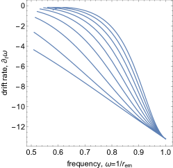
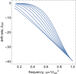
Figure 7: Drift rates as function of frequency in rotating magnetospheres; $\omega\propto r_{em}^{-1}$ (left panel) and $\omega\propto r_{em}^{-3}$ (right panel). Parameters are: $\alpha=\pi/4$, $\theta_{ob}^{(0)}=\pi/2$, $\Delta\phi=0$. Different curves correspond to different spin frequencies $\Omega=0,\,\pi/8...\pi$ (bottom to top). Thus, the rotation of a neutron star does affect the frequency drifts. Closer to $r_{0}$ (higher frequencies) higher spins result in large frequency drifts.

Importantly, depending on the trigger phase $\Delta\phi$ the same object will produce different $r_{em}(t_{ob})$ curves, Fig. 8. This explains why in the Repeaters FRB 121102 different burst have different drifts (Hessels et al., 2019). The fact that different parts of the magnetar magnetosphere can become active also explains the lack of periodicity in repeating FRBs.

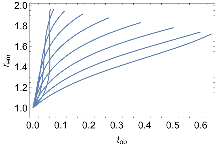
Figure 8: Curves $r_{em}(t_{ob})$ for different launching phases o $\Delta\phi=-\pi/2--\pi/2$ in steps of $\pi/8$ ( $\alpha=\pi/4$, $\theta_{ob}^{(0)}=\pi/2$, $\Omega=\pi/2$. This demonstrates that different behavior can be seen from the same object depending on the initiation moment of the emission front.

2.3.2 Prediction: polarization swings

Polarization behavior of FBRs is, arguably, the most confusing overall (Masui et al., 2015; Petroff et al., 2015; Caleb et al., 2019; Petroff et al., 2019). We are not interested here in the propagation effects (e.g.sometimes huge and sometimes not RM measure). There is a clear, repeated detection of linear polarization. Importantly, FRBs have thus far not shown large polarization angle swings (Petroff et al., 2019).

The present model does not address the origin of polarization, as it would depend on the particular coherent emission mechanism. On basic grounds, polarization is likely to be determined by the local magnetic field within the magnetosphere. The model then does predict polarization angle swings. In the rotating vector model (RVM, Radhakrishnan & Cooke, 1969) polarization swings reflect a local direction of the magnetic field at the emission point. In our notations the position angle of polarization $\chi$ is given by

$$\tan\chi=\frac{\sin\theta_{{ob}}^{(0)}\sin(\Omega t+\Delta\phi)}{\cos\alpha\sin\theta_{{ob}}^{(0)}\cos(\Omega t+\Delta\phi)-\sin\alpha\cos\theta_{{ob}}^{(0)}}$$ (8)

Generally, we do expect polarization swings through the pulse, Fig. 9. Qualitatively, the fastest rate of change of the position angle occurs when the line of sight passes close to the magnetic axis; this requires $\alpha\approx\theta_{{ob}}^{(0)}$ (so that the denominator comes close to zero). This is the case for rotationally powered pulsars. If emission is generated far from the magnetic axis, the expected PA swings are smaller. Thus, we do predict that PA swings will be observed within the pulses, but with values smaller than the ones seen in radio pulsars.

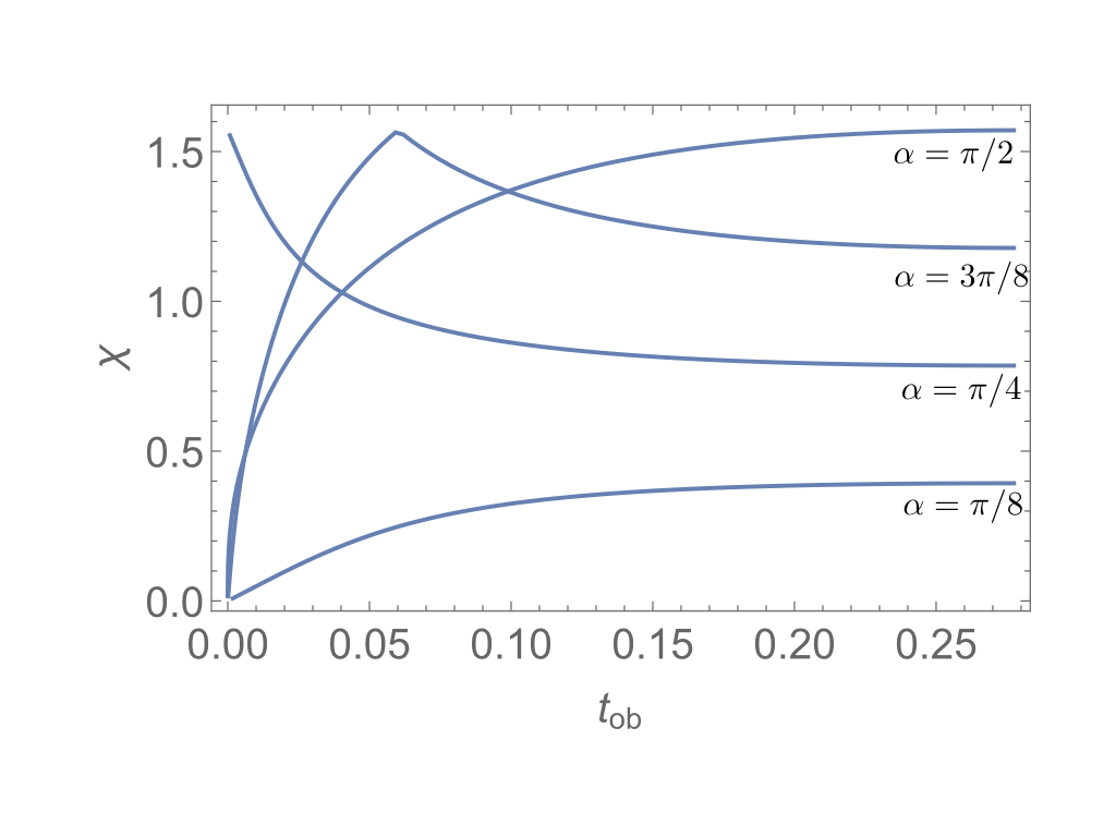
Figure 9: Position angle $\chi$ as function ob the observer time $t_{ob}$ for different $\alpha=0,...\pi/2$ in steps of $\pi/8$; $\Delta\phi=0$, $\Omega=\pi/2$, $\theta_{ob}^{(0)}=\pi/2$.

3 Discussion

In this paper we further argue that frequency drifts observed in FRBs point to the magnetospheres of neutron stars as the origin (see also Lyutikov, 2019b). Our preferred model is a young magnetar-type pulsar producing reconnection events during magnetic relaxation in the magnetospheres (Popov & Postnov, 2013). This should be a special type of magnetars, as there are observational constraints against radio bursts associated with the known magnetars (see, e.g. discussion in Lyutikov, 2019b)

In astronomical setting, the repeater FRB 121102 is localized to an active star-forming galaxy, where ones does naturally expects young neutron stars (Tendulkar et al., 2017). In contrast, FRB 180924 is identified with galaxy dominated by an old stellar population with low star formation rate (Bannister et al., 2019). One possibility is the formation of a neutron star from an accretion induced collapse of a white dwarf with a formation of a neutron star; this process is probably responsible for formation of young pulsars in globular clusters (Lyne et al., 1996).

The main points of the work are:

• The observed drift rate (1) implies sizes of the order of magnetospheres of neutron stars. This is a somewhat independent constraint on the emission size, in addition to total duration of FRBs (which also is consistent with magnetospheric size).

• The observed linear scaling of drift rate with frequency, Eq. (1), is a natural consequence of radius-to-frequency mapping in magnetospheres of neutron stars. It is valid, generally, for any power-law type $\omega(r_{em})$ dependence. In fast rotating pulsars the drifts can have more complicated structure, e.g. Fig. 7.

• Non-observation of drifts in slowly rotating regular magnetars (during radio bursts Maan et al., 2019) is possibly due to the fact that higher spins may lead to higher drift rate, Fig. 7, higher amplitudes, Fig. 2, and longer observer duration, Fig. 5.

• In each given (repeating) FRB emission can originate at arbitrary rotational phases, resulting in different drift profiles in different pulses from a given repeater, Fig. 8.

The model has a number of predictions.

• Polarization swings within the bursts, reminiscent of RVM for pulsars, can be observed. The amplitude of the swings in FRBs is expected to be smaller than in radio pulsar since the emission sights are not limited to the region near the magnetic axis, where PA swings are the largest.

• For some parameters (line of sight, magnetic inclination and spin) the frequency drifts are not linear in frequency, e.g. Fig. 7. Given a limited signal to noise ratio of the typical data, regular, continuous frequency drifts are easier identifiable; more complicated ones are more difficult to find during the de-dispersion procedure. We encourage searchers for more complicated frequency drifts within FRBs.

References

- Bannister et al. (2019) Bannister, K. W., Deller, A. T., Phillips, C., Macquart, J. P., Prochaska, J. X., Tejos, N., Ryder, S. D., Sadler, E. M., Shannon, R. M., Simha, S., Day, C. K., McQuinn, M., North-Hickey, F. O., Bhandari, S., Arcus, W. R., Bennert, V. N., Burchett, J., Bouwhuis, M., Dodson, R., Ekers, R. D., Farah, W., Flynn, C., James, C. W., Kerr, M., Lenc, E., Mahony, E. K., O’Meara, J., Osłowski, S., Qiu, H., Treu, T., U, V., Bateman, T. J., Bock, D. C. J., Bolton, R. J., Brown, A., Bunton, J. D., Chippendale, A. P., Cooray, F. R., Cornwell, T., Gupta, N., Hayman, D. B., Kesteven, M., Koribalski, B. S., MacLeod, A., McClure-Griffiths, N. M., Neuhold, S., Norris, R. P., Pilawa, M. A., Qiao, R. Y., Reynolds, J., Roxby, D. N., Shimwell, T. W., Voronkov, M. A., & Wilson, C. D. 2019, Science, 365, 565
- Caleb et al. (2019) Caleb, M., van Straten, W., Keane, E. F., Jameson, A., Bailes, M., Barr, E. D., Flynn, C., Ilie, C. D., Petroff, E., Rogers, A., Stappers, B. W., Venkatraman Krishnan, V., & Weltevrede, P. 2019, MNRAS, 487, 1191
- Cordes & Chatterjee (2019) Cordes, J. M., & Chatterjee, S. 2019, arXiv e-prints, arXiv:1906.05878
- Hessels et al. (2019) Hessels, J. W. T., Spitler, L. G., Seymour, A. D., Cordes, J. M., Michilli, D., Lynch, R. S., Gourdji, K., Archibald, A. M., Bassa, C. G., Bower, G. C., Chatterjee, S., Connor, L., Crawford, F., Deneva, J. S., Gajjar, V., Kaspi, V. M., Keimpema, A., Law, C. J., Marcote, B., McLaughlin, M. A., Paragi, Z., Petroff, E., Ransom, S. M., Scholz, P., Stappers, B. W., & Tendulkar, S. P. 2019, ApJ, 876, L23
- Josephy et al. (2019) Josephy, A., Chawla, P., Fonseca, E., Ng, C., Patel, C., Pleunis, Z., Scholz, P., Andersen, B. C., Bandura, K., Bhardwaj, M., Boyce, M. M., Boyle, P. J., Brar, C., Cubranic, D., Dobbs, M., Gaensler, B. M., Gill, A., Giri, U., Good, D. C., Halpern, M., Hinshaw, G., Kaspi, V. M., Landecker, T. L., Lang, D. A., Lin, H. H., Masui, K. W., Mckinven, R., Mena-Parra, J., Merryfield, M., Michilli, D., Milutinovic, N., Naidu, A., Pen, U., Rafiei-Ravand i, M., Rahman, M., Ransom, S. M., Renard, A., Siegel, S. R., Smith, K. M., Stairs, I. H., Tendulkar, S. P., Vanderlinde, K., Yadav, P., & Zwaniga, A. V. 2019, arXiv e-prints, arXiv:1906.11305
- Lorimer et al. (2007) Lorimer, D. R., Bailes, M., McLaughlin, M. A., Narkevic, D. J., & Crawford, F. 2007, Science, 318, 777
- Lyne et al. (1996) Lyne, A. G., Manchester, R. N., & D’Amico, N. 1996, ApJ, 460, L41
- Lyutikov (2002) Lyutikov, M. 2002, ApJ, 580, L65
- Lyutikov (2006) —. 2006, MNRAS, 367, 1594
- Lyutikov (2015) —. 2015, MNRAS, 447, 1407
- Lyutikov (2017) —. 2017, ApJ, 838, L13
- Lyutikov (2019a) —. 2019a, arXiv e-prints, arXiv:1901.03260
- Lyutikov (2019b) —. 2019b, arXiv e-prints, arXiv:1908.07313
- Lyutikov et al. (2016) Lyutikov, M., Burzawa, L., & Popov, S. B. 2016, MNRAS, 462, 941
- Maan et al. (2019) Maan, Y., Joshi, B. C., Surnis, M. P., Bagchi, M., & Manoharan, P. K. 2019, ApJ, 882, L9
- Manchester & Taylor (1977) Manchester, R. N., & Taylor, J. H. 1977, Pulsars
- Masui et al. (2015) Masui, K., Lin, H.-H., Sievers, J., Anderson, C. J., Chang, T.-C., Chen, X., Ganguly, A., Jarvis, M., Kuo, C.-Y., Li, Y.-C., Liao, Y.-W., McLaughlin, M., Pen, U.-L., Peterson, J. B., Roman, A., Timbie, P. T., Voytek, T., & Yadav, J. K. 2015, Nature, 528, 523
- Petroff et al. (2015) Petroff, E., Bailes, M., Barr, E. D., Barsdell, B. R., Bhat, N. D. R., Bian, F., Burke-Spolaor, S., Caleb, M., Champion, D., Chandra, P., Da Costa, G., Delvaux, C., Flynn, C., Gehrels, N., Greiner, J., Jameson, A., Johnston, S., Kasliwal, M. M., Keane, E. F., Keller, S., Kocz, J., Kramer, M., Leloudas, G., Malesani, D., Mulchaey, J. S., Ng, C., Ofek, E. O., Perley, D. A., Possenti, A., Schmidt, B. P., Shen, Y., Stappers, B., Tisserand, P., van Straten, W., & Wolf, C. 2015, MNRAS, 447, 246
- Petroff et al. (2019) Petroff, E., Hessels, J. W. T., & Lorimer, D. R. 2019, A&A Rev., 27, 4
- Phillips (1992) Phillips, J. A. 1992, ApJ, 385, 282
- Piran (2004) Piran, T. 2004, Reviews of Modern Physics, 76, 1143
- Popov & Postnov (2013) Popov, S. B., & Postnov, K. A. 2013, arXiv e-prints, arXiv:1307.4924
- Radhakrishnan & Cooke (1969) Radhakrishnan, V., & Cooke, D. J. 1969, Astrophys. Lett., 3, 225
- Spitler et al. (2016) Spitler, L. G., Scholz, P., Hessels, J. W. T., Bogdanov, S., Brazier, A., Camilo, F., Chatterjee, S., Cordes, J. M., Crawford, F., Deneva, J., Ferdman, R. D., Freire, P. C. C., Kaspi, V. M., Lazarus, P., Lynch, R., Madsen, E. C., McLaughlin, M. A., Patel, C., Ransom, S. M., Seymour, A., Stairs, I. H., Stappers, B. W., van Leeuwen, J., & Zhu, W. W. 2016, Nature, 531, 202
- Tendulkar et al. (2017) Tendulkar, S. P., Bassa, C. G., Cordes, J. M., Bower, G. C., Law, C. J., Chatterjee, S., Adams, E. A. K., Bogdanov, S., Burke-Spolaor, S., Butler, B. J., Demorest, P., Hessels, J. W. T., Kaspi, V. M., Lazio, T. J. W., Maddox, N., Marcote, B., McLaughlin, M. A., Paragi, Z., Ransom, S. M., Scholz, P., Seymour, A., Spitler, L. G., van Langevelde, H. J., & Wharton, R. S. 2017, ApJ, 834, L7
- The CHIME/FRB Collaboration et al. (2019a) The CHIME/FRB Collaboration, :, Andersen, B. C., Band ura, K., Bhardwaj, M., Boubel, P., Boyce, M. M., Boyle, P. J., Brar, C., Cassanelli, T., Chawla, P., Cubranic, D., Deng, M., Dobbs, M., Fandino, M., Fonseca, E., Gaensler, B. M., Gilbert, A. J., Giri, U., Good, D. C., Halpern, M., Höfer, C., Hill, A. S., Hinshaw, G., Josephy, A., Kaspi, V. M., Kothes, R., Landecker, T. L., Lang, D. A., Li, D. Z., Lin, H. H., Masui, K. W., Mena-Parra, J., Merryfield, M., Mckinven, R., Michilli, D., Milutinovic, N., Naidu, A., Newburgh, L. B., Ng, C., Patel, C., Pen, U., Pinsonneault-Marotte, T., Pleunis, Z., Rafiei-Ravandi, M., Rahman, M., Ransom, S. M., Renard, A., Scholz, P., Siegel, S. R., Singh, S., Smith, K. M., Stairs, I. H., Tendulkar, S. P., Tretyakov, I., Vanderlinde, K., Yadav, P., & Zwaniga, A. V. 2019a, arXiv e-prints, arXiv:1908.03507
- The CHIME/FRB Collaboration et al. (2019b) The CHIME/FRB Collaboration, Amiri, M., Bandura, K., Bhardwaj, M., Boubel, P., Boyce, M. M., Boyle, P. J., . Brar, C., Burhanpurkar, M., Cassanelli, T., Chawla, P., Cliche, J. F., Cubranic, D., Deng, M., Denman, N., Dobbs, M., Fandino, M., Fonseca, E., Gaensler, B. M., Gilbert, A. J., Gill, A., Giri, U., Good, D. C., Halpern, M., Hanna, D. S., Hill, A. S., Hinshaw, G., Höfer, C., Josephy, A., Kaspi, V. M., Landecker, T. L., Lang, D. A., Lin, H. H., Masui, K. W., Mckinven, R., Mena-Parra, J., Merryfield, M., Michilli, D., Milutinovic, N., Moatti, C., Naidu, A., Newburgh, L. B., Ng, C., Patel, C., Pen, U., Pinsonneault-Marotte, T., Pleunis, Z., Rafiei-Ravandi, M., Rahman, M., Ransom, S. M., Renard, A., Scholz, P., Shaw, J. R., Siegel, S. R., Smith, K. M., Stairs, I. H., Tendulkar, S. P., Tretyakov, I., Vanderlinde, K., & Yadav, P. 2019b, Nature, 566, 235
- Wang et al. (2019) Wang, W., Zhang, B., Chen, X., & Xu, R. 2019, ApJ, 876, L15