Quasinormal modes, echoes and the causal structure of the Green’s function

Lam Hui${}^{\,a}$, Daniel Kabat${}^{\,b}$ and Sam S. C. Wong${}^{\,a,\,c}$

^a Department of Physics, Center for Theoretical Physics, Columbia University,

538 West 120th Street, New York, NY 10027, USA

^b Department of Physics and Astronomy, Lehman College, City University of New York,

250 Bedford Park Blvd. West, Bronx NY 10468, USA

^c Center for Particle Cosmology, Department of Physics and Astronomy,

University of Pennsylvania 209 S. 33rd St., Philadelphia, PA 19104, USA

1 Introduction

Detection of gravitational waves from binary black hole collisions [1] and future precision measurements provide an unprecedented tool for probing gravity in the strong field regime. Tremendous efforts have been made in extracting information from the emitted gravitational waves. The ringdown phase of a black hole collision can be described analytically by linearized gravity around the black hole background [2, 3] . The ringing modes of the merged black hole are known as quasinormal modes (QNMs) and their characteristic frequencies and decay are given by a set of complex quasinormal frequencies (QNFs).

Pioneering work by Regge-Wheeler [4] and by Zerilli [5] established the equations describing the (parity odd and even) linearized metric perturbations around a Schwarzschild black hole. In both cases, the relevant equation, after factoring out suitable angular harmonics, takes the form:

$$(\partial_{t}^{2}-\partial_{x}^{2}+V(x))\phi(t,x)=0\,,$$ (1.1)

where $\phi$ is the perturbation of interest, $x$ represents the (tortoise) radial coordinate and $V(x)$ represents the appropriate potential; the dependence on the angular harmonic number $\ell$ has been suppressed. For perturbations around a Kerr black hole, the relevant equation has an additional term with a single time derivative (Teukolsky [6]), but upon Fourier transforming in time i.e. $\phi\propto e^{-i\omega t}$, the resulting equation is not too different from the above, i.e. $(-\partial_{x}^{2}+\tilde{V})\phi=0$ with the modified $\tilde{V}$ understood to contain dependence on the frequency $\omega$. The excitation and decay of perturbations around Kerr black holes have been studied in [7, 8].

As an example, the Regge-Wheeler potential takes the form: $V=(1-1/r)[\ell(\ell+1)/r^{2}-3/r^{3}]$, with the Schwarzschild radius set to unity, and $r$ and $x$ are related by $x=r+{\,\rm ln\,}(r-1)$. The potential peaks around $|x|$ of order unity, and tapers off as $x\rightarrow-\infty$ (where the horizon is located) and as $x\rightarrow\infty$ (far away from the black hole). It has long been appreciated that the QNM spectrum is sensitive to modifications to $V$ [9, 10], even if such modifications are localized far away from where the Regge-Wheeler potential peaks. A concrete example is the potential generated by the environment around the black hole, such as gas, dark matter and stars [11]. In other words, the QNM spectrum, unlike the bound-state spectra we encounter in quantum mechanics, is altered significantly even by distant modifications to the original potential. Recently, there has been much attention on distant modifications of this kind, but for exotic objects such as wormholes, or objects with some sort of a membrane or firewall just outside the would-be horizon [12, 13, 14, 15, 16, 17, 18, 19]. Such objects effectively have two well-separated potential bumps, one of which is the essentially the Regge-Wheeler potential. One interesting outcome of the ringdown computation for these objects is that despite the vastly different QNM spectrum compared to a normal black hole, the ringdown waveform of the former is remarkably similar to that of the latter (e.g. compare Fig. 2 and Fig. 4 of [12]), except for the presence of echoes over long time scales. Our goal in this paper is to reconcile these two seemingly contradictory facts—significantly different QNM spectra, yet rather similar initial ringdown waveforms. The tool for studying time evolution is the Green’s function. We will explicate the relation between the QNM spectrum and the Green’s function, and introduce an echo expansion which clarifies the causal structure of the latter. We will use the simple example of a potential with two separated delta functions to illustrate the main ideas.

It should be emphasized that much of the discussion here is not new. The relation between the QNM spectrum and poles of the Green’s function was discussed for instance in [20, 21, 22, 23]. An expansion of the Green’s function in terms of echoes can be found in [18, 24, 25]. The use of two disjoint delta functions, or more general disjoint bumps, as a model potential to illustrate properties of the QNM can be found in [24, 26, 27, 28, 25]. Our goal here is a modest one: to clarify under what conditions the real time evolution of some localized perturbations is sensitive (or insensitive) to the full QNM spectrum. Related ideas were discussed by [29].

An outline of this paper is as follows. In section 2 we present a few simple results for $\delta$-function potentials to motivate the rest of our analysis. In section 3 we give a general discussion of Green’s functions, quasinormal modes and echoes for a pair of potentials with disjoint bounded support. In section 4 we use the soluble example of $\delta$-function potentials to illustrate more general phenomena. In section 5 we study generic potentials of finite width in more detail and show that the echoes respect causality. We conclude in section 6, where we also discuss under what conditions a small change to the potential produces a small change to the Green’s function. The appendices contain some supporting material: a review of Green’s function solutions to the wave equation (appendix A), an alternate derivation of the Green’s function for a potential consisting of multiple $\delta$-functions (appendix B), and a WKB analysis of the matching coefficients for a general potential (appendix C).

2 Motivation

Quasinormal modes describe the return to equilibrium of a perturbed field. They are defined by “radiative” boundary conditions which are purely outgoing at future null infinity (and purely ingoing at any future horizons). But as globally-defined quantities, quasinormal modes can be very sensitive to the global structure of a spacetime. Even small perturbations at large distances can dramatically change the spectrum of quasinormal modes.

As a simple example, consider the wave equation in 1+1 dimensions with a $\delta$-function potential:

$$\left(\partial_{t}^{2}-\partial_{x}^{2}+V_{0}\delta(x)\right)\phi(t,x)=0\,.$$ (2.1)

Here $V_{0}$ is a constant which we take to be positive, corresponding to a repulsive potential, similar to what one encounters in the case of the black hole. This wave equation has a unique solution with quasinormal boundary conditions:

$$\phi(t,x)={\rm const.}\,e^{-{1\over 2}V_{0}(t-|x|)}\,.$$ (2.2)

The mode decays with time and we can read off the unique quasinormal frequency $\omega=-{i\over 2}V_{0}$ (our frequency convention is $\phi\propto e^{-i\omega t}$). It obeys the appropriate quasinormal boundary conditions at future null infinity, namely that $\phi$ is right-moving (a function of $t-x$) as $t,x\rightarrow+\infty$ and left-moving (a function of $t+x$) as $t\rightarrow+\infty$, $x\rightarrow-\infty$. But the mode grows exponentially at spatial infinity, which suggests that it is very sensitive to distant perturbations.

To see that this is indeed the case, let’s compare this to the wave equation with a pair of $\delta$-function potentials:

$$\left(\partial_{t}^{2}-\partial_{x}^{2}+V_{1}\delta(x)+V_{2}\delta(x-L)\right)\phi(t,x)=0\,.$$ (2.3)

We will work out the quasinormal spectrum for this problem in section 4. The result is shown in Fig. 1, where we have plotted the quasinormal frequencies in terms of the Laplace transform variable $s=-i\omega$. The single mode with $s=-V_{0}/2$ splits into the infinite tower of modes shown in the figure. Note that the real part of $s$ is always negative for the QNM, corresponding to a decay with time i.e. $e^{-i\omega t}=e^{st}$.

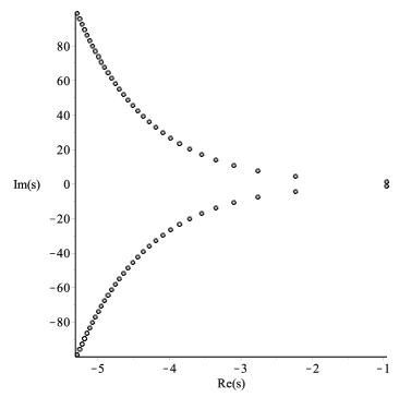
Figure 1: The quasinormal spectrum for a pair of $\delta$-functions with $V_{1}=V_{2}=L=1$, obtained by setting the Wronskian (4.11) to zero. We show modes with $-100<{\rm Im}\,s<100$.

This dramatic change has a simple interpretation, that it captures the multiple reflections (echoes) which are present in the two-$\delta$-function system. These echoes, illustrated in Fig. 2, dramatically change the late-time behavior of the field.

Figure 2: A solution to the double $\delta$-function potential, obtained using the exact Green’s function (4), for $V_{1}=23,\,V_{2}=11$ and $L=1$. Initial conditions: $\phi(0,x)=0$, $\partial_{t}\phi(0,x)=500(2-x)e^{-20(x-2)^{2}}$. The color coding reflects the value of $\phi$ as indicated on the side bar.

The purpose of this paper is to put these statements on a firm footing, using the language of the retarded Green’s function, in the context of two disjoint potentials with bounded support. The restriction to bounded support is for mathematical convenience, as it will enable us to make sharp statements about the causality properties of the echo expansion in section 5. A discussion of late-time behavior for potentials with more general asymptotic behavior can be found in [30, 31].

3 Green’s function and quasinormal modes—general results and application to disjoint potentials

In this section we begin with a general discussion of the Green’s function and quasinormal modes in $1+1$ dimensions, then specialize to two potentials with disjoint bounded support.

We are interested in the retarded Green’s function which satisfies

$$\left(\partial_{t}^{2}-\partial_{x}^{2}+V(x)\right)G(t,x|t^{\prime},x^{\prime})=\delta(t-t^{\prime})\delta(x-x^{\prime})$$ (3.1)

$$G=0\qquad\hbox{\rm if $t<t^{\prime}$}$$ (3.2)

The Green’s function only depends on $t-t^{\prime}$, so a Laplace transform

$$G(s;x|x^{\prime})=\int_{0^{-}}^{\infty}dt\,e^{-st}G(t,x|0,x^{\prime})$$ (3.3)

leads to

$$\left(-\partial_{x}^{2}+s^{2}+V(x)\right)G(s;x|x^{\prime})=\delta(x-x^{\prime})$$ (3.4)

Then we can invert to find

$$G(t,x|t^{\prime},x^{\prime})=\int_{c-i\infty}^{c+i\infty}{ds\over 2\pi i}e^{s(t-t^{\prime})}G(s;x|x^{\prime})$$ (3.5)

(the contour runs parallel to the ${\rm Im}\,s$ axis, but with a positive real part so that it lies to the right of all singularities). Our choice of Laplace transform is necessary but not sufficient to give a retarded Green’s function, and we still need to ensure that the retarded boundary condition (3.2) is satisfied. Given the inverse transformation (3.5), this amounts to demanding that

$$G(s;x|x^{\prime}) {\rm Re}\,s\rightarrow+\infty$$ is bounded as (3.6)

We still have to build a 1-dimensional Green’s function satisfying (3.4), (3.6). To solve (3.4) suppose we find any two linearly-independent solutions $\phi_{\pm}(x,s)$ to the homogeneous equation

$$\left(-\partial_{x}^{2}+s^{2}+V(x)\right)\phi(s,x)=0$$ (3.7)

Then a 1D Green’s function is [32]

$$G(s;x|x^{\prime})={1\over W}\left(\phi_{-}(s,x)\phi_{+}(s,x^{\prime})\theta(x-x^{\prime})+\phi_{+}(s,x)\phi_{-}(s,x^{\prime})\theta(x^{\prime}-x)\right)\,,$$ (3.8)

where the Wronskian

$$W\equiv W[\phi_{-},\phi_{+}](s)\equiv\phi_{-}\partial_{x}\phi_{+}-\phi_{+}\partial_{x}\phi_{-}$$ (3.9)

is $x$-independent, and $\theta(x-x^{\prime})$ is the step function i.e. it vanishes if $x-x^{\prime}<0$ and equals unity otherwise.

The appropriate choice of $\phi_{-}$ and $\phi_{+}$ is dictated by (3.6). Since we’re considering potentials with bounded support this is simplest to discuss to the left and right of the potential, where the two independent homogeneous solutions are just growing and decaying exponentials. To satisfy (3.6) we take

$$\phi_{+}(s,x)=e^{sx}\qquad\,\,\,x<{\rm min}\,{\rm supp}\,V$$ (3.10)

$$\phi_{-}(s,x)=e^{-sx}\qquad x>{\rm max}\,{\rm supp}\,V\,,$$ (3.11)

Here the support of the potential is

$${\rm supp}\,V=\{x\,:\,V(x)\not=0\}\,.$$ (3.12)

Now suppose the general solution to (3.7) behaves as

$$\phi(s,x)=\left\{\begin{array}[]{ll}\alpha e^{sx}+\beta e^{-sx}&x<{\rm min}\,{\rm supp}\,V\\ \gamma e^{sx}+\delta e^{-sx}&x>{\rm max}\,{\rm supp}\,V\end{array}\right.$$ (3.15)

$$\left(\begin{array}[]{c}\gamma\\ \delta\end{array}\right)=\left(\begin{array}[]{cc}m^{++}&m^{+-}\\ m^{-+}&m^{--}\end{array}\right)\left(\begin{array}[]{c}\alpha\\ \beta\end{array}\right)$$ (3.22)

(the “matching coefficients” $m^{\pm\pm}$ are related to the transmission and reflection coefficients). For instance, $\phi_{+}$ has $\alpha=1$ and $\beta=0$ and thus $\gamma=m^{++}$ and $\delta=m^{-+}$. On the other hand, $\phi_{-}$ has $\gamma=0$ and $\delta=1$, and thus $\alpha=-m^{+-}$ and $\beta=m^{++}$. Since the Wronskian is independent of $x$ we can compute it for $x>{\rm max}\,{\rm supp}\,V$, where $\phi_{+}=m^{++}e^{sx}+m^{-+}e^{-sx}$ and $\phi_{-}=e^{-sx}$ and hence

$$W=2sm^{++}\,,$$ (3.24)

where $m^{++}$ is in general a function of $s$. The Green’s function is then

$$G(t,x|t^{\prime},x^{\prime})=\int_{c-i\infty}^{c+i\infty}{ds\over 2\pi i}e^{s(t-t^{\prime})}{1\over 2sm^{++}}\left(\phi_{-}(s,x)\phi_{+}(s,x^{\prime})\theta(x-x^{\prime})+\phi_{+}(s,x)\phi_{-}(s,x^{\prime})\theta(x^{\prime}-x)\right)\,.$$ (3.25)

When the Wronskian vanishes the solutions $\phi_{+}$ and $\phi_{-}$ are linearly dependent. Recall that $\phi_{+}$ behaves as $e^{sx}$ to the far left, and $\phi_{-}$ behaves as $e^{-sx}$ to the far right; recall also that the time dependence of the $s$ mode is $e^{st}$. To have linearly dependent $\phi_{+}$ and $\phi_{-}$ means there is a single solution which behaves $e^{s(t+x)}$ to the far left and $e^{s(t-x)}$ to the far right. This is precisely a solution that obeys the standard quasinormal boundary conditions (i.e. a solution that is purely outgoing at both boundaries of the domain of interest). So quasinormal frequencies (in Laplace space) are zeroes of the Wronskian [21, 31].

Let us wrap up this general discussion of the Green’s function by noting how it is used to evolve the $\phi$ field. As reviewed in appendix A, for $t>t^{\prime}$ we have

$$\phi(t,x)=\int_{-\infty}^{\infty}dx^{\prime}\left[G(t,x|t^{\prime},x^{\prime})\partial_{t^{\prime}}\phi(t^{\prime},x^{\prime})-\phi(t^{\prime},x^{\prime})\partial_{t^{\prime}}G(t,x|t^{\prime},x^{\prime})\right]\,.$$ (3.26)

Thus, given some localized field configuration and its time derivative at $t^{\prime}$, the Green’s function allows us to evolve the field forward to time $t$. It is perhaps not surprising that such a Green’s function knows about the quasinormal spectrum—the influence from the initial disturbance at $t^{\prime}$ propagates in an outgoing manner towards the far left and far right.

The expressions so far are rather general. Let us specialize to the case where $V(x)$ consists of two pieces with disjoint bounded support:

$$V(x)=V_{1}(x)+V_{2}(x-L)\,.$$ (3.27)

We have in mind that $V_{1}$ and $V_{2}$ are separately supported around their respective origin i.e. $V_{1}(x)$ is non-vanishing around $x=0$, and $V_{2}(x-L)$ is non-vanishing around $x-L=0$. We have introduced $L>0$ as an explicit parameter controlling the separation. It’s straightforward to work out a composition law for the Wronskian. For $x<{\rm min}\,{\rm supp}\,V_{1}$ we should take the solution

$$\phi_{+}(s,x)=e^{sx}\,.$$ (3.28)

Then for ${\rm max}\,{\rm supp}\,V_{1}<x<L+{\rm min}\,{\rm supp}\,V_{2}$ we will have

$$\phi_{+}(s,x) = m_{1}^{++}e^{sx}+m_{1}^{-+}e^{-sx}$$

$$= e^{sL}m_{1}^{++}e^{s(x-L)}+e^{-sL}m_{1}^{-+}e^{-s(x-L)}\,.$$

In this form we can use the matching coefficients for $V_{2}$ to find the behavior for $x>L+{\rm max}\,{\rm supp}\,V_{2}$, namely

$$\phi_{+}(s,x)=\left(m_{2}^{++}m_{1}^{++}+e^{-2sL}m_{2}^{+-}m_{1}^{-+}\right)e^{sx}+\left(m_{2}^{--}m_{1}^{-+}+e^{2sL}m_{2}^{-+}m_{1}^{++}\right)e^{-sx}\,.$$ (3.30)

In this range of $x$ we should take $\phi_{-}(s,x)=e^{-sx}$, so the Wronskian is

$$W_{1+2}=2s\left(m_{2}^{++}m_{1}^{++}+e^{-2sL}m_{2}^{+-}m_{1}^{-+}\right)\,.$$ (3.31)

Equivalently we have a composition law

$$W_{1+2}={1\over 2s}W_{1}W_{2}+2se^{-2sL}m_{2}^{+-}m_{1}^{-+}\,.$$ (3.32)

Note the exponential dependence on $L$. The Green’s function is

$$G(t,x|t^{\prime},x^{\prime}) = \int_{c-i\infty}^{c+i\infty}{ds\over 2\pi i}e^{s(t-t^{\prime})}{1\over 2s\left(m_{2}^{++}m_{1}^{++}+e^{-2sL}m_{2}^{+-}m_{1}^{-+}\right)}$$ (3.33)

$$\qquad\left(\phi_{-}(s,x)\phi_{+}(s,x^{\prime})\theta(x-x^{\prime})+\phi_{+}(s,x)\phi_{-}(s,x^{\prime})\theta(x^{\prime}-x)\right)\,.$$

The question is how to interpret (3.33). Compared to (3.25) the main thing that has changed is the denominator. We propose that this should be expanded in powers of $e^{-sL}$.

$$G(t,x|t^{\prime},x^{\prime}) = \sum_{k=0}^{\infty}(-1)^{k}\int_{c-i\infty}^{c+i\infty}{ds\over 2\pi i}\,{\left(m_{2}^{+-}m_{1}^{-+}\right)^{k}\over 2s\left(m_{2}^{++}m_{1}^{++}\right)^{k+1}}e^{s(t-t^{\prime}-2kL)}$$ (3.34)

$$\qquad\left(\phi_{-}(s,x)\phi_{+}(s,x^{\prime})\theta(x-x^{\prime})+\phi_{+}(s,x)\phi_{-}(s,x^{\prime})\theta(x^{\prime}-x)\right)$$

This can be understood as a sum over echoes: if we ignore a possible exponential $s$ dependence of the matching coefficients $m^{\pm\pm}_{1,2}$, the $k^{th}$ term experiences a time delay of $2kL$. Note that for any fixed $t-t^{\prime}$ the sum over echoes truncates, since for sufficiently large $k$ the contour can be closed to the right and the integral vanishes.

To make the echoes more explicit we can substitute expressions such as (3.28), (3), (3.30) (and their analogs for $\phi_{-}$) into the Green’s function. For example, suppose $x^{\prime}<{\rm min}\,{\rm supp}\,V_{1}$ and $x>L+{\rm max}\,{\rm supp}\,V_{2}$. Then $\phi_{+}(x^{\prime})=e^{sx^{\prime}}$, $\phi_{-}(x)=e^{-sx}$ and

$$G(t,x|t^{\prime},x^{\prime})=\sum_{k=0}^{\infty}(-1)^{k}\int_{c-i\infty}^{c+i\infty}{ds\over 2\pi i}\,{\left(m_{2}^{+-}m_{1}^{-+}\right)^{k}\over 2s\left(m_{2}^{++}m_{1}^{++}\right)^{k+1}}e^{s\big{(}t-t^{\prime}-(x-x^{\prime})-2kL\big{)}}$$ (3.35)

Suppose the matching coefficients $m^{\pm\pm}_{1,2}$ have no exponential $s$ dependence; then the $k^{th}$ term in the sum vanishes if $t-t^{\prime}<x-x^{\prime}+2kL$. This is in accord with the expected time delay for $k$ back-and-forth echoes between sharply-localized potentials separated by a distance $L$. For $\delta$-function potentials this conclusion is accurate as we show in section 4. But for finite-width potentials there are corrections. We analyze these corrections in section 5 where we show in general that the echoes respect causality.

4 $\delta$-function potentials

In this section we analyze $\delta$-function potentials as a tractable example to illustrate the general phenomenon.

We first treat a single $\delta$-function. The wave equation is given in (2.1), which after a Laplace transform becomes

$$\left(-\partial_{x}^{2}+s^{2}+V_{0}\delta(x)\right)\phi(s,x)=0$$ (4.1)

This has a pair of solutions, related by $s\rightarrow-s$, given by

$$\phi(s,x)=e^{sx}+{V_{0}\over s}\sinh(sx)\theta(x)$$ (4.2)

$$\phi(s,x)=e^{-sx}+{V_{0}\over s}\sinh(sx)\theta(x)$$ (4.3)

Comparing to (3.15) we read off the matching coefficients

$$\begin{array}[]{ll}m^{++}=1+{V_{0}\over 2s}&\quad m^{-+}=-{V_{0}\over 2s}\\ m^{+-}={V_{0}\over 2s}&\quad m^{--}=1-{V_{0}\over 2s}\end{array}$$ (4.4)

From (3.24) the Wronskian is

$$W=2sm^{++}=2s+V_{0}$$ (4.5)

and the Green’s function is

$$G(t,x|t^{\prime},x^{\prime})=\int_{c-i\infty}^{c+i\infty}{ds\over 2\pi i}\,{1\over 2s+V_{0}}e^{s(t-t^{\prime})}\left(\phi_{-}(s,x)\phi_{+}(s,x^{\prime})\theta(x-x^{\prime})+\phi_{+}(s,x)\phi_{-}(s,x^{\prime})\theta(x^{\prime}-x)\right)$$ (4.6)

Here solutions $\phi_{\pm}$ with the behavior (3.10), (3.11) are given by

$$\phi_{+}(s,x)=e^{sx}+{V_{0}\over s}\sinh(sx)\theta(x)$$ (4.7)

$$\phi_{-}(s,x)=e^{-sx}-{V_{0}\over s}\sinh(sx)\theta(-x)$$ (4.8)

As expected the Wronskian (4.5) has a zero at the quasinormal frequency $s=-V_{0}/2$. The contour integral (4.6) gives

$$G(t,x|t^{\prime},x^{\prime})=\left\{\begin{array}[]{ll}0&\quad t-t^{\prime}<|x-x^{\prime}|\\ {1\over 2}&\quad|x-x^{\prime}|<t-t^{\prime}<|x|+|x^{\prime}|\\ {1\over 2}\exp\left(-{1\over 2}V_{0}(t-t^{\prime}-|x|-|x^{\prime}|)\right)&\quad t-t^{\prime}>|x|+|x^{\prime}|\end{array}\right.$$ (4.9)

or alternatively

$$G(t,x|t^{\prime},x^{\prime})={1\over 2}\theta(t-t^{\prime}-|x-x^{\prime}|)+{1\over 2}\left(e^{-{1\over 2}V_{0}(t-t^{\prime}-|x|-|x^{\prime}|)}-1\right)\theta(t-t^{\prime}-|x|-|x^{\prime}|)$$ (4.10)

The first line of (4.9) shows that the Green’s function vanishes unless $(t,x)$ lies in the causal future of $(t^{\prime},x^{\prime})$. The second line recovers the Green’s function without a potential, in the case where causal curves from $(t^{\prime},x^{\prime})$ to $(t,x)$ do not touch $x=0$. In the last line – the regime where scattering off the potential is permitted by causality – the Green’s function depends on $V_{0}$.

To extend this to the pair of $\delta$-functions (2.3) we make use of (3.31), which tells us that the Wronskian for the combined system is (recall $L>0$)

$$W={1\over 2s}\left[\left(2s+V_{1}\right)\left(2s+V_{2}\right)-V_{1}V_{2}e^{-2sL}\right]$$ (4.11)

Zeroes of the Wronskian determine quasinormal frequencies (the dictionary is $\omega=is$). The individual potentials had zeroes at $s=-V_{1}/2$ and $s=-V_{2}/2$, but the combined system has an infinite number of quasinormal frequencies. This is illustrated in Fig. 1 for the case $V_{1}=V_{2}=L=1$.

The Green’s function for the combined system is given by (3.33),

$$G(t,x|t^{\prime},x^{\prime}) = \int_{c-i\infty}^{c+i\infty}{ds\over 2\pi i}e^{s(t-t^{\prime})}{2s\over\left(2s+V_{1}\right)\left(2s+V_{2}\right)-V_{1}V_{2}e^{-2sL}}$$ (4.12)

$$\qquad\left(\phi_{-}(s,x)\phi_{+}(s,x^{\prime})\theta(x-x^{\prime})+\phi_{+}(s,x)\phi_{-}(s,x^{\prime})\theta(x^{\prime}-x)\right)\,,$$

where solutions $\phi_{\pm}$ satisfying (3.10), (3.11) are

$$\phi_{+}(s,x)=e^{sx}+{V_{1}\over s}\sinh(sx)\theta(x)+{V_{2}\over s}\Big{(}e^{sL}+{V_{1}\over s}\sinh(sL)\Big{)}\sinh\big{(}s(x-L)\big{)}\theta(x-L)$$ (4.13)

$$\phi_{-}(s,x)=e^{-sx}-{V_{2}\over s}e^{-sL}\sinh\big{(}s(x-L)\big{)}\theta(L-x)-{V_{1}\over s}\Big{(}1+{V_{2}\over s}e^{-sL}\sinh(sL)\Big{)}\sinh(sx)\theta(-x)\,.$$

This leads to

$$G(t,x|t^{\prime},x^{\prime}) =\int_{c-i\infty}^{c+i\infty}{ds\over 2\pi i}e^{s(t-t^{\prime})}\Bigg{[}\frac{1}{2s}e^{-s|x-x^{\prime}|}$$

$$\quad+\frac{V_{1}(2s+V_{2})e^{-s(|x|+|x^{\prime}|)}-V_{1}V_{2}e^{-s(|x|+L+|L-x^{\prime}|)}}{2s\left[V_{1}V_{2}e^{-2sL}-(2s+V_{1})(2s+V_{2})\right]}$$

$$\quad+\frac{V_{2}(2s+V_{1})e^{-s(|L-x|+|L-x^{\prime}|)}-V_{1}V_{2}e^{-s(|L-x|+L+|x^{\prime}|)}}{2s\left[V_{1}V_{2}e^{-2sL}-(2s+V_{1})(2s+V_{2})\right]}\Bigg{]}\,.$$ (4.14)

An alternate derivation of this result can be found in appendix B.

As we now show, this can be interpreted in terms of echoes by expanding in powers of $e^{-sL}$. The inverse Laplace transform in the first line just gives the usual Green’s function for the operator $\partial_{t}^{2}-\partial_{x}^{2}$.

$${\cal L}^{-1}\left[\frac{1}{2s}e^{-s|x-x^{\prime}|}\right]=\frac{1}{2}\theta(t-t^{\prime}-|x-x^{\prime}|)$$ (4.15)

The second and third lines are sensitive to the potential and have poles at the quasinormal frequencies. Let’s focus on the first term in the second line,

$$\frac{V_{1}(2s+V_{2})e^{-s(|x|+|x^{\prime}|)}}{2s\left[V_{1}V_{2}e^{-2sL}-(2s+V_{1})(2s+V_{2})\right]}$$

$$=\; -\sum_{k=0}^{\infty}\frac{e^{-s(2kL+|x|+|x^{\prime}|)}}{2s\left(s+\frac{V_{2}}{2}\right)^{k}\left(s+\frac{V_{1}}{2}\right)^{k+1}}\left(\frac{V_{2}}{2}\right)^{k}\left(\frac{V_{1}}{2}\right)^{k+1}$$ (4.16)

where we have expanded in $e^{-2sL}$. Now the poles are of finite order and can be inverse Laplace transformed.

$${\cal L}^{-1}[\cdots]=\; \frac{1}{2}\left(e^{-\frac{V_{1}}{2}(t-t^{\prime}-|x|-|x^{\prime}|)}-1\right)\theta(t-t^{\prime}-|x|-|x^{\prime}|)$$

$$-\sum_{k=1}^{\infty}\frac{1}{2}\Bigg{[}\frac{1}{k!}\frac{d^{k}}{ds^{k}}\left.\left(\frac{e^{s(t-t^{\prime}-2kL-|x|-|x^{\prime}|)}}{s\left(s+\frac{V_{2}}{2}\right)^{k}}\right)\right|_{s=-\frac{V_{1}}{2}}\left(\frac{V_{2}}{2}\right)^{k}\left(\frac{V_{1}}{2}\right)^{k+1}$$

$$\qquad+\frac{1}{(k-1)!}\frac{d^{k-1}}{ds^{k-1}}\left.\left(\frac{e^{s(t-t^{\prime}-2kL-|x|-|x^{\prime}|)}}{s\left(s+\frac{V_{1}}{2}\right)^{k+1}}\right)\right|_{s=-\frac{V_{2}}{2}}\left(\frac{V_{2}}{2}\right)^{k}\left(\frac{V_{1}}{2}\right)^{k+1}$$

$$\qquad+1\Bigg{]}\theta(t-t^{\prime}-2kL-|x|-|x^{\prime}|).$$ (4.17)

The inverse Laplace transform of the other terms in (4) can be handled in a similar manner and the resulting Green’s function is

$$G(t,x|t^{\prime},x^{\prime})=\; \frac{1}{2}\theta(t-t^{\prime}-|x-x^{\prime}|)$$

$$+\Bigg{\{}\frac{1}{2}\left(e^{-\frac{V_{1}}{2}(t-t^{\prime}-|x|-|x^{\prime}|)}-1\right)\theta(t-t^{\prime}-|x|-|x^{\prime}|)$$

$$-\sum_{k=1}^{\infty}\frac{1}{2}\Bigg{[}\frac{1}{k!}\frac{d^{k}}{ds^{k}}\left.\left(\frac{e^{s(t-t^{\prime}-2kL-|x|-|x^{\prime}|)}}{s\left(s+\frac{V_{2}}{2}\right)^{k}}\right)\right|_{s=-\frac{V_{1}}{2}}\left(\frac{V_{2}}{2}\right)^{k}\left(\frac{V_{1}}{2}\right)^{k+1}$$

$$\qquad+\frac{1}{(k-1)!}\frac{d^{k-1}}{ds^{k-1}}\left.\left(\frac{e^{s(t-t^{\prime}-2kL-|x|-|x^{\prime}|)}}{s\left(s+\frac{V_{1}}{2}\right)^{k+1}}\right)\right|_{s=-\frac{V_{2}}{2}}\left(\frac{V_{2}}{2}\right)^{k}\left(\frac{V_{1}}{2}\right)^{k+1}$$

$$\qquad+1\Bigg{]}\theta(t-t^{\prime}-2kL-|x|-|x^{\prime}|)$$

$$+\sum_{k=0}^{\infty}\frac{1}{2}\Bigg{[}\frac{1}{k!}\frac{d^{k}}{ds^{k}}\left.\left(\frac{e^{s(t-t^{\prime}-(2k+1)L-|x|-|x^{\prime}-L|)}}{s\left(s+\frac{V_{2}}{2}\right)^{k+1}}\right)\right|_{s=-\frac{V_{1}}{2}}\left(\frac{V_{1}V_{2}}{4}\right)^{k+1}$$

$$\quad+\frac{1}{k!}\frac{d^{k}}{ds^{k}}\left.\left(\frac{e^{s(t-t^{\prime}-(2k+1)L-|x|-|x^{\prime}-L|)}}{s\left(s+\frac{V_{1}}{2}\right)^{k+1}}\right)\right|_{s=-\frac{V_{2}}{2}}\left(\frac{V_{1}V_{2}}{4}\right)^{k+1}+1\Bigg{]}$$

$$\quad\times\theta(t-t^{\prime}-(2k+1)L-|x|-|x^{\prime}-L|)$$

$$+\left(\begin{array}[]{c}V_{1}\leftrightarrow V_{2}\\ |x|\leftrightarrow|x-L|\\ |x^{\prime}|\leftrightarrow|x^{\prime}-L|\\ \end{array}\right)\Bigg{\}}$$ (4.21)

We will refer to this rewriting of the Green’s function (Eq. (4)) in the form of Eq. (4.21) as an echo expansion.

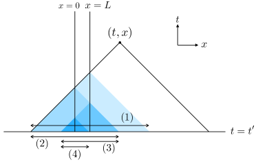
Figure 3: Domain of dependence of the Green’s function at $(t,x)$. The intervals along the horizontal axis correspond to the following step functions (i.e. the intersection of the shaded regions with the time$=t^{\prime}$ surface indicates the range of $x^{\prime}$ that gives a non-zero contribution, for $t,x$ fixed as shown):
          (1)  $\theta(t-t^{\prime}-|x-L|-|x^{\prime}-L|)$,
          (2)  $\theta(t-t^{\prime}-|x|-|x^{\prime}|),\;\theta(t-t^{\prime}-L-|x-L|-|x^{\prime}|)$,
          (3)  $\theta(t-t^{\prime}-2L-|x-L|-|x^{\prime}-L|),\;\theta(t-t^{\prime}-L-|x|-|x^{\prime}-L|)$,
          (4)  $\theta(t-t^{\prime}-2L-|x|-|x^{\prime}|),\;\theta(t-t^{\prime}-3L-|x-L|-|x^{\prime}|)$
These step functions have the interpretation of sequential scattering off
          (1)  just $V_{2}$,
          (2)  just $V_{1}$,   $V_{1}$ $\rightarrow$ $V_{2}$,
          (3)  $V_{2}$ $\rightarrow$ $V_{1}$ $\rightarrow$ $V_{2}$,   $V_{2}$ $\rightarrow$ $V_{1}$,
          (4)  $V_{1}$ $\rightarrow$ $V_{2}$ $\rightarrow$ $V_{1}$,   $V_{1}$ $\rightarrow$ $V_{2}$ $\rightarrow$ $V_{1}$ $\rightarrow$ $V_{2}$

This Green’s function may look unwieldy but can be interpreted as follows. First note that the expression in $\{\cdots\}$ encodes the quasinormal frequencies of the individual potentials. This is easiest to see in Laplace space, where for example each term in (4.16) only has (higher-order) poles at the individual quasinormal frequencies $-{V_{1}}/{2},\;-{V_{2}}/{2}$. The $k^{th}$ term in the sum comes from $k$ back-and-forth bounces between the potentials, as can be seen from the factors $e^{-s2kL}$ in Laplace space which produce a time delay $2kL$ in real space. These time delays appear in the step functions which encode the causality properties of the echo expansion. This is illustrated in Fig. 3 which shows the domain of dependence of the field at a particular point $(t,x)$ and indicates how initial data in various regions at time $t^{\prime}$ can propagate by multiple scattering to influence the field at $(t,x)$. Note that there are regions of $(t,x)$ where, by causality, only one of the potentials can contribute to the Green’s function. In these regions the field evolves in time as though there was only a single potential, even though the quasinormal spectrum of the combined system is very different from that of a single $\delta$-function. This is illustrated in Fig. 4, where we show (a) the full waveform, (b) the same Cauchy data but evolved with the Green’s function for a single potential.

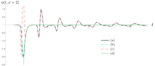
Figure 4: (a) the waveform of the solution in Figure 2 at $x=2$. (b) a solution obtained using the same Cauchy data but the Green’s function of $V_{2}$ only; note that the resulting waveform gets the first bump right but vanishes thereafter. (c) a fitting of the full waveform using the first 30 quasinormal modes (the modes with smallest $|{\rm Re}\,s|$) of the combined system. (d) the quasinormal mode of $V_{2}$ alone, fitted to the first reflected wave.

The last feature we want to mention in this section is the meaning of the quasinormal frequencies of the combined system. A collection of $\delta$-function potentials provides a particularly simple example since the Green’s function only has poles (not branch cuts) in Laplace space. This means that at sufficiently late times – once causal curves from the Cauchy data can see the entire potential – the field may be expanded as a linear combination of quasinormal modes. This can be seen in Fig. 4, where (c) shows a fit of the full waveform to a linear combination of the first 30 quasinormal modes of the combined system (the 30 modes with smallest $|{\rm Re}s|$). At late times the lowest QNF dominates. But at intermediate times multiple QNFs contribute, in a way that depends on the initial conditions for the field.

But even at late times the quasinormal frequencies of the individual potentials play a role. As discussed above each term in the echo expansion only has (higher-order) poles at the quasinormal frequencies of the individual potentials. Each echo therefore decays according to a linear combination of the quasinormal frequencies of the individual potentials, as can be seen explicitly in the coefficients of the step functions in (4.21). As a somewhat trivial example, this is illustrated for the first reflected wave in Fig. 4, where (d) shows a fit to the quasinormal mode of $V_{2}$ alone.

5 Echoes and causality

In the last section we saw that in the case of a two-delta-function potential, each echo contribution (labeled by $k$) to the Green’s function comes with a corresponding step function. The step function enforces causality, in the sense that in order for the step function to not vanish, $t-t^{\prime}$ (the separation between the time of interest $t$ and the initial time $t^{\prime}$) must be smaller than the expanded spatial distance between the point of interest $x$ and the “source” $x^{\prime}$—expanded by the extra distance traversed by $k$ echoes. We wish show in this section that essentially the same statements apply to more general disjoint potentials. As a bonus, we will see how the individual potentials govern time evolution over sufficiently short time scales.

We consider potentials of the form $V(x)=V_{1}(x)+V_{2}(x)$ where $V_{1}$ and $V_{2}$ have disjoint bounded support. We take ${\rm supp}\,V_{1}=(x_{1},x_{2})$ and ${\rm supp}\,V_{2}=(x_{3},x_{4})$ as shown below.

The separation between potentials is given by $x_{3}-x_{2}$, so the parameter $L$ has no role to play and will be dropped from all formulas in this section. Instead of an expansion in powers of $e^{-2sL}$ we perform an expansion in powers of the small quantity

$${m_{1}^{-+}m_{2}^{+-}\over m_{1}^{++}m_{2}^{++}}\,\sim\,e^{-2s(x_{3}-x_{2})}\qquad\hbox{\rm at large ${\rm Re}\,s$}$$ (5.1)

(see equation (5.5) below).

The Wronskian for the combined system $V_{1}+V_{2}$ is given by (3.31) and (3.32),

$$W_{1+2} = 2s\left(m_{2}^{++}m_{1}^{++}+m_{2}^{+-}m_{1}^{-+}\right)$$

$$= {1\over 2s}W_{1}W_{2}+2sm_{2}^{+-}m_{1}^{-+}$$

So we know how the Wronskian for the individual potentials is related to the Wronskian for the sum. From (3.33) the Green’s function for the combined system is

$$G(t,x|t^{\prime},x^{\prime})=\int_{c-i\infty}^{c+i\infty}{ds\over 2\pi i}e^{s(t-t^{\prime})}{1\over W_{1+2}}\left(\phi_{-}(s,x)\phi_{+}(s,x^{\prime})\theta(x-x^{\prime})+\phi_{+}(s,x)\phi_{-}(s,x^{\prime})\theta(x^{\prime}-x)\right)$$ (5.3)

We claim that:

All these properties can be seen in the explicit Green’s function for the case with two delta-function potentials (4.21). Let us continue the analysis for general potentials with disjoint bounded support to verify these properties. The basic fact we’ll need is that at large positive ${\rm Re}\,s$ the matching coefficients have the behavior

$${m_{1}^{-+}\over m_{1}^{++}}\,\sim\,e^{2sx_{2}}\hskip 56.9055pt{m_{2}^{+-}\over m_{2}^{++}}\,\sim\,e^{-2sx_{3}}$$ (5.5)

where we are only retaining the leading exponential dependence on $s$. We establish this behavior by a WKB analysis in appendix C. We now verify each claim in turn.

1. With the expansion (5.4), the $k=0$ term in the Green’s function (5.3) is only non-zero when $t-t^{\prime}\geq f(x,x^{\prime})$ for some $f(x,x^{\prime})$ when the contour starts to close to the left. Terms with higher $k$ come with a factor

   $$\left(\frac{m_{2}^{+-}m_{1}^{-+}}{m_{2}^{++}m_{1}^{++}}\right)^{k}\overset{s\to\infty}{\sim}e^{-2ks(x_{3}-x_{2})},$$ (5.6)

   So the $k^{th}$ term vanishes (the contour can be closed to the right) for $t-t^{\prime}<f(x,x^{\prime})+2k(x_{3}-x_{2})$. Since $2k(x_{3}-x_{2})$ is exactly the minimal time for waves to make $k$ round trips between the two potentials, we can interpret $k$ as the number of back-and-forth bounces. Moreover causality is preserved and the sum is truncated at the maximum number of bounces permitted by causality.

2. Claim II is an easy corollary. For sufficiently short times ($t-t^{\prime}<f(x,x^{\prime})+2(x_{3}-x_{2})$) only the $k=0$ term in the Green’s function contributes, so we can replace

   $${1\over W_{1+2}}\quad{\rm with}\quad{2s\over W_{1}W_{2}}$$ (5.7)

   After making this replacement poles only arise from the zeroes of $W_{1}$ and $W_{2}$, i.e. the quasinormal frequencies of the individual potentials.

3. To verify claim III we employ the uniqueness theorem. Suppose we provide Cauchy data $\phi(t^{\prime},x^{\prime})$, $\partial_{t^{\prime}}\phi(t^{\prime},x^{\prime})$ on a time slice $t^{\prime}$. Consider a point $(x,t)$ with $t>t^{\prime}$ satisfying $t-t^{\prime}<x_{3}-x$. Then the past lightcone of $(x,t)$ doesn’t make contact with $V_{2}(x)$ to the future of the Cauchy surface. This is illustrated in Fig. 5. One can use the retarded Green’s function for $V_{1}$ to construct a field by

   $$\phi(t,x)=\int dx^{\prime}\left(G_{V_{1}}(t,x|t^{\prime},x^{\prime})\partial_{t^{\prime}}\phi(t^{\prime},x^{\prime})-\partial_{t}G_{V_{1}}(t,x|t^{\prime},x^{\prime})\phi(t^{\prime},x^{\prime})\right).$$ (5.8)

   It is obvious that this solves the equation of motion for $t-t^{\prime}<x_{3}-x$ and also satisfies the initial conditions at $t^{\prime}$. Due to the uniqueness theorem this solution is unique therefore the retarded Green’s function $G_{V_{1}}$ we used must equal the full retarded Green’s function $G_{V_{1}+V_{2}}$ within this spacetime domain. Mismatch between $G_{V_{1}}$ and $G_{V_{1}+V_{2}}$ occurs when $t-t^{\prime}>x_{3}-x$ since $G_{V_{1}}$ does not solve the Green’s function equation of motion in the red region depicted in Fig. 5.

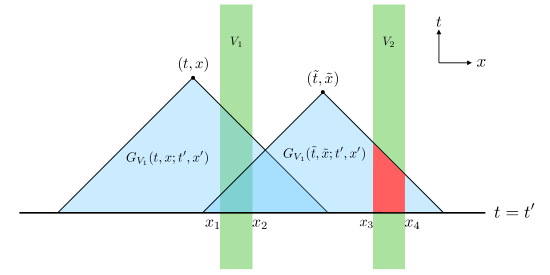
Figure 5: Cauchy data is given on the time slice $t^{\prime}$. The retarded Green’s function for $V_{1}$, $G_{V_{1}}$, has support in the past lightcone of the indicated points. The red area is where $G_{V_{1}}$ fails to solve $(\partial_{t}^{2}-\partial_{x}^{2}+V_{2}(x))G_{V_{1}}=\delta(t-t^{\prime})\delta(x-x^{\prime})$.

6 Discussion and conclusion

In this work we have explored simple potential models to develop a better understanding of quasinormal modes. There are several lessons we can draw from our analysis.

First, the basic object of interest is the retarded Green’s function. In real space the retarded Green’s function vanishes for $t<t^{\prime}$, which in Laplace space requires that we impose the boundary conditions (3.10), (3.11). In this approach to constructing the Green’s function, the quasinormal frequencies arise as derived quantities: they are simply the poles of the Green’s function in Laplace space. These poles are associated with modes that obey outgoing (or radiative) boundary conditions, since as pointed out below (3.25) they correspond to homogeneous solutions with the behavior $\sim e^{s(t-|x|)}$ as $x\rightarrow\pm\infty$. So quasinormal boundary conditions arise naturally, as a consequence of constructing a retarded Green’s function. The fact that quasinormal boundary conditions arise in this way fits with the intuition that – barring bound states – any localized excitation should end up as outgoing radiation.

In this way we are led to construct quasinormal modes with the peculiar feature that they grow exponentially at spatial infinity. This follows from the fact that in a stable system the quasinormal frequencies must have ${\rm Re}\,s<0$ so that fields decay with time. As a result quasinormal modes grow exponentially at spatial infinity, as follows in general from (3.10), (3.11) and can be seen in the example of a $\delta$-function potential in (2.2). Does it make sense to expand a Green’s function in terms of modes that grow at spatial infinity?

To see that this isn’t a problem, note that causality prevents the exponential growth from showing up in the retarded Green’s function. The retarded Green’s function $G(t,x|t^{\prime},x^{\prime})$ is only non-zero in the future light-cone of $(t^{\prime},x^{\prime})$, which eliminates the problematic regime $|x|\rightarrow\infty$. For a single $\delta$-function this can be seen in the last line of (4.9), which indeed grows exponentially with $|x|$ but gets cut off by causality when $|x|$ reaches the relevant light cone. This can also be seen in (4.21), where the step functions cut off the exponential growth with $|x|$ and in fact require that all of the exponents appearing in (4.21) are negative.

Causality plays another important role: over a finite time interval, it limits the way in which the potential can contribute to time evolution. For example, as pointed out in section 5, for two disjoint potentials the sum over echoes is truncated to the maximum number permitted by causality. A related point is that if the other potential is distant enough to be out of causal contact then it can be ignored. This is true even though the quasinormal frequencies of the combined system (which are globally-defined quantities that don’t know about causality) are very sensitive to distant perturbations. This is relevant to the recent computations of the quasinormal spectrum of exotic compact objects [12, 13, 14, 15, 16, 17, 18, 19], where the spectrum differs greatly from that of the corresponding black hole, yet the initial waveform (generated by an infalling test particle for example) can be very similar (e.g. [12]). The lesson is that over finite times it is not enough to consider the spectrum of quasinormal frequencies (of the combined system) by themselves. One also has to take causality into account. This can be done by making an echo expansion of the form (5.4), in which poles only arise at the quasinormal frequencies of the individual potentials.

In this paper we considered potentials with disjoint bounded support to make the analysis tractable. But causality should be respected in general, with observational as well as theoretical implications. On the observational side it means that in any practical measurement of the gravitational waves from a merger, the ringdown will be governed by the quasinormal frequencies of the resulting black hole and not by distant perturbations to the potential such as from the surrounding stars (assuming the ringdown can only be observed for a finite small time interval after merger). As a theoretical example, for black holes in anti-de Sitter space the Regge-Wheeler potential grows far from the black hole, and this changes the quasinormal spectrum compared to flat space [35]. But over short times and distances (much less than an AdS radius) a small black hole in AdS is not sensitive to the asymptotic potential and to a good approximation perturbations will be governed by the same quasinormal spectrum as in Minkowski space.

We’ve seen that over a finite time interval distant perturbations to the potential (meaning perturbations that are out of causal contact) have no effect. This leaves the question of the effect of local perturbations to the potential (meaning perturbations that are permitted to contribute by causality). Can we characterize whether local perturbations to the potential have a large or small effect? This has applications, for example, to observational signatures of modifications to the near-horizon region of black holes (e.g. [36, 37, 38]). Although not the main focus of our work, there are some conclusions we can draw. Consider for example the pair of $\delta$-functions (2.3). Regarding $V_{2}$ as a perturbation, and assuming the separation $L$ is small so that $V_{2}$ is permitted to contribute by causality, is there a sense in which a small value of $V_{2}$ has a small effect? Note that the quasinormal frequencies of the combined system are not a good guide since they change dramatically as soon as $V_{2}\not=0$. Instead we return to the causal expansion (4.21). Gathering terms with like powers of $V_{2}$ we see that there are actually two dimensionless expansion parameters. One dimensionless combination, arising from the exponentials in the numerators, is

$$V_{2}\big{(}t-t_{\rm lc}\big{)}$$ (6.1)

Here $t_{\rm lc}$ is the time at which the relevant light cone first reaches the point $x$. Another dimensionless combination, arising from the denominators in (4.21), is $V_{2}/V_{1}$. So for $V_{2}$ to have a small effect we require both

$${V_{2}\over V_{1}}\ll 1\qquad V_{2}\big{(}t-t_{\rm lc}\big{)}\ll 1$$ (6.2)

The first condition is not surprising; it just says that $V_{1}$ is the dominant potential. Assuming that’s the case, to interpret the second condition, what value should we take for $t-t_{\rm lc}$? Since $V_{1}$ dominates, the signal which is initially detected decays on a timescale set by the quasinormal frequencies of $V_{1}$. For a realistic system (not a $\delta$-function potential) these frequencies are set by the light-crossing time for the system. So in deciding whether the perturbation $V_{2}$ can appreciably affect the initial signal, the relevant control parameter (besides $V_{2}\ll V_{1}$) is

$$V_{2}\times\hbox{\rm(light-crossing time)}$$ (6.3)

If this parameter is small then the initial signal is not appreciably distorted by the perturbation. Of course even if this parameter is small the perturbation produces late-time echoes that could in principle be detected.

Acknowledgements

We thank Emanuele Berti, Vitor Cardoso, Austin Joyce, Alberto Nicolis, Paolo Pani, Rachel Rosen, Luca Santoni and Michael Zlotnikov for discussions. LH acknowledges support from NASA NXX16AB27G and DOE DE-SC011941. DK thanks the Columbia University Center for Theoretical Physics for hospitality during this work. The work of DK is supported by U.S. National Science Foundation grant PHY-1820734. SW is supported in part by the Croucher Foundation.

Appendix A Green’s function solution to the wave equation

In this appendix we collect some properties of Green’s functions as applied to wave equations.

We first recall how a Green’s function can be used to evolve Cauchy data. Note that if $[\partial_{t}^{2}-\partial_{x}^{2}+V(x)]G(t,x|t^{\prime},x^{\prime})=\delta(t-t^{\prime})\delta(x-x^{\prime})$, then $[\partial_{t^{\prime}}^{2}-\partial_{x^{\prime}}^{2}+V(x^{\prime})]G(t,x^{\prime}|t^{\prime},x)=\delta(t-t^{\prime})\delta(x-x^{\prime})$. (Note also $G$ is a function of $t-t^{\prime},x,x^{\prime}$ alone.) Applying the second equation to the quantity

$$\int_{t_{0}}^{\infty}\int_{-\infty}^{\infty}dx^{\prime}\phi(t^{\prime},x^{\prime})[\partial_{t^{\prime}}^{2}-\partial_{x^{\prime}}^{2}+V(x^{\prime})]G(t,x^{\prime}|t^{\prime},x)-G(t,x^{\prime}|t^{\prime},x)[\partial_{t^{\prime}}^{2}-\partial_{x^{\prime}}^{2}+V(x^{\prime})]\phi(t^{\prime},x^{\prime})\,,$$

with $t_{0}<t$, one can see that this quantity is $\phi(t,x)$. On the other hand, integrating by parts, and assuming $G$ and $\phi$ vanishes as $x^{\prime}\rightarrow\pm\infty$, and $G$ and $\partial_{t^{\prime}}G$ vanishes as $t^{\prime}\rightarrow\infty$, one sees that the same quantity gives

$$\int_{-\infty}^{\infty}dx^{\prime}[G(t,x^{\prime}|t_{0},x)\partial_{t_{0}}\phi(t_{0},x^{\prime})-\phi(t_{0},x^{\prime})\partial_{t_{0}}G(t,x^{\prime}|t_{0},x)]\,.$$

The Green’s function satisfies reciprocity,

$$G(t,x^{\prime}|t_{0},x)=G(t,x|t_{0},x^{\prime})$$ (A.1)

which lets us switch $x$ and $x^{\prime}$. Making this switch, and relabeling $t_{0}$ as $t^{\prime}$, yields Eq. (3.26).

Next we check that Fourier analysis gives rise to an equivalent formula for evolving Cauchy data. For simplicity we specialize to the free wave equation

$$(\partial_{t}^{2}-\partial_{x}^{2})\phi(t,x)=0$$ (A.2)

It is easy to see that a given Fourier mode must have either cosine or sine dependence on time $t$, and thus the evolution from $t^{\prime}$ to $t$ is given by:

$$\phi(t,x)=\int{dk\over 2\pi}e^{-ikx}\left(\phi(t^{\prime},k){\,\rm cos\,}(k[t-t^{\prime}])+\partial_{t^{\prime}}\phi(t^{\prime},k)\,{{\,\rm sin\,}(k[t-t^{\prime}])\over k}\right)\,,$$ (A.3)

where $\phi(t^{\prime},k)=\int dx^{\prime}\phi(t^{\prime},x^{\prime})e^{ik^{\prime}x^{\prime}}$. To see that this is consistent with the general evolution formula Eq. (3.26), with the free retarded Green’s function $(1/2)\theta(t-t^{\prime}-|x-x^{\prime}|)$, it is useful to note that

$$\int{dk\over 2\pi}\theta(t-t^{\prime}){{\,\rm sin\,}(k[t-t^{\prime}])\over k}e^{ik(x-x^{\prime})}={1\over 2}\theta(t-t^{\prime}-|x-x^{\prime}|)\,,$$ (A.4)

which can be derived by rewriting $k^{-1}{\,\rm sin\,}(k[t-t^{\prime}])=\int_{-(t-t^{\prime})}^{t-t^{\prime}}dy\,e^{iky}/2$. This is also consistent with the fact that $\theta(t-t^{\prime}){{\,\rm sin\,}(k[t-t^{\prime}])\over k}$ solves $(\partial_{t}^{2}+k^{2})G(t-t^{\prime},k)=\delta(t-t^{\prime})$.

Appendix B An alternate method for a multiple $\delta$-function potential

In this appendix we provide the exact solution for the Green’s function of (3.1) with a multiple $\delta$-function potential,

$$\left(\partial_{t}^{2}-\partial_{x}^{2}+\sum_{i}V_{i}\delta(x-x_{i})\right)G(t,x|t^{\prime},x^{\prime})=\delta(t-t^{\prime})\delta(x-x^{\prime}),$$ (B.1)

$$\qquad G(t,x|t^{\prime},x^{\prime})=\partial_{t}G(t,x|t^{\prime},x^{\prime})=0\quad\mbox{for}\quad t<t^{\prime}$$ (B.2)

With a Laplace transform in $t-t^{\prime}$ and Fourier transform in $x$, $\tilde{G}_{s,k}(x^{\prime})=\int_{0^{-}}^{\infty}dt\int_{-\infty}^{\infty}dxe^{-st+ikx}G(t,x|0,x^{\prime})$,

$$(s^{2}+k^{2})\tilde{G}_{s,k}(x^{\prime})+\sum_{i}V_{i}e^{ikx_{i}}G(s;x_{i}|x^{\prime})=e^{ikx^{\prime}}.$$ (B.3)

After inverse Fourier transform and solving for $G(s;x|x^{\prime})$ we obtain

$$G(s;x|x^{\prime})=\frac{e^{-s|x-x^{\prime}|}}{2s}-\sum_{i}V_{i}G(s;x_{i}|x^{\prime})\frac{e^{-s|x-x_{i}|}}{2s},$$ (B.4)

where $G(s;x_{i}|x^{\prime})$ is solved as

$$G(s;x_{i}|x^{\prime})=\sum_{j}(M^{-1})_{ij}\frac{e^{-s|x_{j}-x^{\prime}|}}{2s},$$

$$M_{ij}=\left\{\begin{array}[]{ll}1+\frac{V_{i}}{2s}&i=j\\ V_{j}\frac{e^{-s|x_{j}-x_{i}|}}{2s}&i\neq j\end{array}\right..$$ (B.7)

With a potential composed of two delta functions, $V(x)=V_{1}\delta(x)+V_{2}\delta(x-L)$, one can easily obtain

$$G(s;x|x^{\prime}) =\frac{1}{2s}e^{-s|x-x^{\prime}|}$$

$$\quad+\frac{V_{1}(2s+V_{2})e^{-s(|x|+|x^{\prime}|)}-V_{1}V_{2}e^{-s(|x|+|L|+|L-x^{\prime}|)}}{2s\left[V_{1}V_{2}e^{-2s|L|}-(2s+V_{1})(2s+V_{2})\right]}$$

$$\quad+\frac{V_{2}(2s+V_{1})e^{-s(|L-x|+|L-x^{\prime}|)}-V_{1}V_{2}e^{-s(|L-x|+|L|+|x^{\prime}|)}}{2s\left[V_{1}V_{2}e^{-2s|L|}-(2s+V_{1})(2s+V_{2})\right]},$$ (B.8)

This reproduces (4) without having to solve for $\phi_{+}$, $\phi_{-}$.

Appendix C WKB approximation for the matching coefficients

In this appendix we use the WKB approximation to obtain an estimate for the matching coefficients (3.22) at large positive ${\rm Re}\,s$ and show that their ratios satisfy (5.5).

For a potential with compact support, ${\rm supp}\,V=(x_{1},x_{2})$, we want to solve

$$\left(-\partial_{x}^{2}+s^{2}+V(x)\right)\phi(x)=0$$ (C.1)

If $s$ is large the effective potential $s^{2}+V(x)$ varies adiabatically with $x$. Then the WKB approximation should be valid, and we can write down a WKB solution with the behavior (3.10) needed for $\phi_{+}$.

$$\phi(x)=\left\{\begin{array}[]{ll}e^{sx}&\quad x<x_{1}\\ a\,e^{\int_{x_{1}}^{x}dx^{\prime}\,\sqrt{s^{2}+V(x^{\prime})}}+b\,e^{-\int_{x_{1}}^{x}dx^{\prime}\,\sqrt{s^{2}+V(x^{\prime})}}&\quad x_{1}<x<x_{2}\\ m^{++}e^{sx}+m^{-+}e^{-sx}&\quad x>x_{2}\end{array}\right.$$ (C.2)

Requiring that $\phi(x)$ and $\partial_{x}\phi(x)$ be continuous at $x_{1}$ and $x_{2}$ fixes the coefficients, in particular

$$m^{++} = {1\over 4}e^{-s(x_{2}-x_{1})}e^{\int_{x_{1}}^{x_{2}}dx^{\prime}\,\sqrt{s^{2}+V(x^{\prime})}}\left(1+{s\over\sqrt{s^{2}+V(x_{1})}}\right)\left(1+{\sqrt{s^{2}+V(x_{2})}\over s}\right)$$ (C.3)

$$\!\!\!\!\!+\,{1\over 4}e^{-s(x_{2}-x_{1})}e^{-\int_{x_{1}}^{x_{2}}dx^{\prime}\,\sqrt{s^{2}+V(x^{\prime})}}\left(1-{s\over\sqrt{s^{2}+V(x_{1})}}\right)\left(1-{\sqrt{s^{2}+V(x_{2})}\over s}\right)$$

$$m^{-+} = {1\over 4}e^{s(x_{1}+x_{2})}e^{\int_{x_{1}}^{x_{2}}dx^{\prime}\,\sqrt{s^{2}+V(x^{\prime})}}\left(1+{s\over\sqrt{s^{2}+V(x_{1})}}\right)\left(1-{\sqrt{s^{2}+V(x_{2})}\over s}\right)$$ (C.4)

$$\!\!\!\!\!+\,{1\over 4}e^{s(x_{1}+x_{2})}e^{-\int_{x_{1}}^{x_{2}}dx^{\prime}\,\sqrt{s^{2}+V(x^{\prime})}}\left(1-{s\over\sqrt{s^{2}+V(x_{1})}}\right)\left(1+{\sqrt{s^{2}+V(x_{2})}\over s}\right)$$

As ${\rm Re}\,s\rightarrow+\infty$ this means

$$m^{++}\,\sim\,1\hskip 56.9055ptm^{-+}\,\sim\,e^{2sx_{2}}$$ (C.5)

where we are keeping track of the leading exponential dependence on $s$. A similar calculation for $\phi_{-}$ gives

$$m^{+-} = {1\over 4}e^{-s(x_{1}+x_{2})}e^{\int_{x_{1}}^{x_{2}}dx^{\prime}\,\sqrt{s^{2}+V(x^{\prime})}}\left(1-{s\over\sqrt{s^{2}+V(x_{1})}}\right)\left(1+{\sqrt{s^{2}+V(x_{2})}\over s}\right)$$ (C.6)

$$\!\!\!\!\!+\,{1\over 4}e^{-s(x_{1}+x_{2})}e^{-\int_{x_{1}}^{x_{2}}dx^{\prime}\,\sqrt{s^{2}+V(x^{\prime})}}\left(1+{s\over\sqrt{s^{2}+V(x_{1})}}\right)\left(1-{\sqrt{s^{2}+V(x_{2})}\over s}\right)$$

and implies

$$m^{+-}\,\sim\,e^{-2sx_{1}}$$ (C.7)

Given these results, which can be applied to $V_{1}$ and $V_{2}$ separately, the ratios (5.5) follow.

References

- [1] LIGO Scientific, Virgo , B. P. Abbott et al., “Binary Black Hole Mergers in the first Advanced LIGO Observing Run,” Phys. Rev. X6 (2016) no. 4, 041015, arXiv:1606.04856 [gr-qc]. [erratum: Phys. Rev.X8,no.3,039903(2018)].
- [2] K. D. Kokkotas and B. G. Schmidt, “Quasinormal modes of stars and black holes,” Living Rev. Rel. 2 (1999) 2, arXiv:gr-qc/9909058 [gr-qc].
- [3] E. Berti, V. Cardoso, and A. O. Starinets, “Quasinormal modes of black holes and black branes,” Class. Quant. Grav. 26 (2009) 163001, arXiv:0905.2975 [gr-qc].
- [4] T. Regge and J. A. Wheeler, “Stability of a Schwarzschild singularity,” Phys. Rev. 108 (1957) 1063–1069.
- [5] F. J. Zerilli, “Effective potential for even parity Regge-Wheeler gravitational perturbation equations,” Phys. Rev. Lett. 24 (1970) 737–738.
- [6] S. A. Teukolsky, “Perturbations of a rotating black hole. 1. Fundamental equations for gravitational electromagnetic and neutrino field perturbations,” Astrophys. J. 185 (1973) 635–647.
- [7] E. Berti and V. Cardoso, “Quasinormal ringing of Kerr black holes. I. The Excitation factors,” Phys. Rev. D74 (2006) 104020, arXiv:gr-qc/0605118 [gr-qc].
- [8] Z. Zhang, E. Berti, and V. Cardoso, “Quasinormal ringing of Kerr black holes. II. Excitation by particles falling radially with arbitrary energy,” Phys. Rev. D88 (2013) 044018, arXiv:1305.4306 [gr-qc].
- [9] H.-P. Nollert, “About the significance of quasinormal modes of black holes,” Phys. Rev. D53 (1996) 4397–4402, arXiv:gr-qc/9602032 [gr-qc].
- [10] H.-P. Nollert and R. H. Price, “Quantifying excitations of quasinormal mode systems,” J. Math. Phys. 40 (1999) 980–1010, arXiv:gr-qc/9810074 [gr-qc].
- [11] E. Barausse, V. Cardoso, and P. Pani, “Can environmental effects spoil precision gravitational-wave astrophysics?,” Phys. Rev. D89 (2014) no. 10, 104059, arXiv:1404.7149 [gr-qc].
- [12] V. Cardoso, E. Franzin, and P. Pani, “Is the gravitational-wave ringdown a probe of the event horizon?,” Phys. Rev. Lett. 116 (2016) no. 17, 171101, arXiv:1602.07309 [gr-qc]. [Erratum: Phys. Rev. Lett.117,no.8,089902(2016)].
- [13] V. Cardoso, S. Hopper, C. F. B. Macedo, C. Palenzuela, and P. Pani, “Gravitational-wave signatures of exotic compact objects and of quantum corrections at the horizon scale,” Phys. Rev. D94 (2016) no. 8, 084031, arXiv:1608.08637 [gr-qc].
- [14] J. T. G. Ghersi, A. V. Frolov, and D. A. Dobre, “Echoes from the scattering of wavepackets on wormholes,” arXiv:1901.06625 [gr-qc].
- [15] V. Cardoso and P. Pani, “The observational evidence for horizons: from echoes to precision gravitational-wave physics,” arXiv:1707.03021 [gr-qc].
- [16] Q. Wang, N. Oshita, and N. Afshordi, “Echoes from Quantum Black Holes,” arXiv:1905.00446 [gr-qc].
- [17] R. H. Price and G. Khanna, “Gravitational wave sources: reflections and echoes,” Class. Quant. Grav. 34 (2017) no. 22, 225005, arXiv:1702.04833 [gr-qc].
- [18] Z. Mark, A. Zimmerman, S. M. Du, and Y. Chen, “A recipe for echoes from exotic compact objects,” Phys. Rev. D96 (2017) no. 8, 084002, arXiv:1706.06155 [gr-qc].
- [19] P. Bueno, P. A. Cano, F. Goelen, T. Hertog, and B. Vercnocke, “Echoes of Kerr-like wormholes,” Phys. Rev. D97 (2018) no. 2, 024040, arXiv:1711.00391 [gr-qc].
- [20] E. W. Leaver, “Spectral decomposition of the perturbation response of the Schwarzschild geometry,” Phys. Rev. D34 (1986) 384–408.
- [21] H.-P. Nollert and B. G. Schmidt, “Quasinormal modes of Schwarzschild black holes: Defined and calculated via Laplace transformation,” Phys. Rev. D45 (1992) no. 8, 2617.
- [22] N. Andersson, “Excitation of Schwarzschild black hole quasinormal modes,” Phys. Rev. D51 (1995) 353–363.
- [23] N. Szpak, “Quasinormal mode expansion and the exact solution of the Cauchy problem for wave equations,” arXiv:gr-qc/0411050 [gr-qc].
- [24] M. R. Correia and V. Cardoso, “Characterization of echoes: A Dyson-series representation of individual pulses,” Phys. Rev. D97 (2018) no. 8, 084030, arXiv:1802.07735 [gr-qc].
- [25] Y.-X. Huang, J.-C. Xu, and S.-Y. Zhou, “The Fredholm Approach to Charactize Gravitational Wave Echoes,” arXiv:1908.00189 [gr-qc].
- [26] V. Cardoso, V. F. Foit, and M. Kleban, “Gravitational wave echoes from black hole area quantization,” arXiv:1902.10164 [hep-th].
- [27] Z.-P. Li and Y.-S. Piao, “Mixing of gravitational wave echoes,” arXiv:1904.05652 [gr-qc].
- [28] L. Buoninfante, A. Mazumdar, and J. Peng, “Nonlocality amplifies echoes,” arXiv:1906.03624 [gr-qc].
- [29] M. Mirbabayi, “The Quasinormal Modes of Quasinormal Modes,” arXiv:1807.04843 [gr-qc].
- [30] E. S. C. Ching, P. T. Leung, W. M. Suen, and K. Young, “Late time tail of wave propagation on curved space-time,” Phys. Rev. Lett. 74 (1995) 2414–2417, arXiv:gr-qc/9410044 [gr-qc].
- [31] E. S. C. Ching, P. T. Leung, W. M. Suen, and K. Young, “Wave propagation in gravitational systems: Late time behavior,” Phys. Rev. D52 (1995) 2118–2132, arXiv:gr-qc/9507035 [gr-qc].
- [32] D. Skinner, “Green’s Functions for ODEs,”. http://www.damtp.cam.ac.uk/user/dbs26/1Bmethods.html.
- [33] E. S. C. Ching, P. T. Leung, W. M. Suen, and K. Young, ‘‘Wave propagation in gravitational systems: Completeness of quasinormal modes,’’ Phys. Rev. D54 (1996) 3778--3791, arXiv:gr-qc/9507034 [gr-qc].
- [34] E. S. C. Ching, P. T. Leung, A. Maassen van den Brink, W. M. Suen, S. S. Tong, and K. Young, ‘‘Quasinormal-mode expansion for waves in open systems,’’ Rev. Mod. Phys. 70 (1998) 1545, arXiv:gr-qc/9904017 [gr-qc].
- [35] G. T. Horowitz and V. E. Hubeny, ‘‘Quasinormal modes of AdS black holes and the approach to thermal equilibrium,’’ Phys. Rev. D62 (2000) 024027, arXiv:hep-th/9909056 [hep-th].
- [36] O. J. Tattersall, P. G. Ferreira, and M. Lagos, ‘‘General theories of linear gravitational perturbations to a Schwarzschild Black Hole,’’ Phys. Rev. D97 (2018) no. 4, 044021, arXiv:1711.01992 [gr-qc].
- [37] G. Franciolini, L. Hui, R. Penco, L. Santoni, and E. Trincherini, ‘‘Effective Field Theory of Black Hole Quasinormal Modes in Scalar-Tensor Theories,’’ JHEP 02 (2019) 127, arXiv:1810.07706 [hep-th].
- [38] R. McManus, E. Berti, C. F. B. Macedo, M. Kimura, A. Maselli, and V. Cardoso, ‘‘Parametrized black hole quasinormal ringdown. II. Coupled equations and quadratic corrections for nonrotating black holes,’’ Phys. Rev. D100 (2019) no. 4, 044061, arXiv:1906.05155 [gr-qc].