Algebraic structure of the range of a trigonometric polynomial

Abstract.

The range of a trigonometric polynomial with complex coefficients can be interpreted as the image of the unit circle under a Laurent polynomial. We show that this range is contained in a real algebraic subset of the complex plane. Although the containment may be proper, the difference between the two sets is finite, except for polynomials with certain symmetry.

1. Introduction

In 1976 Quine [6, Theorem 1] proved that the image of the unit circle $\mathbb{T}$ under an algebraic polynomial $p$ of degree $n$ is contained in a real algebraic set $V=\{(x,y)\in\mathbb{R}^{2}\colon q(x,y)=0\}$ where $q$ is a polynomial of degree $2n$. In general $p(\mathbb{T})$ is a proper subset of $V$, but we will show that $V\setminus p(\mathbb{T})$ is finite, and that $V=p(\mathbb{T})$ whenever $V$ is connected.

Consider a trigonometric polynomial $P(t)=\sum_{k=-m}^{n}a_{k}e^{ikt}$, $t\in\mathbb{R}$, with complex coefficients $a_{k}$. It is natural to require $a_{-m}a_{n}\neq 0$ here. The range of $P$ is precisely the image of the unit circle $\mathbb{T}$ under the Laurent polynomial $p(z)=\sum_{k=-m}^{n}a_{k}z^{k}$. This motivates our investigation of $p(\mathbb{T})$ for Laurent polynomials. Our main result, Theorem 2.1, asserts that $p(\mathbb{T})$ is contained in the zero set $V$ of a polynomial of degree $2\max(m,n)$. This matches Quine’s theorem in the case of $p$ being an algebraic polynomial, i.e., $m=0$. The difference $V\setminus p(\mathbb{T})$ is finite when $m\neq n$, but may be infinite when $m=n$.

In Section 4 we investigate the exceptional case when $V\setminus p(\mathbb{T})$ is infinite, and relate it to the properties of the zero set of a certain harmonic rational function. The structure of zero sets of such functions is a topic of current interest with applications to gravitational lensing [1, 2].

Finally, in Section 5 we use the algebraic nature of the polynomial images of $\mathbb{T}$ to estimate the number of intersections of two such images, i.e., the number of shared values of two trigonometric polynomials.

2. Algebraic nature of polynomial images of circles

By definition, a real algebraic subset of $\mathbb{R}^{2}$ is a set of the form $\{(x,y)\in\mathbb{R}^{2}\colon q(x,y)=0\}$ where $q\in\mathbb{R}[x,y]$ is a polynomial in $x,y$. Consider a Laurent polynomial

(2.1) $$p(z)=\sum_{k=-m}^{n}a_{k}z^{k},\quad z\in\mathbb{C}\setminus\{0\},$$

where $m\geq 0$, $n\geq 1$, and $a_{-m}a_{n}\neq 0$. This includes the case of algebraic polynomials ($m=0$), because the condition $a_{0}\neq 0$ can be ensured by adding a constant to $p$, which does not affect the algebraic nature of $p(\mathbb{T})$. Since we are interested in the image of the unit circle, which is invariant under the substitution of $z^{-1}$ for $z$, it suffices to consider the case $m\leq n$.

Theorem 2.1.

Let $p$ be the Laurent polynomial (2.1) with $m\leq n$.

1. The image of $\mathbb{T}$ under $p$, is contained in the zero set $V$ of some polynomial $h\in\mathbb{R}[x,y]$ of degree $2n$.

2. If $h$ is expressed as a polynomial $h_{\mathbb{C}}\in\mathbb{C}[w,\overline{w}]$ via the substitution $w=x+iy$, the degree of $h_{\mathbb{C}}$ in each of the variables $w$ and $\overline{w}$ separately is $m+n$.

3. If $m<n$, then the set $V\setminus p(\mathbb{T})$ is finite.

4. In the case $m=n$ the set $V\setminus p(\mathbb{T})$ is finite if and only if $V$ is bounded.

The proof of Theorem 2.1 involves two polynomials

(2.2) $$g(z)=z^{m}(p(z)-w)\quad\text{and}\quad g^{*}(z)=z^{n+m}\overline{g(1/\bar{z})}=z^{n}\overline{(p(1/\bar{z})-w)}$$

which are the subject of the following lemma.

Lemma 2.2.

The resultant $h_{\mathbb{C}}=\operatorname{res}(g,g^{*})$ of the polynomials (2.2) is a polynomial in $\mathbb{C}[w,\overline{w}]$ of degree $2n$. Moreover, $h_{\mathbb{C}}$ has degree $m+n$ in each of the variables $w$ and $\overline{w}$ separately. Finally, $h(x,y):=h_{\mathbb{C}}(x+iy,x-iy)$ is a polynomial of degree $2n$ in $\mathbb{R}[x,y]$.

Proof.

Both $g$ and $g^{*}$ are polynomials of degree $m+n$ in $z$, except for the case $m=0$ and $w=a_{0}$ which we ignore in this proof because considering a generic $w$ is enough. By definition, the resultant of $g$ and $g^{*}$ is the determinant of the following matrix of size $2(m+n)$.

(2.3) $$R=\begin{pmatrix}a_{-m}&\cdots&\cdots&a_{0}-w&\cdots&a_{n}&0&0\\ 0&\ddots&&&\ddots&&\ddots&0\\ 0&0&a_{-m}&\cdots&\cdots&a_{0}-w&\cdots&a_{n}\\ \overline{a_{n}}&\cdots&\overline{a_{0}}-\overline{w}&\cdots&\cdots&\overline{a_{-m}}&0&0\\ 0&\ddots&&\ddots&&&\ddots&0\\ 0&0&\overline{a_{n}}&\cdots&\overline{a_{0}}-\overline{w}&\cdots&\cdots&\overline{a_{-m}}\\ \end{pmatrix}$$

All appearances of $w$ or $\overline{w}$ in $R$ are in the columns numbered $m+1$ through $m+2n$, which are the middle $2n$ columns of matrix $R$. Therefore, $h_{\mathbb{C}}$ is a polynomial of degree at most $2n$.

Let us first prove that $h_{\mathbb{C}}$ has degree $n+m$ in each variable separately. It obviously cannot be greater than $n+m$, since each of $w$ and $\overline{w}$ appears $n+m$ times in the matrix. The position of $a_{0}-w$ in the top half of the matrix shows that the Leibniz formula for $\det R$ contains the term $\pm\overline{a_{n}}^{m}\overline{a_{-m}}^{n}(a_{0}-w)^{n+m}$ and no other terms with the monomial $w^{n+m}$. Therefore, the coefficient of $w^{n+m}$ in $h$ is $\pm\overline{a_{n}}^{m}\overline{a_{-m}}^{n}\neq 0$. Similarly, the coefficient of $\overline{w}^{2n}$ in $h$ is $\pm a_{-m}^{n}a_{n}^{m}\neq 0$. This proves that $h_{\mathbb{C}}$ has degree $n+m$ in $w$ and $\overline{w}$ separately.

When $m=n$, the preceding paragraph shows that $h_{\mathbb{C}}$ has degree $2n$ in $w$ and $\overline{w}$ separately, which implies $\deg h=2n$.

We proceed to prove $\deg h_{\mathbb{C}}=2n$ in the case $m<n$. Let $R_{1}$ be the matrix obtained from $R$ by replacing all constant entries in the columns $m+1,\dots,m+2n$ by $0$. Since the cofactor of any of the entries we replaced is a polynomial of degree less than $2n$, the difference $\det R-\det R_{1}$ has degree less than $2n$. Thus, it suffices to show that $\det R_{1}$ has degree $2n$. When deriving a formula for $\det R_{1}$ we may assume $w\neq a_{0}$. Let us focus on the columns of $R_{1}$ numbered $m+1,\dots,2m$: the only nonzero entries at these columns are:

• $a_{0}-w$ at $(j-m,j)$ for $m+1\leq j\leq 2m$;

• $\overline{a_{0}}-\overline{w}$ at $(j+m,j)$ for $n+1\leq j\leq 2m$.

We can use column operations to eliminate all nonzero entries in the upper-left $m\times m$ submatrix of $R_{1}$. Since this submatrix is upper-triangular, the process only involves adding some multiples of $j$th column with $m+1\leq j\leq 2m$ to columns numbered $k$ where $j-m\leq k\leq m$. Such a column operation also affects the bottom half of the matrix, where we add a multiple of the entry $(j+m,j)$ to the entry $(j+m,k)$. Since $(j+m)-k\leq j+m-(j-m)=2m<n+m$, the affected entries of the bottom half are strictly above the diagonal $\{(n+m+j,j)\colon 1\leq j\leq m\}$ which is filled with the value $a_{n}$. In conclusion, these column operations do not substantially affect the upper-triangular submatrix formed by the entries $(i,j)$ with $n+m+1\leq i\leq n+2m$, $1\leq j\leq m$, in the sense that the submatrix remains upper-triangular and its diagonal entries remain equal to $a_{n}$.

Similar column operations on the right side of the matrix eliminate all nonzero entries in the bottom right $m\times m$ submatrix of $R_{1}$. Let $R_{2}$ be the resulting matrix:

$$R_{2}=\begin{pmatrix}0&\cdots&a_{0}-w&\cdots&\cdots&0&0&0\\ 0&\ddots&&\ddots&&&\ddots&0\\ 0&0&0&\cdots&a_{0}-w&\cdots&\cdots&a_{n}\\ \overline{a_{n}}&\cdots&\cdots&\overline{a_{0}}-\overline{w}&\cdots&0&0&0\\ 0&\ddots&&&\ddots&&\ddots&0\\ 0&0&0&\cdots&\cdots&\overline{a_{0}}-\overline{w}&\cdots&0\\ \end{pmatrix}$$

We claim that $\det R_{2}=\pm|a_{n}|^{2m}|a_{0}-w|^{2n}$. Indeed, the first $m$ columns of $R_{2}$ contain only an upper-triangular submatrix with $\overline{a_{n}}$ on the diagonal; the last $m$ columns contain only a lower-triangular matrix with $a_{n}$ on the diagonal. After these are accounted for, we are left with a $2n\times 2n$ submatrix in which every row has exactly one nonzero element, either $a_{0}-w$ or its conjugate. This completes the proof of $\deg h_{\mathbb{C}}=2n$.

Define $h(x,y)=h_{\mathbb{C}}(x+iy,x-iy)$ for real $x,y$. We claim that $h$ is real-valued, and thus has real coefficients. Recall (e.g., [4, p. 11]) that the resultant can be expressed in terms of the roots of the polynomials $g,g^{*}$. Let $z_{1},\dots,z_{n+m}$ be the roots of $g$ listed with multiplicity. To simplify notation, we separate the cases $m>0$ and $m=0$.

Case $m>0$. We have $\prod_{k=1}^{m+n}z_{k}=(-1)^{n+m}a_{-m}/a_{n}$; in particular, $z_{k}\neq 0$ for all $k$. It follows from (2.2) that $g^{*}$ has roots $1/\overline{z_{k}}$ for $k=1,\dots,n+m$. The leading terms of $g$ and $g^{*}$ are $a_{n}$ and $\overline{a_{-m}}$, respectively. Thus,

(2.4) $$\begin{split}\operatorname{res}(g,g^{*})&=(\overline{a_{-m}}a_{n})^{m+n}\prod_{i,j=1}^{n+m}(z_{i}-1/\overline{z_{j}})=(\overline{a_{-m}}a_{n})^{n+m}\prod_{i,j=1}^{n+m}\frac{z_{i}\overline{z_{j}}-1}{\overline{z_{j}}}\\ &=(\overline{a_{-m}}a_{n})^{n+m}\left(\prod_{j=1}^{m+n}\overline{z_{j}}\right)^{-(n+m)}\prod_{i,j=1}^{n+m}(z_{i}\overline{z_{j}}-1)\\ &=(-1)^{n+m}(\overline{a_{-m}}a_{n})^{m+n}(\overline{a_{n}/a_{-m}})^{n+m}\prod_{i,j=1}^{n+m}(z_{i}\overline{z_{j}}-1)\\ &=(-1)^{n+m}|a_{n}|^{2(m+n)}\prod_{i,j=1}^{n+m}(z_{i}\overline{z_{j}}-1)\end{split}$$

The latter product is evidently real.

Case $m=0$. We have $\prod_{k=1}^{m+n}z_{k}=(-1)^{n}(a_{0}-w)/a_{n}$; in particular, $z_{k}\neq 0$ for all $k$ provided that $w\neq a_{0}$. The rest of the proof goes as in case $m>0$, with $a_{-m}$ replaced by $a_{0}-w$ throughout. Since $a_{-m}$ cancels out at the end of (2.4), the conclusion that $h$ is real-valued still holds. ∎

The following description of the local structure of the zero set of a complex-valued harmonic function is due to Sheil-Small (unpublished) and appears in [10].

Theorem 2.3.

[10, Theorem 3] Let $\Omega\subset\mathbb{C}$ be a domain and let $f\colon\Omega\to\mathbb{C}$ be a harmonic function. Suppose that the points $\{z_{k}\}_{k=1}^{\infty}$ are distinct zeroes of $f$ which converge to a point $z^{*}\in\Omega$. Then $z^{*}$ is an interior point of a simple analytic arc $\gamma$ which is contained in $f^{-1}(0)$ and contains infinitely many of the points $z_{k}$.

The fact that $z_{k}\in\gamma$ for infinitely many $k$ is not stated in [10, Theorem 3] but is a consequence of the proof.

Proof of Theorem 2.1.

(a)-(b) Suppose $w\in p(\mathbb{T})$. Then the rational functions $p(z)-w$ and $\overline{p(1/\bar{z})-w}$ have a common zero, namely, any preimage of $w$ that lies on $\mathbb{T}$. Consequently, the polynomials (2.2) have a common zero, which implies that their resultant $h_{\mathbb{C}}=\operatorname{res}(g,g^{*})$ vanishes at $w$. The claims (a) and (b) follow from Lemma 2.2. For future references, note that the zero set of $h$ can be written as

(2.5) $$V=h^{-1}(0)=p(E),\quad\text{where }E=\{z\in\mathbb{C}\setminus\{0\}\colon p(z)=p(1/\bar{z})\}.$$

(c) In view of (2.5), to prove that $V\setminus p(\mathbb{T})$ is finite it suffices to show that $E\setminus\mathbb{T}$ is finite. Let $q(z)=p(z)-p(1/\bar{z})$ which is a harmonic Laurent polynomial. Since $m<n$, it follows that $q(z)=p(z)+O(|z|^{m})=a_{n}z^{n}+O(|z|^{n-1})$ as $|z|\to\infty$. Thus $E$ is a bounded set. By symmetry, $E$ is also bounded away from $0$.

Suppose that $E\setminus\mathbb{T}$ is infinite. Then it contains a convergent sequence of distinct points $z_{k}\to z^{*}\neq 0$. By Theorem 2.3 there exists a simple analytic arc $\Gamma$ such that $g_{|\Gamma}=0$ and $z^{*}$ is an interior point of $\Gamma$. In the case $z^{*}\in\mathbb{T}$, the arc $\Gamma$ is not a subarc of $\mathbb{T}$, because it contains infinitely many of the points $z_{k}$ which are not on $\mathbb{T}$. By virtue of its analyticity, $\gamma$ has finite intersection with $\mathbb{T}$. By shrinking $\gamma$ we can achieve that $\gamma\cap\mathbb{T}=\{z^{*}\}$ if $z^{*}\in\mathbb{T}$, and $\gamma\cap\mathbb{T}=\emptyset$ otherwise.

Since the endpoints of $\gamma$ lie in $E\setminus\mathbb{T}$, the process described above can be iterated to extend $\gamma$ further in both directions. This continuation process can be repeated indefinitely. Since $E$ is bounded, we conclude that $E$ contains a simple closed analytic curve $\Gamma$, as in the proof of  [10, Theorem 4].

If $\Gamma$ does not surround $0$, then the maximum principle yields $q\equiv 0$ in the domain enclosed by $\Gamma$, which is impossible since $q$ is nonconstant. If $\Gamma$ surrounds $0$, then the complement of $\Gamma\cup\mathbb{T}$ has a connected component $G$ such that $0\notin G$. The maximum principle yields $q\equiv 0$ in $G$, a contradiction. The proof of (b) is complete.

(d) The proof of (c) used the assumption $m<n$ only to establish that the set $E$ in (2.5) is bounded. Thus, the conclusion still holds if $m=n$ and $E$ is a bounded set. Recalling that $V=p(E)$ and $|p(z)|\to\infty$ as $|z|\to\infty$, we find that $E$ is bounded whenever $V$ is bounded.

Finally, if $V$ is an unbounded set, then $V\setminus p(\mathbb{T})$ must be infinite because $p(\mathbb{T})$ is bounded. ∎

Since a real algebraic set has finitely many connected components [9, Theorem 3], it follows from Theorem 2.1 that when $V\setminus p(\mathbb{T})$ is finite, the set $p(\mathbb{T})$ coincides with one of the connected components of $V$, and the other components of $V$ are singletons. The number of singleton components of $V$ can be arbitrarily large, even when $p$ is an algebraic polynomial.

Remark 2.4.

For every integer $N$ there exists a polynomial $p$ such that the set $V\setminus p(\mathbb{T})$ described in Theorem 2.1 contains at least $N$ points.

Proof.

Let $a_{1},\dots,a_{N}$ be distinct complex numbers with $0<|a_{k}|<1$ for $k=1,\dots,N$. Using Lagrange interpolation, we get a polynomial $q$ of degree $2N-1$ such that $q(a_{k})=q(1/\bar{a}_{k})=k$ for $k=1,\dots,N$. Let $r$ be a polynomial of degree $2N$ with zeros at the points $a_{k}$ and $1/\bar{a}_{k}$, $k=1,\dots,N$. Since $\inf_{\mathbb{T}}|r|>0$, for sufficiently large constant $M$ the polynomial $p=q+Mr$ satisfies $q(a_{k})=q(1/\bar{a}_{k})=k$ for $k=1,\dots,N$, as well as $|p(z)|>N$ for $z\in\mathbb{T}$. It follows that the algebraic set $V$, as described by (2.5), contains the points $1,\dots,N$, none of which lie on the curve $p(\mathbb{T})$. ∎

3. Examples

First we observe that $p(\mathbb{T})$ need not be a real algebraic set, even for a quadratic polynomial $p$.

Example 3.1.

Let $p(z)=z^{2}+3z+1$. Then $p(\mathbb{T})$ is not a real algebraic set.

Proof.

Direct computation of the polynomial $h$ in Theorem 2.1 yields

(3.1) $$\begin{split}h(x,y)&=\det\begin{pmatrix}1-w&3&1&0\\ 0&1-w&3&1\\ 1&3&1-\overline{w}&0\\ 0&1&3&1-\overline{w}\\ \end{pmatrix}\\ &=x^{4}+2x^{2}y^{2}+y^{4}-4x^{3}-4xy^{2}-5x^{2}-9y^{2}\end{split}$$

where $w=x+iy$. By Theorem 2.1 the set $h^{-1}(0)$ contains $p(\mathbb{T})$. Since $p\neq 0$ on $\mathbb{T}$, we have $0\in h^{-1}(0)\setminus p(\mathbb{T})$. If $p(\mathbb{T})$ was an algebraic set, then $V$ would be reducible. However, $h$ is an irreducible polynomial. Indeed, the fact that the zero set of $h$ is bounded implies that any nontrivial factorization $h=fg$ would have $\deg f=\deg g=2$. This means that $V$ is the union of two conic sections, which it evidently is not, as $p(\mathbb{T})$ is not an ellipse. ∎

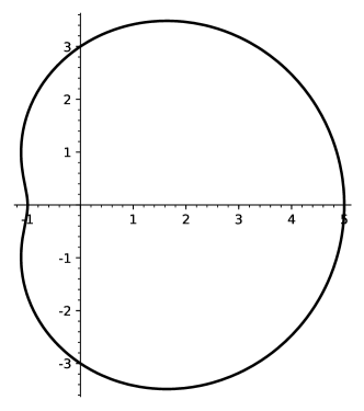
Figure 1. Non-algebraic image of the circle

According to Theorem 2.1, the set $p(\mathbb{T})$ can be completed to a real algebraic set by adding finitely many points, provided that $p$ is either an algebraic polynomial or a Laurent polynomial with $m<n$. The following example shows that the case $m=n$ is indeed exceptional.

Example 3.2.

Let $p(z)=z+z^{-1}$. Then $p(\mathbb{T})$ is the line segment $[-2,2]$. The smallest real algebraic set containing $p(\mathbb{T})$ is the real line $\mathbb{R}$.

The claimed properties of Example 3.2 are straightforward to verify. In addition, the polynomial $h$ from Theorem 2.1 can be computed as $h(x,y)=-4y^{2}$ which shows that $h$ is not necessarily irreducible.

4. Zero set of harmonic Laurent polynomials

The relation (2.5) highlights the importance of the zero set of the harmonic Laurent polynomial $P(z)=p(z)-p(1/\bar{z})$ where $p$ is a Laurent polynomial. It is not a trivial task to determine whether a given harmonic Laurent polynomial has unbounded zero set: e.g., Khavinson and Neumann [2] remarked on the varied nature of zero sets for rational harmonic functions in general. In this section we develop a necessary condition, in terms of the coefficients of $p$, for the function $P$ to have an unbounded zero set.

Suppose that $p$ is a Laurent polynomial (2.1) such that the associated function $P(z)=p(z)-p(1/\bar{z})$ has unbounded zero set. Consider the algebraic part of $P$, namely

(4.1) $$q(z)=\sum_{k=1}^{n}a_{k}z^{k}-\sum_{k=1}^{m}a_{-k}{\bar{z}}^{k}.$$

Then $q$ is a harmonic polynomial such that $\liminf_{z\to\infty}|q(z)|$ is finite. In other words, $q$ is not a proper map of the complex plane.

One necessary condition is immediate: if $m<n$, then $|q(z)|=a_{n}|z|^{n}+o(|z|^{n})$ as $z\to\infty$. Thus, $P$ can only have unbounded zero set if $m=n$.

We look for further conditions on a harmonic polynomial that ensure that it is a proper map of $\mathbb{R}^{2}$ to $\mathbb{R}^{2}$. More generally, given a polynomial map $F=(F_{1},\dots,F_{n})\colon\mathbb{R}^{n}\to\mathbb{R}^{n}$, let us decompose each component $F_{k}$ into homogeneous polynomials, and let $\mathcal{H}(F_{k})$ be the homogeneous term of highest degree in $F_{k}$. Write $\mathcal{H}(F)$ for $(\mathcal{H}(F_{1}),\dots,\mathcal{H}({F_{n}}))$, so that $\mathcal{H}(F)$ is also a polynomial map of $\mathbb{R}^{n}$. The following result is from [7], Lemma 10.1.9.

Lemma 4.1.

[L. Andrew Campbell] If $\mathcal{H}({F})$ does not vanish in $\mathbb{R}^{n}\setminus\{0\}$, then $F\colon\mathbb{R}^{n}\to\mathbb{R}^{n}$ is a proper map, that is $|F(x)|\to\infty$ as $|x|\to\infty$.

Lemma 4.1 can be restated in a form adapted to harmonic polynomials in $\mathbb{C}$.

Lemma 4.2.

Consider a harmonic polynomial $q(z)=\sum_{k=0}^{n}(a_{k}z^{k}+b_{k}\bar{z}^{k})$ of degree $n\geq 1$ as a map from $\mathbb{C}$ to $\mathbb{C}$.

1. If $|a_{n}|\neq|b_{n}|$, then $q$ is proper.

2. If $|a_{n}|=|b_{n}|$, let $\eta\in\mathbb{T}$ be such that $\eta a_{n}=\overline{\eta b_{n}}$. If $\eta a_{k}=\overline{\eta b_{k}}$ for $k=1,\dots,n$, then $q$ is not proper. Otherwise, let $K$ be the largest value of $k$ such that $\eta a_{k}\neq\overline{\eta b_{k}}$. If there is no $z\neq 0$ such that

   $$\operatorname{Re}(\eta a_{n}z^{n})=0=\operatorname{Im}((\eta a_{K}-\overline{\eta b_{K}})z^{K})$$

   then $q$ is proper.

Proof.

Part (a) follows from the reverse triangle inequality: $|q(z)|\geq\big{|}|a_{n}|-|b_{n}|\big{|}|z|^{n}+o(|z|^{n})$ as $n\to\infty$. To prove part (b), observe that

(4.2) $$\operatorname{Im}(\eta q(z))=\sum_{k=0}^{n}\operatorname{Im}((\eta a_{k}-\overline{\eta b_{k}}z^{k})$$

If $\eta a_{k}=\overline{\eta b_{k}}$ for $k=1,\dots,n$, then $\operatorname{Im}(\eta q)$ is constant, which means that up to a constant term, $\eta q$ is a real-valued harmonic function. By Harnack’s inequality, a nonconstant harmonic function $h\colon\mathbb{C}\to\mathbb{R}$ must be unbounded from above and from below, and therefore $q^{-1}(0)$ is an unbounded set. Since $q$ is constant on an unbounded set, it is not a proper map.

Finally, suppose that $K$, as defined in (b), exists. It follows from (4.2) that

$$\mathcal{H}(\operatorname{Im}(\eta q(z)))=\operatorname{Im}((\eta a_{K}-\overline{\eta b_{K}})z^{K})$$

Since also

$$\mathcal{H}(\operatorname{Re}(\eta p(z)))=\operatorname{Re}((\eta a_{n}+\overline{\eta b_{n}})z^{n})=2\operatorname{Re}(\eta a_{n}z^{n})$$

the last statement in (b) follows by applying Lemma 4.1 to $(\operatorname{Re}(\eta q),\operatorname{Im}(\eta q))$ considered as a map of $\mathbb{R}^{2}$ to $\mathbb{R}^{2}$. ∎

We are now ready to apply Lemma 4.2 to the special case $P(z)=p(z)-p(1/\bar{z})$ where $p$ is a Laurent polynomial. Recall that in view of Theorem 2.1 and the relation (2.5) the following result describes when the image $p(\mathbb{T})$ has infinite complement in the real algebraic set $V$ containing it.

Theorem 4.3.

Given a Laurent polynomial $p(z)=\sum_{k=-n}^{n}a_{k}z^{n}$ with $a_{n}a_{-n}\neq 0$, let $P(z)=p(z)-p(1/\bar{z})$. If the zero set of $P$ is unbounded, then one of the following holds:

1. $p(\mathbb{T})$ is contained in a line;

2. There exists $\eta\in\mathbb{T}$ such that $\eta a_{n}+\overline{\eta a_{-n}}=0$. Furthermore, there is an integer $k\in\{1,\dots,n-1\}$ such that the harmonic polynomial $\operatorname{Im}((\eta a_{k}+\overline{\eta a_{-k}})z^{k})$ is nonconstant and shares a nonzero root with the harmonic polynomial $\operatorname{Re}(\eta a_{n}z^{n})$.

As a partial converse: if (a) holds, then the zero set of $P$ is unbounded.

Although part (b) of Theorem 4.3 is convoluted, it is not difficult to check in practice because $\eta$ is uniquely determined (up to irrelevant sign) and the zero sets of both harmonic polynomials involved are simply unions of equally spaced lines through the origin.

Proof.

We apply Lemma 4.2 to the polynomial $q$ in (4.1), which means letting $b_{k}=-a_{-k}$ for $k=1,\dots,n$. Since $q$ is not proper, part (b) of the lemma provides two possible scenarios, which are considered below.

One possibility is that there exists a unimodular constant $\eta$ such that $\eta a_{k}=-\overline{\eta a_{-k}}$ for $k=1,\dots,n$. Therefore, for $z\in\mathbb{T}$ we have

$$\operatorname{Re}(\eta p(z))=\operatorname{Re}(a_{0})+\sum_{k=1}^{n}\left(re(\eta a_{k}z^{k}+\overline{\eta a_{-k}}z^{k}\right)=\operatorname{Re}(a_{0})$$

which means that $p(\mathbb{T})$ is contained in a line. The converse is true as well. If $p(\mathbb{T})$ is contained in a line, then there exists a unimodular constant $\eta$ such that $\operatorname{Re}(\eta p)$ is constant on $\mathbb{T}$. Considering the Fourier coefficients of $\operatorname{Re}(\eta p)$, we find $\eta a_{k}+\overline{\eta a_{-k}}=0$ for all $1\leq k\leq n$.

The other possibility described in Lemma 4.2 (b) transforms into part (b) of Theorem 4.3 with the substitution $b_{k}=-a_{-k}$. ∎

5. Intersection of polynomial images of the circle

As an application of Theorem 2.1, we establish an upper bound for the number of intersections between two images of the unit circle $\mathbb{T}$ under Laurent polynomials. It is necessary to exclude some pairs of polynomials from consideration, because, for example, the images of $\mathbb{T}$ under any two of the Laurent polynomials

$$p_{\alpha}(z)=z+z^{-1}+\alpha,\quad-2<\alpha<2,$$

have infinite intersection. This is detected by the computation of polynomial $h$ in Theorem 2.1, according to which $h(x,y)=-4y^{2}$ regardless of $\alpha$.

Theorem 5.1.

Consider two Laurent polynomials

$$p(z)=\sum_{k=-m}^{n}a_{k}z^{k}\quad\text{and}\quad\widetilde{p}(z)=\sum_{k=-r}^{s}b_{k}z^{k}$$

where $m,r\geq 0$, $n,s\geq 1$, and $a_{-m}a_{n}b_{-r}b_{s}\neq 0$. Then the intersection $p(\mathbb{T})\cap\widetilde{p}(\mathbb{T})$ consists of at most $4ns-2(n-m)(s-r)$ points unless the corresponding polynomials $h$ and $\tilde{h}$ from Theorem 2.1 have a nontrivial common factor.

In the special case of algebraic polynomials, $m=r=0$, the estimate in Theorem 5.1 simplifies to $2ns$. In this case the theorem is due to Quine [6, Theorem 3], where the bound $2ns$ is shown to be sharp. A related problem of counting the self-intersections of $p(\mathbb{T})$ was addressed in [5] for algebraic polynomials and in [3] for Laurent polynomials.

Proof.

Let $h_{\mathbb{C}}\in\mathbb{C}[w,\overline{w}]$ be the polynomial associated to $p$ by Theorem 2.1 (b). Consider its homogenization

$$H(w,\overline{w},\zeta)=\zeta^{2n}h_{\mathbb{C}}(w/\zeta,\overline{w}/\zeta).$$

Since $h_{\mathbb{C}}$ has degree $m+n$ in the variable $w$, it follows that $H$ has a zero of order at least $2n-(m+n)=n-m$ at the point $(1,0,0)$ of the projective space $\mathbb{C}\mathbb{P}^{2}$. Similarly, it has a zero of order at least $n-m$ at the point $(0,1,0)$.

The homogeneous polynomial $\widetilde{H}$ associated with $\widetilde{p}$ has zeros of order at least $s-r$ at the same two points. Therefore, the projective curves $H=0$ and $\widetilde{H}=0$ intersect with multiplicity at least $(n-m)(s-r)$ at each of the points $(1,0,0)$ and $(0,1,0)$ (Theorem 5.10 in [8, p. 114]).

Bezout’s theorem implies that, unless $H$ and $\widetilde{H}$ have a nontrivial common factor, the projective curves $H=0$ and $\widetilde{H}=0$ have at most $\deg H\deg\widetilde{H}=4ns$ intersections in $\mathbb{C}\mathbb{P}^{2}$, counted with multiplicity. Subtracting the intersections at two aforementioned points, we are left with at most $4ns-2(n-m)(s-r)$ points of intersection in the affine plane. ∎

References

- [1] Pavel M. Bleher, Youkow Homma, Lyndon L. Ji, and Roland K. W. Roeder, Counting zeros of harmonic rational functions and its application to gravitational lensing, Int. Math. Res. Not. IMRN 2014 (2014), no. 8, 2245–2264.
- [2] Dmitry Khavinson and Genevra Neumann, On the number of zeros of certain rational harmonic functions, Proc. Amer. Math. Soc. 134 (2006), no. 4, 1077–1085.
- [3] Leonid V. Kovalev and Sergei Kalmykov, Self-intersections of laurent polynomials and the density of jordan curves, Proc. Amer. Math. Soc. (2019), to appear. Available at arXiv:1902.02468.
- [4] Grace Orzech and Morris Orzech, Plane algebraic curves, Monographs and Textbooks in Pure and Applied Math., vol. 61, Marcel Dekker, Inc., New York, 1981, An introduction via valuations.
- [5] J. R. Quine, On the self-intersections of the image of the unit circle under a polynomial mapping, Proc. Amer. Math. Soc. 39 (1973), 135–140.
- [6] by same author, Some consequences of the algebraic nature of , Trans. Amer. Math. Soc. 224 (1976), no. 2, 437–442 (1977).
- [7] Arno van den Essen, Polynomial automorphisms and the Jacobian conjecture, Progress in Mathematics, vol. 190, Birkhäuser Verlag, Basel, 2000.
- [8] Robert J. Walker, Algebraic curves, Springer-Verlag, New York-Heidelberg, 1978, Reprint of the 1950 edition.
- [9] Hassler Whitney, Elementary structure of real algebraic varieties, Ann. of Math. (2) 66 (1957), 545–556.
- [10] A. S. Wilmshurst, The valence of harmonic polynomials, Proc. Amer. Math. Soc. 126 (1998), no. 7, 2077–2081.