Deep Learning Architectures for Automated Image Segmentation

Abstract

Image segmentation is widely used in a variety of computer vision tasks, such as object localization and recognition, boundary detection, and medical imaging. This thesis proposes deep learning architectures to improve automatic object localization and boundary delineation for salient object segmentation in natural images and for 2D medical image segmentation.

First, we propose and evaluate a novel dilated dense encoder-decoder architecture with a custom dilated spatial pyramid pooling block to accurately localize and delineate boundaries for salient object segmentation. The dilation offers better spatial understanding and the dense connectivity preserves features learned at shallower levels of the network for better localization. Tested on three publicly available datasets, our architecture outperforms the state-of-the-art for one and is very competitive on the other two.

Second, we propose and evaluate a custom 2D dilated dense UNet architecture for accurate lesion localization and segmentation in medical images. This architecture can be utilized as a stand alone segmentation framework or used as a rich feature extracting backbone to aid other models in medical image segmentation. Our architecture outperforms all baseline models for accurate lesion localization and segmentation on a new dataset. We furthermore explore the main considerations that should be taken into account for 3D medical image segmentation, among them preprocessing techniques and specialized loss functions.

Computer Science 2019 Demetri Terzopoulos Song-Chun Zhu Fabien Scalzo To my mother, Chandana Sengupta, and my father, Dipanjan Sengupta, for their unconditional love and support and for always inspiring me to be the best version of myself.

Chapter 0 Introduction

Figure 1: (a) Example of natural image (left) and its corresponding salient object map (right). (b) Example of 2D brain MRI (left) and the corresponding lesion segmentation map (right). (c)Example of 3D liver CT from top, side and front perspectives (left) and corresponding liver segmentation maps for top, side and front perspectives (right). Liver is highlighted in red on the original CT (left).

Image segmentation is a prominent concept of computer vision. It is the process of partitioning the pixels of an image into “segments” associated with different classes. The main goal of segmentation is often to simplify the representation of an image such that it is easier to interpret, analyze, and understand. Image segmentation has been used in a variety of computer vision tasks, such as object localization, boundary detection, medical imaging, and recognition. In essence, these tasks are performed by assigning each pixel in an image to a certain label based on similar attributes, such as texture, color, intensity, or distance metrics. The result of image segmentation is a set of segments that collectively cover the entirety of an image. The focus of this thesis is to develop novel deep learning methods for the segmentation of natural images and of 2D and 3D medical images. Deep learning is a form of machine learning that employs artificial neural network architectures with many hidden layers (Hinton et al., 2012).

Specifically, we consider two types of segmentation. The first is salient object segmentation. On natural images, it involves the detection of the most prominent, noticeable, or important object within the image. In image understanding, a saliency map classifies each pixel in the image as part of the salient object or as part of the background. Figure 1a illustrates an example of an image and its associated saliency map. Salient object segmentation is especially important because it focuses attention on the most important aspects of an image. An example use case is smart image cropping and resizing, where the image is automatically cropped without losing the most salient imaged objects. Another use case is in UI/UX design (Kurtulmus, 2017), where salient object segmentation is used to understand what parts of a user interface are most useful, thus assisting in the development of even better user interfaces for a smoother user experience. By helping automate the process of determining the most important parts of images, salient object segmentation supports a number of other product pipelines.

The second type of segmentation that we consider is medical image segmentation. Accurate medical image segmentation is often the first step in a diagnostic analysis of the patient and, therefore, a key step in treatment planning (Aggarwal et al., 2011). An important topic in medical image segmentation is the automatic delineation of anatomical structures in 2D or 3D medical images. In our work, we use binary medical image segmentation to detect lesions in 2D MR scans and CT scans of the brain and lung, and swollen lymph nodes in 3D CT scans. The goal, whether for 2D or 3D images, is to create a model that can accurately segment a lesion, organ, or cancerous region in a CT or MR scan. Figure 1b and c shows examples of lesion segmentation in 2D and 3D images. Deep learning approaches to medical image segmentation raise many challenges not faced in salient object detection on natural images. Some examples are the lack of large training datasets, specialized preprocessing techniques on different medical imaging modalities, memory constraints with 3D medical images, and the inability to use priors on the shapes of lesions because they are unique to each patient.

Traditionally, active contour models were broadly applied to the task of image segmentation (Kass et al., 1988; Zhu and Yuille, 1996; Osher and Fedkiw, 2001). These models rely on the content of the image and minimize an energy functional associated with deformable contours that delineate the segmentation process. In recent years, with ever-increasing computational power from GPUs and the availability of more plentiful training data, deep convolutional neural networks have achieved state-of-the-art performance on benchmark datasets in various image recognition tasks (Krizhevsky et al., 2012; Simonyan and Zisserman, 2014; He et al., 2016). Image segmentation has also benefited from various fully convolutional architectures (Badrinarayanan et al., 2015), notably encoder-decoder architectures such as UNet (Ronneberger et al., 2015).

1 Contributions

Although deep-learning assisted models for image segmentation have achieved acceptable results in many domains, these models are yet incapable of producing segmentation outputs with precise object boundaries. This thesis aims to advance the current paradigm by proposing and evaluating novel architectures for the improved delineation of object boundaries in images.

We first tackle the problem of salient object detection and segmentation in natural images and propose an effective architecture for localizing objects of interest and delineating their boundaries. We then investigate the problem of cancerous lesion segmentation and address the aforementioned issues in various 2D medical imaging datasets that contain lesions of different sizes and shapes. Finally, we explore the preprocessing considerations that should be taken into account when transitioning from 2D segmentation models to 3D. We evaluate these considerations by preprocessing an abdominal lymph node dataset. We then train and fine-tune a 3D VNet model using the preprocessed dataset.

In addition to the suitability of the proposed architectures as standalone models, they can also be leveraged in an integrated framework with energy-based segmentation components to decrease the dependence on external inputs as well as improve robustness. In particular, the concepts and 2D architectures developed in this thesis (Chapters 3 and 4) were used as a backbone in integrated frameworks for International Conference on Machine Learning (ICML) 2019, Conference on Computer Vision and Pattern Recognition (CVPR) 2019 (Hatamizadeh et al., 2019a),International Conference on Computer Vision (ICCV) 2019 (Hatamizadeh et al., 2019d) and Machine Learning in Medical Imaging (MLMI) workshop for MICCAI (accepted) (Hatamizadeh et al., 2019b).

2 Overview

The remainder of this thesis is organized as follows:

• Chapter 2 reviews related work. We first discuss image segmentation techniques that were popular prior to deep learning methods. The transition to deep learning segmentation methods is then highlighted. Finally, three deep learning architectures that inspired our work are discussed in detail; namely, UNet, DenseNet, and VNet.

• Chapter 3 introduces a novel deep neural network architecture for the task of salient object segmentation. Its features include, an encoder-decoder architecture with dense blocks and a novel dilated spatial pyramid pooling unit for better spatial image understanding.

• Chapter 4 explores a more specific use case for image segmentation—medical image segmentation. We introduce a novel deep learning architecture for 2D medical image segmentation on a new medical image dataset from Stanford University. The highlights of this architecture are an encoder-decoder network with dense blocks that performs competitively with the state-of-the-art architectures, yet with very limited training data.

• Chapter 5 discusses important considerations required to transition from a 2D segmentation model to a 3D segmentation model. The importance of preprocessing techniques in the 3D case is highlighted. A 3D medical dataset is preprocessed using these techniques and a 3D VNet is trained and fine-tuned with the processed data.

• Chapter 6 presents our conclusions and proposes future work.

Chapter 1 Related Work

This chapter first reviews segmentation techniques that have been explored prior to the rise of deep learning for segmentation. Then, we review three noteworthy deep learning architectures that have inspired our work, namely UNet, DenseNet, and VNet.

1 Salient Object Segmentation

Salient object segmentation is the task of detecting the most prominent object in an image and classifying each image pixel as either part of that object or part of the background (a binary classification task). Prior to deep learning methods, there were five main categories of salient image segmentation methods, namely region-based methods, classification methods, clustering methods, and hybrid methods, as discussed by Norouzi et al. (2014), as well as active contour models. For each method, we will describe the algorithm, followed by its advantages and disadvantages.

There are two main region-based methods, thresholding and region growing. Thresholding (Bogue, 2005) is a simple segmentation approach that divides the image into different segments based on different thresholds of pixel intensity. In other words, this method assumes that, given an image, all pixels belonging to the same object have similar intensities, and that the overall intensities of different objects differ. Global thresholding assumes that the pixel distribution of the image is bimodal. In other words, there is a clear difference in intensity between background and foreground pixels. However, this naive, global method performs very poorly if the image has significant noise and low variability in inter-region pixel intensity. More sophisticated global thresholding techniques include Otsu’s Thresholding (Qu and Zhang, 2010). This method assumes a two-pixel class image in which the threshold value aims to minimize the intra-class variance. Local thresholding helps this issue by dividing images into subimages, determining a threshold value for each subimage, and combining them to obtain the final segmentation. Local thresholding is achieved using different statistical techniques, including calculating the mean, standard deviation, or maximum/minimum of a subregion. An even more sophisticated method of thresholding is region growing. This method requires an initial seed that grows due to similar properties for surrounding pixels, representing an object, as done by Leung and Malik (1998). The obvious drawback to this approach is that it is heavily dependent on the selection of the seeds by a human user. Human interaction often results in a high chance of error and differing results from different users.

K-nearest neighbors and maximum likelihood are simple classification methods that were prominent prior to deep learning. For each image, pixels are assigned to different object classes based on classification learned at training time. The advantage of maximum likelihood classification is that it is easy to train. Its disadvantage is that it often requires large training sets. Clustering methods attempt to mitigate the issues faced with classification since they do not require a training set. They use statistical analysis to understand the distribution and representation of the data and, therefore, are considered unsupervised learning approaches. Some examples of clustering include, k-means, fuzzy C-mean, and expectation maximization (Ma et al., 2009). The main disadvantage of clustering methods is that they are sensitive to noise since they do not take into account the spatial information of the data, but only cluster locally.

Hybrid methods are techniques that use both boundary (thresholding) and regional (classification/clustering) information to perform segmentation. Since this method combines the strengths of region-based, classification, and clustering methods, it has proven to give competitive results among the non-deep-learning techniques. One of the most popular methods is the graph-cut method. This method requires a user to select initial seed pixels belonging to the object and to the background. Then, it uses the minimum cut algorithm on the graph generated from the image pixels, as discussed by Boykov and Jolly (2001). The drawback is the need for a user to select the initial seeds. This is error prone for low contrast images and would be more advantageous if it could be automated.

Active contour models (ACMs), introduced by Kass et al. (1988) have been very popular for segmentation, as in (Vese and Chan, 2002), and for object boundary detection, as in (Mishra et al., 2011). Active contour models utilize formulations in which an initial contour evolves towards the object’s boundary via the minimization of an energy functional. Level set ACMs can handle large variations in shape, image noise, heterogeneity, and discontinuous object boundaries, as shown by Li et al. (2011). This method is extremely effective if the initialization of the contours and weighted parameters is done properly. Researchers have proposed automatic initialization methods, such as using shape priors or clustering methods. Although they eliminate a manual initialization step, techniques such as shape priors require representative training data.

For the task of salient object detection, we work with natural images, which offers certain advantages when compared to working with medical images. Much larger datasets of natural images are available and the use of priors is possible, since the shapes of basic objects such as animals, furniture, or cars, are known. Prior models were used by Han et al. (2015) who proposed a framework for salient object detection by first modeling the background and then separating salient objects from the background.

2 2D and 3D Medical Image Segmentation

Modern technology has enabled the production of high quality medical images that aid doctors in illness diagnosis. There are now several common image modalities such as MR, CT, X-ray, and others. Medical image segmentation is often the first step in a diagnosis analysis plan. Aggarwal et al. (2011) explain that accurate segmentation is a key step in treatment planning. Such images are often segmented into organs or lesions within organs. Before the advent of computer vision in medical image analysis, segmentations were often done manually, with medical technicians manually tracing the boundaries of different organs and lesions. This process is not only tedious for technicians but also error prone, since tracing accurate boundaries by hand can be rather tricky in some cases.

In the past few decades, many effective algorithms have been developed to aid the segmentation process (Ma et al., 2009). The methods reviewed in the previous section have been applied to medical image segmentation. However, in the medical domain, copious quantities of labeled training data are rare, therefore clustering methods like k-means, which was first applied to medical images by Korn et al. (1996), often do not prove to be robust. Furthermore, obtaining priors for active contour models is sometimes possible but is oftentimes difficult in the medical imaging domain. In lesion segmentation, for example, not only is data limited, but every lesion is unique to a given patient; therefore, it is difficult to obtain a prior model for lesions. In order to use the techniques mentioned in the previous section, researchers would heavily depend on data augmentation, something that is still common with deep learning models.

The rise of deep learning techniques in computer vision has been momentous in the recent past. The first to propose a fully convolutional deep neural network architecture for semantic segmentation was Long et al. (2015). Deep learning is now being heavily used in medical image segmentation due to its ability to learn and extract features on its own, without the need for hand-crafting features or priors. Convolutional and pooling layers are used to learn the semantic and appearance information and produce pixel-wise prediction maps. This work enabled predictions on input images of arbitrary sizes. However, the predicted object boundaries are often blurred due to the loss of resolution due to pooling. To mitigate the issue of reduced resolution, Badrinarayanan et al. (2015) proposed an encoder-decoder architecture that maps the learned low-resolution encoder feature maps to the original input resolution. Adding onto this encoder-decoder approach, Yu and Koltun (2015) proposed an architecture that uses dilated convolutions to increase the receptive field in an efficient manner while aggregating multi-scale semantic information. Ronneberger et al. (2015) proposed adding skip connections at different resolutions. In recent years, many 2D and 3D deep learning architectures for segmentation have demonstrated promising results (Hatamizadeh et al., 2018, 2019e; Myronenko and Hatamizadeh, 2019; Hatamizadeh et al., 2019c).

3 Deep Learning Architectures

In this section, the three architectures that inspired the deep learning models developed in Chapter 3, 4 and 5 are discussed in greater detail.

1 UNet

The UNet architecture introduced by Ronneberger et al. (2015) was one of the first convolutional networks designed specifically for biomedical image analysis. This network aimed to tackle two issues that are specific to the domain in medical image segmentation. The first is the lack of large datasets in this domain. The goal of this architecture is to produce competitive segmentation results given a relatively small quantity of training data. Traditional feed-forward convolutional neural networks with fully connected layers at the end have a large number of parameters to learn, hence require large datasets. These models have the luxury of learning little bits of information over a vast number of examples. In the case of medical image segmentation, the model needs to maximize the information learned from each example. Encoder-decoder architectures such as UNet have proven to be more effective even with small datasets, because the fully-connected layer is replaced with a series of up convolutions on the decoder side, which still has learnable parameters, but much fewer than a fully-connected layer. The second issue the UNet architecture tackles is to accurately capture context and localize lesions at different scales and resolutions.

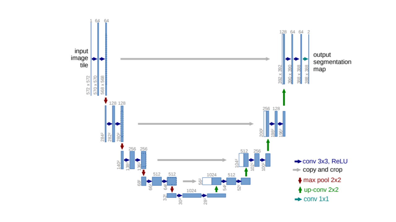
Figure 1: Original UNet architecture from Ronneberger et al. (2015)

Architecture Details:

The UNet architecture consists of two portions, as shown in Figure 1. The left side is a contracting path, in which successive convolutions are used to increase resolutions and learn features. The right side is an expanding path of a series of upsampling operations. Low resolution features from the contracting path are combined with upsampled outputs from the expanding path. This is done via skip connections and is significant in helping gain spatial context that may have been lost while going through successive convolutions on the contracting path. The upsampling path utilizes a large number of feature channels, which enables the effective propagation of context information to lower resolution layers on the contracting path, allowing for more precise localization. This motivated the authors to make the expanding path symmetric to the contracting path, forming a U-shaped architecture.

The authors also mention another noteworthy issue faced for medical image segmentation, namely the problem of objects of the same class touching each other with fused boundaries. To alleviated this issue, they propose using a weighted loss by separating background labels between touching segments to contribute to a large weight in the loss function.

Training:

The UNet model is trained with input images and their corresponding segmentation maps via stochastic gradient descent. The authors utilize a pixel-wise softmax function over the final segmentation and combine it with a cross-entropy loss function. Weight initialization is important to help control regions with excessive activation that over contribute to learning the correct weight parameters and ignoring other regions. Ronneberger et al. (2015) recommend initializing the weights for each feature maps so that the network has unit variance. To achieve this for the UNet architecture, they recommend drawing the initial weights from a Gaussian distribution. The authors also discuss the importance of data augmentation since medical image datasets are often small. Techniques such as shifting, rotating, and adding noise are most popular for medical images.

The success of the UNet architecture makes it very appealing to explore and build upon for different medical segmentation tasks. Ronneberger et al. (2015) demonstrated the success of this model on a cell segmentation task. We will take this architecture as a baseline for our work on lesion segmentation in the brain and lung in Chapter 4.

2 DenseNet

The DenseNet architecture was introduced by Huang et al. (2016). Although this architecture was not designed specifically for application to medical image segmentation, the ideas can be effectively applied to the medical imaging domain.

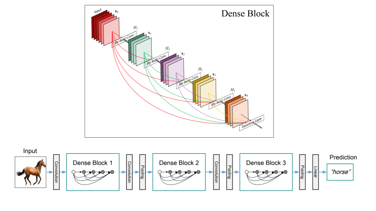
Figure 2: Original DenseNet architecture from Huang et al. (2016). The top figure depcits an example dense block. The bottom figure depicts a full DenseNet architecture.

Architecture Details:

DenseNet, depicted in Figure 2, is a deep network that connects each layer to every other layer. This architecture extends on the observations that deep convolutional networks are faster to train and perform better if there are shorter connections between input and output layers. Therefore, each layer takes the feature maps generated from all preceding layers and the current feature maps as input for all successive layers. Interestingly enough, there are actually fewer parameters to learn in this architecture than in architectures such as ResNet, proposed by He et al. (2016), because it avoids learning redundant information. Instead, each layer takes what has already been learned before as input. In addition to efficient parameter learning, the backpropagation of gradients is much smoother. Each layer has access to the gradients from the loss function and the original input signal, leading to an implicit deep supervision. This also contributes to natural regularization, which is beneficial for small datasets where overfitting is often an issue.

As mentioned previously, a goal of DenseNet is to improve information flow for fast and efficient backpropagation. For comparison, consider how information flows through an architecture such as ResNet. In a traditional feedforward convolutional network, each transition layer is described as $x_{l}=Z_{l}(x_{x-1})$, where $Z$ is a composite of convolution, batch norm, and ReLU operations. ResNet also has a residual connection to the previous layer. The composite function is

$$x_{l}=Z_{l}(x_{x-1})+x_{l-1}.$$ (1)

Although the connection to the previous layer assists in gradient flow, the summation makes gradient flow somewhat slow. To combat this issue, DenseNet uses concatenation instead of summation for information flow:

$$x_{l}=Z_{l}([x_{l-1};x_{l-2};\dots;x_{0}]),$$ (2)

where $[a;b;c]$ denotes concatenation. This idea is referred to as dense connectivity. DenseNet is a collection of such dense blocks with intermediate convolution and pooling layers, as shown in Figure 2.

The main points of success for this model is that there is no redundancy in learning parameters and the concatenation of all prior feature maps makes gradient backpropagation more efficient to assist in faster learning. Ideas from DenseNet have inspired the work in Chapters 3 and 4.

3 VNet

The VNet architecture was introduced by Milletari et al. (2016). It is very similar to that of the UNet, as shown in Figure 3. The motivation for this architecture was that much of medical image data is 3D, but most deep learning models at the time seemed to focus on 2D medical image segmentation. Therefore, the authors developed an end-to-end 3D image segmentation framework tailored for 3D medical images.

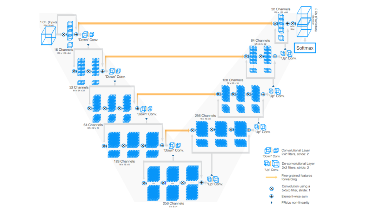
Figure 3: Original VNet architecture from Milletari et al. (2016).

Architecture Details:

The VNet architecture consists of a compression path on the left, which reduces resolution, and an expansion path on the right, which brings the image back to its original dimensions, as shown in Figure 3. On the compression path, convolutions are performed to extract image features, and at the end of each stage, reduce the image resolution before continuing to the next stage. On the decompression path the signal is decompressed and the original image dimensions are restored.

The main difference between the VNet and the UNet lies in the operations applied at each stage. In a conventional UNet, as shown in Figure 1, at each stage, the compression path performs convolutions to extract features at a given resolution and then reduces the resolution. The VNet does the same, but the input of each stage is used in the convolutional layers of that stage and it is also added to the output of the last convolutional layer of that stage. This is done to enable the learning of a residual function; hence, residual connections are added in each stage. Milletari et al. (2016) observed that learning a residual function cuts the convergence times significantly, because the gradient can flow directly from the output of each stage to the input via residual connections during backpropagation.

Another notable difference between the VNet and the UNet is the technique used to reduce resolutions between stages. In the case of the UNet, after an input goes through convolutions and a nonlinearity, it is fed into a max pool layer to reduce resolution. In the case of the VNet, after the nonlinearity, the input is fed through a convolution with a $2\times 2\times 2$ voxel-wide kernel applied with a stride of length 2. As a result, the size of the feature maps is halved before proceeding to the next stage. This strategy is more memory efficient, which is highly advantageous since memory scarcity is a big problem for most 3D models.

The expansion portion of the VNet extracts features and enables the spatial understanding from low resolution feature maps in order to build a final volumetric segmentation. After each stage of the expansion path, a deconvolution operation is applied to double the size of the input, until the original image dimensions are restored. The final feature maps are passed through a softmax layer to obtain a probability map predicting whether each voxel belongs to the background or foreground. Residual functions are also applied on the expansion path.

The main point of success for this model is that it was the first effective and efficient end-to-end framework for 3D image segmentation. It utilized an encoder-decoder scheme with learned residual functions, resulting in faster convergence than other 3D networks. It employs convolutions for resolution reduction instead of using a max pooling layer, which is more memory efficient, a very important point for 3D architectures. VNet and its variants have proven to be very promising in a variety of 3D segmentation tasks, such as multi-organ abdominal segmentation (Gibson et al., 2018) and pulmonary lobe segmentation (Hatamizadeh et al., 2018). This architecture will be further explored in Chapter 5.

Chapter 2 2D Natural Image Segmentation

The manual delineation of segmentation boundaries is an error-prone procedure that is cumbersome, time intensive, and subject to user variability. Deep learning methods automate delineation by having learned parameters detect boundaries. This chapter discusses the implementation of a series of deep learning models to improve object delineation of boundaries in the task of salient object segmentation in natural images; i.e., images of everyday “natural” objects.

Encoder-decoder architectures have proven to be very effective in tasks such as semantic segmentation; however, they are yet to be heavily explored for use in salient object detection. To this end, we propose a custom dense encoder-decoder with depthwise separable convolution and dilated spatial pyramid pooling. This is a simple and effective method to assist in object localization and boundary detection with spatial understanding.

The custom encoder-decoder architecture, as depicted in Figure 2, is tailored to estimate a binary segmentation map with accurate object boundaries. In this architecture, the encoder increases the size of the receptive field while decreasing the spatial resolution by a series of successive dense blocks. The decoder employs a series of transpose convolutions and concatenations via skip connections with high-resolution extracted features from the encoder.

The novelty in our architecture is that we create a light, custom dilated spatial pyramid pooling (DSPP) block at the end of the encoder. The output of the encoder is fed into 4 parallel dilation channels and the results are concatenated before passing it to the decoder, as shown in Figure 2. Since there are various features in natural images, such as scale and resolution, we utilized a dilated spatial pyramid pooling block to restore the spatial information that may have been lost while reducing resolutions on the encoder side for more accurate boundary detection of the salient object.

The following sections systematically go through a series of architectures before arriving at the implementation for the novel dense encoder-decoder with dilated pyramid pooling. The final architecture is validated on three prominent publicly available datasets used for the task of salient object detection, namely MSRA, ECSSD, and HKU.

1 Basic Encoder Decoder

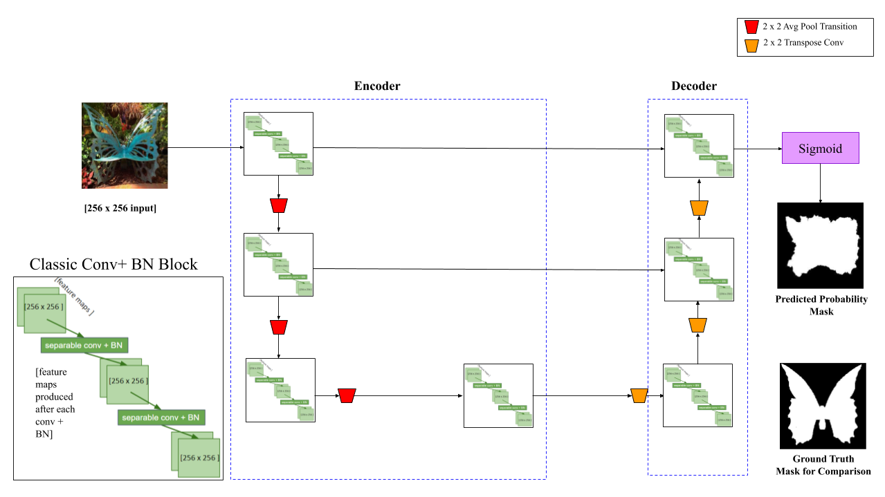
Figure 1: Basic Encoder-Decoder Model. The basic encoder-decoder model, a classic convolution + batch norm block and the associated produced feature maps are depicted.

We first explore a basic encoder-decoder architecture, illustrated in Figure 1, for the task of salient object detection.

1 Implementation

In the encoder portion, the number of learned feature maps is incrementally increased by powers of two, from 64 filters to 1024 filters. The size of the image is decreased by half at each stage of the encoder. The end of the encoder samples at the lowest resolution to capture high-level features regarding the object shapes. In the decoder portion, the number of feature maps is decreased by powers of two, from 1024 to 64. The image dimensions are restored to the input dimensions, by doubling at each stage. We pass the last layer through a sigmoid filter to produce the final binary map.

Preprocessing:

For this task, the original input image sizes are $300\times 400$. The input images are resized to $256\times 256$. This is done because 256 is the best value to minimize distortion but still make the data uniform to feed into the network.

Convolution:

The basic encoder-decoder architecture utilizes depthwise separable convolution. Each depthwise separable convolutional layer in the proposed architecture may be formulated as follows:

$$c_{\mathrm{separable}}(X,W,\gamma)=r(b(X*W),\gamma).$$ (1)

It consists of an input $X$, a learned kernel $W$, a batch normalization $b$, and a ReLU unit $r(X)=\max(0,X)$. Depthwise separable convolution is used because it is a powerful operation that reduces the computational cost and number of learned parameters while maintaining similar performance to classic convolutions. Classic convolutions are factorized into depthwise spatial convolutions over individual channels and pointwise convolutions, and combines the results of convolutions over all channels.

2 Results and Analysis

dataset	$F_{\beta}$	MAE
ECSSD	0.737	0.120
MSRA	0.805	0.093
HKU	0.804	0.079

Table 1: $F_{\beta}$ and MAE scores for basic encoder-decoder model on the ECSSD, MSRA, and HKU datasets.

As shown in Table 1, a basic encoder-decoder structure alone has mediocre performance. Reasons for this could include that as an image goes deeper into the encoder, the model loses information learned directly from higher resolutions. As a result, the model is able to correctly localize the object but is unable to predict accurate image boundaries. This was especially observed when an image had multiple objects with more complex boundaries. In the next section, dense blocks are added to the encoder portion to mitigate this issue.

2 Dilated Dense Encoder-Decoder

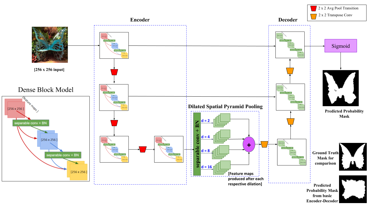
Figure 2: Dilated Dense Encoder-Decoder with Dilated Spacial Pyramid Pooling. Dilated Dense Encoder-Decoder with Dilated Spacial Pyramid Pooling (DSPP) Block is depicted. Inside the DSPP, the output of the encoder is fed into 4 parallel dilations to increase the receptive fields at different scales, depicted in blue text.

The main differences between the basic encoder-decoder implementation and the custom encoder-decoder discussed in this section, are as follows:

• Implementing dense block units

• Implementing a custom dilated spacial pyramid pooling block

As shown in Figure 2, in addition to using depthwise separable convolutions, the basic convolutional blocks are replaced with dense blocks, as employed by Huang et al. (2016). The advantage of utilizing dense blocks is that each dense block takes as input the information from all previous layers. Therefore, at deeper layers of the network, information learned at shallower layers is not lost. A custom dilated spatial pyramid pooling block is added at the end of the encoder for better spatial understanding, as illustrated in Figure 2.

In this dilated dense encoder-decoder model, the encoder portion increases the receptive field while decreasing the spatial resolution by a series of successive dense blocks, instead of by convolution and pooling operations in typical UNet architectures. The bottom of the dilated dense encoder-decoder consists of convolutions with dilation to increase the spatial resolution for better image understanding. The decoder portion employs a series of up-convolutions and concatenations with high-resolution extracted features from the encoder in order to gain better localization and boundary detection. The dilated dense encoder-decoder was designed to allow lower-level features to be extracted from 2D input images and passed to the higher levels via dense connectivity for more robust image segmentation.

1 Implementation

In each dense block, depicted in Figure 2, a composite function of depthwise separable convolution, batch normalization, and ReLU, is applied to the concatenation of all the feature maps $[x_{0},x_{1},\dots,x_{l-1}]$ from layers 0 to $l-1$. The number of feature maps produced by each dense block is $k+n\times k$, where each layer in the dense block contributes $k$ feature maps to the global state of the architecture and each block has $n$ intermediate layers (the $n\times k$ term), plus the $k$ layers that comprise the transition layer at the end of the dense block (the $k$ term).

We observed that a moderately small growth rate of $k=12$ sufficed to learn decent segmentation, allowing us to increase the model’s learning scope with dense blocks. The tradeoff between better learning via more parameters and still keeping the model relatively efficient, using a smaller value of $k$, was a consideration during model tuning for fast convergence. One reason for the success of a smaller growth rate is that each layer has information about all subsequent layers and has knowledge of the global state (Huang et al., 2016). $k$ regulates the amount of new information that is added to the global state at each layer. This means that any layer in the network has information regarding the global state of the entire network. Thus it is unnecessary to replicate this information layer-to-layer and a small $k$ suffices.

Dilated Spatial Pyramid Pooling:

Dilated convolutions make use of sparse convolution kernels to represent functions with large receptive fields and with the advantage of few training parameters. Dilation is added to the bottom of the encoder-decoder structure, as shown in Figure 2. Assuming that the last block of the encoder is $x$, and letting $D(x,d)$ represent the combined batch norm-convolution-reLU function, with dilation $d$ on input $x$, the dilation may be written as

$$Y=[D(x,2);D(x,4);D(x,8);D(x,16)],$$ (2)

where $[D();D()]$ represents concatenations. The last dense block is fed into 4 parallel convolutional layers with dilation 2, 4, 8, and 16. Once the blocks go through function $D$, they are concatenated to gain wider receptive fields and spatial perspective at the end of the encoder. This is only done at the bottom of the architecture because it is the section with the least resolution, the “deepest” part of the network. This allows for an expanded spatial context before continuing into the decoder path.

2 Results and Analysis

dataset	$F_{\beta}$	MAE
ECSSD	0.825	078
MSRA	0.857	0.061
HKU	0.845	0.087

Table 2: $F_{\beta}$ and MAE Score for dilated dense encoder-decoder on the ECSSD, MSRA, and HKU datasets.

Table 2 shows the results of the dilated dense encoder-decoder model with dilated spatial pyramid pooling. We observed that this architecture performed significantly better than the basic encoder-decoder architecture (Table 1).

Model	ECSSD ($F_{\beta}$)	ECSSD (MAE)	MSRA ($F_{\beta}$)	MSRA (MAE)	HKU ($F_{\beta}$)	HKU (MAE)
MC Zhao et al. (2015)	0.822	0.107	0.872	0.062	0.781	0.098
MDF Li and Yu (2015)	0.833	0.108	0.885	0.104	0.860	0.129
ELD Lee et al. (2016)	0.865	0.981	0.914	0.042	0.844	0.071
ED Ronneberger et al. (2015)	0.737	0.120	0.805	0.093	0.804	0.079
DDED	0.825	0.078	0.857	0.061	0.845	0.087
DDED + ACL	0.920	0.048	0.881	0.046	0.861	0.054
SOA Hou et al. (2017)	0.915	0.052	0.927	0.028	0.913	0.039

Table 3: Model Evaluations. $F_{\beta}$ and MAE values for each model on ECSSD, MSRA, and HKU datasets. ED abbreviates encoder-decoder. DDED abbreviates dilated dense encoder-decoder. ACL abbreviates active contour layer.

This network was the backbone CNN used in the full pipeline proposed in our ICML 2019 submission. The results are presented in Table 3. DDED indicates results from the stand-alone dilated dense encoder-decoder, described in this section. ED indicates the results from the basic encoder-decoder described in the previous section.

The full pipeline consisted of the DDED backbone CNN and an active contour layer (ACL). The output of the dilated dense encoder-decoder is taken as input into the ACL, which then produces the final segmentation results, seen in (DDED + ACL). As observed in Table 3, the DDED + ACL architecture beats the current state-of-the-art for the ECSSD dataset and is competitive with the state-of-the-art for the MSRA and HKU datasets. The ECSSD dataset contained many images with highly complex boundaries. The full DDED + ACL framework accurately delineates object boundaries, resulting in an increased $F_{\beta}$ score for the ECSSD dataset. This demonstrates the strength of this framework, in which the backbone DDED was trained from random initialization but yielded competitive results, in comparison to other models (MC, MDF, ELD) that utilized pre-trained CNN backbones, such as ImageNet (Deng et al., 2009), AlexNet (Krizhevsky et al., 2012), GoogLeNet (Szegedy et al., 2015) and OverFeat (Sermanet et al., 2013).

Figure 3 illustrates the performance of the ED, DDED, and DDED + ACL frameworks for precise boundary delineation. The images are grouped into categories highlighting different characteristics of the images. The grouping is utilized to indicate the success of the DDED and the DDED + ACL frameworks in a variety of cases. It is observe that all of the images from the dilated dense encoder-decoder (d), are much closer to the ground truth (b) than the results from basic encoder-decoder (e). Therefore (d) proves to be a very robust backbone architecture for this segmentation pipeline, which is required for accurate boundary detection of the ACL. The results in (d) also indicate that the dilated dense encoder-decoder model can also be a successful stand alone model, as almost all images produced are very close to the ground truth (b).

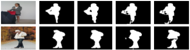
(a) Simple Scene $|$ Center Bias

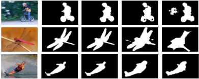
(b) Large Object $|$ Complex Boundary

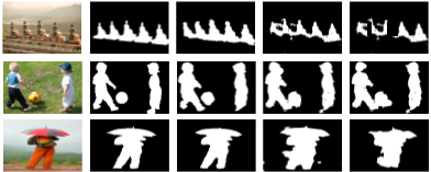
(c) Low Contrast $|$ Complex Boundary

(d) Large Object $|$ Complex Boundary $|$ Center Bias

Figure 3: Examples of Segmentation Outputs. (a) Original image. (b) Ground truth. (c) DDED + ACL output segmentation. (d) DDED output segmentation. (e) ED output segmentation.

3 Loss Function

The Dice coefficient is utilized as the loss function, which is defined as

$$\mathrm{Loss}=1-\frac{2\times|X\cap Y|}{|X|+|Y|},$$ (3)

where $X$ is the prediction matrix, $Y$ is the ground truth matrix, $|X|$ is the carnality of the set $X$, and $\cap$ denotes intersection. The Dice coefficient performs better at class-imbalanced problems by design, by giving more weight to correctly classified pixels ($2\times|X\cap Y|$).

4 Evaluation Metrics

Figure 4: ROC curves showing the performance of each architecture on ECSSD, MSRA, and HKU dataset.

We utilize three evaluation metrics to validate the model’s performance, namely $F_{\beta}$, ROC curves, and mean absolute error (MAE).

$F_{\beta}$ Metric: The $F_{\beta}$ score measures the similarities between labels and predictions, using precision and recall values, as follows:

$$F_{\beta}=(1+\beta)\times\frac{\mathrm{precision}\times\mathrm{recall}}{\beta\times\mathrm{precision}+\mathrm{recall}}$$ (4)

Precision and recall are two metrics that help understand the success of a deep learning model. Precision or recall alone cannot capture the performance of salient object detection. Based on the nature of the datasets being used to validate the model, weights, dictated by the $\beta$ value, will be assigned to precision and recall, accordingly. We use the harmonic weighted average of precision and recall. In the case if salient object detection, there is no need to give more importance to either precision or recall, since all three datasets were rather balanced in terms of class representation. Therefore, we decided to set $\beta=1$ to give equal weights to both precision and recall values. The results of these studies are presented in Table 3.

ROC Curves: In addition to the $F_{\beta}$, the ROC metric is utilized to further evaluate the overall performance boosts that dense blocks and dilated spacial pyramid pooling adds to the salient object detection task. The ROC curves are shown in Figure 4. A set of ROC curves was created for each of the three datasets. Each ROC curve consists of the results from testing the architectures listed in Table 3, namely, a basic encoder-decoder (ED), the custom dilated dense encoder-decoder (DDED), and the custom dilated dense encoder-decoder + ACL architectures (DDED + ACL). From the curve trends, it is evident that the dilated dense encoder-decoder + ACL model outperforms the others due to its high ratio of true positive rate (TPR) to false positive rate (FPR); i.e., a majority TP cases and few FP cases. Although ROC curves show the boost in performance gained by using the ACL in our architecture for all three datasets, it is observed that the stand alone dilated dense encoder-decoder architecture performs significantly well in comparison to the basic encoder-decoder model, indicating that it too can perform accurate object boundary delineation. This is observed especially in the ECSSD and MSRA dataset, in Figure 4, since the trends for DDED and DDED + ACL are very close.

Mean Absolute Error: The mean absolute error metric calculates the amount of difference, or “error” between the prediction and the ground truth. We utilized the MAE score for model evaluation, as follows:

$$MAE=\frac{1}{W\times H}\sum_{x=1}^{W}\sum_{y=1}^{H}S(x,y)-G(x,y),$$ (5)

where $W$ and $H$ are the pixel width and height of the prediction mask $S$, and $G$ is the ground truth mask, which is normalized to values $[0,1]$ before the MAE is calculated.

5 Datasets

1 Overview

For the task of salient object detection, three datasets were used, namely, ECSSD, MSRA, and HKU-IS. Table 4 shows the breakdown of the datasets.

dataset	# Samples Train	# Samples Valid	# Samples Test	Total dataset Size
ECSSD (Yan et al., 2013)	900	50	100	1050
MSRA (Wang et al., 2017)	2700	300	1447	4447
HKU-IS (Li and Yu, 2016)	2663	337	2000	5000

Table 4: MSRA, ECSSD, and HKU dataset breakdowns.

There were some notable differences in the datasets. The MSRA dataset is mainly a collection of single objects that are centered in the image. The outlines of most ground truth maps are simple to moderately complex boundaries. However, there are several images in which the salient object detection would be difficult, even for a human. These cases are mainly when objects are partially occluded, making it difficult to distinguish what object is supposed to be detected. The ECSSD and HKU datasets had many examples with high-complexity boundaries. Most images contain multiple salient objects and the object outlines in the ground truth images were more complex. These complexities substantially affect the boundary contour evolution. For this reason, the dilated dense encoder-decoder was developed to capture varying spatial information and boundaries in the image to give a solid starting point to be fed into our ACM layer. The test sets are the same as those reported by Hou et al. (2017) for the MSRA and HKU datasets. Since there was no specified test set for ECSSD, 90% of the data as used for training, 5% for validation, and 10% for testing.

2 Data Augmentation and Pretraining

Figure 5: Examples of Augmentation. (a) is the original image, (b) left-right flip, (c) up-down flip, (d) 90 deg rotation, (e) 180 deg rotation, (f) 270 deg rotation, (g) 1.3 scale zoom, (h) 1.7 scale zoom, (i) 1.9 scale zoom.

Table 4 shows that the size of each dataset was considerably small, but these datasets were still utilized because they were publicly available and highly popular for the task of salient object detection. But the small size of the dataset did negatively affect initial attempts at training the models. Therefore all three datasets were expanded through data augmentation, by applying to each image the following transformations:

1. left-right flip;

2. up-down flip;

3. $90^{\circ}$, $180^{\circ}$, and $270^{\circ}$ rotations;

4. zooming on the image at 3 different scales.

Examples of the augmented dataset are shown in Figure 5.

With the augmentation, the size of each dataset grew by a factor of 8. However, training on each individual augmented dataset alone was still insufficient to fully generalize the model. The data augmentation helped the ECSSD dataset, so the trained model from this step was used as a pretrained model for the MSRA dataset. Once the MSRA dataset was trained, this combined pretrained model was used to train on the HKU dataset, which was the most challenging due to its more complex examples.

With this training approach, the results are presented in Table 3. As can be seen, the DDED and DDED + ACL results are competitive with the state-of-the-art for these datasets (Hou et al., 2017). Hou et al. (2017) use VGGNet (Simonyan and Zisserman, 2014) and ResNet-101 (He et al., 2016) as their backbones. What is impressive is that our custom dilated dense encoder-decoder backbone is competitive without utilizing sophisticated pretrained backbones. This demonstrates that our model is able to train from scratch and produce competitive results with the state-of-the-art and is highly accurate for precise salient object detection.

Chapter 3 2D Medical Image Segmentation

This chapter explores a specific and significant use case of segmentation, namely 2D medical image segmentation. Medical images can be 2D or 3D depending on the acquisition equipment. The main advantages of using a 2D dataset over a 3D dataset is that 2D images are more memory efficient and 2D models are more lightweight in terms of the number of learned parameters. Therefore 2D models can learn at a faster pace for accurate automatic delineation of lesion boundaries. Since deep learning models require a sizable quantity of data to generalize due to the large number of learned parameters, working exclusively with 3D data can be difficult. 3D data can be sliced into 2D segments to create a larger 2D dataset for models to learn. The following sections present a number of deep learning models for the task of 2D lesion segmentation in medical images.

In the past, segmentation of medical images was often manual, cumbersome, time consuming, and often error-prone. Early computer-assisted segmentation methods required less human interaction, but still required a user to initialize contours. The main objective of this chapter is the development of a deep learning model for fully automatic delineation of lesion boundaries in medical images, in particular a novel 2D dilated dense UNet architecture for brain and lung segmentation. Accurate automated segmentation frameworks can be of great assistance in the early stages of medical image analysis and the detection of health issues.

However, this is a challenging task due to a number of factors, such as low-contrast images making boundary detection difficult and the inability to use priors for lesion segmentation, among others. Figure 1 shows example images of brain, lung, and liver to demonstrate how challenging the segmentation task can be. For this task, a custom dataset of MR and CT scans is used to detect lesions in the brain and lung. This dataset was developed in collaboration with Stanford University. Since this was not a publicly released dataset, the baseline, for performance comparison, was the results from a basic UNet model, discussed in the next section.

Figure 1: Examples of brain, lung, and liver (row order) images. (a) original image, (b) ground truth segmentation, (c) overlay of ground truth on original image.

1 Baseline UNet

The UNet architecture was first introduced by Ronneberger et al. (2015) as a method to perform segmentation for medical images. The advantage of this architecture over other fully connected models is that it consists of a contracting path to capture context and a symmetric expanding path that enables precise localization and automatic boundary detection with fewer parameters than a feed-forward network. Therefore this model was successful on small medical image datasets. The basic UNet architecture is visualized in Figure 2

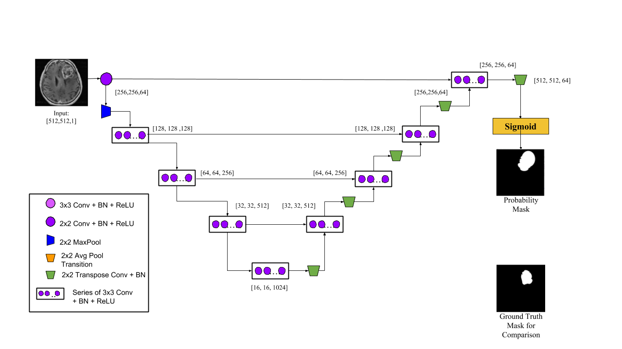
Figure 2: The baseline UNet model.

Organ	Modality	Model: UNet
Brain	MR	0.5231
Lung	CT	0.6646

Table 1: Dice score for the baseline UNet model on the brain and lung datasets.

1 Implementation

A basic UNet architecture was implemented to provide a baseline performance benchmark on the Stanford dataset. The encoder portion was implemented by incrementally increasing the number of feature maps by powers of two, from 64 filters to 1024 filters at the bottom of the “U”, at the lowest resolution, to capture intricate details regarding the lesion shapes. In the decoder portion, we symmetrically decrease the number of feature maps by powers of 2, from 1024 to 64. The final image is passed through a sigmoid layer to produce the final binary segmentation map.

Convolution:

Each convolutional layer in the proposed architecture consists of a learned kernel $W$, a batch normalization, and a ReLU unit $r(X)=\max(0,X)$; that is:

$$c(X,W,\gamma)=r(b((X*W)),\gamma),$$ (1)

where batch normalization $b(X,\gamma)$ transforms the mean of each channel to 0 and the variance to a learned per-channel scale parameter $\gamma$. The ReLU unit introduces non-linearity and assists in gradient propagation. Each convolutional block consists of a series of $c(X,W,\gamma)$ layers, as demonstrated in Figure 2.

2 Results and Analysis

Table 1 shows the results of the UNet model. It is clear that the UNet architecture alone is not enough to perform accurate segmentation. This could be due to the fact that some lesions are so small that as the encoder reduces resolution, shape information is lost, which hinders the ability of the model to pick up detailed lesion shapes. Therefore, we will improve the model by replacing the basic convolutional blocks of the UNet with dense blocks.

2 Dense UNet

In the next iteration of the model, the convolutional blocks are replaced with dense blocks, as described by Huang et al. (2016). The advantage of utilizing dense blocks is that each dense block is fed information from all previous layers, as was discussed in Section 2.3.2. Therefore, information learned from shallower layers is not lost by the deeper layers. Dense blocks consist of bottleneck layers. To move from one dense block to the next in the network, transition layers are utilized. The implementation of the bottleneck and transition layers are described in more detail in the next section.

1 Implementation

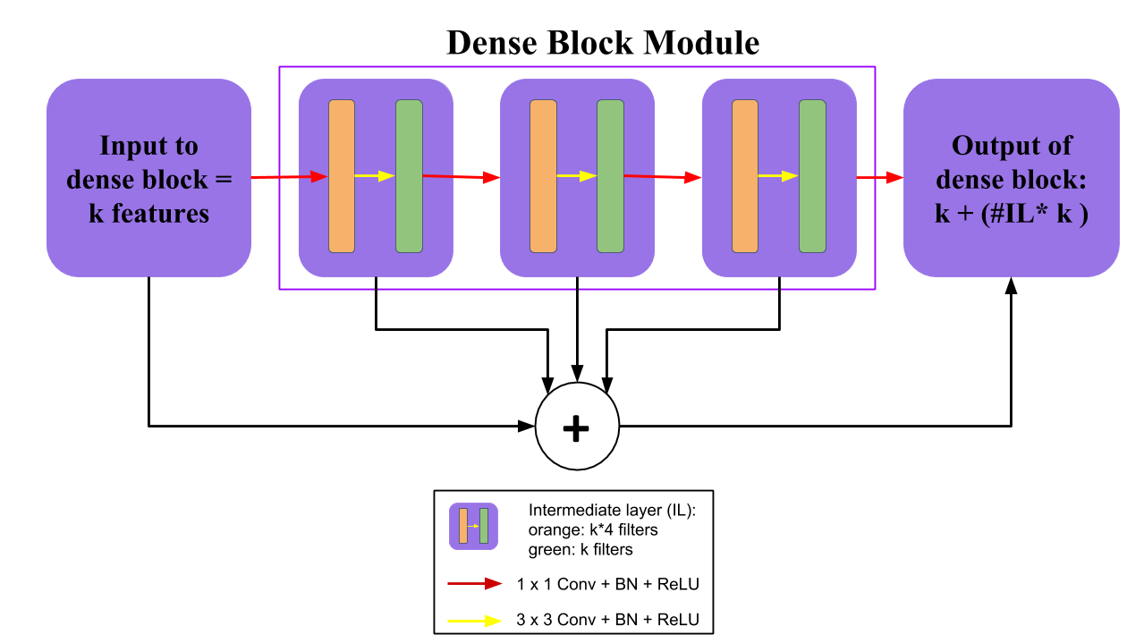
Figure 3: Dense block module. $k$ is the growth rate. Before every dense block there are $k$ feature maps generated by the transition layer. Within the dense block, there are $n$ intermediate layers (IL), each contributing $k$ feature maps (green block). The total number of feature maps produced is $k+(n\times k)$ or, the sum of the input maps and $k$ times the number of intermediate layers.

Dense Blocks:

The classic convolution blocks in UNets are replaced with a version of dense blocks. Figure 3 illustrates the implementation of the dense block module. Dense blocks take in all features learned from previous layers and feed it into subsequent layers via concatenation. Dense connectivity can be formulated as follows:

$$X_{l}=H_{l}([x_{l0},x_{l1},...,x_{l-1}]),$$ (2)

where $H()$ can be considered a composite function of batch normalization, convolution, and ReLU unit, and $[x_{0},x_{1},...,x_{l−1}]$ represents the concatenation of all feature map from layers 0 to $l-1$. This is a more memory efficient because the model is not learning redundant features by duplicating feature maps. Direct connections are implemented between feature maps learned at shallow levels to deeper levels.

The number of feature maps that are generated by each dense block is dictated by a parameter called the growth rate. For any dense block $i$, the number of feature maps is calculated as

$$f_{i}=k+(k\times n),$$ (3)

where $k$ is the growth rate and $n$ is the number of dense connections to be made. Figure 3 presents a visual representation of the feature maps in a dense block. Before every dense block $k$ feature maps are generated by the transition layer. The growth rate regulates how much new information each layer contributes to the global state. Within the dense block itself, $n$ connections are made; hence, the total number of filters is the sum of the two values. It was found that for smaller datasets, smaller values of $k$ (16–20) suffice to learn nuances of the data without overfitting, but perform better than a standard UNet.

Bottleneck Layer:

The dense UNet model has a moderate number of parameters despite concatenating many residuals together, since each $3\times 3$ convolution can be augmented with a bottleneck. A layer of a dense block with a bottleneck is as follows:

1. Batch normalization;

2. $1\times 1$ convolution bottleneck producing growth rate $\times 4$ feature maps;

3. ReLU activation;

4. Batch normalization;

5. $3\times 3$ convolution producing growth rate feature maps;

6. ReLU activation.

Transition Layer:

Transition layers are the layers between dense blocks. They perform convolution and pooling operations. The transition layers consist of a batch normalization layer and a $1\times 1$ convolutional layer followed by a $2\times 2$ average pooling layer. The transition layer is required to reduce the size of the feature maps by half before moving to the next dense block. This is useful for model compactness. A transition layer is as follows:

1. Batch normalization;

2. $1\times 1$ convolution;

3. ReLU activation;

4. Average pooling.

Figure 4 illustrates the full dense UNet architecture.

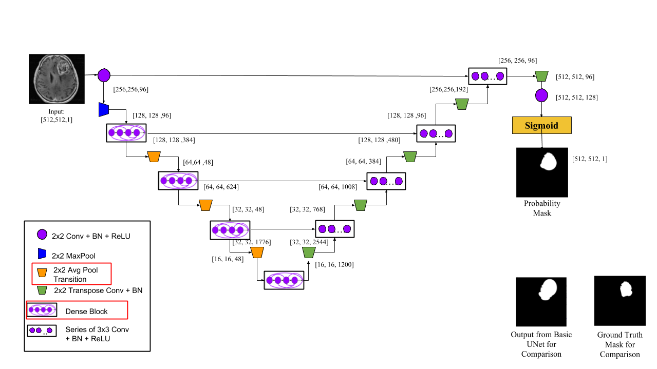
Figure 4: Dense UNet model. In this design, convolutional blocks from Figure 2 are replaced with dense block on the encoder side. Transition layers are added for model compactness. The new modifications to this model are highlighted in red in the key.

Organ	Modality	Model: Dense UNet
Brain	MR	0.5839
Lung	CT	0.6723

Table 2: Dice score for the dense UNet model on the brain and lung datasets.

2 Results and Analysis

Table 2 shows the results of the dense UNet model. There are many advantages of using the dense block modules. Recent work shows that with deeper convolutional networks, prediction accuracy is increased by creating shorter connections to layers close to both the input and the output, so that information is not lost as the network reaches deeper layers. In the standard UNet, let us assume each convolutional block has $L$ layers. This means there are only $L$ connections (one between each layer; i.e., the output of one layer is the input of next, and the next layer does not have information about layers prior to its immediate neighbor). In the case of dense blocks, $L\times(L+1)/2$ direct connections are being fed into the next block (i.e., direct, shorter connections to the input and output). This is advantageous for several reasons. Because of these direct connections, the vanishing gradient problem is alleviated, and there is stronger feature propagation so that deeper layers do not lose information learned early on in the network as the resolution decreases. This also helps with memory. With careful concatenation, deeper layers have access to feature maps of shallow layers with only one copy of these feature maps in memory, instead of multiple copies.

3 Dilated Dense UNet

Next, we implement a 2D dilated dense UNet for predicting a binary segmentation of a medical image. This architecture is described in Figure 5. First, the traditional convolution blocks of a UNet are replaced with dense blocks. Second, an up-convolution method with learnable parameters is utilized. Third, dilation is added at the bottom of the architecture for better spatial understanding.

As can be seen in Figure 5, the structure remains similar to that of the UNet; however, there are key differences that enable this model to outperform the basic UNet for the medical image segmentation task. Unlike feed-forward convolutional neural networks, in which each layer only receives the feature maps from the previous layer, for maximal information gain per convolution, every layer of the dilated dense UNet structure takes as input all the feature maps learned from all the previous layers via dense blocks. This results in a model that has an overall greater understanding from a dataset providing a limited number of examples from which to learn and generalize. In the dense blocks, to prevent redundant learning, each layer takes what has been previously learned as input. To increase spatial understanding, dilation is added to the convolutions to further increase receptive fields at reduced resolutions and understand where lesions are relative to other lesions during segmentation. The decoder portion employs a series of up-convolution and concatenation with extracted high-resolution features from the encoder in order to gain better localization. The dilated dense UNet was designed to allow lower level features to be extracted from 2D input images and passed to higher levels via dense connectivity to achieve more robust image segmentation.

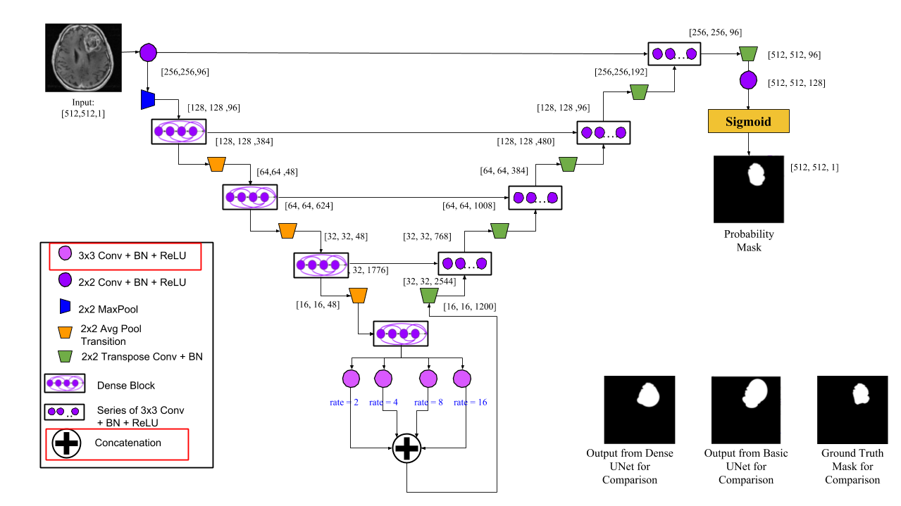
Figure 5: Dilated Dense UNet model. In this design, dilation is added to the bottom of the network. The new modifications to this model are highlighted in red in the key.

Organ	Modality	Model: Dilated Dense UNet
Brain	MR	0.6093
Lung	CT	0.6978

Table 3: Dice score for the dilated dense UNet model on the brain and lung datasets.

1 Implementation

Upconvolution:

As opposed to the bilinear interpolation proposed by Ronneberger et al. (2015), we propose a different method of upsampling on the decoder side—Transpose convolutions are used to upsample. The reason is that this method has parameters that can be learned while training, as opposed to a fixed method of interpolating. This allows for an optimal upsampling policy.

Dilation:

Dilated convolutions utilize sparse convolution kernels with large receptive fields, spatial understanding, and the advantage of few training parameters. Dilation is added to the bottom of the architecture, as shown in Figure 5.

The last dense block at the end of the contracting path is fed into 4 convolutional layers with dilation 2, 4, 8, and 16. Once the blocks go through the dilated convolutions, they are concatenated to gain wider spatial perspective at the end of the contracting path of the dilated dense UNet. This is only effective and necessary at the end of the contracting path because this area samples at the lowest resolution and can lose track of spatial understanding. Therefore expanding the spatial context with dilation before continuing on the expanding path is an efficient and effective method to obtain better results.

2 Results and Analysis

Table 3 shows the results of the dilated dense UNet model. We observed that the dilated dense UNet model performed the best compared to the baseline UNet and the Dense UNet.

The dilated dense UNet served as the backbone for a full segmentation pipeline proposed in our CVPR 2019 submission. The dilated dense UNet produces an initial segmentation map. This map is fed into two functions to generate two probability feature maps $\lambda_{1}$ and $\lambda_{2}$, which the ACL employs to produce a detailed boundary, thus achieving more accurate segmentation results.

Figure 6: Examples of final segmentation outputs. (a) Ground Truth (b) Dilated Dense UNet output (c) DLAC output

Figure 6 shows some examples of the final segmentations on the Stanford dataset produced by the dilated dense UNet and dilated dense UNet + ACL models, in comparison to the ground truth. As a backbone, the dilated dense UNet does an exceptional job of localizing and determining an initial boundary of the lesions. The ACL supports the model further to refine the boundaries. Figure 6b validates that the dense dilated UNet can also be used as an effective, automated, and accurate stand-alone architecture for lesion segmentation, as well. We also note that this same architecture was successful for two different modalities, namely MR and CT. Thus, we show that our custom dilated dense UNet is an effective backbone for the task of lesion segmentation for brain and lung.

4 Loss Function and Evaluation Metrics

As the loss function, we utilize the Dice coefficient defined in Equation 3. It performs exceptionally on problems for which there is heavy class imbalance in the training dataset. This is indeed the case for the task of lesion segmentation, as can be seen in Figure 1. In the case of brain and lung segmentation, because lesions are very small, there is a clear “class imbalance” between the number of pixels in the background and foreground of the image.

5 Effects of Using Pretrained Models

An issue with segmentation involving medical images is the lack of large aggregate datasets. The proposed models required 2D images labeled with binary masks indicating the location of lesions. The Stanford dataset is rather small to see the full potential of this model. When the model was initially trained on this small dataset, nice learning trends were not observed. The model overfit rather quickly. We hypothesized that this was because there were not enough examples to properly generalize the model. Therefore, we ran experiments with and without the use of pretrained models. The results are reported in Table 4.

Organ	UNet	DUNet	Dilated DUNet	UNet (P)	DUNet (P)	Dilated DUNet (P)
Brain	0.5231	0.5839	0.6093	0.5873	0.6105	0.7541
Lung	0.6646	0.6723	0.6978	0.7137	0.7028	0.8231

Table 4: Model evaluations. Dice values for each model are presented; (P) indicates that the model utilized pretrained weights. DUNet denotes the dense UNet.

The segmentation of lesions is a particularly difficult task because priors cannot be utilized for predicting the shapes of lesions, since each lesion is unique. The results in Table 4 indicate that using a pretrained model is clearly an effective strategy to help the model learn with such a small dataset. Pretraining can be thought of as a kind of “prior” added to the model to assist in the learning process when training on the dataset of interest. The pretraining allowed the 2D dilated dense UNet model to segment lesions with a Dice score of 82% for lung and 75% for brain images.

Chapter 4 3D Medical Image Segmentation

In recent years, the rise of deep learning models for 2D medical image segmentation has been very prevalent and successful. The same trend is starting to be observed for 3D medical data. After discussing the implementations of deep learning models for 2D medical image segmentation, this chapter transitions to exploring and validating the considerations to take into account when developing deep learning models for 3D medical image segmentation. There are many advantages to 3D medical image datasets. 3D datasets offer spatial coherence, which is quite beneficial for segmentation tasks. Although the availability of 3D data is limited, it provides important information that can help a deep model learn more accurate segmentation parameters. However, although 3D data provides rich information unavailable in 2D data, 3D data poses many challenges and transitioning to 3D is far from trivial. This chapter presents important considerations for preprocessing datasets and implementing an efficient 3D medical image segmentation model. The effectiveness of these considerations are evaluated by testing them on an abdominal lymph node dataset (Seff et al., 2015). A 3D VNet model is then trained using this dataset.

1 Background and Dataset

Lesion and organ segmentation of 3D CT scans is a challenging task because of the significant anatomical shape and size variations between different patients. Much like in the 2D case, 3D medical images suffer from low contrast from surrounding tissue, making segmentation difficult.

An interesting application for 3D medical imaging is the segmentation of CT scans of the human abdomen to detect swollen lymph nodes. Lymph nodes are small structures within the human body that work to destroy harmful substances. They contain immune cells that can help fight infection by attacking and destroying microbes that are carried in through the lymph fluid. Therefore, the lymphatic system is essential to the healthy operation of the body. The presence of enlarged lymph nodes is a signal to the onset or progression of an infection or malignancy. Therefore accurate lymph node segmentation is critical to detect life threatening diseases at an early stage and support further treatment options.

The task of detecting and segmenting swollen lymph nodes in CT scans comes with a number of challenges. One of the biggest challenges in segmenting CT scans of lymph nodes in the abdomen is that the abdominal region exhibits exceptionally poor intensity and texture contrast among neighboring lymph nodes as well as the surrounding tissues, as shown in Figure 1. Another difficulty is that low image contrast makes boundary detection between lymph nodes extremely ambiguous and challenging (Nogues et al., 2016).

Figure 1: Examples of the top (a1, a3), side (a2, a4) and front view (b2, b4) CT scans. The ground truth masks are depicted in red (b1, b3). The low contrast in the CT scans make distinguishing the lymph node from the surrounding tissue a difficult task, even for the human eye.

2 3D Data Preprocessing Techniques

There are several key points to consider when developing a 3D segmentation architecture, aside from how to fit large 3D images into memory. The first is the preprocessing techniques to be used on the dataset of interest, including image orientation and normalization methods. Another important consideration that makes a substantial difference in performance for 3D segmentation is the loss function that is utilized for training. Thus, the key considerations are as follows:

1. Consistent Orientation Across Images: Orientation is important in the 3D space. Orienting all images in the same way while training reduces training time because it does not force the model to learn all orientations for segmentation.

2. Normalization: This is a key step and there are differing techniques for different modalities.

3. Generating Segmentation Patches: This is an important strategy to use if there are memory constraints, which is often the case for 3D medical images. This strategy also aids in the issue of class imbalance in datasets.

4. Loss Functions and Evaluation Metrics: Loss functions are important considerations for 3D segmentation and can also aid in the issue of class imbalance in datasets.

To alleviate the issues listed above and properly preprocess the 3D data, the lymph node dataset was fed through the pipeline shown in Figure 2. The next sections describe the preprocessing steps in more detail.

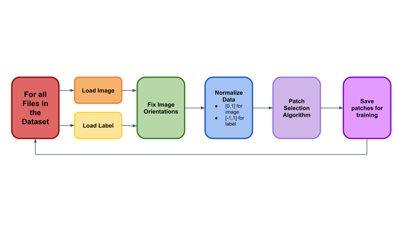
Figure 2: Preprocessing pipeline for 3D dataset.

1 Consistent Orientation

In 3D images, the idea of orientation becomes an issue of interest. Consistent orientation among all images is important to speed up training time. If there are multiple orientations, the network is forced to learn all orientations, and in order to generalize, more data is required, which is not easily available for 3D medical images. Nibable, an open source python library to read in medical images, was utilized to determine 3D image orientation and reorient images if necessary. It was found that the orientation itself did not make a difference on training so long as the orientation was consistent throughout the dataset.

2 Normalization

Normalization is a key step in the preprocessing pipeline for any deep learning task. Normalization is also very important for medical images and there are a variety of methods for doing this. The aim of normalization is to remove heavy variation in data that does not contribute to the prediction process and instead accentuate the features and differences that are of most importance. The following methods may be used specifically for medical image segmentation (Rajchl, 2018):

1. Voxel Intensity Normalization: This method is very dependent on the imaging modality. For images such as weighted brain MR images, a zero-mean unit variance normalization is the standard procedure. This is done because the contrast in the image is usually set by an expert taking the MR images and thus there is high variation in intensity across image sets. This variation may be considered noise. To standardize intensity across multiple intensity settings, we use a zero mean normalization. In contrast, CT imaging measures a physical quantity such as radio-density in CT imaging, where the intensities are comparable across different scanners. Therefore, for this modality, the standard normalization methodology is clipping or rescaling to a range such as $[0,1]$ or $[-1,1]$.

2. Spatial Normalization: Normalizing for image orientation avoids the need for the model to learn all possible orientations of input images. This reduces both the need for a large amount of training data and training time. Since, as mentioned previously, properly labeled medical data is often meagre in quantity, this is a very effective technique of normalization.

Since the the modality of the abdominal lymph node data was 3D CT scans, both methods of normalization were used. Reorientation was also done on all images. Voxel intensity normalization was performed by rescaling all voxels in the images to a range of $[-1,1]$ and the voxels in the labels to $[0,1]$.

3 Generating Segmentation Patches

Patch-based segmentation is used to tackle the issue of limited memory. A single 3D image in the lymph node dataset was $512\times 512\times 775$. With the memory constraints, using these raw images would only allow for a batch size of 1, which would result in an incredibly long training time, and very little flexibility to extend the deep learning architecture. Therefore patch-based segmentation was utilized.

The basic idea of patch generation is to take in an input image, determine the regions of greatest interest in the image, and return a smaller portion of the image, focusing on these regions of importance. Doing this is important for many reasons. The first reason is that having smaller image sizes allows for larger batch sizes and faster training. The second reason is that the data is naturally augmented with this process. The third reason is that class imbalance issues can be avoided. Class imbalance occurs when a sample image has more voxels belonging to one class over another. Figure 1 shows this very clearly. In the example, the majority of the voxels belong to the background (black) class and a small subset belong to the foreground (red) class. Feeding such images directly to the model will cause the the model to skew its learning to favor the background voxles. Therefore, intelligent selection of patches is key to training. For this work, we generated patches of $128\times 128\times 128$. We utilized the Deep Learning Toolkit to generate our class-balanced segmentation patches.

Unlike during training time, in which the patches are generated randomly around areas of interest, during test time, the images are systematically broken into $128\times 128\times 128$ chunks. Prediction is done on each chunk and the chunks are joined together for the final prediction. The patching technique alone creates some discrepancies at the boarders of patches, so smoothing is performed to obtain a more seamless prediction.

4 Loss Functions and Evaluation Metrics

The choice of loss functions can significantly affect the performance of 3D segmentation architectures. In medical images, it is very common that the region of interest, for example, a lesion, covers a very small portion of the scan. Therefore, during the learning process, the network often gets stuck in local minima due to this class imbalance of background and foreground pictures. This causes poor results during training and testing since the prediction of both classes is weighed equally. This causes the model to be biased toward the background voxels and the foreground is either completely missed or partially detected. The following losses attempt to address these issues.

Jaccard Coefficient and Loss

The Jaccard coefficient is measure of similarity between a ground truth mask and a prediction mask. Lets assume that all voxels in the ground truth mask are in set $G$. All voxels in the prediction mask are in set $P$. The Jaccard coefficient calculates the ratio of 3 mutually exclusive partitions: $|P\cap G|$, $|P\setminus G|$, $|G\setminus P|$. The equation for the Jaccard coefficient is

$$\begin{split}J=\frac{|P\cap G|}{|P\cap G|+|P\setminus G|+|G\setminus P|},\end{split}$$ (1)

and the full loss function is defined as $1-J$, where the $|P\setminus G|$ notation refers to the set of elements in $P$ but not in $G$. The Jaccard coefficient calculates the overlap ratio between a ground truth mask and a predicted mask by giving equal weightage to $|P\cap G|$, $|P\setminus G|$, $|G\setminus P|$. If the data of interest does not suffer too much from class imbalance, the Jaccard coefficient and loss is a good metric to measure the success of a model. If there is class imbalance, this method may not produce as promising results and a model could become biased towards the dominating class.

Dice Coefficient and Loss:

The Dice coefficient is a metric that compares the similarity between a ground truth mask and a prediction mask. It is similar to the Jaccard coefficient with one subtle but significant difference—in the way class imbalance is handled. Dice Loss was used in Chapter 4, as it is a common loss function for both 2D and 3D medical image segmentation. The Dice coefficient, also known as the Sorensen-Dice coefficient, is defined as

$$D=\frac{2\times|P\cap G|}{2\times|P\cap G|+|P\setminus G|+|G\setminus P|}$$ (2)

and the Dice Loss is defined as $1-D$. The Dice coefficient is a measure of similarity between two sets. The Dice coefficient addresses the issue of class imbalance by calculating the overlap between a prediction and a ground truth mask for a region of interest. The Dice coefficient is unique because unlike the Jaccard metric, the Dice metric gives more weight to voxels that belong to both sets (a.k.a. the overlapping region of both sets) when calculating the overlap ratios, hence the factor of 2 that is multiplied to the union sum in the numerator. For this reason, the Dice metric and loss function is often utilized for medical image segmentation since correct overlapping regions are hard to find due to irregular lesion shapes.

Tversky Coefficient and Loss:

The Tversky coefficient is yet another similarity metric related to both the Jaccard and Dice coefficients with a different method of handling class imbalance. The Tversky Coefficient is defined as

$$T=\frac{|P\cap G|}{|P\cap G|+\alpha|P\setminus G|+\beta|G\setminus P|}$$ (3)

and the Tversky Loss is defined as $1-T$, where $\alpha$ and $\beta$ control the magnitude of penalties of false positive versus false negative errors in the pixel classification for segmentation. The ranges of the $\alpha$ and $\beta$ hyperparameters, which can be tuned to produce optimal loss results on the dataset of interest, must be such that $\alpha+\beta=1$. The Tversky metric provides a spectrum of methods to normalize the size of a two-way set intersection. The Tversky index can be thought of as a generalized Dice index, since the Dice coefficient is the Tversky coefficient with $\alpha=\beta=0.5$.

3 3D VNet Implementation and Data Processing Pipeline

Our base implementation of the VNet architecture was inspired by the work of Ko (2018). The main portions of this architecture involved a data-loader, the VNet model, and an evaluation pipeline to see how well the model can predict on new images. However, the pipeline had to be heavily modified. In medical imaging, data input-output is often one of the most challenging steps. This is especially challenging for the case of 3D images, since special care must be taken to load and preprocess the data. The initial data-loader and training pipeline involved using the SimpleITK package to read in, normalize, and randomly select patches on which to train the model. The disadvantage to using SimpleITK is that this library does not utilize GPU-accelerated operations, making the data-loader slow and inefficient. SimpleITK was also utilized for the evaluation pipeline. Since SimpleITK is not GPU-compatible, memory constraints were an initial problem. Therefore, the data-loader and evaluation pipelines were then changed to utilize the Nibabel and Deep Learning Toolkit (DLTK) packages. The Nibabel package was used to read in a image, normalize the image, and orient all images in the same way. The DLTK package was used to select patches on which to train the model. DLTK utilizes an algorithm that determines the regions of interest in each image and creates patches around this region to promote class-balanced samples. This improved end-to-end pipeline was utilized to train the VNet model to predict swollen lymph nodes in 3D abdominal CT scans.

1 Results and Analysis

Figure 3: (a)Examples of segmentation overlaid with ground truth masks. (b) Examples of segmentation overlaid with predicted masks. In each set of 4 images, the top left is a top view, top right is a side view, bottom left is the segmentation mask, bottom right is a front view. (1) shows results from a few hours of training. (2) show results from a few days of training.

Figure 3 shows our preliminary results of this model on the lymph node dataset. The 3D VNet model was trained using a Dice loss function. Figure 3a depicts the CT scans overlaid with the ground truth masks. Within each group of four images, the lower left depicts the 3D isolated lymph nodes. Figure 3b depicts the CT scans overlaid with the predicted masks from this VNet architecture. Again, in the groups of four, the lower left image shows the isolated 3D mask prediction. For Figure 3a, it is evident how difficult this problem is, due to small size of the lymph nodes compared to the rest of the body. These preliminary results were obtained by training 1. for few hours (Figure 3 (1)) and 2. for a few days (Figure 3 (2)). An interesting observation is that even within a few hours, the VNet started to distinguish boundaries in the image, which explains why the bottom left image in Figure 3 (b1) look like the outline of the patient in 3D. After training the model for a few days, it was observed that even more details are learned by the VNet, such as the ribs (Figure 3 (b2)). This trend suggests that if the model was trained long enough, or was trained using more computational resources, it would start to pick up the nuances of the lymph nodes. However, this also suggests that there are many improvements that could be made to this model to enable better performance, such as adding dense connectivity to the VNet, similar to the 2D version in Chapter 4, different loss functions, or different styles of encoder-decoder architectures. Due to time constraints, we were unable to be perform exhaustive evaluation metrics and trials on the effects of different loss functions for this dataset. However, this work has set the foundation for many future endeavors and extensions of our work.

Chapter 5 Conclusion

Image segmentation is a topic of great interest in computer vision and it has been utilized for a variety of tasks, such as object localization and recognition, boundary detection, autonomous driving, and medical imaging. Prior successful segmentation methods relied on some level of manual user initialization. This thesis proposed effective architectures to fully automate the process of localizing and delineating boundaries of objects in images. In particular, we developed and implemented deep learning frameworks for two segmentation tasks, namely salient object detection and 2D medical image segmentation. We also explored and evaluated the considerations that should be taken into account when moving from 2D medical image segmentation to 3D, thereby setting the foundation for future extensions of our 2D models to 3D.

First, we addressed the problem of salient object detection. Several encoder-decoder architectures were described before arriving at a novel dilated dense encoder-decoder network with dilated spatial pyramid pooling. Serving as the backbone CNN architecture in conjunction with an active contour layer, our full pipeline outperformed on one of the three popular datasets used for salient object detection, and was very competitive on the other two datasets. The segmentation results of the dilated dense encoder-decoder itself were also impressive, indicating that this architecture can serve as a robust stand-alone segmentation architecture as well.

Next, we addressed an important and relevant use case of segmentation, namely 2D medical image segmentation. We developed a novel dilated dense UNet architecture to combat the many challenges faced with 2D lesion segmentation, including low image contrast, lack of large labeled datasets, and the lack of robust pretrained models. A custom dataset from a collaboration with Stanford University was utilized to evaluate our model’s performance. Compared to the baseline, our dilated dense UNet model demonstrated significantly better performance, confirming the effectiveness of our architecture. Our architecture was used as the backbone CNN for accurate initial lesion localization and boundary delineation in a full pipeline, which also combined active contours. The segmentation results of the stand-alone dilated dense UNet also showed promising results for 2D lesion segmentation, suggesting that it can perform well on its own.

1 Future Work

Our discussion in Chapter 5 set the foundation for developing a robust 3D model for medical image segmentation, which is important since modern medical imaging systems often acquire 3D images. There are many possible improvements to our model, including exploring additions to the basic VNet architecture, how different loss functions affect training, or experimenting with the effectiveness of using greater computational resources, if available.

1 Additional Loss Functions

For the VNet model, a Dice loss function was utilized. This was chosen because it is the most popular metric for the case of medical image segmentation. However, one should experiment with other loss functions to determine which is most effective at handling class imbalance in datasets. For the case of lymph node segmentation, there was heavy class-imbalance, as observed in Figure 3a. Therefore, a useful loss function to explore could be the Tversky loss function. Weighted Cross Entropy is yet another effective loss function utilized in more general segmentation tasks. Multi-layered loss functions are another interesting option to explore.

2 Additions to the VNet Architecture

The first suggested modification, in conjunction to the previous chapters of this work, is to experiment with adding dense blocks to the VNet architecture. As seen in the 2D case, it is reasonable to hypothesize that adding dense connectivity will increase the learning capabilities of the model because each layer will directly take as input all previously learned feature maps. For challenging segmentation tasks, such as swollen lymph node segmentation, we observed that the learning process is rather slow. Dense connectivity could also help speed up the learning process due to the easier flow of gradients during backpropagation. Another suggested modification to the VNet architecture is to add dilated convolutions to gain spatial awareness on the encoder side of the VNet. Dilated convolutions can be useful in the 3D case because they are computationally efficient with the advantage of an expanded receptive field, which is critical in the 3D case.

3 Additional Computational Resources

All the work presented in this thesis utilized a single Nvidia 1080 Ti GPU. This was a powerful resource effectively training the 2D models developed in Chapters 3 and 4 on $256\times 256$ and $512\times 512$ images. For the 3D datasets, the image sizes varied from $512\times 512\times 48$ to $512\times 512\times 775$. These images were much too large to fit more than one into memory at a time. Therefore, a patch based method was adopted to train the segmentation model. Although our preliminary results suggested the potential effectiveness of the patch based approach to training, given greater resources permitting the accommodation of an entire image for training, it seems reasonable to expect that even a basic VNet model would be much more effective and robust. Regardless of the computational resource limitation, however, our work demonstrates a series of highly effective 2D models and sets the stage for extending them to the purposes of 3D medical image analysis.

In the recent past, a number of tasks dependent on image segmentation have come to light, such as medical imaging, autonomous driving, or scene understanding. This research work hoped to gain a deeper understanding of image segmentation and contribute to this topic, which has become critical to understanding and assisting the world around us.

References

- Aggarwal et al. (2011) Aggarwal, P., Vig, R., Bhadoria, S., and Dethe, C. (2011). Role of segmentation in medical imaging: A comparative study. International Journal of Computer Applications (0975 8887), 29(1).
- Badrinarayanan et al. (2015) Badrinarayanan, V., Kendall, A., and Cipolla, R. (2015). Segnet: A deep convolutional encoder-decoder architecture for image segmentation. arXiv preprint arXiv:1511.00561.
- Bogue (2005) Bogue, R. (2005). Machine vision theory, algorithms, practicalities. Assembly Automation, 25(3).
- Boykov and Jolly (2001) Boykov, Y. Y. and Jolly, M.-P. (2001). Interactive graph cuts for optimal boundary and region segmentation of objects in ND images. In Computer Vision, 2001. ICCV 2001. Proceedings. Eighth IEEE International Conference on, volume 1, pages 105–112. IEEE.
- Deng et al. (2009) Deng, J., Dong, W., Socher, R., Li, L.-J., Li, K., and Fei-Fei, L. (2009). Imagenet: A large-scale hierarchical image database. In 2009 IEEE conference on computer vision and pattern recognition, pages 248–255. Ieee.
- Gibson et al. (2018) Gibson, E., Giganti, F., Hu, Y., Bonmati, E., Bandula, S., Gurusamy, K., Davidson, B., Pereira, S. P., Clarkson, M. J., and Barratt, D. C. (2018). Automatic multi-organ segmentation on abdominal CT with dense V-networks. IEEE Transactions on Medical Imaging, 37(8):1822–1834.
- Han et al. (2015) Han, J., Zhang, D., Hu, X., Guo, L., Ren, J., and Wu, F. (2015). Background prior-based salient object detection via deep reconstruction residual. IEEE Transactions on Circuits and Systems for Video Technology, 25(8):1309–1321.
- Hatamizadeh et al. (2018) Hatamizadeh, A., Ananth, S. P., Ding, X., Terzopoulos, D., Tajbakhsh, N., et al. (2018). Automatic segmentation of pulmonary lobes using a progressive dense v-network. In Deep Learning in Medical Image Analysis and Multimodal Learning for Clinical Decision Support, pages 282–290. Springer.
- Hatamizadeh et al. (2019a) Hatamizadeh, A., Hoogi, A., Lu, W., Sengupta, D., Wilcox, B., Rubin, D., and Terzopoulos, D. (2019a). Deep level-set active contour models for lesion segmentation. arXiv preprint.
- Hatamizadeh et al. (2019b) Hatamizadeh, A., Hoogi, A., Sengupta, D., Lu, W., Wilcox, B., Rubin, D., and Terzopoulos, D. (2019b). Deep active lesion segmentation. arXiv preprint arXiv:1908.06933.
- Hatamizadeh et al. (2019c) Hatamizadeh, A., Hosseini, H., Liu, Z., Schwartz, S. D., and Terzopoulos, D. (2019c). Deep dilated convolutional nets for the automatic segmentation of retinal vessels. arXiv preprint arXiv:1905.12120.
- Hatamizadeh et al. (2019d) Hatamizadeh, A., Sengupta, D., and Terzopoulos, D. (2019d). End-to-end deep convolutional active contours for image segmentation. arXiv preprint.
- Hatamizadeh et al. (2019e) Hatamizadeh, A., Terzopoulos, D., and Myronenko, A. (2019e). End-to-end boundary aware networks for medical image segmentation. arXiv preprint arXiv:1908.08071.
- He et al. (2016) He, K., Zhang, X., Ren, S., and Sun, J. (2016). Deep residual learning for image recognition. In Proceedings of the IEEE Conference on Computer Vision and Pattern Recognition, pages 770–778.
- Hinton et al. (2012) Hinton, G. E., Krizhevsky, A., and Sutskever, I. (2012). Imagenet classification with deep convolutional neural networks. Advances in neural information processing systems, 25:1106–1114.
- Hou et al. (2017) Hou, Q., Cheng, M.-M., Hu, X., Borji, A., Tu, Z., and Torr, P. (2017). Deeply supervised salient object detection with short connections. In Proceedings of the IEEE Conference on Computer Vision and Pattern Recognition.
- Huang et al. (2016) Huang, G., Liu, Z., and Weinberger, K. Q. (2016). Densely connected convolutional networks. CoRR, abs/1608.06993.
- Kass et al. (1988) Kass, M., Witkin, A., and Terzopoulos, D. (1988). Snakes: Active contour models. International Journal of Computer Vision, 1(4):321–331.
- Ko (2018) Ko, J. K. (2018). Implementation of Vnet in TensorFlow for medical image segmentation. https://github.com/jackyko1991/vnet-tensorflow.
- Korn et al. (1996) Korn, F., Sidiropoulos, N., Faloutsos, C., Siegel, E., and Protopapas, Z. (1996). Fast nearest neighbor search in medical image databases. In Proceedings of the 22nd VLDB Conference, pages 215–226.
- Krizhevsky et al. (2012) Krizhevsky, A., Sutskever, I., and Hinton, G. E. (2012). Imagenet classification with deep convolutional neural networks. In Advances in Neural Information Processing Systems, pages 1097–1105.
- Kurtulmus (2017) Kurtulmus, B. (2017). Introduction to image saliency detection. https://blog.algorithmia.com/introduction-image-saliency-detection/.
- Lee et al. (2016) Lee, G., Tai, Y.-W., and Kim, J. (2016). Deep saliency with encoded low level distance map and high level features. In Proceedings of the IEEE Conference on Computer Vision and Pattern Recognition, pages 660–668.
- Leung and Malik (1998) Leung, T. and Malik, J. (1998). Contour continuity in region based image segmentation. In European Conference on Computer Vision, pages 544–559. Springer.
- Li et al. (2011) Li, C., Huang, R., Ding, Z., Gatenby, J. C., Metaxas, D. N., and Gore, J. C. (2011). A level set method for image segmentation in the presence of intensity inhomogeneities with application to MRI. IEEE Transactions on Image Processing, 20(7):2007–2016.
- Li and Yu (2015) Li, G. and Yu, Y. (2015). Visual saliency based on multiscale deep features. CoRR, abs/1503.08663.
- Li and Yu (2016) Li, G. and Yu, Y. (2016). Deep contrast learning for salient object detection. CoRR, abs/1603.01976.
- Long et al. (2015) Long, J., Shelhamer, E., and Darrell, T. (2015). Fully convolutional networks for semantic segmentation. In Proceedings of the IEEE Conference on Computer Vision and Pattern Recognition, pages 3431–3440.
- Ma et al. (2009) Ma, Z., Tavares, J., Natal Jorge, R., and Mascarenhas, T. (2009). A review of algorithms for medical image segmentation and their applications to the female pelvic cavity. Computer Methods in Biomechanics and Biomedical Engineering, 13:235–46.
- Milletari et al. (2016) Milletari, F., Navab, N., and Ahmadi, S.-A. (2016). V-Net: Fully convolutional neural networks for volumetric medical image segmentation. In Fourth International Conference on 3D Vision (3DV), pages 565–571. IEEE.
- Mishra et al. (2011) Mishra, A. K., Fieguth, P. W., and Clausi, D. A. (2011). Decoupled active contour (DAC) for boundary detection. IEEE Transactions on Pattern Analysis and Machine Intelligence, 33(2):310–324.
- Myronenko and Hatamizadeh (2019) Myronenko, A. and Hatamizadeh, A. (2019). 3d kidneys and kidney tumor semantic segmentation using boundary-aware networks. arXiv preprint arXiv:1909.06684.
- Nogues et al. (2016) Nogues, I., Lu, L., Wang, X., Roth, H., Bertasius, G., Lay, N., Shi, J., Tsehay, Y., and Summers, R. M. (2016). Automatic lymph node cluster segmentation using holistically-nested neural networks and structured optimization in CT images. In International Conference on Medical Image Computing and Computer-Assisted Intervention, pages 388–397. Springer.
- Norouzi et al. (2014) Norouzi, A., Rahim, M. S. M., Altameem, A., Saba, T., Rad, A. E., Rehman, A., and Uddin, M. (2014). Medical image segmentation methods, algorithms, and applications. IETE Technical Review, 31(3):199–213.
- Osher and Fedkiw (2001) Osher, S. and Fedkiw, R. P. (2001). Level set methods: An overview and some recent results. Journal of Computational physics, 169(2):463–502.
- Qu and Zhang (2010) Qu, Z. and Zhang, L. (2010). Research on image segmentation based on the improved Otsu algorithm. In Intelligent Human-Machine Systems and Cybernetics (IHMSC), 2010 2nd International Conference on, volume 2, pages 228–231. IEEE.
- Rajchl (2018) Rajchl, M. (2018). An introduction to biomedical image analysis with TensorFlow and DLTK. https://medium.com/tensorflow/an-introduction-to-biomedical-image-analysis-with-tensorflow-and-dltk-2c25304e7c13.
- Ronneberger et al. (2015) Ronneberger, O., Fischer, P., and Brox, T. (2015). U-net: Convolutional networks for biomedical image segmentation. In International Conference on Medical Image Computing and Computer-Assisted Intervention, pages 234–241. Springer.
- Seff et al. (2015) Seff, A., Lu, L., Barbu, A., Roth, H., Shin, H.-C., and Summers, R. M. (2015). Leveraging mid-level semantic boundary cues for automated lymph node detection. In International Conference on Medical Image Computing and Computer-Assisted Intervention, pages 53–61. Springer. https://wiki.cancerimagingarchive.net/display/Public/CT+Lymph+Nodes.
- Sermanet et al. (2013) Sermanet, P., Eigen, D., Zhang, X., Mathieu, M., Fergus, R., and LeCun, Y. (2013). Overfeat: Integrated recognition, localization and detection using convolutional networks. arXiv preprint arXiv:1312.6229.
- Simonyan and Zisserman (2014) Simonyan, K. and Zisserman, A. (2014). Very deep convolutional networks for large-scale image recognition. arXiv preprint arXiv:1409.1556.
- Szegedy et al. (2015) Szegedy, C., Liu, W., Jia, Y., Sermanet, P., Reed, S., Anguelov, D., Erhan, D., Vanhoucke, V., and Rabinovich, A. (2015). Going deeper with convolutions. In Proceedings of the IEEE conference on computer vision and pattern recognition, pages 1–9.
- Vese and Chan (2002) Vese, L. A. and Chan, T. F. (2002). A multiphase level set framework for image segmentation using the mumford and shah model. International Journal of Computer Vision, 50(3):271–293.
- Wang et al. (2017) Wang, J., Jiang, H., Yuan, Z., Cheng, M.-M., Hu, X., and Zheng, N. (2017). Salient object detection: A discriminative regional feature integration approach. International Journal of Computer Vision, 123(2):251–268.
- Yan et al. (2013) Yan, Q., Xu, L., Shi, J., and Jia, J. (2013). Hierarchical saliency detection. In Proceedings of the IEEE Conference on Computer Vision and Pattern Recognition, pages 1155–1162.
- Yu and Koltun (2015) Yu, F. and Koltun, V. (2015). Multi-scale context aggregation by dilated convolutions. arXiv preprint arXiv:1511.07122.
- Zhao et al. (2015) Zhao, R., Ouyang, W., Li, H., and Wang, X. (2015). Saliency detection by multi-context deep learning. In Proceedings of the IEEE Conference on Computer Vision and Pattern Recognition, pages 1265–1274.
- Zhu and Yuille (1996) Zhu, S. C. and Yuille, A. (1996). Region competition: Unifying snakes, region growing, and Bayes/MDL for multiband image segmentation. IEEE Transactions on Pattern Analysis and Machine Intelligence, 9:884–900.