Compressed Gradient Methods with Hessian-Aided Error Compensation

Abstract

The emergence of big data has caused a dramatic shift in the operating regime for optimization algorithms. The performance bottleneck, which used to be computations, is now often communications. Several gradient compression techniques have been proposed to reduce the communication load at the price of a loss in solution accuracy. Recently, it has been shown how compression errors can be compensated for in the optimization algorithm to improve the solution accuracy. Even though convergence guarantees for error-compensated algorithms have been established, there is very limited theoretical support for quantifying the observed improvements in solution accuracy. In this paper, we show that Hessian-aided error compensation, unlike other existing schemes, avoids accumulation of compression errors on quadratic problems. We also present strong convergence guarantees of Hessian-based error compensation for stochastic gradient descent. Our numerical experiments highlight the benefits of Hessian-based error compensation, and demonstrate that similar convergence improvements are attained when only a diagonal Hessian approximation is used.

I Introduction

Large-scale and data-intensive problems in machine learning, signal processing, and control are typically solved by parallel/distributed optimization algorithms. These algorithms achieve high performance by splitting the computation load between multiple nodes that cooperatively determine the optimal solution. In the process, much of the algorithm complexity is shifted from the computation to the coordination. This means that the communication can easily become the main bottleneck of the algorithms, making it expensive to exchange full precision information especially when the decision vectors are large and dense. For example, in training state-of-the-art deep neural network models with millions of parameters such as AlexNet, ResNet and LSTM communication can account for up to $80\%$ of overall training time, [2, 3, 4].

To reduce the communication overhead in large-scale optimization much recent literature has focused on algorithms that compress the communicated information. Some successful examples of such compression strategies are sparsification, where some elements of information are set to be zero [5, 6] and quantization, where information is reduced to a low-precision representation [2, 7]. Algorithms that compress information in this manner have been extensively analyzed for both centralized and decentralized architectures, [2, 6, 7, 8, 9, 10, 11, 12, 13, 14]. These algorithms are theoretically shown to converge to approximate optimal solutions with an accuracy that is limited by the compression precision. Even though compression schemes reduce the number of communicated bits in practice, they often lead to significant performance degradation in terms of both solution accuracy and convergence times, [4, 9, 15, 16].

To mitigate these negative effects of information compression on optimization algorithms, serveral error compensation strategies have been proposed [4, 17, 18, 16]. In essence, error compensation corrects for the accumulation of many consecutive compression errors by keeping a memory of previous errors. Even though very coarse compressors are used, optimization algorithms using error compensation often display the same practical performance as as algorithms using full-precision information, [4, 17]. Motivated by these encouraging experimental observations, several works have studied different optimization algorithms with error compensation, [18, 1, 16, 19, 15, 20, 21]. However, there are not many theoretical studies which validate why error compensation exhibits better convergence guarantees than direct compression. For instance, Wu et. al [16] derived better worst-case bound guarantees of error compensation as the iteration goes on for quadratic optimization. Karimireddy et. al [15] showed that binary compression may cause optimization algorithms to diverge, already for one-dimensional problems, but that this can be remedied by error compensation. However, we show in this paper (see Remark 1) that these methods still accumulate errors, even for quadratic problems.

The goal of this paper is develop a better theoretical understanding of error-compensation in compressed gradient methods. Our key results quantify the accuracy gains of error-compensation and prove that Hessian-aided error compensation removes all accumulated errors on strongly convex quadratic problems. The improvements in solution accuracy are particularly dramatic on ill-conditioned problems. We also provide strong theoretical guarantees of error compensation in stochastic gradient descent methods distributed across multiple computing nodes. Numerical experiments confirm the superior performance of Hessian-aided error compensation over existing schemes. In addition, the experiments indicate that error compensation with a diagonal Hessian approximation achieves similar performance improvements as using the full Hessian.

Notation and definitions. We let $\mathbb{N}$ ,$\mathbb{N}_{0}$, $\mathbb{Z}$, and $\mathbb{R}$ be the set of natural numbers, the set of natural numbers including zero, the set of integers, and the set of real numbers, respectively. The set $\{0,1,\ldots,T\}$ is denoted by $[0,T].$ For $x\in\mathbb{R}^{d}$, $\|x\|$ and $\|x\|_{1}$ are the $\ell_{2}$ norm and the $\ell_{1}$ norm, respectively, and $\left\lceil x\right\rceil_{+}=\max\{0,x\}$. For a symmetric matrix $A\in R^{d\times d}$, we let $\lambda_{1}(A),\ldots,\lambda_{d}(A)$ denote the eigenvalues of $A$ in an increasing order (including multiplicities), and its spectral norm is defined by $\|A\|=\max_{i}|\lambda_{i}(A)|$. A continuously differentiable function $f:\mathbb{R}^{d}\rightarrow\mathbb{R}$, is $\mu$-strongly convex if there exists a positive constant $\mu$ such that

$$f(y)\geq f(x)+\langle\nabla f(x),y-x\rangle+\frac{\mu}{2}\|y-x\|^{2},\quad\forall x,y.$$ (1)

and $L$-smooth if

$$||\nabla f(y)-\nabla f(x)||\leq L||x-y||,\quad\forall x,y\in\mathbb{R}^{d}.$$ (2)

II Motivation and Preliminary Results

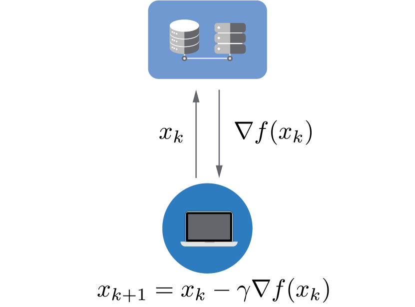
(a)

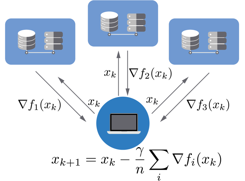
(b)

Figure 1: Two common communication architectures for distributed gradient methods: 1) full gradient communication (left) and 2) partial gradient communication (right).

In this section, we motivate our study of error-compensated gradient methods. We give an overview of distributed optimization algorithms based on communicating gradient information in § II-A and describe a general form of gradient compressors, covering most existing ones, in § II-B. Later in § III we illustrate the limits of directly compressing the gradient, motivating the need for the error-compensated gradient methods studied in this paper.

II-A Distributed Optimization

Distributed optimization has enabled solutions to large problems in many application areas, e.g., smart grids, wireless networks, and statistical learning. Many distributed algorithms build on gradient methods and can be categorized based on whether they use a) full gradient communication or b) partial gradient communication; see Figure 1. The full gradient algorithms solve problems on the form

$$\mathop{\text{missing}}{minimize}\limits_{x}\quad f(x),$$ (3)

by the standard gradient descent iterations

$$x^{k+1}=x^{k}-\gamma\nabla f(x^{k}),$$ (4)

communicating the full gradient $\nabla f(x^{k})$ in every iteration. Such a communication pattern usually appears in dual decomposition methods where $f(\cdot)$ is a dual function associated with some large-scale primal problems; we illustrate this in subsection II-A1. The partial gradient algorithms are used to solve separable optimization problems on the form

$$\mathop{\text{missing}}{minimize}\limits_{x}\quad f(x)=\frac{1}{n}\sum_{i=1}^{n}f_{i}(x),$$ (5)

by gradient descent

$$x^{k+1}=x^{k}-\frac{\gamma}{n}\sum_{i=1}^{n}\nabla f_{i}(x^{k}),$$ (6)

and distributing the gradient evaluation on $n$ nodes, each responsible for evaluating one of the partial gradients $\nabla f_{i}(x)$; see § II-A2). Clearly, full gradient communication is a special case of partial gradient communication with $n=1$. However, considering the full gradient communication algorithms separately will enable us to get stronger results for this scenario. We now review these algorithms separately in more detail.

II-A1 Full Gradient Communication (Dual Decomposition)

Resource allocation is a class of distributed optimization problems where a group of $n$ nodes aim to minimize the sum of their local utility functions under a set of shared resource constraints. In particular, the nodes collaboratively solve

$$\underset{q_{1},\ldots,q_{n}}{\text{maximize}} \sum_{i=1}^{n}U_{i}(q_{i})$$ (7)

subject to $$q_{i}\in\mathcal{Q}_{i},\leavevmode\nobreak\ \leavevmode\nobreak\ i=1,\ldots,n$$

$$h(q_{1},q_{2},\ldots,q_{n})=0.$$

Each node has a utility function $U_{i}(q)$ depending on its own private resource allocation $q_{i}$, constrained by the set ${\mathcal{Q}}_{i}$. The decision variables are coupled through the total resource constraint $h(q_{1},q_{2},\ldots,q_{n})=0$, which captures system-wide physical or economical limitations. Distributed algorithms for these problems are often based on solving a dual problem on the form (3). Here $x$ is the dual variable (associated to the coupling constraints) which is updated using the dual gradient method (4) with $f(x):=\min_{q}L(q,x)$ and

$$L(q,x)=\sum_{i=1}^{n}U_{i}(q_{i})+x^{T}h(q_{1},\ldots,q_{n}),$$

is the Lagrangian function. The dual function is convex and the dual gradient (or a dual subgradient) is given by

$$\nabla f(x)=h(q_{1}(x),\ldots,q_{n}(x)),\leavevmode\nobreak\ \leavevmode\nobreak\ \leavevmode\nobreak\ \leavevmode\nobreak\ q(x)=\underset{q}{\text{argmin}}\,L(q,x).$$

The dual gradient can often be measured from the effect of the current decisions  [22, 23, 24, 25, 7, 26]. Therefore, we get a distributed algorithm

$$q_{i}^{k+1}= \underset{q}{\text{argmin}}\leavevmode\nobreak\ U_{i}(q_{i}^{k})+(x^{k})^{T}h_{i}(q_{i}^{k}),\leavevmode\nobreak\ \leavevmode\nobreak\ \leavevmode\nobreak\ \leavevmode\nobreak\ i=1,\ldots,n$$

$$x^{k+1}= x^{k}+\gamma\nabla f(x^{k})$$

where the main communication is the transmission of the dual gradient to the users. To communicate the gradient it must first be compressed into the finite number of bits. Our results demonstrate naive gradient compression can be improved by an error correction step, leading to accuracy improvements.

II-A2 Partial Gradient Communication

Problems on the form of (5) appear, e.g., in machine learning and signal processing. One important example is empirical risk minimization (ERM) where labelled data is split among $n$ nodes which collaborate to find the optimal estimate. In particular, if each node $i\in[1,n]$ has access to its local data with feature vectors ${\bf{z}}_{i}=(z_{i}^{1},\ldots,z_{i}^{m})$ and labels ${\bf{y}}_{i}=(y_{i}^{1},\ldots,y_{i}^{m})$ with $z_{i}^{j}\in\mathbb{R}^{d}$ and $y_{i}^{j}\in\mathbb{R}$, then the local objective functions are defined as

$$f_{i}(x){=}\frac{1}{m}\sum_{j=1}^{m}\ell(x;z_{i}^{j},y_{i}^{j})+\frac{\lambda}{2}||x||^{2},\leavevmode\nobreak\ \text{for }i=1,2,\ldots,n$$ (8)

where $\ell(\cdot)$ is some loss function and $\lambda>0$ is a regularization parameter. The ERM formulation covers many important machine learning problems: least-squares regression if $\ell(x;z,y)=(1/2)(y-z^{T}x)^{2}$; the logistic regression problem when $\ell(x;z,y)=\log(1+\exp(-y\cdot z^{T}x)),$; and support vector machines (SVM) if $\ell(x;z,y)=\left\lceil 1-y\cdot z^{T}x\right\rceil_{+}.$

When the data set on each node is large, the above optimization problem is typically solved using stochastic gradient decent (SGD). In each SGD iteration, the master node broadcasts a decision variable $x^{k}$, while each worker node $i$ computes a stochastic gradient $g_{i}(x^{k};\xi_{i}^{k})$ based on a random subset of its local data ${\mathcal{D}}_{i}$. Then, the master performs the update

$$x^{k+1}=x^{k}-\gamma\frac{1}{n}\sum_{i=1}^{n}g_{i}(x^{k};\xi_{i}^{k}).$$ (9)

We assume that the stochastic gradient preserves the unbiasedness and bounded variance assumptions, i.e.

$$\mathbb{E}_{\xi_{i}}g_{i}(x;\xi_{i})=\nabla f_{i}(x),\quad\text{and}$$ (10)

$$\mathbb{E}_{\xi_{i}}\|g_{i}(x;\xi_{i})-\nabla f_{i}(x)\|^{2}\leq\sigma^{2},\quad\forall x\in\mathbb{R}^{d}.$$ (11)

To save communication bandwidth, worker nodes need to compress stochastic gradients into low-resolution representations. Our results illustrate how the low-resolution gradients can achieve high accuracy solutions by error-compensation.

II-B Gradient Compression

We consider the following class of gradient compressors.

Definition 1.

The operator $Q:\mathbb{R}^{d}\rightarrow\mathbb{R}^{d}$ is an $\epsilon$-compressor if there exists a positive constant $\epsilon$ such that

$$\|Q(v)-v\|\leq\epsilon,\quad\forall v\in\mathbb{R}^{d}.$$

Definition 1 only requires bounded magnitude of the compression errors. A small value of $\epsilon$ corresponds to high accuracy. At the extreme when $\epsilon=0$, we have $Q(v)=v$. An $\epsilon$-compressor does not need to be unbiased (in constrast to those considered in  [2, 9]) and is allowed to have a quantization error arbitrarily larger than magnitude of the original vector (in constrast to [19, Definition 2.1] and [15, Assumption A]). Definition 1 covers most popular compressors in machine learning and signal processing appplications, which substantiates the generality of our results later in the paper. One common example is the rounding quantizer, where each element of a full-precision vector $v_{i}\in\mathbb{R}$ is rounded to the closet point in a grid with resolution level $\Delta>0$

$$[Q_{dr}(v)]_{i} ={\rm sign}(v_{i})\cdot\Delta\cdot\left\lfloor\frac{|v_{i}|}{\Delta}+\frac{1}{2}\right\rfloor.$$ (12)

This rounding quantizer is a $\epsilon$-compressor with $\epsilon=d\cdot\Delta^{2}/4$, [27, 28, 29, 30]. In addition, if gradients are bounded, the sign compressor [4], the $K$-greedy quantizer [6] and the dynamic gradient quantizer [2, 6] are all $\epsilon$- compressors.

III The Limits of Direct Gradient Compression

To reduce communication overhead in distributed optimization, it is most straightforward to compress the gradients directly. The goal of this section is to illustrate the limits of this approach, which motivates our gradient correction compression algorithms in the next section.

III-A Full Gradient Communication and Quadratic Case

A major drawback with direct gradient compression is that it leads to error accumulation. To illustrate why this happens we start by considering convex quadratic objectives

$$f(x)=\frac{1}{2}x^{T}Hx+b^{T}x.$$ (13)

Gradient descent using compressed gradients reduces to

$$x^{k+1}=x^{k}-\gamma Q\left(\nabla f(x^{k})\right),$$ (14)

which can be equivalently expressed as

$$x^{k+1}= \overbrace{(I-\gamma H)}^{:=A_{\gamma}}x^{k}-\gamma b+\gamma\left(\nabla f(x^{k})-Q\left(\nabla f(x^{k})\right)\right).$$ (15)

Hence,

$$x^{k+1}-x^{\star} =A_{\gamma}^{k+1}(x^{0}-x^{\star})$$ (16)

$$\hskip 11.38092pt+\gamma\sum_{j=0}^{k}A_{\gamma}^{k-j}\left(\nabla f(x^{j})-Q\left(\nabla f(x^{j})\right)\right).$$

where $x^{\star}$ is the optimal solution and the equality follows from the fact that $Hx^{\star}+b=0$. The final term of Equation (16) describes how the compression errors from every iteration accumulate. We show how error compensation helps to remove this accumulation in Section IV. Even though the error accumulates, the compression error will remain bounded if the matrix $A_{\gamma}$ is stable (which can be achieved by a sufficiently small step-size), as illustrated in the following theorem.

Theorem 1.

Consider the optimization problem over the objective function (13) where $H$ is positive definite and let $\mu$ and $L$ be the smallest and largest eigenvalues of $H$, respectively. Then, the iterates $\{x^{k}\}_{k\in\mathbb{N}}$ generated by (14) satisfy

$$\|x^{k}-x^{\star}\| \leq\rho^{k}\|x^{0}-x^{\star}\|+\frac{1}{\mu}\epsilon,$$

where

$$\rho =\left\{\begin{array}[]{ll}1-1/\kappa&\text{if }\quad\gamma=1/L\\ 1-{2}/{(\kappa+1)}&\text{if }\quad\gamma=2/(\mu+L)\end{array}\right.,$$

and $\kappa=L/\mu$ is the condition number of $H$.

Proof.

See Appendix B. ∎

Theorem 1 shows that the iterates of the compressed gradient descent in Equation (14) converge linearly to with residual error $\epsilon/\mu$. The theorem recovers the results of classical gradient descent when $\epsilon=0$.

We show in Section III-C that this upper bound is tight. With our error-compensated method as presented in Section IV we can achieve arbitrarily high solution accuracy even for fixed $\epsilon>0$ and $\mu>0$. First we illustrate how to extend these results to include partial gradient communication, stochastic, and non-convex optimization problems as we show next.

III-B Partial Gradient Communication

We now study direct gradient compression in the partial gradient communication architecture. We focus on the distributed compressed stochastic gradient descent algorithm (D-CSGD)

$$x^{k+1}=x^{k}-\gamma\frac{1}{n}\sum_{i=1}^{n}Q(g_{i}(x^{k};\xi_{i}^{k})),$$ (17)

where each $g_{i}(x;\xi_{i})$ is a partial stochastic gradient sent by worker node $i$ to the central node. In the deterministic case, we have the following result analogous to Theorem 1.

Theorem 2.

Consider the optimization problem (5) where $f_{i}(\cdot)$ are $L$-smooth and $f(\cdot)$ is $\mu$-strongly convex. Suppose that $g_{i}(x^{k};\xi_{i}^{k})=\nabla f_{i}(x^{k})$. If $Q(\cdot)$ is the $\epsilon$-compressor and $\gamma=2/(\mu+L)$ then

$$\|x^{k}-x^{\star}\|\leq\rho^{k}\|x^{0}-x^{\star}\|+\frac{1}{\mu}\epsilon.$$

where $\rho=1-2/(\kappa+1)$ and $\kappa=L/\mu$.

Proof.

See Appendix C. ∎

More generally, we have the following result.

Theorem 3.

Consider an optimization problem (5) where each $f_{i}(\cdot)$ is $L$-smooth, and the iterates $\{x^{k}\}_{k\in\mathbb{N}}$ generated by (17) under the assumption that the underlying partial stochastic gradients $g_{i}(x^{k},\xi_{i}^{k})$ satisfies the unbiased and bounded variance assumptions in Equation (10) and (11). Assume that $Q(\cdot)$ is the $\epsilon$-compressor and $\gamma<1/(3L)$.

• (non-convex problems) Then,

  $$\mathop{\min}\limits_{l\in[0,k]}\mathbf{E}\|\nabla f(x^{l})\|^{2} \leq\frac{1}{k+1}\frac{2}{\gamma}\frac{1}{1-3L\gamma}\left(f(x^{0})-f(x^{\star})\right)$$ (18)

  $$\hskip 11.38092pt+\frac{3L}{1-3L\gamma}\gamma\sigma^{2}+\frac{1+3L\gamma}{1-3L\gamma}\epsilon^{2}.$$

• (strongly-convex problems) If $f$ is also $\mu$-strongly convex, then

  $$\mathbf{E}\left(f(\bar{x}^{k})-f(x^{\star})\right) \leq\frac{1}{k+1}\frac{1}{2\gamma}\frac{1}{1-3L\gamma}\|x^{0}-x^{\star}\|^{2}$$ (19)

  $$\hskip 11.38092pt+\frac{3}{1-3L\gamma}\gamma\sigma^{2}+\frac{1}{2}\frac{1/\mu+3\gamma}{1-3L\gamma}\epsilon^{2},$$

  where $\bar{x}^{k}=\sum_{l=0}^{k}x^{l}/(k+1)$.

Proof.

See Appendix D ∎

Theorem 3 establishes a sub-linear convergence of D-CSGD toward the optimum with a residual error depending on the stochastic gradient noise $\sigma$, compression $\epsilon$, problem parameters $\mu,L$ and the step-size $\gamma.$ In particular, the residual error consists of two terms. The first term comes from the stochastic gradient noise $\sigma^{2}$ and decreases in proportion to the step-size. The second term arises from the precision of the compression $\epsilon$, and cannot diminish towards zero no matter how small we choose the step-size. In fact, it can be bounded by noting that

$$\frac{1+3L\gamma}{1-3L\gamma}>1\leavevmode\nobreak\ \leavevmode\nobreak\ \leavevmode\nobreak\ \text{and}\leavevmode\nobreak\ \leavevmode\nobreak\ \leavevmode\nobreak\ \frac{1}{2}\frac{1/\mu+3\gamma}{1-3L\gamma}>\frac{1}{2\mu},$$

for all $\gamma\in(0,1/(3L))$. This means that the upper bound in Equation (18) cannot become smaller than $\epsilon^{2}$ and the upper bound in Equation (19) cannot become smaller than $\epsilon^{2}/(2\mu)$.

III-C Limits of Direct Compression: Lower Bound

We now show that the bounds derived above are tight.

Example 1.

Consider the scalar optimization problem

$$\underset{x}{\text{minimize}} \frac{\mu}{2}x^{2}.$$

and the iterates generated by the CGD algorithm

$$x^{k+1}=x^{k}-\gamma Q(f^{\prime}(x^{k}))=x^{k}-\gamma\mu Q(x^{k}),$$ (20)

where $Q(\cdot)$ is the $\epsilon$-compression (see Definition 1)

$$Q(z)=\begin{cases}z-\epsilon\frac{z}{|z|}&\text{if }z\neq 0\\ \epsilon&\text{otherwise}.\end{cases}$$

If $\gamma\in(0,1/\mu]$ and $|x^{0}|>\epsilon$ then for all $k\in\mathbb{N}$ we have

$$|x^{k+1}-x^{\star}|=|x^{k+1}|= |x^{k}-\gamma Q(f^{\prime}(x^{k}))|$$

$$= (1-\mu\gamma)|x^{k}|+\gamma\epsilon$$

$$= (1-\mu\gamma)^{k+1}|x^{0}|+\epsilon\gamma\sum_{i=0}^{k}(1-\mu\gamma)^{i}$$

$$= (1-\mu\gamma)^{k+1}|x^{0}|+\epsilon\gamma\frac{1-(1-\mu\gamma)^{k+1}}{\mu\gamma}$$

$$= (1-\mu\gamma)^{k+1}(|x^{0}|-\epsilon)+\epsilon/\mu$$

$$\geq \epsilon/\mu,$$

where we have used that $x^{\star}=0$. In addition,

$$f(\bar{x}^{k})-f(x^{\star}) =\frac{\mu}{2}\frac{1}{k+1}\sum_{i=0}^{k}|x^{i}|^{2}$$

$$\geq\frac{1}{2\mu}\epsilon^{2},$$

where $\bar{x}^{k}=\sum_{i=0}^{k}x^{i}/(k+1).$

The above example shows that the $\epsilon$-compressor cannot achieve accuracy better than $\epsilon/\mu$ and $\epsilon^{2}/(2\mu)$ in terms of $\|x^{k}-x^{\star}\|^{2}$ and $f(\bar{x}^{k})-f(x^{\star})$, respectively. These lower bounds match the upper bound in Theorem 1, and the upper bound (19) in Theorem 3 if the step-size is sufficiently small. However, in this paper we show the surprising fact that an arbitrarily good solution accuracy can be obtained with $\epsilon$-compressor and any $\epsilon>0$ if we include a simple correction step in the optimization algorithms.

IV Error Compensated Gradient Compression

In this section we illustrate how we can avoid the accumulation of compression errors in gradient-based optimization. In subsection IV-A, we introduce our error compensation mechanism and illustrate its powers on quadratic problems. In subsection IV-B, we provide a more general error-compensation algorithm and derive associated convergence results. In subsection IV-C we discuss the complexity of the algorithm and how it can be reduced with Hessian approximations.

IV-A Error Compensation: Algorithm and Illustrative Example

To motivate our algorithm design and demonstrate its theoretical advantages compared to existing methods we first consider quadratic problems with

$$f(x)=\frac{1}{2}x^{T}Hx+b^{T}x.$$

The goal of error compensation is to remove compression errors that is accumulated over time. For the quadratic problem we can design the error compensation “optimally” in the sense that it removes all accumulated errors. The iterations of the proposed algorithm (explained below) can be written as

$$x^{k+1} =x^{k}-\gamma Q(\nabla f(x^{k})+A_{\gamma}e^{k})$$ (21)

$$e^{k+1} =\underbrace{\nabla f(x^{k})+A_{\gamma}e^{k}}_{\text{Input to Compressor}}-\underbrace{Q(\nabla f(x^{k})+A_{\gamma}e^{k})}_{\text{Output from Compressor}}.$$

with $e^{0}=0$ and $A_{\gamma}=I-\gamma H$. This algorithm is similar to the direct gradient compression in Equation (14). The main difference is that we have introduced the memory term $e^{k}$ in the gradient update. The term $e^{k}$ is essentially the compression error, the difference between the compressor input and output. To see why this error compensation removes all accumulated errors we will formulate the algorithm as a linear system. To that end, we define the gradient error

$$c^{k}=\underbrace{\nabla f(x^{k})}_{\text{True Gradient}}-\underbrace{Q(\nabla f(x^{k})+A_{\gamma}e^{k})}_{\text{Approximated Gradient Step}}.$$

and re-write the evolution of the compression error as

$$e^{k+1}=c^{k}+A_{\gamma}e^{k}.$$

This relationship implies that

$$\quad e^{k}=\sum_{j=0}^{k-1}A^{k-1-j}_{\gamma}c^{j}.$$

With this in mind, we can re-write the $x$-update as

$$x^{k+1}=A_{\gamma}x^{k}-\gamma b+\gamma c^{k}$$

and establish that

$$x^{k+1}-x^{\star} =A^{k+1}_{\gamma}(x^{0}-x^{\star})+\gamma\sum_{i=0}^{k}A^{k-i}_{\gamma}c^{i}$$

$$=A^{k+1}_{\gamma}(x^{0}-x^{\star})+\gamma e^{k+1}.$$ (22)

Note that in contrast to Equation (16), the residual error now only depends on the latest compression error $e^{k+1}$, and no longer of the accumulated past compression errors. In particular, if $Q(\cdot)$ is an $\epsilon$-compressor then $||e^{k+1}||\leq\epsilon$ and we have a constant upper bound on the error. This means that we can recover high solution accuracy by proper tuning of the step-size. We illustrate this in the following theorem.

Theorem 4.

Consider the quadratic optimization problem with objective function (13) where $H$ is positive definite, and let $\mu$ and $L$ be the smallest and largest eigenvalues of $H$, respectively. Then, the iterates $\{x^{k}\}_{k\in\mathbb{N}}$ generated by (21) with $A^{k}=I-\gamma H$ and $e^{0}=0$ satisfy

$$\|x^{k}-x^{\star}\|\leq\rho^{k}\|x^{0}-x^{\star}\|+\gamma\epsilon,$$

where

$$\rho =\left\{\begin{array}[]{ll}1-1/\kappa&\text{if }\quad\gamma=1/L\\ 1-{2}/{(\kappa+1)}&\text{if }\quad\gamma=2/(\mu+L)\end{array}\right.,$$

and $\kappa=L/\mu$.

Proof.

See Appendix E. ∎

Theorem 4 implies that error-compensated gradient descent has linear convergence rate and can attain arbitrarily high solution accuracy by decreasing the step-size. Comparing with Theorem 1, we note that error compensation attains lower residual error than direct compression if we insist on maintaining the same convergence rate. In particular, error compensation in Equation (21) with $\gamma=1/L$ and $\gamma=2/(\mu+L)$ reduces compression error $\kappa$ and $(\kappa+1)/2$, respectively. Hence, the benefit is especially pronounced for ill-conditioned problems [1]. We illustrate this theoretical advantage of our error-compensation compared existing schemes in the following remark.

Remark 1 (Comparison to existing schemes).

Existing error-compensations for compressed gradients keep in memory the sum (or weighted sum) of all previous compression errors [18, 16, 19, 15, 20, 21]. We can express this here by changing the algorithm in Eq. (21) to

$$x^{k+1} =x^{k}-\gamma Q(\nabla f(x^{k})+\alpha e^{k})$$ (23)

$$e^{k+1} =\underbrace{\nabla f(x^{k})+\alpha e^{k}}_{\text{Input to Compressor}}-\underbrace{Q(\nabla f(x^{k})+\alpha e^{k})}_{\text{Output from Compressor}}.$$

with $e^{0}=0$ and $\alpha\in(0,1]$. If we perform a similar convergence study as above (cf. Eq. (22)) then we get

$$x^{k+1}-x^{\star} =A_{\gamma}^{k+1}(x^{0}-x^{\star})+\gamma e^{k+1}+\gamma\sum_{l=0}^{k}A_{\gamma}^{k-l}B_{\alpha,\gamma}e^{l}$$

where $A_{\gamma}=I-\gamma H$ and $B_{\alpha,\gamma}=(1-\alpha)I-\gamma H$. The final term shows that these error compensation schemes do not remove the accumulated quantization errors, even though they have been shown to outperform direct compression. However, our error compensation does remove all of the accumulated error, as shown in Eq. (22). This shows why second-order information improves the accuracy of error compensation.

IV-B Partial Gradient Communication

For optimization with partial gradient communication, the natural generalization of error-compensated gradient algorithms consist of the following steps: at each iteration in parallel, worker nodes compute their local stochastic gradients $g_{i}(x;\xi_{i})$ and add a local error compensation term $e_{i}$ before applying the $\epsilon$-compressor. The master node waits for all compressed gradients and updates the decision vector by

$$\begin{split}x^{k+1}&=x^{k}-\gamma\frac{1}{n}\sum_{i=1}^{n}Q(g_{i}(x^{k};\xi_{i}^{k})+A_{i}^{k}e_{i}^{k}),\end{split}$$ (24)

while each worker $i$ updates its memory $e_{i}$ according to

$$e_{i}^{k+1} =g_{i}(x^{k};\xi_{i}^{k})+A_{i}^{k}e_{i}^{k}-Q(g_{i}(x^{k};\xi_{i}^{k})+A_{i}^{k}e_{i}^{k}).$$ (25)

Similarly as in the previous subsection, we define

$$A_{i}^{k}=I-\gamma H_{i}^{k}$$ (26)

where $H_{i}^{k}$ is either a deterministic or stochastic version of the Hessian $\nabla^{2}f_{i}(x^{k})$. In this paper, we define the stochastic Hessian in analogus way as the stochastic gradient as follows:

$$\mathbf{E}[H_{i}^{k}]=\nabla^{2}f_{i}(x^{k}),\quad\text{and}$$ (27)

$$\mathbf{E}\|H_{i}^{k}-\nabla^{2}f_{i}(x^{k})\|^{2}\leq\sigma_{H}^{2}.$$ (28)

Notice that $H_{i}^{k}$ is a local information of worker $i$. In real implementations, each worker can form the stochastic Hessian and the stochastic gradient independently at random. In the deterministic case the algorithm has similar convergence properties as the error compensation for the quadradic problems studied above.

Theorem 5.

Consider the optimization problem (5) where $f_{i}(\cdot)$ are $L$-smooth and $f(\cdot)$ is $\mu$-strongly convex. Suppose that $g_{i}(x^{k};\xi_{i}^{k})=\nabla f_{i}(x^{k})$ and $H_{i}^{k}=\nabla^{2}f_{i}(x^{k})$. If $Q(\cdot)$ is the $\epsilon$-compressor and $\gamma=2/(\mu+L)$ then

$$\|x^{k}-x^{\star}\|\leq\rho^{k}\|x^{0}-x^{\star}\|+\gamma\epsilon C,$$

where $\rho=1-2/(\kappa+1)$, $\kappa=L/\mu$, $C=1+\gamma L(\kappa+1)$.

Proof.

See Appendix F. ∎

The theorem shows that the conclusions from the quadratic case can be extended to general strongly-convex functions and multiple nodes. In particular, the algorithm converges linearly to an approximately optimal solution with higher precision as the step-size decreases. We now illustrate the results in the stochastic case.

Theorem 6.

Consider the optimization problem (5) where each $f_{i}(\cdot)$ is $L$-smooth, and the iterates $\{x^{k}\}_{k\in\mathbb{N}}$ generated by (24) with $A_{i}^{k}$ defined by Equation (26), under the assumptions of stochastic gradients $g_{i}(x^{k};\xi_{i}^{k})$ in Equation (10) and (11), and stochastic Hessians $H_{i}^{k}$ in Equation (27) and (28). Assume that $Q(\cdot)$ is an $\epsilon$-compressor and that $e^{0}_{i}=0$ for all $i\in[1,n]$.

• (non-convex problems) If $\gamma<1/(3L)$, then

  $$\mathop{\min}\limits_{l\in[0,k]}\mathbf{E}\|\nabla f(x^{l})\|^{2} \leq\frac{1}{k+1}\frac{2}{\gamma}\frac{1}{1-3L\gamma}(f(x^{0})-f(x^{\star}))$$

  $$\hskip 11.38092pt+\frac{3L}{1-3L\gamma}\gamma\sigma^{2}+\frac{\alpha_{2}}{1-3L\gamma}\gamma^{2}\epsilon^{2},$$

  where $\alpha_{2}=L^{2}+(2+6L\gamma)(\sigma_{H}^{2}+L^{2})$.

• (strongly-convex problems) If $f$ is also $\mu-$strongly convex, and $\gamma<(1-\beta)/(3L)$ with $0<\beta<1$, then

  $$\mathbf{E}\left(f(\bar{x}^{k})-f(x^{\star})\right) \leq\frac{1}{k+1}\frac{1}{2\gamma}\frac{1}{1-\beta-3L\gamma}\|x^{0}-x^{\star}\|^{2}$$

  $$\hskip 11.38092pt+\frac{3}{2}\frac{1}{1-\beta-3L\gamma}\gamma\sigma^{2}$$

  $$\hskip 11.38092pt+\frac{1}{2}\frac{\alpha_{1}}{1-\beta-3L\gamma}\gamma^{2}\epsilon^{2},$$

  where $\alpha_{1}=\mu+L/\beta+\left({4}/{\mu}+6\gamma\right)(\sigma_{H}^{2}+L^{2})$ and $\bar{x}^{k}=\sum_{l=0}^{k}x^{l}/(k+1)$.

Proof.

See Appendix G. ∎

The theorem establishes that our error-compensation method converges with rate $\mathcal{O}(1/k)$ toward the optimum with a residual error. Like Theorem 3 for direct gradient compression, the residual error consists of two terms. The first residual term depends on the stochastic gradient noise $\sigma^{2}$ and the second term depends on the precision of the compression $\epsilon$. The first term can be made arbitrary small by decreasing the step-size $\gamma>0$, similarly as in Theorem 3. However, unlike in Theorem 3, here we can make the second residual term arbitrarily small by decreasing $\gamma>0$. In particular, for a fixed $\epsilon>0$, the second residual term goes to zero at the rate $\mathcal{O}(\gamma^{2})$. We can thus get an arbitrarily high solution accuracy even when the compression resolution $\epsilon$ is fixed. However, the cost of increasing the solution accuracy by decreasing $\gamma$ is that it slows down the convergence (which is proportional to $1/\gamma$).

We validate the superior performance of Hessian-based error compensation over existing schemes in Section V. To reduce computing and memory requirements, we propose a Hessian approximation (using only the diagonal elements of the Hessian). Error compensation with this approximation is shown to have comparable performance to using the full Hessian.

IV-C Algorithm Complexity & Hessian Approximation

Our scheme improves the iteration complexity of compressed gradient methods, both of the methods that use direct compression and error-compensation. This reduces the number of gradient transmissions, which in turn makes our compression more communication efficient than existing schemes. However, the improved communication complexity comes at the price of additional computations, since our compression uses second-order information. In particular, from Equations (24) and (25), computing the compressed gradient at each node requires $\mathcal{O}(d^{2})$ arithmetic operations to multiply the Hessian matrix by the compression error. On the other hand, direct compression and existing compensation methods require only $\mathcal{O}(d)$ operations to compute the compressed gradient. Thus, our compression is more communication efficient than existing schemes but achieves that by additional computations at nodes each iteration. We can improve the computational efficiency of our error-compensation by using computationally efficient Hessian approximations. For example, the Hessian can be approximated by using only its diagonal elements. This reduces the computation of each compression to $\mathcal{O}(d)$ operations, comparable to existing schemes. We show in the next section that this approach gives good results on both convex and non-convex problems. Alternatively, we might use standard Hessian approximations from quasi-Newton methods such as BFGS [31], [32] or update the Hessian less frequently.

V Numerical Results

In this section, we validate the superior convergence properties of Hessian-aided error compensation compared to the state-of-the-art. We also show that error compensation with a diagonal Hessian approximation shares many benefits with the full Hessian algorithm. In particular, we evaluate the error compensation schemes on centralized SGD and distributed gradient descent for (5) with component functions on the form (8) and $\lambda=0$. In all simulations, we normalized each data sample by its Euclidean norm and used the initial iterate $x^{0}={0}$. In plot legends, Non-EC denotes the compressed gradient method (17), while EC-I, EC-H and EC-diag-H are error compensated methods governed by the iteration described in Equation (24) with $A_{i}^{k}=I$, $A^{k}_{i}=I-\gamma H^{k}_{i}$ and $A^{k}_{i}=I-\gamma\text{diag}(H^{k}_{i})$, respectively. Here, $H^{k}_{i}$ is the Hessian information matrix associated with the stochastic gradient $g_{i}(x^{k};\xi^{k}_{i})$ and $\text{diag}(H^{k}_{i})$ is a matrix with the diagonal entries of $H^{k}_{i}$ on its diagonal and zeros elsewhere. Thus, EC-I is the existing state-of-the-art error compensation scheme in the literature, EC-H denotes our proposed Hessian-aided error compensation, and EC-diag-H is the same error compensation using a diagonal Hessian approximation.

V-A Linear Least Squares Regression

We consider the least-squares regression problem (5) with each component function on the form (8), with $\lambda=0$ and

$$\ell(x;z_{i}^{j},y_{i}^{j})=(\langle z_{i}^{j},x\rangle-y_{i}^{j})^{2}/2.$$

Here, $(z_{i}^{1},y_{i}^{1}),\ldots,(z_{i}^{m},y_{i}^{m})$ are its data samples with feature vectors $z_{i}^{1}\in\mathbb{R}^{d}$ and associated class labels $y_{i}^{j}\in\{-1,1\}$. Clearly, $f_{i}(\cdot)$ is strongly convex and smooth with parameters $\mu_{i}$ and $L_{i}$, denoting the smallest and largest eigenvalues, respectively, of the matrix $A_{i}=\sum_{j=1}^{m}z_{i}^{j}(z_{i}^{j})^{T}.$ Hence, this problem has an objective function $f(\cdot)$ which is $\mu$-strongly convex and $L$-smooth with $\mu=\min_{i\in[1,n]}\mu_{i}$ and $L=\max_{i\in[1,n]}L_{i}$, respectively.

We evaluated full gradient methods with three Hessian-based compensation variants; EC-H, EC-diag-H and EC-BFGS-H. Here, EC-BFGS-H is the compensation update where the full Hessian $H^{k}$ is approximated using the BFGS update [31]. Figure 2 suggests that the worst-case bound from Theorem 4 is tight for error compensated methods with EC-H. In addition, compensation updates that approximate Hessians by using only the diagonal elements and by the BFGS method perform worse than the full Hessian compensation scheme.

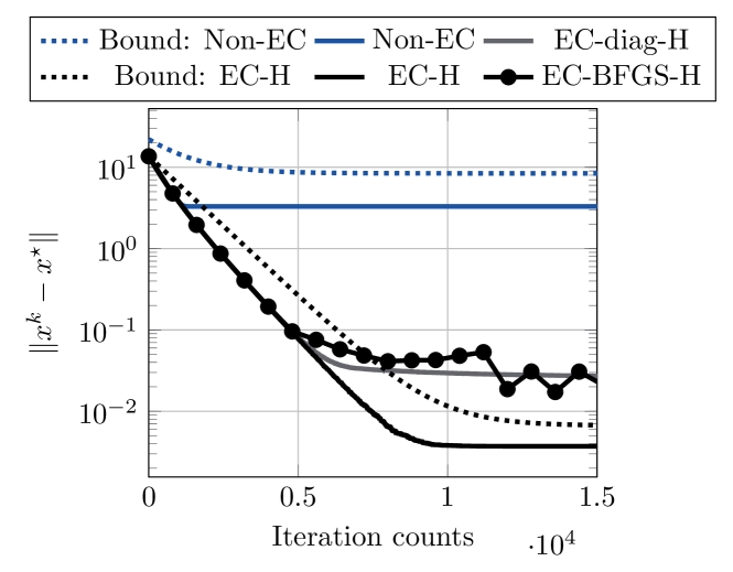
Figure 2: Comparisons of D-CSGD and D-EC-CSGD with one worker node and with $g_{i}(x;\xi_{i})=\nabla f_{i}(x)$ for the least-squares problems over synthetic data with $4,000$ data points and $400$ features, when the deterministic rounding quantizer with $\Delta=1$ is applied. We set the step-size $\gamma=2/(\mu+L)$.

We begin by considering the deterministic rounding quantizer (12). Figure 3 shows that compressed SGD cannot reach a high solution accuracy, and its performance deteriorates as the quantization resolution decreases (the compression is coarser). Error compensation, on the other hand, achieves a higher solution accuracy and is surprisingly insensitive to the amount of compression.

Figures 4 and 5 evaluate error compensation the binary (sign) compressor on several data sets in both single and multi-node settings. Almost all variants of error compensation achieve higher solution accuracy after a sufficiently large number of iterations. In particular, EC-H outperforms the other error compensation schemes in terms of high convergence speed and low residual error guarantees for centralized SGD and distributed GD. In addition, EC-diag-H has almost the same performance as EC-H.

V-B Non-convex Robust Linear Regression

Next, we consider the robust linear regression problem [32, 33], with the component function (8), $\lambda=0$ and

$$\ell(x;z_{i}^{j},y_{i}^{j})=(\langle z_{i}^{j},x\rangle-y_{i}^{j})^{2}/(1+(\langle z_{i}^{j},x\rangle-y_{i}^{j})^{2}).$$

Here, $f_{i}(\cdot)$ is smooth with $L_{i}=\sum_{j=1}^{m}\|z^{j}_{i}\|^{2}/(6\sqrt{3})$, and thus $f(\cdot)$ is smooth with the parameter $L=\max_{i\in[1,n]}L_{i}$.

We consider the binary (sign) compressor and evaluated many compensation algorithms on different data sets; see Figures 6 and 7, Compared with direct compression, almost all error compensation schemes improve the solution accuracy, and EC-H provides a higher accuracy solution than EC-diag-H and EC-I for both centralized and distributed architectures.

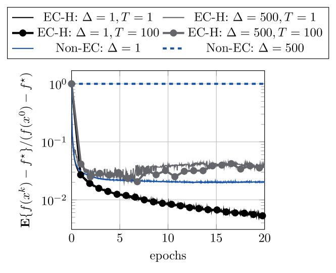
Figure 3: Comparisons of D-CSGD and D-EC-CSGD with one worker node using different compensation schemes for the least-squares problems over a3a from [34] when the deterministic rounding quantizer is applied. We set the step-size $\gamma=0.1/L$, the mini-batch size $b=|\mathcal{D}|/20$, where $|\mathcal{D}|$ is the total number of data samples.

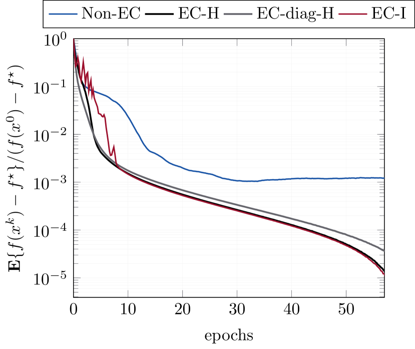
(a) mushrooms

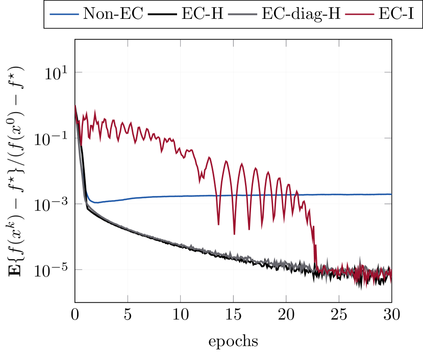
(b) a9a

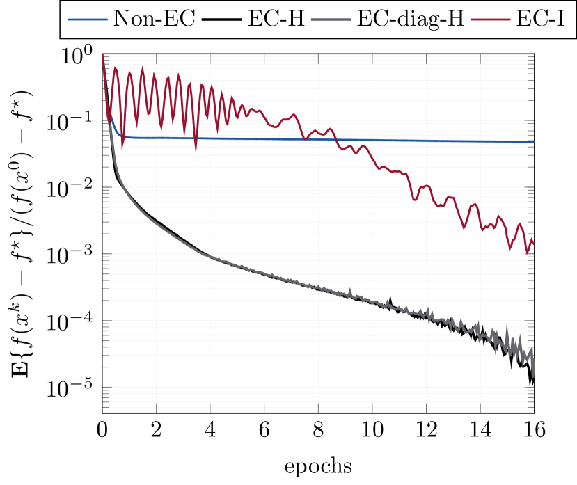
(c) w8a

Figure 4: Comparisons of D-CSGD and D-EC-CSGD with one worker node using different compensation schemes for the least-squares problems over bench-marking data sets from [34] when the binary (sign) compression is applied. We set the step-size $\gamma=0.1/L$, and the mini-batch size $b=|\mathcal{D}|/10$, where $|\mathcal{D}|$ is the total number of data samples.

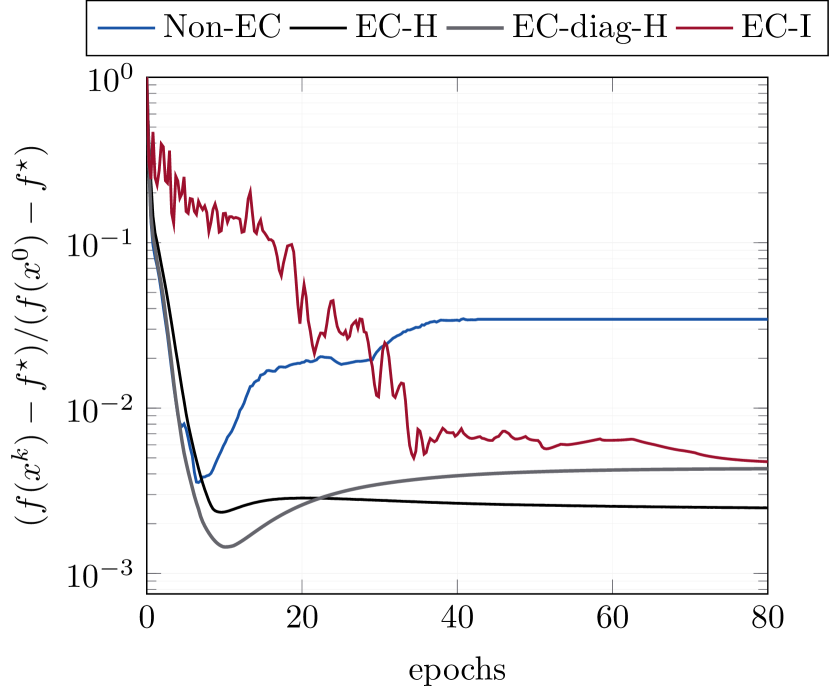
(a) mushrooms

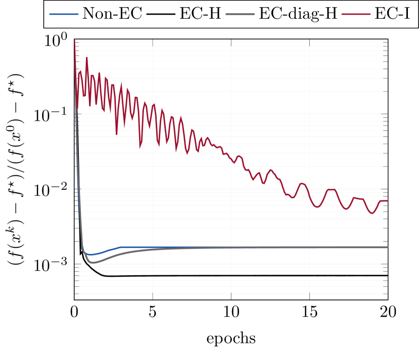
(b) a9a

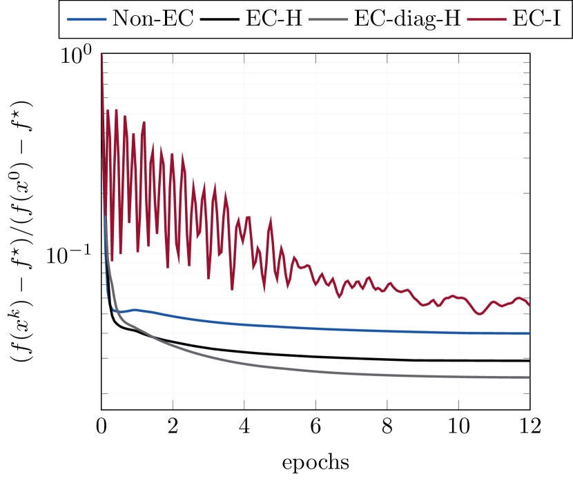
(c) w8a

Figure 5: Comparisons of D-CSGD and D-EC-CSGD with $\nabla g_{i}(x;\xi_{i})=\nabla f_{i}(x)$ using different compensation schemes for the least-squares problems over bench-marking data sets from [34] when the binary (sign) compression is applied. We set the step-size $\gamma=0.1/L$, and $5$ worker nodes.

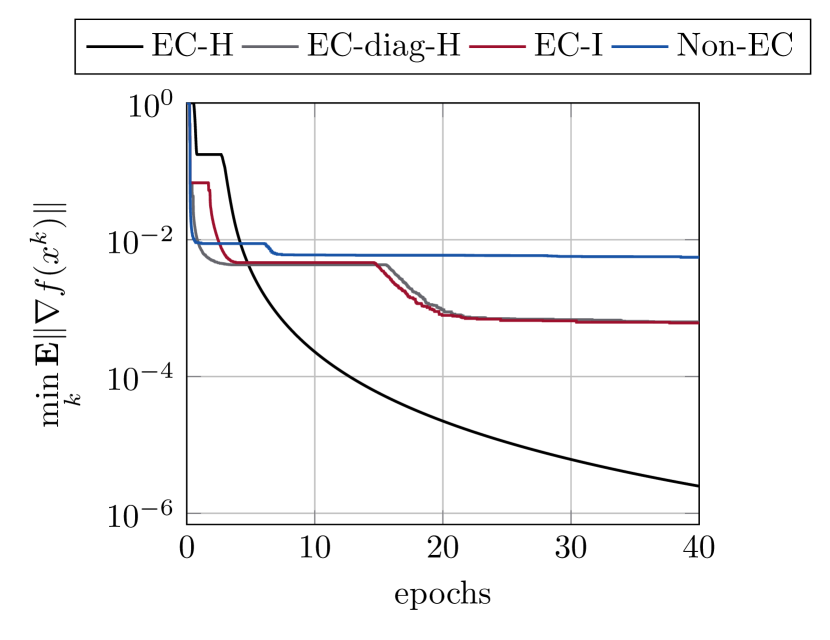
(a) a3a

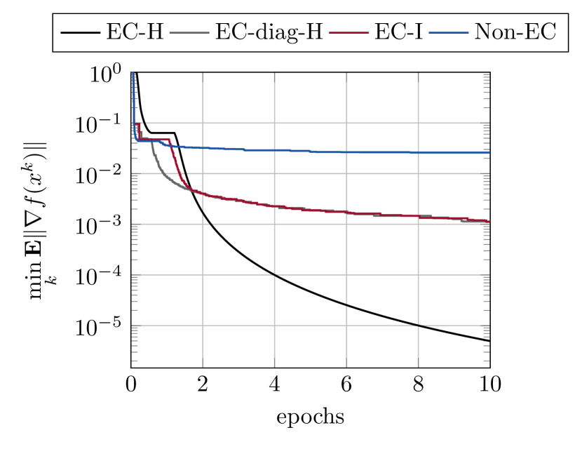
(b) mnist

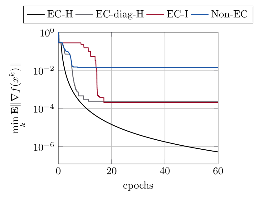
(c) phishing

Figure 6: Comparisons of D-CSGD and D-EC-CSGD with one worker node using different compensation schemes for non-convex robust linear regression over bench-marking data sets from [34] when the binary (sign) compression is applied. We set the step-size $\gamma=1/(60\sqrt{3}L)$, and the mini-batch size $b=|\mathcal{D}|/10$, where $|\mathcal{D}|$ is the total number of data samples.

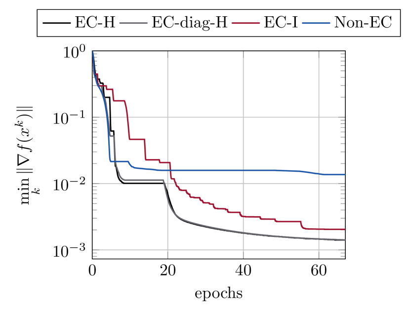
(a) a3a

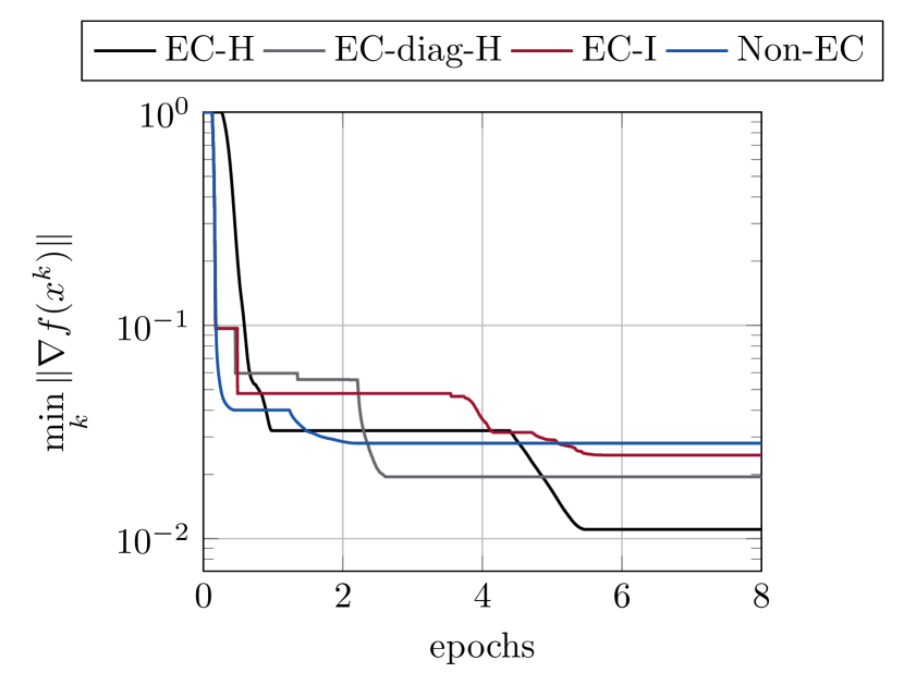
(b) mnist

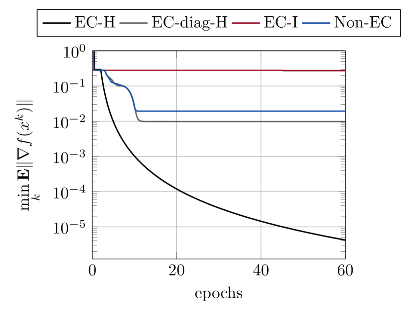
(c) phishing

Figure 7: Comparisons of D-CSGD and D-EC-CSGD with $g_{i}(x;\xi_{i})=\nabla f_{i}(x)$ using different compensation schemes for non-convex robust linear regression over bench-marking data sets from [34] when the binary (sign) compression is applied. We set the step-size $\gamma=1/(60\sqrt{3}L)$, and 5 worker nodes.

VI Conclusion

In this paper, we provided a theoretical support for error-compensation in compressed gradient methods. In particular, we showed that optimization methods with Hessian-aided error compensation can, unlike existing schemes, avoid all accumulated compression errors on quadratic problems and provide accuracy gains on ill-conditioned problems. We also provided strong convergence guarantees of Hessian-aided error-compensation for centralized and decentralized stocastic gradient methods on both convex and nonconvex problems. The superior performance of Hessian-based compensation compared to other error-compensation methods was illustrated numerically on classification problems using large benchmark data-sets in machine learning. Our experiments showed that error-compensation with diagonal Hessian approximation can achieve comparable performance as the full Hessian while saving the computational costs.

Future research directions on error compensation include the extensions for federated optimization and the use of efficient Hessian approximations. These federated optimization methods communicate compressed decision variables, rather than gradients in compressed gradient methods. Error compensation were empirically reported to improve solution accuracy of federated learning methods by initial studies in, e.g., [21, 35]. However, there is no theoretical justification which highlights the impact of error compensation on compressed decision variables and gradients. Another interesting direction is to combine Hessian approximation techniques into the error compensation. For instance, limited BFGS, which requires low storage requirements, can be used in error compensation to approximate the Hessian for solving high-dimensional and even non-smooth problems [36, 37, 38].

Appendix A Review of Useful Lemmas

This section states lemmas which are instrumental in our convergence analysis.

Lemma 1.

For $x_{i}\in\mathbb{R}^{d}$ and a natural number $N$,

$$\left\|\sum_{i=1}^{N}x_{i}\right\|^{2}\leq N\sum_{i=1}^{N}\left\|x_{i}\right\|^{2}.$$

Lemma 2.

For $x,y\in\mathbb{R}^{d}$ and a positive scalar $\theta$,

$$\left\|x+y\right\|^{2}\leq(1+\theta)\|x\|^{2}+(1+1/\theta)\|y\|^{2}.$$

Lemma 3.

For $x,y\in\mathbb{R}^{d}$ and a positive scalar $\theta$,

$$2\langle x,y\rangle\leq\theta\|x\|^{2}+(1/\theta)\|y\|^{2}.$$

Lemma 4 ([39]).

Assume that $f$ is convex and $L-$smooth, and the optimimum is denoted by $x^{\star}$. Then,

$$\|\nabla f(x)\|^{2}\leq 2L(f(x)-f(x^{\star})),\quad\text{for }x\in\mathbb{R}^{d}.$$ (29)

Appendix B Proof of Theorem 1

The algorithm in Equation (14) can be written as

$$x^{k+1}=x^{k}-\gamma(\nabla f(x^{k})+e^{k}),$$

where $e^{k}=Q(\nabla f(x^{k}))-\nabla f(x^{k})$. Using that $\nabla f(x^{\star})=Hx^{\star}-b=0$ we have

$$x^{k+1}-x^{\star}=(I-\gamma H)(x^{k}-x^{\star})-\gamma e^{k},$$

or equivalently

$$x^{k}-x^{\star}=(I-\gamma H)^{k}(x^{0}-x^{\star})-\gamma\sum_{i=0}^{k-1}(I-\gamma H)^{k-1-i}e^{i}.$$ (30)

By the triangle inequality and the fact that for a symmetric matrix $I-\gamma H$ we have

$$\|(I-\gamma H)x\|\leq\rho\|x\|\leavevmode\nobreak\ \leavevmode\nobreak\ \text{ for all }x\in\mathbb{R}^{d}.$$

where

$$\rho=\max_{i\in[1,d]}|\lambda_{i}(I-\gamma H)|=\max_{i\in[1,d]}|1-\gamma\lambda_{i}|$$

we have

$$\|x^{k}-x^{\star}\| \leq\rho^{k}\|x^{0}-x^{\star}\|+\gamma\sum_{i=0}^{k-1}\rho^{k-1-i}\epsilon.$$

In particular, when $\gamma=1/L$ then $\rho=1-1/\kappa$ meaning that

$$\|x^{k}-x^{\star}\| \leq\left(1-{1}/{\kappa}\right)^{k}\|x^{0}-x^{\star}\|$$

$$\hskip 11.38092pt+\frac{1}{L}\sum_{i=0}^{k-1}\left(1-{1}/{\kappa}\right)^{k-1-i}\epsilon,$$

where $\kappa=L/\mu$. Since $1-1/\kappa\in(0,1)$ we have

$$\sum_{i=0}^{k-1}\left(1-{1}/{\kappa}\right)^{k-1-i} \leq\sum_{i=0}^{\infty}\left(1-{1}/{\kappa}\right)^{i}=\kappa,$$

which implies

$$\|x^{k}-x^{\star}\|\leq\left(1-1/\kappa\right)^{k}\|x^{0}-x^{\star}\|+\frac{1}{\mu}\epsilon.$$

Similarly, when $\gamma=2/(\mu+L)$ then $\rho=1-2/{(\kappa+1)}$ and

$$\|x^{k}-x^{\star}\| \leq\left(1-{2}/{(\kappa+1)}\right)^{k}\|x^{0}-x^{\star}\|$$

$$\hskip 11.38092pt+\frac{2}{\mu+L}\sum_{i=0}^{k-1}\left(1-{2}/{(\kappa+1)}\right)^{k-1-i}\epsilon.$$

Since $1-2/(\kappa+1)\in(0,1)$ we have

$$\sum_{i=0}^{k-1}\left(1-{2}/{(\kappa+1)}\right)^{k-1-i} \leq\sum_{i=0}^{\infty}\left(1-{2}/{(\kappa+1)}\right)^{i}$$

$$={(\kappa+1)}/{2}.$$

This means that

$$\|x^{k}-x^{\star}\|\leq\left(\frac{\kappa-1}{\kappa+1}\right)^{k}\|x^{0}-x^{\star}\|+\frac{1}{\mu}\epsilon.$$

Appendix C Proof of Theorem 2

We can rewrite the direct compression algorithm (17) equivalently as Equation (31) with $\eta^{k}=0$. By the triangle inequality for the Euclidean norm,

$$\|x^{k+1}-x^{\star}\|\leq\|x^{k}-x^{\star}-\gamma\nabla f(x^{k})\|+\gamma\frac{1}{n}\sum_{i=1}^{n}\|e_{i}^{k}\|.$$

If $\gamma=2/(\mu+L)$, by the fact that $f(\cdot)$ is $L$-smooth and that $\|e_{i}^{k}\|\leq\epsilon$

$$\|x^{k+1}-x^{\star}\|\leq\rho\|x^{k}-x^{\star}\|+\gamma\epsilon,$$

where $\rho=1-2/(\kappa+1)$ and $\kappa=L/\mu$. By recursively applying this main inequality, we have

$$\|x^{k+1}-x^{\star}\|\leq\rho^{k}\|x^{0}-x^{\star}\|+\frac{\gamma}{1-\rho}\epsilon.$$

By rearranging the terms, we complete the proof.

Appendix D Proof of Theorem 3

We can write the algorithm in Equation (17) equivalently as

$$x^{k+1} =x^{k}-\gamma\left(\nabla f(x^{k})+\eta^{k}+e^{k}\right),$$ (31)

where

$$\eta^{k} =\frac{1}{n}\sum_{i=1}^{n}\left[g_{i}(x^{k};\xi_{i}^{k})-\nabla f_{i}(x^{k})\right],\quad\text{and}$$

$$e^{k} =\frac{1}{n}\sum_{i=1}^{n}\left[Q\left(g_{i}(x^{k};\xi_{i}^{k})\right)-g_{i}(x^{k};\xi_{i}^{k})\right].$$

By Lemma 1, the bounded gradient assumption, and the definition of the $\epsilon$-compressor we have

$$\mathbf{E}\|\eta^{k}\|^{2} \leq\frac{1}{n}\sum_{i=1}^{n}\mathbf{E}\|g_{i}(x^{k};\xi_{i}^{k})-\nabla f_{i}(x^{k})\|^{2}\leq\sigma^{2},\ \text{and}$$ (32)

$$\|e^{k}\|^{2} \leq\frac{1}{n}\sum_{i=1}^{n}\|Q\left(g_{i}(x^{k};\xi_{i}^{k})\right)-g_{i}(x^{k};\xi_{i}^{k})\|^{2}\leq\epsilon^{2}.$$ (33)

D-A Proof of Theorem 3-a)

By the Lipschitz smoothness assumption on $f(\cdot)$ and Equation (31) we have

$$f(x^{k+1}) \leq f(x^{k})-\gamma\langle\nabla f(x^{k}),\nabla f(x^{k})+\eta^{k}+e^{k}\rangle$$

$$\hskip 11.38092pt+\frac{L\gamma^{2}}{2}\|\nabla f(x^{k})+\eta^{k}+e^{k}\|^{2}.$$

Due to the unbiased property of the stochastic gradient (i.e. $\mathbf{E}\eta^{k}=0$), taking the expectation and applying Lemma 1, and Equation (32) and (33) yields

$$\mathbf{E}f(x^{k+1}) \leq\mathbf{E}f(x^{k})-\left(\gamma-\frac{3L\gamma^{2}}{2}\right)\mathbf{E}\|\nabla f(x^{k})\|^{2}$$

$$\hskip 11.38092pt+\gamma\mathbf{E}\langle\nabla f(x^{k}),-e^{k}\rangle+\frac{3L\gamma^{2}}{2}(\sigma^{2}+\epsilon^{2}).$$

Next, applying Lemma 3 with $x=\nabla f(x^{k})$, $y=-e^{k}$ and $\theta=1$ into the main result yields

$$\mathbf{E}f(x^{k+1}) \leq\mathbf{E}f(x^{k})-\left(\frac{\gamma}{2}-\frac{3L\gamma^{2}}{2}\right)\mathbf{E}\|\nabla f(x^{k})\|^{2}+T,$$

where $T=(1+3L\gamma)\gamma\epsilon^{2}/2+3L\gamma^{2}\sigma^{2}/2$. By rearranging and recalling that $\gamma<1/(3L)$ we get

$$\mathbf{E}\|\nabla f(x^{k})\|^{2} \leq\frac{2}{\gamma}\frac{1}{1-3L\gamma}\left(\mathbf{E}f(x^{k})-\mathbf{E}f(x^{k+1})+T\right).$$

Using the fact that

$$\mathop{\min}_{l\in[0,k]}\mathbf{E}\|\nabla f(x^{l})\|^{2}\leq\frac{1}{k+1}\sum_{l=0}^{k}\mathbf{E}\|\nabla f(x^{l})\|^{2}$$

and the cancelations of telescopic series we get

$$\mathop{\min}\limits_{l\in[0,k]}\mathbf{E}\|\nabla f(x^{l})\|^{2} \leq\frac{1}{k+1}\frac{2}{\gamma}\frac{1}{1-3L\gamma}\left(\mathbf{E}f(x^{0})-\mathbf{E}f(x^{k+1})\right)$$

$$\hskip 11.38092pt+\frac{2}{\gamma}\frac{1}{1-3L\gamma}T.$$

We can now conclude the proof by noting that $f(x^{\star})\leq f(x)$ for all $x\in\mathbb{R}^{d}$

D-B Proof of Theorem 3-b)

From the definition of the Euclidean norm and Equation (31),

$$\|x^{k+1}-x^{\star}\|^{2} =\|x^{k}-x^{\star}\|^{2}$$ (34)

$$\hskip 11.38092pt-2\gamma\langle\nabla f(x^{k})+\eta^{k}+e^{k},x^{k}-x^{\star}\rangle$$

$$\hskip 11.38092pt+\gamma^{2}\|\nabla f(x^{k})+\eta^{k}+e^{k}\|^{2}.$$

By taking the expected value on both sides and using the unbiasedness of the stochastic gradient, i.e., that

$$\mathbf{E}\eta^{k}=\frac{1}{n}\sum_{i=1}^{n}\mathbf{E}\left(g_{i}(x^{k};\xi_{i}^{k})-\nabla f_{i}(x^{k})\right)=0,$$

and Lemma 1 and Equation (32) and (33) to get the bound

$$\|\nabla f(x^{k})+\eta^{k}+e^{k}\|^{2}\leq 3\mathbf{E}\|\nabla f(x^{k})\|^{2}+3(\sigma^{2}+\epsilon^{2})$$

we have

$$\mathbf{E}\|x^{k+1}-x^{\star}\|^{2} \leq\mathbf{E}\|x^{k}-x^{\star}\|^{2}$$

$$\hskip 11.38092pt-2\gamma\mathbf{E}\langle\nabla f(x^{k})+e^{k},x^{k}-x^{\star}\rangle$$

$$\hskip 11.38092pt+3\gamma^{2}\mathbf{E}\|\nabla f(x^{k})\|^{2}+3\gamma^{2}(\sigma^{2}+\epsilon^{2}).$$

Applying Equation (1) with $x=x^{k}$ and $y=x^{\star}$ and using Lemma 4 with $x=x^{k}$ we have

$$\mathbf{E}\|x^{k+1}-x^{\star}\|^{2} \leq(1-\mu\gamma)\mathbf{E}\|x^{k}-x^{\star}\|^{2}$$

$$\hskip 11.38092pt-2(\gamma-3L\gamma^{2})\mathbf{E}[f(x^{k})-f(x^{\star})]$$

$$\hskip 11.38092pt+2\gamma\mathbf{E}\langle e^{k},x^{\star}-x^{k}\rangle+3\gamma^{2}(\sigma^{2}+\epsilon^{2}).$$

From Lemma 3 with $\theta=\mu$ and Equation (33), we have

$$2\gamma\langle e^{k},x^{\star}-x^{k}\rangle\leq\mu\gamma\|x^{k}-x^{\star}\|^{2}+\epsilon^{2}\gamma/\mu,$$

which yields

$$\mathbf{E}\|x^{k+1}-x^{\star}\|^{2} \leq\mathbf{E}\|x^{k}-x^{\star}\|^{2}$$

$$\hskip 11.38092pt-2\gamma(1-3L\gamma)\mathbf{E}[f(x^{k})-f(x^{\star})]+T,$$

where $T=\gamma(1/\mu+3\gamma)\epsilon^{2}+3\gamma^{2}\sigma^{2}$. By rearranging the terms and recalling that $\gamma<1/3L$ we get

$$\mathbf{E}\left(f(x^{k})-f(x^{\star})\right)$$

$$\hskip 11.38092pt\leq\frac{1}{2\gamma}\frac{1}{1-3L\gamma}\left(\mathbf{E}\|x^{k}-x^{\star}\|^{2}-\mathbf{E}\|x^{k+1}-x^{\star}\|^{2}+T\right).$$

Define $\bar{x}^{k}=\sum_{l=0}^{k}x^{l}/(k+1)$. By the convexity of $f(\cdot)$ and from the cancelations of the telescopic series we have

$$\mathbf{E}\left(f(\bar{x}^{k})-f(x^{\star})\right) \leq\frac{1}{k+1}\sum_{l=0}^{k}\mathbf{E}\left(f(x^{l})-f(x^{\star})\right)$$

$$\leq\frac{1}{k+1}\frac{1}{2\gamma}\frac{1}{1-3L\gamma}\|x^{0}-x^{\star}\|^{2}$$

$$\hskip 11.38092pt+\frac{1}{2\gamma}\frac{1}{1-3L\gamma}T.$$

Hence, the proof is complete.

Appendix E Proof of Theorem 4

We can write the algorithm in Equation (21) equivalently as

$$x^{k+1} =x^{k}-\gamma(\nabla f(x^{k})-c^{k}),$$

where

$$c^{k} =\nabla f(x^{k})-Q(\nabla f(x^{k})+A_{\gamma}e^{k}),\quad\text{and}$$

$$e^{k+1} =c^{k}+A_{\gamma}e^{k}$$

and $A_{\gamma}=I-\gamma H$. Following similar line of arguments as in the proof of Theorem 1 we obtain

$$x^{k}-x^{\star}=A_{\gamma}^{k}(x^{0}-x^{\star})+\gamma\sum_{i=0}^{k-1}A_{\gamma}^{k-1-i}c^{i}.$$

By using that $e^{k}=\sum_{i=0}^{k-1}A_{\gamma}^{k-1-i}c^{i}$ and $e^{0}=0$ we get that

$$x^{k}-x^{\star}=A_{\gamma}^{k}(x^{0}-x^{\star})+\gamma e^{k}.$$

Since $A_{\gamma}$ is symmetric, by the triangle inequality and the fact that $\|e^{k}\|\leq\epsilon$ (since $e^{k}$ is the compression error) we have

$$\|x^{k}-x^{\star}\|\leq\rho^{k}\|x^{0}-x^{\star}\|+\gamma\epsilon,$$

where $\rho=\max_{i\in[1,d]}|1-\gamma\lambda_{i}|$. Now following similar arguments as used in the proof of Theorem 1 If $\gamma=1/L$ then $\rho=1-1/\kappa$. Since $1-1/\kappa\in(0,1)$ we have

$$\|x^{k}-x^{\star}\|\leq\left(1-\frac{1}{\kappa}\right)^{k}\|x^{0}-x^{\star}\|+\frac{1}{L}\epsilon.$$

If $\gamma=2/(\mu+L)$ then $\rho=1-2/(\kappa+1)$. Since $1-2/(\kappa+1)\in(0,1)$ we have

$$\|x^{k}-x^{\star}\|\leq\left(\frac{\kappa-1}{\kappa+1}\right)^{k}\|x^{0}-x^{\star}\|+\frac{2}{\mu+L}\epsilon.$$

Appendix F Proof of Theorem 5

We can rewrite the error compensation algorithm (24) with $g_{i}(x^{k};\xi_{i}^{k})=\nabla f_{i}(x^{k})$ and $A_{i}^{k}=I-\gamma\nabla^{2}f_{i}(x^{k})$ equivalently as Equation (35) with $\eta^{k}=0$. By the triangle inequality for the Euclidean norm,

$$\|\tilde{x}^{k+1}-x^{\star}\| \leq\|\tilde{x}^{k}-x^{\star}-\gamma\nabla f(\tilde{x}^{k})\|$$

$$\hskip 11.38092pt+\gamma\|\nabla f(\tilde{x}^{k})-\nabla f(x^{k})\|$$

$$\hskip 11.38092pt+\gamma^{2}\frac{1}{n}\sum_{i=1}^{n}\|\nabla^{2}f_{i}(x^{k})e_{i}^{k}\|.$$

If $\gamma=2/(\mu+L)$, by the fact that $f(\cdot)$ is $L$-smooth and that $\tilde{x}^{k}-x^{k}=-\gamma\sum_{i=1}^{n}e_{i}^{k}/n$

$$\|\tilde{x}^{k+1}-x^{\star}\| \leq\rho\|\tilde{x}^{k}-x^{\star}\|+\gamma^{2}L\epsilon$$

$$\hskip 11.38092pt+\gamma^{2}\frac{1}{n}\sum_{i=1}^{n}\|\nabla^{2}f_{i}(x^{k})e_{i}^{k}\|,$$

where $\rho=1-2/(\kappa+1)$ and $\kappa=L/\mu$. Since each $f_{i}(\cdot)$ is $L$-smooth, $\nabla^{2}f_{i}(x)\preceq LI$ for $x\in\mathbb{R}^{d}$, and $\|e_{i}^{k}\|\leq\epsilon$, we have

$$\|\tilde{x}^{k+1}-x^{\star}\| \leq\rho\|\tilde{x}^{k}-x^{\star}\|+2\gamma^{2}L\epsilon.$$

By recursively applying this main inequality,

$$\|\tilde{x}^{k}-x^{\star}\| \leq\rho^{k}\|\tilde{x}^{0}-x^{\star}\|+\frac{2\gamma^{2}L}{1-\rho}\epsilon.$$

Using the triangle inequality and the fact that $\|x^{k}-\tilde{x}^{k}\|\leq\gamma\epsilon$, we can conclude that

$$\|x^{k}-x^{\star}\| \leq\|\tilde{x}^{k}-x^{\star}\|+\|x^{k}-\tilde{x}^{k}\|$$

$$\leq\rho^{k}\|\tilde{x}^{0}-x^{\star}\|+\left(\frac{2\gamma^{2}L}{1-\rho}+\gamma\right)\epsilon.$$

Since $\tilde{x}^{0}=x^{0}$, the proof is complete.

Appendix G Proof of Theorem 6

We can write the algorithm in Equation (24) equivalently as

$$\tilde{x}^{k+1} =\tilde{x}^{k}-\gamma\left[\nabla f(x^{k})+\eta^{k}\right]-\gamma\frac{1}{n}\sum_{i=1}^{n}(A_{i}^{k}-I)e_{i}^{k},$$ (35)

where

$$\tilde{x}^{k} =x^{k}-\gamma\frac{1}{n}\sum_{i=1}^{n}e_{i}^{k},\quad\text{and}$$

$$\eta^{k} =\frac{1}{n}\sum_{i=1}^{n}\left[\nabla g_{i}(x^{k};\xi_{i}^{k})-\nabla f_{i}(x^{k})\right].$$

By Lemma 1, the bounded gradient assumption and by the definition of the $\epsilon$-compressor, it can be proved that

$$\mathbf{E}\|\eta^{k}\|^{2} \leq\sigma^{2},\quad\text{and}$$ (36)

$$\left\|x^{k}-\tilde{x}^{k}\right\|^{2} \leq\gamma^{2}\sum_{i=1}^{n}\|e_{i}^{k}\|^{2}/n\leq\gamma^{2}\epsilon^{2}.$$ (37)

G-A Proof of Theorem 6-a)

Before deriving the main result we prove two lemmas that are need in our analysis.

Lemma 5.

Assume that $\|e_{i}^{k}\|\leq\epsilon$, and that the Hessian $H_{i}^{k}$ satisfies the unbiased and bounded variance assumptions described in Equation (27) and (28). If $\nabla^{2}f_{i}(x)\preccurlyeq LI$ for $x\in\mathbb{R}^{d}$, then

$$\mathbf{E}\left\|\gamma\frac{1}{n}\sum_{i=1}^{n}H_{i}^{k}e_{i}^{k}\right\|^{2}\leq 2\gamma^{2}(\sigma_{H}^{2}+L^{2})\epsilon^{2},\quad\text{for }k\in\mathbb{N}.$$ (38)

Proof.

By Lemma 1, we have

$$\mathbf{E}\left\|\gamma\frac{1}{n}\sum_{i=1}^{n}H_{i}^{k}e_{i}^{k}\right\|^{2} \leq 2\gamma^{2}\frac{1}{n}\sum_{i=1}^{n}\mathbf{E}\|[H_{i}^{k}-\nabla^{2}f_{i}(x^{k})]e_{i}^{k}\|^{2}$$

$$\hskip 11.38092pt+2\gamma^{2}\frac{1}{n}\sum_{i=1}^{n}\mathbf{E}\|\nabla^{2}f_{i}(x^{k})e_{i}^{k}\|^{2}.$$

Since $H_{i}^{k}-\nabla^{2}f_{i}(x^{k})$ is symmetric, using Equation (28), and the fact that $\nabla^{2}f_{i}(x^{k})\preccurlyeq LI$ and that $\|e_{i}^{k}\|\leq\epsilon$ yields

$$\mathbf{E}\left\|\gamma\frac{1}{n}\sum_{i=1}^{n}H_{i}^{k}e_{i}^{k}\right\|^{2}\leq 2\gamma^{2}(\sigma_{H}^{2}+L^{2})\epsilon^{2}.$$

∎

Lemma 6.

If $f(\cdot)$ is strongly convex, then for $\theta_{1}>0$

$$-\langle\nabla f(x^{k}),\tilde{x}^{k}-x^{\star}\rangle \leq-(f(x^{k})-f(x^{\star}))-\frac{\mu}{4}\|\tilde{x}^{k}-x^{\star}\|^{2}$$

$$\hskip 11.38092pt+\frac{1}{2}\left(\mu+\frac{1}{\theta_{1}}\right)\|\tilde{x}^{k}-x^{k}\|^{2}$$

$$\hskip 11.38092pt+\frac{\theta_{1}}{2}\|\nabla f(x^{k})\|^{2}.$$ (39)

Proof.

By using the strong convexity inequality in Equation (1) with $x=x^{k}$ and $y=x^{\star}$ we have

$$-\langle\nabla f(x^{k}),x^{k}-x^{\star}\rangle\leq-(f(x^{k})-f(x^{\star}))-\frac{\mu}{2}\|x^{k}-x^{\star}\|^{2}.$$

Using the fact that $\|x+y\|^{2}\leq 2\|x\|^{2}+2\|y\|^{2}$ with $x=x^{k}-x^{\star}$ and $y=\tilde{x}^{k}-x^{k}$, we have

$$-\|x^{k}-x^{\star}\|^{2}\leq-\frac{1}{2}\|\tilde{x}^{k}-x^{\star}\|^{2}+\|x^{k}-\tilde{x}^{k}\|^{2}.$$

Combining these inequalities yields

$$-\langle\nabla f(x^{k}),x^{k}-x^{\star}\rangle \leq-(f(x^{k})-f(x^{\star}))$$ (40)

$$\hskip 11.38092pt-\frac{\mu}{4}\|\tilde{x}^{k}-x^{\star}\|^{2}+\frac{\mu}{2}\|x^{k}-\tilde{x}^{k}\|^{2}.$$

Next, by Lemma 3

$$-\langle\nabla f(x^{k}),\tilde{x}^{k}-x^{k}\rangle\leq\frac{1}{2\theta_{1}}\|x^{k}-\tilde{x}^{k}\|^{2}+\frac{\theta_{1}}{2}\|\nabla f(x^{k})\|^{2},$$ (41)

for $\theta_{1}>0$. Summing Equation (40) and (41) completes the proof. ∎

By using the $L$-smoothness of $f(\cdot)$ and Equation (35) with $A_{i}^{k}$ defined by Equation (26) we have

$$f(\tilde{x}^{k+1}) \leq f(\tilde{x}^{k})-\gamma\langle\nabla f(\tilde{x}^{k}),\nabla f(x^{k})+\eta^{k}\rangle$$

$$\hskip 11.38092pt+\gamma\left\langle\nabla f(\tilde{x}^{k}),\gamma\frac{1}{n}\sum_{i=1}^{n}H^{k}_{i}e^{k}_{i}\right\rangle$$

$$\hskip 11.38092pt+\frac{L\gamma^{2}}{2}\left\|\nabla f(x^{k})+\eta^{k}-\gamma\frac{1}{n}\sum_{i=1}^{n}H^{k}_{i}e^{k}_{i}\right\|^{2}.$$

By the unbiased property of the stochastic gradient in Equation (10), and by applying Lemma 3 with $\theta=1$ and Lemma 1 we get

$$\mathbf{E}f(\tilde{x}^{k+1}) \leq\mathbf{E}f(\tilde{x}^{k})-\gamma\mathbf{E}\langle\nabla f(\tilde{x}^{k}),\nabla f(x^{k})\rangle$$

$$\hskip 11.38092pt+\left(\frac{\gamma}{2}+\frac{3L\gamma^{2}}{2}\right)\mathbf{E}\|\nabla f(\tilde{x}^{k})\|^{2}+\frac{3L\gamma^{2}}{2}\mathbf{E}\|\eta^{k}\|^{2}$$

$$\hskip 11.38092pt+\left(\frac{\gamma}{2}+\frac{3L\gamma^{2}}{2}\right)\mathbf{E}\left\|\gamma\frac{1}{n}\sum_{i=1}^{n}H^{k}_{i}e^{k}_{i}\right\|^{2}.$$

Since each $f_{i}(\cdot)$ is $L$-smooth, $\nabla^{2}f_{i}(x)\preceq LI$ for $x\in\mathbb{R}^{d}$. Applying the bounds in Equation (36) and (38) yields

$$\mathbf{E}f(\tilde{x}^{k+1}) \leq\mathbf{E}f(\tilde{x}^{k})-\gamma\mathbf{E}\langle\nabla f(\tilde{x}^{k}),\nabla f(x^{k})\rangle$$

$$\hskip 11.38092pt+\left(\frac{\gamma}{2}+\frac{3L\gamma^{2}}{2}\right)\mathbf{E}\|\nabla f(x^{k})\|^{2}+T,$$

where $T={3L\gamma^{2}}\sigma^{2}/2+(1+3L\gamma)(\sigma_{H}^{2}+L^{2})\gamma^{3}\epsilon^{2}.$ Using that

$$-2\langle x,y\rangle=-\|x\|^{2}-\|y\|^{2}+\|x-y\|^{2}\quad\text{for all }x,y\in\mathbb{R}^{d}$$

we have

$$\mathbf{E}f(\tilde{x}^{k+1}) \leq\mathbf{E}f(\tilde{x}^{k})-\left(\frac{\gamma}{2}-\frac{3L\gamma^{2}}{2}\right)\mathbf{E}\|\nabla f(x^{k})\|^{2}$$

$$\hskip 11.38092pt+\frac{\gamma}{2}\mathbf{E}\|\nabla f(\tilde{x}^{k})-\nabla f(x^{k})\|^{2}+T.$$

By the Lipschitz continuity assumption of $\nabla f(\cdot)$, and by (37),

$$\mathbf{E}f(\tilde{x}^{k+1}) \leq\mathbf{E}f(\tilde{x}^{k})-\left(\frac{\gamma}{2}-\frac{3L\gamma^{2}}{2}\right)\mathbf{E}\|\nabla f(x^{k})\|^{2}+\bar{T},$$

where $\bar{T}=T+L^{2}(\gamma^{3}/2)\epsilon^{2}$. By rearranging the terms and recalling that $\gamma<1/(3L)$ we get

$$\mathbf{E}\|\nabla f(x^{k})\|^{2} \leq\frac{2}{\gamma}\frac{1}{1-3L\gamma}\left(\mathbf{E}f(\tilde{x}^{k})-\mathbf{E}f(\tilde{x}^{k+1})+\bar{T}\right).$$

Since $\mathop{\min}_{l\in[0,k]}\mathbf{E}\|\nabla f(x^{l})\|^{2}\leq\sum_{l=0}^{k}\mathbf{E}\|\nabla f(x^{l})\|^{2}/(k+1)$, we have

$$\mathop{\min}\limits_{l\in[0,k]}\mathbf{E}\|\nabla f(x^{l})\|^{2} \leq\frac{1}{k+1}\frac{2}{\gamma}\frac{1}{1-3L\gamma}\left(\mathbf{E}f(\tilde{x}^{0})-\mathbf{E}f(\tilde{x}^{k+1})\right)$$

$$\hskip 11.38092pt+\frac{2}{\gamma}\frac{1}{1-3L\gamma}\bar{T}.$$

By the fact that $e^{0}=0$ (i.e. $\tilde{x}^{0}=x^{0}$), that $f(x)\geq f(x^{\star})$ for $x\in\mathbb{R}^{d}$ we complete the proof.

G-B Proof of Theorem 6-b)

From Equation (35) with $A_{i}^{k}$ defined by Equation (26) we have

$$\|\tilde{x}^{k+1}-x^{\star}\|^{2}$$

$$\hskip 11.38092pt=\|\tilde{x}^{k}-x^{\star}\|^{2}-2\gamma\langle\nabla f(x^{k})+\eta^{k},\tilde{x}^{k}-x^{\star}\rangle$$

$$\hskip 22.76228pt+2\gamma\left\langle\gamma\frac{1}{n}\sum_{i=1}^{n}H_{i}^{k}e^{k}_{i},\tilde{x}^{k}-x^{\star}\right\rangle$$

$$\hskip 22.76228pt+\gamma^{2}\left\|\nabla f(x^{k})+\eta^{k}-\gamma\frac{1}{n}\sum_{i=1}^{n}H_{i}^{k}e^{k}_{i}\right\|^{2}.$$

By the unbiasedness of the stochastic gradient described in Equation (10), by Lemma 1, by Lemma 3 with $\theta=\mu/2$ and by the bound in Equation (36) we have

$$\mathbf{E}\|\tilde{x}^{k+1}-x^{\star}\|^{2}$$

$$\hskip 11.38092pt\leq\left(1+\frac{\mu\gamma}{2}\right)\mathbf{E}\|\tilde{x}^{k}-x^{\star}\|^{2}-2\gamma\mathbf{E}\langle\nabla f(x^{k}),\tilde{x}^{k}-x^{\star}\rangle$$

$$\hskip 22.76228pt+\left(\frac{2\gamma}{\mu}+3\gamma^{2}\right)\mathbf{E}\left\|\gamma\frac{1}{n}\sum_{i=1}^{n}H_{i}^{k}e^{k}_{i}\right\|^{2}$$

$$\hskip 22.76228pt+3\gamma^{2}\mathbf{E}\|\nabla f(x^{k})\|^{2}+3\gamma^{2}\sigma^{2}.$$

Since each $f_{i}(\cdot)$ is $L$-smooth, $\nabla^{2}f_{i}(x)\preceq LI$ for $x\in\mathbb{R}^{d}$ so we can apply Lemma  6. From Equation (37) in Lemma 5 and Equation (6) in Lemma 6 with $\theta_{1}=\beta/L$ we have

$$\mathbf{E}\|\tilde{x}^{k+1}-x^{\star}\|^{2}$$

$$\hskip 11.38092pt\leq\mathbf{E}\|\tilde{x}^{k}-x^{\star}\|^{2}-2\gamma\mathbf{E}\left(f(x^{k})-f(x^{\star})\right)$$

$$\hskip 22.76228pt+\left(\frac{\beta\gamma}{L}+3\gamma^{2}\right)\mathbf{E}\|\nabla f(x^{k})\|^{2}+\bar{T},$$

where

$$\bar{T}=\left(\mu+\frac{L}{\beta}+\left(\frac{4}{\mu}+6\gamma\right)(\sigma_{H}^{2}+L^{2})\right)\gamma^{3}\epsilon^{2}+3\gamma^{2}\sigma^{2}.$$

By Lemma 4, we have

$$\mathbf{E}\|\tilde{x}^{k+1}-x^{\star}\|^{2}$$

$$\hskip 11.38092pt\leq\mathbf{E}\|\tilde{x}^{k}-x^{\star}\|^{2}-2\alpha\gamma\mathbf{E}\left(f(x^{k})-f(x^{\star})\right)+\bar{T}.$$

where $\alpha=1-\beta-3L\gamma$. By recalling that $\gamma<(1-\beta)/(3L)$ and $\beta\in(0,1)$ then

$$\mathbf{E}\left(f(x^{k})-f(x^{\star})\right)$$

$$\hskip 11.38092pt\leq\frac{1}{2\alpha\gamma}\left(\mathbf{E}\|\tilde{x}^{k}-x^{\star}\|^{2}-\mathbf{E}\|\tilde{x}^{k+1}-x^{\star}\|^{2}+\bar{T}\right).$$

Define $\bar{x}^{k}=\sum_{l=0}^{k}x^{l}/(k+1)$. By the convexity of $f(\cdot)$ and the cancelations in the telescopic series we have

$$\mathbf{E}\left(f(\bar{x}^{k})-f(x^{\star})\right) \leq\frac{1}{k+1}\sum_{l=0}^{k}\mathbf{E}\left(f(x^{l})-f(x^{\star})\right)$$

$$\leq\frac{1}{k+1}\frac{1}{2\alpha\gamma}\mathbf{E}\|\tilde{x}^{0}-x^{\star}\|^{2}+\frac{1}{2\alpha\gamma}\bar{T}.$$

By the fact that $e^{0}=0$ (i.e. $\tilde{x}^{0}=x^{0}$), the proof is complete.

References

- [1] Sarit Khirirat, Sindri Magnússon, and Mikael Johansson. Convergence bounds for compressed gradient methods with memory based error compensation. In ICASSP 2019-2019 IEEE International Conference on Acoustics, Speech and Signal Processing (ICASSP), pages 2857–2861. IEEE, 2019.
- [2] Dan Alistarh, Demjan Grubic, Jerry Li, Ryota Tomioka, and Milan Vojnovic. QSGD: Communication-efficient SGD via gradient quantization and encoding. In Advances in Neural Information Processing Systems, pages 1709–1720, 2017.
- [3] Yujun Lin, Song Han, Huizi Mao, Yu Wang, and William J Dally. Deep gradient compression: Reducing the communication bandwidth for distributed training. arXiv preprint arXiv:1712.01887, 2017.
- [4] Frank Seide, Hao Fu, Jasha Droppo, Gang Li, and Dong Yu. 1-bit stochastic gradient descent and its application to data-parallel distributed training of speech DNNs. In Fifteenth Annual Conference of the International Speech Communication Association, 2014.
- [5] Jianqiao Wangni, Jialei Wang, Ji Liu, and Tong Zhang. Gradient sparsification for communication-efficient distributed optimization. arXiv preprint arXiv:1710.09854, 2017.
- [6] Sarit Khirirat, Mikael Johansson, and Dan Alistarh. Gradient compression for communication-limited convex optimization. In 2018 IEEE Conference on Decision and Control (CDC), pages 166–171, Dec 2018.
- [7] Sindri Magnússon, Chinwendu Enyioha, Na Li, Carlo Fischione, and Vahid Tarokh. Convergence of limited communications gradient methods. IEEE Transactions on Automatic Control, 2017.
- [8] Sindri Magnússon, Hossein Shokri-Ghadikolaei, and Na Li. On maintaining linear convergence of distributed learning and optimization under limited communication. arXiv preprint arXiv:1902.11163, 2019.
- [9] Sarit Khirirat, Hamid Reza Feyzmahdavian, and Mikael Johansson. Distributed learning with compressed gradients. arXiv preprint arXiv:1806.06573, 2018.
- [10] Anastasia Koloskova, Sebastian U Stich, and Martin Jaggi. Decentralized stochastic optimization and gossip algorithms with compressed communication. arXiv preprint arXiv:1902.00340, 2019.
- [11] Thinh T Doan, Siva Theja Maguluri, and Justin Romberg. Fast convergence rates of distributed subgradient methods with adaptive quantization. arXiv preprint arXiv:1810.13245, 2018.
- [12] Amirhossein Reisizadeh, Hossein Taheri, Aryan Mokhtari, Hamed Hassani, and Ramtin Pedarsani. Robust and communication-efficient collaborative learning. In Advances in Neural Information Processing Systems, pages 8386–8397, 2019.
- [13] Xin Zhang, Jia Liu, Zhengyuan Zhu, and Elizabeth S Bentley. Compressed distributed gradient descent: Communication-efficient consensus over networks. In IEEE INFOCOM 2019-IEEE Conference on Computer Communications, pages 2431–2439. IEEE, 2019.
- [14] Amirhossein Reisizadeh, Aryan Mokhtari, Hamed Hassani, and Ramtin Pedarsani. An exact quantized decentralized gradient descent algorithm. IEEE Transactions on Signal Processing, 67(19):4934–4947, 2019.
- [15] Sai Praneeth Karimireddy, Quentin Rebjock, Sebastian U. Stich, and Martin Jaggi. Error Feedback Fixes SignSGD and other Gradient Compression Schemes. arXiv preprint arXiv:1901.09847, 2019.
- [16] Jiaxiang Wu, Weidong Huang, Junzhou Huang, and Tong Zhang. Error compensated quantized sgd and its applications to large-scale distributed optimization. arXiv preprint arXiv:1806.08054, 2018.
- [17] Nikko Strom. Scalable distributed dnn training using commodity GPU cloud computing. In Sixteenth Annual Conference of the International Speech Communication Association, 2015.
- [18] Dan Alistarh, Torsten Hoefler, Mikael Johansson, Nikola Konstantinov, Sarit Khirirat, and Cédric Renggli. The convergence of sparsified gradient methods. In Advances in Neural Information Processing Systems, pages 5977–5987, 2018.
- [19] Sebastian U Stich, Jean-Baptiste Cordonnier, and Martin Jaggi. Sparsified SGD with memory. In Advances in Neural Information Processing Systems, pages 4452–4463, 2018.
- [20] Hanlin Tang, Xiangru Lian, Tong Zhang, and Ji Liu. Doublesqueeze: Parallel stochastic gradient descent with double-pass error-compensated compression. arXiv preprint arXiv:1905.05957, 2019.
- [21] Hanlin Tang, Xiangru Lian, Shuang Qiu, Lei Yuan, Ce Zhang, Tong Zhang, and Ji Liu. DeepSqueeze: Parallel stochastic gradient descent with double-pass error-compensated compression. arXiv preprint arXiv:1907.07346, 2019.
- [22] Steven H Low and David E Lapsley. Optimization flow control—i: basic algorithm and convergence. IEEE/ACM Transactions on Networking (TON), 7(6):861–874, 1999.
- [23] Mung Chiang, Steven H Low, A Robert Calderbank, and John C Doyle. Layering as optimization decomposition: A mathematical theory of network architectures. Proceedings of the IEEE, 95(1):255–312, 2007.
- [24] Daniel Pérez Palomar and Mung Chiang. A tutorial on decomposition methods for network utility maximization. IEEE Journal on Selected Areas in Communications, 24(8):1439–1451, 2006.
- [25] Changhong Zhao, Ufuk Topcu, Na Li, and Steven Low. Design and stability of load-side primary frequency control in power systems. IEEE Transactions on Automatic Control, 59(5):1177–1189, 2014.
- [26] Sindri Magnússon, Chinwendu Enyioha, Kathryn Heal, Na Li, Carlo Fischione, and Vahid Tarokh. Distributed resource allocation using one-way communication with applications to power networks. In 2016 Annual Conference on Information Science and Systems (CISS), pages 631–636. IEEE, 2016.
- [27] Michael G Rabbat and Robert D Nowak. Quantized incremental algorithms for distributed optimization. IEEE Journal on Selected Areas in Communications, 23(4):798–808, 2005.
- [28] Shengyu Zhu, Mingyi Hong, and Biao Chen. Quantized consensus admm for multi-agent distributed optimization. In Acoustics, Speech and Signal Processing (ICASSP), 2016 IEEE International Conference on, pages 4134–4138. IEEE, 2016.
- [29] Hao Li, Soham De, Zheng Xu, Christoph Studer, Hanan Samet, and Tom Goldstein. Training quantized nets: A deeper understanding. In Advances in Neural Information Processing Systems, pages 5811–5821, 2017.
- [30] Christopher De Sa, Megan Leszczynski, Jian Zhang, Alana Marzoev, Christopher R Aberger, Kunle Olukotun, and Christopher Ré. High-accuracy low-precision training. arXiv preprint arXiv:1803.03383, 2018.
- [31] Jorge Nocedal and Stephen Wright. Numerical optimization. Springer Science & Business Media, 2006.
- [32] Peng Xu, Fred Roosta, and Michael W Mahoney. Newton-type methods for non-convex optimization under inexact hessian information. Mathematical Programming, pages 1–36, 2019.
- [33] Albert E Beaton and John W Tukey. The fitting of power series, meaning polynomials, illustrated on band-spectroscopic data. Technometrics, 16(2):147–185, 1974.
- [34] Chih-Chung Chang and Chih-Jen Lin. Libsvm: a library for support vector machines. ACM transactions on intelligent systems and technology (TIST), 2(3):27, 2011.
- [35] Debraj Basu, Deepesh Data, Can Karakus, and Suhas Diggavi. Qsparse-local-SGD: Distributed SGD with quantization, sparsification and local computations. In Advances in Neural Information Processing Systems, pages 14668–14679, 2019.
- [36] Adrian S Lewis and Michael L Overton. Nonsmooth optimization via quasi-newton methods. Mathematical Programming, 141(1-2):135–163, 2013.
- [37] Minghan Yang, Andre Milzarek, Zaiwen Wen, and Tong Zhang. A stochastic extra-step quasi-newton method for nonsmooth nonconvex optimization. arXiv preprint arXiv:1910.09373, 2019.
- [38] Lorenzo Stella, Andreas Themelis, and Panagiotis Patrinos. Forward–backward quasi-newton methods for nonsmooth optimization problems. Computational Optimization and Applications, 67(3):443–487, 2017.
- [39] Yurii Nesterov. Introductory lectures on convex optimization: A basic course, volume 87. Springer Science & Business Media, 2013.