Machine Learning Optimization
Algorithms & Portfolio Allocation

Abstract

Portfolio optimization emerged with the seminal paper of Markowitz (1952). The original mean-variance framework is appealing because it is very efficient from a computational point of view. However, it also has one well-established failing since it can lead to portfolios that are not optimal from a financial point of view (Michaud, 1989). Nevertheless, very few models have succeeded in providing a real alternative solution to the Markowitz model. The main reason lies in the fact that most academic portfolio optimization models are intractable in real life although they present solid theoretical properties. By intractable we mean that they can be implemented for an investment universe with a small number of assets using a lot of computational resources and skills, but they are unable to manage a universe with dozens or hundreds of assets. However, the emergence and the rapid development of robo-advisors means that we need to rethink portfolio optimization and go beyond the traditional mean-variance optimization approach.

Another industry and branch of science has faced similar issues concerning large-scale optimization problems. Machine learning and applied statistics have long been associated with linear and logistic regression models. Again, the reason was the inability of optimization algorithms to solve high-dimensional industrial problems. Nevertheless, the end of the 1990s marked an important turning point with the development and the rediscovery of several methods that have since produced impressive results. The goal of this paper is to show how portfolio allocation can benefit from the development of these large-scale optimization algorithms. Not all of these algorithms are useful in our case, but four of them are essential when solving complex portfolio optimization problems. These four algorithms are the coordinate descent, the alternating direction method of multipliers, the proximal gradient method and the Dykstra’s algorithm. This paper reviews them and shows how they can be implemented in portfolio allocation.

Keywords: Portfolio allocation, mean-variance optimization, risk budgeting optimization, quadratic programming, coordinate descent, alternating direction method of multipliers, proximal gradient method, Dykstra’s algorithm.

JEL classification: C61, G11.

1 Introduction

The contribution of Harry Markowitz to economics is considerable. The mean-variance optimization framework marks the beginning of portfolio allocation in finance. In addition to the seminal paper of 1952, Harry Markowitz proposed an algorithm for solving quadratic programming problems in 1956. At that time, very few people were aware of this optimization framework. We can cite Mann (1943) and Martin (1955), but it is widely accepted that Harry Markowitz is the “father of quadratic programming” (Cottle and Infanger, 2010). This is not the first time that economists are participating in the development of mathematics, but this is certainly the first time that mathematicians will explore a field of research, whose main application during the first years of research is exclusively an economic problem.

The success of mean-variance optimization (MVO) is due to the appealing properties of the quadratic utility function, but it should also be assessed in light of the success of quadratic programming (QP). Because it is easy to solve QP problems and because QP problems are available in mathematical software, solving MVO problems is straightforward and does not require a specific skill. This is why the mean-variance optimization is a universal method which is used by all portfolio managers. However, this approach has been widely criticized by academics and professionals. Indeed, mean-variance optimization is very sensitive to input parameters and produces corner solutions. Moreover, the concept of mean-variance diversification is confused with the concept of hedging (Bourgeron et al., 2018). These different issues make the practice of mean-variance optimization less attractive than the theory (Michaud, 1989). In fact, solving MVO allocation problems requires the right weight constraints to be specified in order to obtain acceptable solutions. It follows that designing the constraints is the most important component of mean-variance optimization. In this case, MVO appears to be a trial-and-error process, not a systematic solution.

The success of the MVO framework is also explained by the fact that there are very few competing portfolio allocation models that can be implemented from an industrial point of view. There are generally two reasons for this. The first one is that some models use input parameters that are difficult to estimate or understand, making these models definitively unusable. The second reason is that other models use a more complex objective function than the simple quadratic utility function. In this case, the computational complexity makes these models less attractive than the standard MVO model. Among these models, some of them are based on the mean-variance objective function, but introduce regularization penalty functions in order to improve the robustness of the portfolio allocation. Again, these models have little chance of being used if they cannot be cast into a QP problem. However, new optimization algorithms have emerged for solving large-scale machine learning problems. The purpose of this article is to present these new mathematical methods and show that they can be easily applied to portfolio allocation in order to go beyond the MVO/QP model.

This survey article is based on several previous research papers ([8], [37], [61] and [62]) and extensively uses four leading references (Beck, 2017; Boyd et al., 2010; Combettes and Pesquet, 2011; Tibshirani, 2017). It is organized as follows. In section two, we present the mean-variance approach and how it is related to the QP framework. The third section is dedicated to large-scale optimization algorithms that have been used in machine learning: coordinate descent, alternating direction method of multipliers, proximal gradient and Dykstra’s algorithm. Section four shows how these algorithms can be implemented in order to solve portfolio optimization problems and build a more robust asset allocation. Finally, section five offers some concluding remarks.

2 The quadratic programming world of portfolio optimization

2.1 Quadratic programming

2.1.1 Primal formulation

A quadratic programming (QP) problem is an optimization problem with a quadratic objective function and linear inequality constraints:

$$x^{\star} = \arg\min_{x}\frac{1}{2}x^{\top}Qx-x^{\top}R$$

s.t. $$Sx\leq T$$

where $x$ is a $n\times 1$ vector, $Q$ is a $n\times n$ matrix and $R$ is a $n\times 1$ vector. We note that the system of constraints $Sx\leq T$ allows us to specify linear equality constraints $Ax=B$ or box constraints $x^{-}\leq x\leq x^{+}$. Most numerical packages then consider the following formulation:

$$x^{\star} = \arg\min_{x}\frac{1}{2}x^{\top}Qx-x^{\top}R$$ (2)

s.t. $$\left\{\begin{array}[]{l}Ax=B\\ Cx\leq D\\ x^{-}\leq x\leq x^{+}\end{array}\right.$$ (6)

because the problem (2) is equivalent to the canonical problem (2.1.1) with the following system of linear inequalities:

$$\left[\begin{array}[]{c}-A}{\\ {\hskip 7.0pt}A}{\\ {\hskip 7.0pt}C}{\\ -I_{n}\\ {\hskip 7.0pt}I_{n}\end{array}\right]x\leq\left[\begin{array}[]{c}-B}{\\ {\hskip 7.0pt}B}{\\ {\hskip 7.0pt}D}{\\ -x^{-}\\ {\hskip 7.0pt}x^{+}\end{array}\right]$$

If the space $\Omega$ defined by $Sx\leq T$ is non-empty and if $Q$ is a symmetric positive definite matrix, the solution exists because the function $f\left(x\right)=\dfrac{1}{2}x^{\top}Qx-x^{\top}R$ is convex. In the general case where $Q$ is a square matrix, the solution may not exist.

2.1.2 Dual formulation

The Lagrange function is equal to:

$$\mathcal{L}\left(x;\lambda\right)=\frac{1}{2}x^{\top}Qx-x^{\top}R+\lambda^{\top}\left(Sx-T\right)$$

We deduce that the dual problem is defined by:

$$\lambda^{\star} = \arg\max_{\lambda}\left\{\inf_{x}\mathcal{L}\left(x;\lambda\right)\right\}$$

s.t. $$\lambda\geq 0$$

We note that $\partial_{x}\,\mathcal{L}\left(x;\lambda\right)=Qx-R+S^{\top}\lambda$. The solution to the equation $\partial_{x}\,\mathcal{L}\left(x;\lambda\right)=0$ is then $x=Q^{-1}\left(R-S^{\top}\lambda\right)$. We finally obtain:

$$\inf_{x}\mathcal{L}\left(x;\lambda\right) = \frac{1}{2}\left(R^{\top}-\lambda^{\top}S\right)Q^{-1}\left(R-S^{\top}\lambda\right)-\left(R^{\top}-\lambda^{\top}S\right)Q^{-1}R+$$

$$\lambda^{\top}\left(SQ^{-1}\left(R-S^{\top}\lambda\right)-T\right)$$

$$= \frac{1}{2}R^{\top}Q^{-1}R-\lambda^{\top}SQ^{-1}R+\frac{1}{2}\lambda^{\top}SQ^{-1}S^{\top}\lambda-R^{\top}Q^{-1}R+$$

$$2\lambda^{\top}SQ^{-1}R-\lambda^{\top}SQ^{-1}S^{\top}\lambda-\lambda^{\top}T$$

$$= -\frac{1}{2}\lambda^{\top}SQ^{-1}S^{\top}\lambda+\lambda^{\top}\left(SQ^{-1}R-T\right)-\frac{1}{2}R^{\top}Q^{-1}R$$

We deduce that the dual program is another quadratic programming problem:

$$\lambda^{\star} = \arg\min_{\lambda}\frac{1}{2}\lambda^{\top}\bar{Q}\lambda-\lambda^{\top}\bar{R}$$

s.t. $$\lambda\geq 0$$

where $\bar{Q}=SQ^{-1}S^{\top}$ and $\bar{R}=SQ^{-1}R-T$.

Remark 1

This duality property is very important for some machine learning methods. For example, this is the case of support vector machines and kernel methods that extensively use the duality for defining the solution (Cortes and Vapnik, 1995).

2.1.3 Numerical algorithms

There is a substantial literature on the methods for solving quadratic programming problems (Gould and Toint, 2000). The research begins in the 1950s with different key contributions: Frank and Wolfe (1956), Markowitz (1956), Beale (1959) and Wolfe (1959). Nowadays, QP problems are generally solved using three approaches: active set methods, gradient projection methods and interior point methods. All these algorithms are implemented in standard mathematical programming languages (Matlab, Matematica, Python, Gauss, R, etc.). This explains the success of QP problems since 2000s, because they can be easily and rapidly solved.

2.2 Mean-variance optimized portfolios

The concept of portfolio allocation has a long history and dates back to the seminal work of Markowitz (1952). In his paper, Markowitz defined precisely what portfolio selection means: “the investor does (or should) consider expected return a desirable thing and variance of return an undesirable thing”. Indeed, Markowitz showed that an efficient portfolio is the portfolio that maximizes the expected return for a given level of risk (corresponding to the variance of portfolio return) or a portfolio that minimizes the risk for a given level of expected return. Even if this framework has been extended to many other allocation problems (index sampling, turnover management, etc.), the mean-variance model remains the optimization approach that is the most widely used in finance.

2.2.1 The Markowitz framework

We consider a universe of $n$ assets. Let $x=\left(x_{1},\ldots,x_{n}\right)$ be the vector of weights in the portfolio. We assume that the portfolio is fully invested meaning that $\sum_{i=1}^{n}x_{i}=\mathbf{1}_{n}^{\top}x=1$. We denote $\mathfrak{R}=\left(\mathfrak{R}_{1},\ldots,\mathfrak{R}_{n}\right)$ as the vector of asset returns where $\mathfrak{R}_{i}$ is the return of asset $i$. The return of the portfolio is then equal to $\mathfrak{R}\left(x\right)=\sum_{i=1}^{n}x_{i}\mathfrak{R}_{i}=x^{\top}\mathfrak{R}$. Let $\mu=\mathbb{E}\left[\mathfrak{R}\right]$ and $\Sigma=\mathbb{E}\left[\left(\mathfrak{R}-\mu\right)\left(\mathfrak{R}-\mu\right)^{\top}\right]$ be the vector of expected returns and the covariance matrix of asset returns. The expected return of the portfolio is equal to:

$$\mu\left(x\right)=\mathbb{E}\left[\mathfrak{R}\left(x\right)\right]=x^{\top}\mu$$

whereas its variance is equal to:

$$\sigma^{2}\left(x\right)=\mathbb{E}\left[\left(\mathfrak{R}\left(x\right)-\mu\left(x\right)\right)\left(\mathfrak{R}\left(x\right)-\mu\left(x\right)\right)^{\top}\right]=x^{\top}\Sigma x$$

Markowitz (1952) formulated the investor’s financial problem as follows:

1. Maximizing the expected return of the portfolio under a volatility constraint ($\sigma$-problem):

   $$\max\mu\left(x\right)\quad\text{s.t.}\quad\sigma\left(x\right)\leq\sigma^{\star}$$ (8)

2. Or minimizing the volatility of the portfolio under a return constraint ($\mu$-problem):

   $$\min\sigma\left(x\right)\quad\text{s.t.}\quad\mu\left(x\right)\geq\mu^{\star}$$ (9)

Markowitz’s bright idea was to consider a quadratic utility function:

$$\mathcal{U}\left(x\right)=x^{\top}\mu-\frac{\phi}{2}x^{\top}\Sigma x$$

where $\phi\geq 0$ is the risk aversion. Since maximizing $\mathcal{U}\left(x\right)$ is equivalent to minimizing $-\mathcal{U}\left(x\right)$, the Markowitz problems (8) and (9) can be cast into a QP problem:

$$x^{\star}\left(\gamma\right) = \arg\min_{x}\frac{1}{2}x^{\top}\Sigma x-\gamma x^{\top}\mu$$

s.t. $$\mathbf{1}_{n}^{\top}x=1$$

where $\gamma=\phi^{-1}$. Therefore, solving the $\mu$-problem or the $\sigma$-problem is equivalent to finding the optimal value of $\gamma$ such that $\mu\left(x^{\star}\left(\gamma\right)\right)=\mu^{\star}$ or $\sigma\left(x^{\star}\left(\gamma\right)\right)=\sigma^{\star}$. We know that the functions $\mu\left(x^{\star}\left(\gamma\right)\right)$ and $\sigma\left(x^{\star}\left(\gamma\right)\right)$ are increasing with respect to $\gamma$ and are bounded. The optimal value of $\gamma$ can then be easily computed using the bisection algorithm. It is obvious that a large part of the success of the Markowitz framework lies on the QP trick. Indeed, Problem (2.2.1) corresponds to the QP problem (2) where $Q=\Sigma$, $R=\gamma\mu$, $A=\mathbf{1}_{n}^{\top}$ and $B=1$. Moreover, it is easy to include bounds on the weights, inequalities between asset classes, etc.

2.2.2 Solving complex MVO problems

The previous framework can be extended to other portfolio allocation problems. However, from a numerical point of view, the underlying idea is to always find an equivalent QP formulation (Roncalli, 2013).

Portfolio optimization with a benchmark

We now consider a benchmark $b$. We note $\mu\left(x\mid b\right)=\left(x-b\right)^{\top}\mu$ as the expected excess return and $\sigma\left(x\mid b\right)=\sqrt{\left(x-b\right)^{\top}\Sigma\left(x-b\right)}$ as the tracking error volatility of Portfolio $x$ with respect to Benchmark $b$. The objective function corresponds to a trade-off between minimizing the tracking error volatility and maximizing the expected excess return (or the alpha):

$$f\left(x\mid b\right)=\frac{1}{2}\sigma^{2}\left(x\mid b\right)-\gamma\mu\left(x\mid b\right)$$

We can show that the equivalent QP problem is:

$$x^{\star}\left(\gamma\right)=\arg\min_{x}\frac{1}{2}x^{\top}\Sigma x-\gamma x^{\top}\tilde{\mu}$$

where $\tilde{\mu}=\mu+\gamma^{-1}\Sigma b$ is the regularized vector of expected returns. Therefore, portfolio allocation with a benchmark can be viewed as a regularization of the MVO problem and is solved using a QP numerical algorithm.

Index sampling

The goal of index sampling is to replicate an index portfolio with a smaller number of assets than the index (or the benchmark) $b$. From a mathematical point of view, index sampling could be written as follows:

$$x^{\star} = \arg\min_{x}\frac{1}{2}\left(x-b\right)^{\top}\Sigma\left(x-b\right)$$ (11)

s.t. $$\left\{\begin{array}[]{l}\mathbf{1}_{n}^{\top}x=1\\ x\geq\mathbf{0}_{n}\\ \sum_{i=1}^{n}\mathds{1}\left\{x_{i}>0\right\}\leq n_{x}\end{array}\right.$$ (15)

The idea is to minimize the volatility of the tracking error such that the number of stocks $n_{x}$ in the portfolio is smaller than the number of stocks $n_{b}$ in the benchmark. For example, one would like to replicate the S&P 500 index with only 50 stocks and not the entire 500 stocks that compose this index. Professionals generally solve Problem (11) with the following heuristic algorithm:

1. We set $x_{\left(0\right)}^{+}=\mathbf{1}_{n}$. At the iteration $k+1$, we solve the QP problem:

   $$x^{\star} = \arg\min_{x}\frac{1}{2}\left(x-b\right)^{\top}\Sigma\left(x-b\right)$$

   s.t. $$\left\{\begin{array}[]{l}\mathbf{1}_{n}^{\top}x=1\\ \mathbf{0}_{n}\leq x\leq x_{\left(k\right)}^{+}\end{array}\right.$$

2. We then update the upper bound $x_{\left(k\right)}^{+}$ of the QP problem by deleting the asset $i^{\star}$ with the lowest non-zero optimized weight:

   $$x_{\left(k+1\right),i}^{+}\leftarrow x_{\left(k\right),i}^{+}\quad\text{if }i\neq i^{\star}\qquad\text{and}\qquad x_{\left(k+1\right),i^{\star}}^{+}\leftarrow 0$$

3. We iterate the two steps until $\sum_{i=1}^{n}\mathds{1}\left\{x_{i}^{\star}>0\right\}=n_{x}$.

The purpose of the heuristic algorithm is to delete one asset at each iteration in order to obtain an invested portfolio, which is exactly composed of $n_{x}$ assets and has a low tracking error volatility. Again, we notice that solving the index sampling problem is equivalent to solving $\left(n_{b}-n_{x}\right)$ QP problems.

Turnover management

If we note $\bar{x}$ as the current portfolio and $x$ as the new portfolio, the turnover of Portfolio $x$ with respect to Portfolio $\bar{x}$ is the sum of purchases and sales:

$$\boldsymbol{\tau}\left(x\mid\bar{x}\right)=\sum_{i=1}^{n}\left(x_{i}-\bar{x}_{i}\right)^{+}+\sum_{i=1}^{n}\left(\bar{x}_{i}-x_{i}\right)^{+}=\sum_{i=1}^{n}\left|x_{i}-\bar{x}_{i}\right|$$

Adding a turnover constraint in long-only MVO portfolios leads to the following problem:

$$x^{\star} = \arg\min_{x}\frac{1}{2}x^{\top}\Sigma x-\gamma x^{\top}\mu$$

s.t. $$\left\{\begin{array}[]{l}\sum_{i=1}^{n}x_{i}=1\\ \sum_{i=1}^{n}\left|x_{i}-\bar{x}_{i}\right|\leq\boldsymbol{\tau}^{+}\\ 0\leq x_{i}\leq 1\end{array}\right.$$

where $\boldsymbol{\tau}^{+}$ is the maximum turnover with respect to the current portfolio $\bar{x}$. Scherer (2007) introduces the additional variables $x_{i}^{-}$ and $x_{i}^{+}$ such that:

$$x_{i}=\bar{x}_{i}+x_{i}^{+}-x_{i}^{-}$$

with $x_{i}^{-}\geq 0$ indicates a negative weight change with respect to the initial weight $\bar{x}_{i}$ and $x_{i}^{+}\geq 0$ indicates a positive weight change. The expression of the turnover becomes:

$$\sum_{i=1}^{n}\left|x_{i}-\bar{x}_{i}\right|=\sum_{i=1}^{n}\left|x_{i}^{+}-x_{i}^{-}\right|=\sum_{i=1}^{n}x_{i}^{+}+\sum_{i=1}^{n}x_{i}^{-}$$

because one of the variables $x_{i}^{+}$ or $x_{i}^{-}$ is necessarily equal to zero due to the minimization problem. The $\gamma$-problem of Markowitz becomes:

$$x^{\star} = \arg\min_{x}\frac{1}{2}x^{\top}\Sigma x-\gamma x^{\top}\mu$$

s.t. $$\left\{\begin{array}[]{l}\sum_{i=1}^{n}x_{i}=1\\ x_{i}=\bar{x}_{i}+x_{i}^{+}-x_{i}^{-}\\ \sum_{i=1}^{n}x_{i}^{+}+\sum_{i=1}^{n}x_{i}^{-}\leq\boldsymbol{\tau}^{+}\\ 0\leq x_{i},x_{i}^{-},x_{i}^{+}\leq 1\end{array}\right.$$

We obtain an augmented QP problem of dimension $3n$ (see Appendix A.2 on page A.2).

Transaction costs

The previous analysis assumes that there is no transaction cost $\boldsymbol{c}\left(x\mid\bar{x}\right)$ when we rebalance the portfolio from the current portfolio $\bar{x}$ to the new optimized portfolio $x$. If we note $c_{i}^{-}$ and $c_{i}^{+}$ as the bid and ask transaction costs, we have:

$$\boldsymbol{c}\left(x\mid\bar{x}\right)=\sum_{i=1}^{n}x_{i}^{-}c_{i}^{-}+\sum_{i=1}^{n}x_{i}^{+}c_{i}^{+}$$

The net expected return of Portfolio $x$ is then equal to $\mu\left(x\right)-\boldsymbol{c}\left(x\mid\bar{x}\right)$. It follows that the $\gamma$-problem of Markowitz becomes:

$$x^{\star} = \arg\min_{x}\frac{1}{2}x^{\top}\Sigma x-\gamma\left(\sum_{i=1}^{n}x_{i}\mu_{i}-\sum_{i=1}^{n}x_{i}^{-}c_{i}^{-}-\sum_{i=1}^{n}x_{i}^{+}c_{i}^{+}\right)$$

s.t. $$\left\{\begin{array}[]{l}\sum_{i=1}^{n}x_{i}+\sum_{i=1}^{n}x_{i}^{-}c_{i}^{-}+\sum_{i=1}^{n}x_{i}^{+}c_{i}^{+}=1\\ x_{i}=\bar{x}_{i}+x_{i}^{+}-x_{i}^{-}\\ 0\leq x_{i},x_{i}^{-},x_{i}^{+}\leq 1\end{array}\right.$$

Once again, we obtain a QP problem (see Appendix A.3 on page A.3).

2.3 Issues with QP optimization

The concurrent model of the Markowitz framework is the risk budgeting approach (Qian, 2005; Maillard et al., 2010; Roncalli, 2013). The goal is to define a convex risk measure $\mathcal{R}\left(x\right)$ and to allocate the risk according to some specified risk budgets $\mathcal{RB}=\left(\mathcal{RB}_{1},\ldots,\mathcal{RB}_{n}\right)$ where $\mathcal{RB}_{i}>0$. This approach exploits the Euler decomposition property of the risk measure:

$$\mathcal{R}\left(x\right)=\sum_{i=1}^{n}x_{i}\frac{\partial\,\mathcal{R}\left(x\right)}{\partial\,x_{i}}$$

By noting $\mathcal{RC}_{i}\left(x\right)=x_{i}\cdot\partial_{x_{i}}\,\mathcal{R}\left(x\right)$ as the risk contribution of Asset $i$ with respect to portfolio $x$, the risk budgeting (RB) portfolio is defined by the following set of equations:

$$x^{\star}=\left\{x\in\left[0,1\right]^{n}:\mathcal{RC}_{i}\left(x\right)=\mathcal{RB}_{i}\right\}$$

Roncalli (2013) showed that it is equivalent to solving the following non-linear optimization problem:

$$x^{\star} = \arg\min_{x}\mathcal{R}\left(x\right)-\lambda\sum_{i=1}^{n}\mathcal{RB}_{i}\cdot\ln x_{i}$$

s.t. $$x_{i}>0$$

where $\lambda>0$ is an arbitrary positive constant. Generally, the most frequently used risk measures are the volatility risk measure (Maillard et al., 2010):

$$\mathcal{R}\left(x\right)=\sqrt{x^{\top}\Sigma x}$$

and the standard deviation-based risk measure (Roncalli, 2015):

$$\mathcal{R}\left(x\right)=-x^{\top}\left(\mu-r\right)+\xi\sqrt{x^{\top}\Sigma x}$$

where $r$ is the risk-free rate and $\xi$ is a positive scalar. In particular, this last one encompasses the Gaussian value-at-risk — $\xi=\Phi^{-1}\left(\alpha\right)$ — and the Gaussian expected shortfall — $\xi=\left(1-\alpha\right)^{-1}\phi\left(\Phi^{-1}\left(\alpha\right)\right)$.

The risk budgeting approach has displaced the MVO approach in many fields of asset management, in particular in the case of factor investing and alternative risk premia. Nevertheless, we notice that Problem (2.3) is a not a quadratic programming problem, but a logarithmic barrier problem. Therefore, the risk budgeting framework opens a new world of portfolio optimization that is not necessarily QP! That is all the more true since MVO portfolios face robustness issues (Bourgeron et al., 2018). Regularization of portfolio allocation has then become the industry standard. Indeed, it is frequent to add a $\boldsymbol{\ell}_{1}$-norm or $\boldsymbol{\ell}_{2}$-norm penalty functions to the MVO objective function. This type of penalty is, however, tractable in a quadratic programming setting. With the development of robo-advisors, non-linear penalty functions have emerged, in particular the logarithmic barrier penalty function. And these regularization techniques result in a non-quadratic programming world of portfolio optimization.

The success of this non-QP financial world will depend on how quickly and easily these complex optimization problems can be solved. Griveau-Billon at al. (2013), Bourgeron et al. (2018), and Richard and Roncalli (2019) have already proposed numerical algorithms that are doing the work in some special cases. The next section reviews the candidate algorithms that may compete with QP numerical algorithms.

3 Machine learning optimization algorithms

The machine learning industry has experienced a similar trajectory to portfolio optimization. Before the 1990s, statistical learning focused mainly on models that were easy to solve from a numerical point of view. For instance, the linear (and the ridge) regression has an analytical solution, we can solve logistic regression with the Newton-Raphson algorithm whereas supervised and unsupervised classification models consist in performing a singular value decomposition or a generalized eigenvalue decomposition. The 1990s saw the emergence of three models that have deeply changed the machine learning approach: neural networks, support vector machines and lasso regression.

Neural networks have been extensively studied since the seminal work of Rosenblatt (1958). However, the first industrial application dates back to the publication of LeCun et al. (1989) on handwritten zip code recognition. At the beginning of 1990s, a fresh craze then emerged with the writing of many handbooks that were appropriate for students, the most popular of which was Bishop (1995). With neural networks, two main issues arise concerning calibration: the large number of parameters to estimate and the absence of a global maximum. The traditional numerical optimization algorithms that were popular in the 1980s cannot be applied to neural networks. New optimization approaches are then proposed. First, researchers have considered more complex learning rules than the steepest descent (Jacobs, 1988), for example the momentum method of Polyak (1964) or the Nesterov accelerated gradient approach (Nesterov, 1983). Second, the descent method is generally not performed on the full sample of observations, but on a subset of observations that changes at each iteration. This is the underlying idea behind batch gradient descent (BGD), stochastic descent gradient (SGD) and mini-batch gradient descent (MGD). We notice that adaptive learning methods and batch optimization techniques have marked the revival of the gradient descend method.

The development of support vector machines is another important step in the development of machine learning techniques. Like neural networks, they can be seen as an extension of the perceptron. However, they present nice theoretical properties and a strong geometrical framework. Once SVMs have been first developed for linear classification, they have been extended for non-linear classification and regression. A support vector machine consists in separating hyperplanes and finding the optimal separation by maximizing the margin. The original problem called the hard margin classification can be formulated as a quadratic programming problem. However, the dual problem, which is also a QP problem, is generally preferred to the primal problem for solving SVM classification, because of the sparse property of the solution (Cortes and Vapnik, 1995). Over the years, the original hard margin classification has been extended to other problems: soft margin classification with binary hinge loss, soft margin classification with squared hinge loss, least squares SVM regression, $\varepsilon$-SVM regression, kernel machines (Vapnik, 1998). All these statistical problems share the same calibration framework. The primal problem can be cast into a QP problem, implying that the corresponding dual problem is also a QP problem. Again, we notice that the success and the prominence of statistical methods are related to the efficiency of the optimization algorithms, and it is obvious that support vector machines have substantially benefited from the QP formulation. From an industrial point of view, support vector machines present however some limitations. Indeed, if the dimension of the primal QP problem is the number $p$ of features (or parameters), the dimension of the dual QP problem is the number $n$ of observations. It is becoming absolutely impossible to solve the dual problem when the number of observations is larger than $100\,000$ and sometimes as high as several millions. This implies that new algorithms that are more appropriate for large-scale optimization problems need to be developed.

Lasso regression is the third disruptive approach that put machine learning in the spotlight in the 1990s. Like the ridge regression, lasso regression is a regularized linear regression where the $\boldsymbol{\ell}_{2}$-norm penalty is replaced by the $\boldsymbol{\ell}_{1}$-norm penalty (Tibshirani, 1996). Since the $\boldsymbol{\ell}_{1}$ regularization forces the solution to be sparse, it has been first largely used for variable selection, and then for pattern recognition and robust estimation of linear models. For finding the lasso solution, the technique of augmented QP problems is widely used since it is easy to implement. The extension of the lasso-ridge regularization to the other $\boldsymbol{\ell}_{p}$ norms is straightforward, but these approaches have never been popular. The main reason is that existing numerical algorithms are not sufficient to make these models tractable.

Therefore, the success of a quantitative model may be explained by two conditions. First, the model must be obviously appealing. Second, the model must be solved by an efficient numerical algorithm that is easy to implement or available in mathematical programming software. As shown previously, quadratic programming and gradient descent methods have been key for many statistical and financial models. In what follows, we consider four algorithms and techniques that have been popularized by their use in machine learning: coordinate descent, alternating direction method of multipliers, proximal operators and Dykstra’s algorithm. In particular, we illustrate how they can be used for solving complex optimization problems.

3.1 Coordinate descent

3.1.1 Definition

We consider the following unconstrained minimization problem:

$$x^{\star}=\arg\min_{x}f\left(x\right)$$ (21)

where $x\in\mathbb{R}^{n}$ and $f\left(x\right)$ is a continuous, smooth and convex function. A popular method to find the solution $x^{\star}$ is to consider the descent algorithm, which is defined by the following rule:

$$x^{\left(k+1\right)}=x^{\left(k\right)}+\Delta x^{\left(k\right)}=x^{\left(k\right)}-\eta D^{\left(k\right)}$$

where $x^{\left(k\right)}$ is the approximated solution of Problem (21) at the $k^{\mathrm{th}}$ Iteration, $\eta>0$ is a scalar that determines the step size and $D^{\left(k\right)}$ is the direction. We notice that the current solution $x^{\left(k\right)}$ is updated by going in the opposite direction to $D^{\left(k\right)}$ in order to obtain $x^{\left(k+1\right)}$. In the case of the gradient descent, the direction is equal to the gradient vector of $f\left(x\right)$ at the current point: $D^{\left(k\right)}=\nabla f\left(x^{\left(k\right)}\right)$. Coordinate descent (CD) is a variant of the gradient descent and minimizes the function along one coordinate at each step:

$$x_{i}^{\left(k+1\right)}=x_{i}^{\left(k\right)}+\Delta x_{i}^{\left(k\right)}=x_{i}^{\left(k\right)}-\eta D_{i}^{\left(k\right)}$$

where $D_{i}^{\left(k\right)}=\nabla_{i}f\left(x^{\left(k\right)}\right)$ is the $i^{\mathrm{th}}$ element of the gradient vector. At each iteration, a coordinate $i$ is then chosen via a certain rule, while the other coordinates are assumed to be fixed. Coordinate descent is an appealing algorithm, because it transforms a vector-valued problem into a scalar-valued problem that is easier to implement. Algorithm (1) summarizes the CD algorithm. The convergence criterion can be a predefined number of iterations or an error rule between two iterations. The step size $\eta$ can be either a given parameter or computed with a line search, implying that the parameter $\eta^{\left(k\right)}$ changes at each iteration.

  The goal is to find the solution $x^{\star}=\arg\min f\left(x\right)$

  We initialize the vector $x^{\left(0\right)}$ and we note $\eta$ the step size

  Set $k\leftarrow 0$

  repeat

     Choose a coordinate $i\in\left\{1,n\right\}$

     $x_{i}^{\left(k+1\right)}\leftarrow x_{i}^{\left(k\right)}-\eta\nabla_{i}f\left(x^{\left(k\right)}\right)$

     $x_{j}^{\left(k+1\right)}\leftarrow x_{j}^{\left(k\right)}\quad\text{if }j\neq i$

     $k\leftarrow k+1$

  until convergence

  return  $x^{\star}\leftarrow x^{\left(k\right)}$

Algorithm 1 Coordinate descent algorithm (gradient formulation)

Another formulation of the coordinate descent method is given in Algorithm (2). The underlying idea is to replace the descent approximation by the exact problem. Indeed, the objective of the descend step is to minimize the scalar-valued problem:

$$x_{i}^{\star}=\arg\min_{\varkappa}f\left(x_{1}^{\left(k\right)},\ldots,x_{i-1}^{\left(k\right)},\varkappa,x_{i+1}^{\left(k\right)},\ldots,x_{n}^{\left(k\right)}\right)$$ (22)

  The goal is to find the solution $x^{\star}=\arg\min f\left(x\right)$

  We initialize the vector $x^{\left(0\right)}$

  Set $k\leftarrow 0$

  repeat

     Choose a coordinate $i\in\left\{1,n\right\}$

     $x_{i}^{\left(k+1\right)}=\arg\min_{\varkappa}f\left(x_{1}^{\left(k\right)},\ldots,x_{i-1}^{\left(k\right)},\varkappa,x_{i+1}^{\left(k\right)},\ldots,x_{n}^{\left(k\right)}\right)$

     $x_{j}^{\left(k+1\right)}\leftarrow x_{j}^{\left(k\right)}\quad\text{if }j\neq i$

     $k\leftarrow k+1$

  until convergence

  return  $x^{\star}\leftarrow x^{\left(k\right)}$

Algorithm 2 Coordinate descent algorithm (exact formulation)

Coordinate descent is efficient in large-scale optimization problems, in particular when there is a solution to the scalar-valued problem (22). Furthermore, convergence is guaranteed when $f\left(x\right)$ is convex and differentiable (Luo and Tseng, 1992; Luo and Tseng, 1993).

Remark 2

Coordinate descent methods have been introduced in several handbooks on numerical optimization in the 1980s and 1990s (Wright, 1985). However, the most important step is the contribution of Tseng (2001), who studied the block-coordinate descent method and extended CD algorithms in the case of a non-differentiable and non-convex function $f\left(x\right)$.

3.1.2 Cyclic or random coordinates?

There are several options for choosing the coordinate of the $k^{\mathrm{th}}$ iteration. A natural choice could be to choose the coordinate which minimizes the function:

$$i^{\star}=\arg\inf\left\{f_{i}^{\star}:i\in\left\{1,n\right\},f_{i}^{\star}=\min_{\varkappa}f\left(\left(1-e_{i}\right)x^{\left(k\right)}+e_{i}\varkappa\right)\right\}$$

However, it is obvious that choosing the optimal coordinate $i^{\star}$ would require the gradient along each coordinate to be calculated. This causes the coordinate descent to be no longer efficient, since a classic gradient descent would then be of equivalent cost at each iteration and would converge faster because it requires fewer iterations.

The simplest way to implement the CD algorithm is to consider cyclic coordinates, meaning that we cyclically iterate through the coordinates (Tseng, 2001):

$$i=k\mathop{\rm mod}n$$

This ensures that all the coordinates are selected during one cycle $\left\{k-n+1,\ldots,k\right\}$ in the same order. This approach, called cyclical coordinate descent (CCD), is the most popular and used method, even if it is difficult to estimate the rate of convergence.

The second way is to consider random coordinates. Let $\pi_{i}$ be the probability of choosing the coordinate $i$ at the iteration $k$. The simplest approach is to consider uniform probabilities: $\pi_{i}=1/n$. A better approach consists in pre-specifying probabilities according to the Lipschitz constants:

$$\pi_{i}=\frac{\mathfrak{L}_{i}^{\alpha}}{\sum_{j=1}^{n}\mathfrak{L}_{j}^{\alpha}}$$ (23)

Nesterov (2012) considers three schemes: $\alpha=0$, $\alpha=1$ and $\alpha=\infty$ — in this last case, we have $i=\arg\max\left\{\mathfrak{L}_{1},\ldots,\mathfrak{L}_{n}\right\}$. From a theoretical point of view, the random coordinate descent (RCD) method based on the probability distribution (23) leads to a faster convergence, since coordinates that have a large Lipschitz constant $\mathfrak{L}_{i}$ are more likely to be chosen. However, it requires additional calculus to compute the Lipschitz constants and CCD is often preferred from a practical point of view. In what follows, we only use the CCD algorithm described below. In Algorithm (3), the variable $k$ represents the number of cycles whereas the number of iterations is equal to $k\cdot n$. For the coordinate $i$, the lower coordinates $j<i$ correspond to the current cycle $k+1$ while the upper coordinates $j>i$ correspond to the previous cycle $k$.

  The goal is to find the solution $x^{\star}=\arg\min f\left(x\right)$

  We initialize the vector $x^{\left(0\right)}$

  Set $k\leftarrow 0$

  repeat

     for $i=1:n$ do

        $x_{i}^{\left(k+1\right)}=\arg\min_{\varkappa}f\left(x_{1}^{\left(k+1\right)},\ldots,x_{i-1}^{\left(k+1\right)},\varkappa,x_{i+1}^{\left(k\right)},\ldots,x_{n}^{\left(k\right)}\right)$

     end for

     $k\leftarrow k+1$

  until convergence

  return  $x^{\star}\leftarrow x^{\left(k\right)}$

Algorithm 3 Cyclical coordinate descent algorithm

3.1.3 Application to the $\lambda$-problem of the lasso regression

We consider the linear regression:

$$Y=X\beta+\varepsilon$$ (24)

where $Y$ is the $n\times 1$ vector, $X$ is the $n\times p$ design matrix, $\beta$ is the $p\times 1$ vector of coefficients and $\varepsilon$ is the $n\times 1$ vector of residuals. In this model, $n$ is the number of observations and $p$ is the number of parameters (or the number of explanatory variables). The objective of the ordinary least squares is to minimize the residual sum of squares:

$$\hat{\beta}=\arg\min_{\beta}\frac{1}{2}\mathop{\rm RSS}\left(\beta\right)$$

where $\mathop{\rm RSS}\left(\beta\right)=\sum_{i=1}^{n}\varepsilon_{i}^{2}$. Since we have:

$$\mathop{\rm RSS}\left(\beta\right)=\left(Y-X\beta\right)^{\top}\left(Y-X\beta\right)$$

we obtain:

$$\frac{\partial\,f\left(\beta\right)}{\partial\,\beta_{j}}=-x_{j}^{\top}\left(Y-X\beta\right)$$

where $x_{j}$ is the $n\times 1$ design vector corresponding to the $j^{\mathrm{th}}$ explanatory variable. Because we can write:

$$X\beta=X_{\left(-j\right)}\beta_{\left(-j\right)}+x_{j}\beta_{j}$$

where $X_{\left(-j\right)}$ and $\beta_{\left(-j\right)}$ are the design matrix and the beta vector by excluding the $j^{\mathrm{th}}$ explanatory variable, it follows that:

$$\frac{\partial\,f\left(\beta\right)}{\partial\,\beta_{j}} = x_{j}^{\top}\left(X_{\left(-j\right)}\beta_{\left(-j\right)}+x_{j}\beta_{j}-Y\right)$$

$$= x_{j}^{\top}X_{\left(-j\right)}\beta_{\left(-j\right)}+x_{j}^{\top}x_{j}\beta_{j}-x_{j}^{\top}Y$$

At the optimum, we have $\partial_{\beta_{j}}\,f\left(\beta\right)=0$ or:

$$\beta_{j}=\frac{x_{j}^{\top}\left(Y-X_{\left(-j\right)}\beta_{\left(-j\right)}\right)}{x_{j}^{\top}x_{j}}$$ (25)

The implementation of the coordinate descent algorithm is straightforward. It suffices to iterate Equation (25) through the coordinates.

The lasso regression problem is a variant of the OLS regression by adding a $\boldsymbol{\ell}_{1}$-norm regularization (Tibshirani, 1996):

$$\hat{\beta}\left(\lambda\right)=\arg\min_{\beta}\frac{1}{2}\left(Y-X\beta\right)^{\top}\left(Y-X\beta\right)+\lambda\left\|\beta\right\|_{1}$$ (26)

In this formulation, the residual sum of squares of the linear regression is penalized by a term that will force a sparse selection of the coordinates. Since the objective function is the sum of two convex norms, the convergence is guaranteed for the lasso problem. Because $\left\|\beta\right\|_{1}=\sum_{j=1}^{n}\left|\beta_{j}\right|$, the first order condition becomes:

$$0 = \nabla_{i}f\left(\beta\right)$$

$$= x_{j}^{\top}x_{j}\beta_{j}-x_{j}^{\top}\left(Y-X_{\left(-j\right)}\beta_{\left(-j\right)}\right)+\lambda\partial\,\left|\beta_{j}\right|$$

In Appendix A.5, we show that the solution is given by:

$$\beta_{j}=\frac{\mathcal{S}\left(x_{j}^{\top}\left(Y-X_{\left(-j\right)}\beta_{\left(-j\right)}\right);\lambda\right)}{x_{j}^{\top}x_{j}}$$ (27)

where $\mathcal{S}\left(v;\lambda\right)$ is the soft-thresholding operator:

$$\mathcal{S}\left(v;\lambda\right)=\mathop{\rm sign}\left(v\right)\cdot\left(\left|v\right|-\lambda\right)_{+}$$

It follows that the lasso CD algorithm is a variation of the linear regression CD algorithm by applying the soft-threshold operator to the residuals $x_{j}^{\top}\left(Y-X_{\left(-j\right)}\beta_{\left(-j\right)}\right)$ at each iteration.

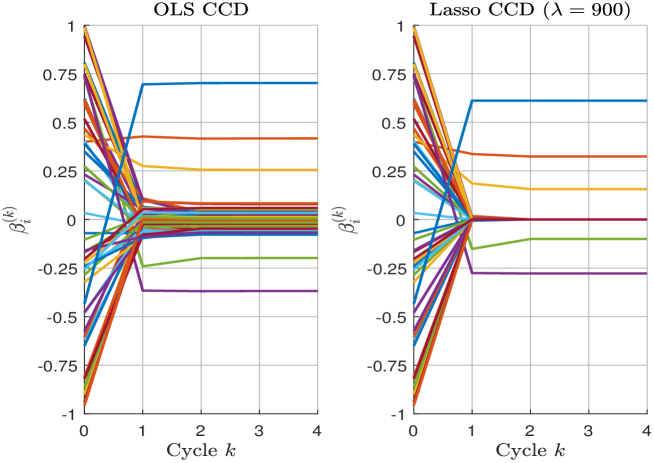
Figure 1: CCD algorithm applied to the lasso optimization problem

Let us consider an experiment with $n=10\,0000$ and $p=50$. The design matrix $X$ is built using the uniform distribution while the residuals are simulated using a Gaussian distribution and a standard deviation of $20\%$. The beta coefficients are distributed uniformly between $-3$ and $+3$ except four coefficients that take a larger value. We then standardize the data of X and Y because the practice of the lasso regression is to consider comparable beta coefficients. By considering uniform numbers between $-1$ and $+1$ for initializing the coordinates, results of the CCD algorithm are given in Figure 1. We notice that the CCD algorithm converges quickly after three complete cycles. In the case of a large-scale problem when $p\gg 1\,000$, it has been shown that CCD may be faster for the lasso regression than for the OLS regression because of the soft-thresholding operator. Indeed, we can initialize the algorithm with the null vector $\mathbf{0}_{p}$. If $\lambda$ is large, a lot of optimal coordinates are equal to zero and a few cycles are needed to find the optimal values of non-zero coefficients.

3.1.4 Application to the box-constrained QP problem

Coordinate descent can also be applied to the box-constrained QP problem:

$$x^{\star}=\arg\min_{x}\frac{1}{2}x^{\top}Qx-x^{\top}R\quad\text{s.t.}\quad x^{-}\leq x\leq x^{+}$$ (28)

In Appendix A.6 on page A.6, we show that the coordinate update of the CCD algorithm is equal to:

$$x_{i}^{\left(k+1\right)}=\mathcal{T}\left(\frac{R_{i}-\dfrac{1}{2}\sum_{j<i}x_{j}^{\left(k+1\right)}\left(Q_{i,j}+Q_{j,i}\right)-\dfrac{1}{2}\sum_{j>i}x_{j}^{\left(k\right)}\left(Q_{i,j}+Q_{j,i}\right)}{Q_{i,i}};x_{i}^{-},x_{i}^{+}\right)$$

where $\mathcal{T}\left(v;x^{-},x^{+}\right)$ is the truncation operator:

$$\mathcal{T}\left(v;x^{-},x^{+}\right) = v\odot\mathds{1}\left\{x^{-}<v<x^{+}\right\}+$$

$$x^{-}\odot\mathds{1}\left\{v\leq x^{-}\right\}+$$

$$x^{+}\odot\mathds{1}\left\{v\geq x^{+}\right\}$$

Generally, we assume that $Q$ is a symmetric matrix, implying that the CCD update reduces to:

$$x_{i}^{\left(k+1\right)}=\mathcal{T}\left(\frac{R_{i}-\sum_{j<i}x_{j}^{\left(k+1\right)}Q_{i,j}-\sum_{j>i}x_{j}^{\left(k\right)}Q_{i,j}}{Q_{i,i}};x_{i}^{-},x_{i}^{+}\right)$$

Remark 3

CCD can be applied to Problem (28) because the box constraint $x^{-}\leq x\leq x^{+}$ is pointwise.

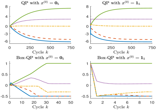
Figure 2: CCD algorithm applied to the box-constrained QP problem

We consider the following example:

$$Q=\left(\begin{array}[]{rrrrr}5.76&5.11&3.47&5.13&6.82\\ 5.11&7.98&5.38&4.30&8.70\\ 3.47&5.38&4.01&2.83&5.91\\ 5.13&4.30&2.83&4.70&5.84\\ 6.82&8.70&5.91&5.84&10.18\end{array}\right)\quad\text{and}\quad R=\left(\begin{array}[]{r}0.65\\ 0.72\\ 0.46\\ 0.59\\ 1.26\end{array}\right)$$

In Figure 2, we have reported the solution obtained with the CCD algorithm. The top panels correspond to the QP problem without any constraints, whereas the bottom panel corresponds to the QP problem with the box constraint $-0.5\leq x_{i}\leq 1$. We notice that we need more than $500$ cycles for the convergence of the CCD algorithm in the case of the unconstrained QP problem, whereas CCD finds the solution of the constrained QP problem using less than $50$ cycles. We also observe that the convergence speed is highly dependent on the starting values. In the case of the box-constrained QP problem, we need $40$ cyclical iterations if the starting value is the vector $x^{\left(0\right)}=\textbf{0}_{5}$, whereas less than $10$ cyclical iterations are sufficient if we consider the unit vector $x^{\left(0\right)}=\textbf{1}_{5}$.

3.2 Alternating direction method of multipliers

3.2.1 Definition

The alternating direction method of multipliers (ADMM) is an algorithm introduced by Gabay and Mercier (1976) to solve optimization problems which can be expressed as:

$$\left\{x^{\star},y^{\star}\right\} = \arg\min_{\left(x,y\right)}f_{x}\left(x\right)+f_{y}\left(y\right)$$

s.t. $$Ax+By=c$$

where $A\in\mathbb{R}^{p\times n}$, $B\in\mathbb{R}^{p\times m}$, $c\in\mathbb{R}^{p}$, and the functions $f_{x}:\mathbb{R}^{n}\rightarrow\mathbb{R}\cup\{+\infty\}$ and $f_{y}:\mathbb{R}^{m}\rightarrow\mathbb{R}\cup\{+\infty\}$ are proper closed convex functions. Boyd et al. (2011) show that the ADMM algorithm consists of the following three steps:

1. The $x$-update is:

   $$x^{\left(k+1\right)}=\arg\min_{x}\left\{f_{x}\left(x\right)+\frac{\varphi}{2}\left\|Ax+By^{\left(k\right)}-c+u^{\left(k\right)}\right\|_{2}^{2}\right\}$$ (31)

2. The $y$-update is:

   $$y^{\left(k+1\right)}=\arg\min_{y}\left\{f_{y}\left(y\right)+\frac{\varphi}{2}\left\|Ax^{\left(k+1\right)}+By-c+u^{\left(k\right)}\right\|_{2}^{2}\right\}$$ (32)

3. The $u$-update is:

   $$u^{\left(k+1\right)}=u^{\left(k\right)}+\left(Ax^{\left(k+1\right)}+By^{\left(k+1\right)}-c\right)$$ (33)

In this approach, $u^{\left(k\right)}$ is the dual variable of the primal residual $r=Ax+By-c$ and $\varphi$ is the $\boldsymbol{\ell}_{2}$-norm penalty variable. The parameter $\varphi$ can be constant or may change at each iteration. The ADMM algorithm benefits from the dual ascent principle and the method of multipliers. The difference with the latter is that the $x$- and $y$-updates are performed in an alternating way. Therefore, it is more flexible because the updates are equivalent to computing proximal operators for $f_{x}$ and $f_{y}$ independently. In practice, ADMM may be slow to converge with high accuracy, but is fast to converge if we consider modest accuracy. This is why ADMM is a good candidate for solving large-scale machine learning problems, where high accuracy does not necessarily lead to a better solution.

Remark 4

In this paper, we use the notations $f_{x}^{\left(k+1\right)}\left(x\right)$ and $f_{y}^{\left(k+1\right)}\left(y\right)$ when referring to the objective functions that are defined in the $x$- and $y$-updates. Algorithm (4) summarizes the different ADMM steps.

  The goal is to compute the solution $\left(x^{\star},y^{\star}\right)$

  We initialize the vectors $x^{\left(0\right)}$ and $y^{\left(0\right)}$ and we choose a value for the parameter $\varphi$

  We set $u^{\left(0\right)}=\mathbf{0}_{n}$

  $k\leftarrow 0$

  repeat

     $x^{\left(k+1\right)}=\arg\min_{x}\left\{f_{x}^{\left(k+1\right)}\left(x\right)=f_{x}\left(x\right)+\dfrac{\varphi}{2}\left\|Ax+By^{\left(k\right)}-c+u^{\left(k\right)}\right\|_{2}^{2}\right\}$

     $y^{\left(k+1\right)}=\arg\min_{y}\left\{f_{y}^{\left(k+1\right)}\left(y\right)=f_{y}\left(y\right)+\dfrac{\varphi}{2}\left\|Ax^{\left(k+1\right)}+By-c+u^{\left(k\right)}\right\|_{2}^{2}\right\}$

     $u^{\left(k+1\right)}=u^{\left(k\right)}+\left(Ax^{\left(k+1\right)}+By^{\left(k+1\right)}-c\right)$

     $k\leftarrow k+1$

  until convergence

  return  $x^{\star}\leftarrow x^{\left(k\right)}$ and $y^{\star}\leftarrow y^{\left(k\right)}$

Algorithm 4 ADMM algorithm

3.2.2 ADMM tricks

The appeal of ADMM is that it can separate a complex problem into two sub-problems that are easier to solve. However, most of the time, the optimization problem is not formulated using a separable objective function. The question is then how to formulate the initial problem as a separable problem. We now list some tricks that show how ADMM may be used in practice.

First trick

We consider a problem of the form $x^{\star}=\arg\min_{x}g\left(x\right)$. The idea is then to write $g\left(x\right)$ as a separable function $g\left(x\right)=g_{1}\left(x\right)+g_{2}\left(x\right)$ and to consider the following equivalent ADMM problem:

$$\left\{x^{\star},y^{\star}\right\} = \arg\min_{\left(x,y\right)}f_{x}\left(x\right)+f_{y}\left(y\right)$$

s.t. $$x=y$$

where $f_{x}\left(x\right)=g_{1}\left(x\right)$ and $f_{y}\left(y\right)=g_{2}\left(y\right)$. Usually, the smooth part of $g\left(x\right)$ will correspond to $g_{1}\left(x\right)$ while the non-smooth part will be included in $g_{2}\left(x\right)$. The underlying idea is that the $x$-update is straightforward, whereas the $y$-update deals with the tricky part of $g\left(x\right)$.

Second trick

If we want to minimize the function $g\left(x\right)$ where $x\in\Omega$ is a set of constraints, the optimization problem can be cast into the ADMM form (3.2.2) where $f_{x}\left(x\right)=g\left(x\right)$, $f_{y}\left(y\right)=\mathds{1}_{\Omega}\left(y\right)$ and $\mathds{1}_{\Omega}\left(x\right)$ is the convex indicator function of $\Omega$:

$$\mathds{1}_{\Omega}\left(x\right)=\left\{\begin{array}[]{lll}0&\text{if}&x\in\Omega\\ +\infty&\text{if}&x\notin\Omega\end{array}\right.$$ (35)

For example, if we want to solve the QP problem (2) given on page 2, we have:

$$f_{x}\left(x\right)=\frac{1}{2}x^{\top}Qx-x^{\top}R$$

and:

$$\Omega=\left\{x\in\mathbb{R}^{n}:Ax=B,Cx\leq D,x^{-}\leq x\leq x^{+}\right\}$$

Third trick

We can combine the first and second tricks. For instance, if we consider the following optimization problem:

$$x^{\star} = \arg\min_{x}g_{1}\left(x\right)+g_{2}\left(x\right)$$

s.t. $$x\in\Omega_{1}\cap\Omega_{2}$$

the equivalent ADMM form is:

$$\left\{x^{\star},y^{\star}\right\} = \arg\min_{\left(x,y\right)}\,\underset{f_{x}\left(x\right)}{\underbrace{\left(g_{1}\left(x\right)+\mathds{1}_{\Omega_{1}}\left(x\right)\right)}}+\underset{f_{y}\left(y\right)}{\underbrace{\left(g_{2}\left(y\right)+\mathds{1}_{\Omega_{2}}\left(y\right)\right)}}$$

s.t. $$x=y$$

Let us consider a variant of the QP problem where we add a non-linear constraint $h\left(x\right)=0$. In this case, we can write the set of constraints as $\Omega=\Omega_{1}\cap\Omega_{2}$ where:

$$\Omega_{1}=\left\{x\in\mathbb{R}^{n}:Ax=B,Cx\leq D,x^{-}\leq x\leq x^{+}\right\}$$

and:

$$\Omega_{2}=\left\{x\in\mathbb{R}^{n}:h\left(x\right)=0\right\}$$

Fourth trick

Finally, if we want to minimize the function $g\left(x\right)=g\left(x,Ax+b\right)=g_{1}\left(x\right)+g_{2}\left(Ax+b\right)$, we can write:

$$\left\{x^{\star},y^{\star}\right\} = \arg\min_{\left(x,y\right)}g_{1}\left(x\right)+g_{2}\left(y\right)$$

s.t. $$y=Ax+b$$

For instance, this trick can be used for a QP problem with a non-linear part:

$$g\left(x\right)=\frac{1}{2}x^{\top}Qx-x^{\top}R+h\left(x\right)$$

If we assume that $Q$ is a symmetric positive-definite matrix, we set $x=Ly$ where $L$ is the lower Cholesky matrix such that $LL^{\top}=Q$. It follows that the ADMM form is equal to:

$$\left\{x^{\star},y^{\star}\right\} = \arg\min_{\left(x,y\right)}\,\underset{f_{x}\left(x\right)}{\underbrace{\qquad\frac{1}{2}x^{\top}x\qquad}}+\underset{f_{y}\left(y\right)}{\underbrace{\quad\vphantom{\frac{1}{2}}h\left(y\right)-y^{\top}R\quad}}$$

s.t. $$x-Ly=\mathbf{0}_{n}$$

We notice that the $x$-update is straightforward because it corresponds to a standard QP problem. If we add a set $\Omega$ of constraints, we specify:

$$f_{y}\left(y\right)=h\left(y\right)-y^{\top}R+\mathds{1}_{\Omega}\left(y\right)$$

Remark 5

In the previous cases, we have seen that when the function $g\left(x\right)$ may contain a QP problem, it is convenient to isolate this QP problem into the $x$-update:

$$x^{\left(k+1\right)}=\arg\min_{x}\left\{\frac{1}{2}x^{\top}Qx-x^{\top}R+\mathds{1}_{\Omega}\left(x\right)+\frac{\varphi}{2}\left\|x-y^{\left(k\right)}+u^{\left(k\right)}\right\|_{2}^{2}\right\}$$

Since we have:

$$\frac{\varphi}{2}\left\|x-y^{\left(k\right)}+u^{\left(k\right)}\right\|_{2}^{2}=\frac{\varphi}{2}x^{\top}x-\varphi x^{\top}\left(y^{\left(k\right)}-u^{\left(k\right)}\right)+\frac{\varphi}{2}\left(y^{\left(k\right)}-u^{\left(k\right)}\right)^{\top}\left(y^{\left(k\right)}-u^{\left(k\right)}\right)$$

we deduce that the $x$-update is a standard QP problem where:

$$f_{x}^{\left(k+1\right)}\left(x\right)=\frac{1}{2}x^{\top}\left(Q+\varphi I_{n}\right)x-x^{\top}\left(R+\varphi\left(y^{\left(k\right)}-u^{\left(k\right)}\right)\right)+\mathds{1}_{\Omega}\left(x\right)$$ (36)

3.2.3 Application to the $\lambda$-problem of the lasso regression

The $\lambda$-problem of the lasso regression (26) has the following ADMM formulation:

$$\left\{\beta^{\star},\bar{\beta}^{\star}\right\} = \arg\min\frac{1}{2}(Y-X\beta)^{\top}(Y-X\beta)+\lambda\|\bar{\beta}\|_{1}$$

s.t. $$\beta-\bar{\beta}=\mathbf{0}_{p}$$

Since the $x$-step corresponds to a QP problem, we use the results given in Remark 5 to find the value of $\beta^{\left(k+1\right)}$:

$$\beta^{\left(k+1\right)} = \left(Q+\varphi I_{p}\right)^{-1}\left(R+\varphi\left(\bar{\beta}^{\left(k\right)}-u^{\left(k\right)}\right)\right)$$

$$= \left(X^{\top}X+\varphi I_{p}\right)^{-1}\left(X^{\top}Y+\varphi\left(\bar{\beta}^{\left(k\right)}-u^{\left(k\right)}\right)\right)$$

The $y$-step is:

$$\bar{\beta}^{\left(k+1\right)} = \arg\min_{\bar{\beta}}\left\{\lambda\|\bar{\beta}\|_{1}+\frac{\varphi}{2}\left\|\beta^{\left(k+1\right)}-\bar{\beta}+u^{\left(k\right)}\right\|_{2}^{2}\right\}$$

$$= \arg\min\left\{\frac{1}{2}\left\|\bar{\beta}-\left(\beta^{\left(k+1\right)}+u^{\left(k\right)}\right)\right\|_{2}^{2}+\frac{\lambda}{\varphi}\|\bar{\beta}\|_{1}\right\}$$

We recognize the soft-thresholding problem with $v=\beta^{\left(k+1\right)}+u^{\left(k\right)}$. Finally, the ADMM algorithm is made up of the following steps (Boyd et al., 2011):

$$\left\{\begin{array}[]{l}\beta^{\left(k+1\right)}=\left(X^{\top}X+\varphi I_{p}\right)^{-1}\left(X^{\top}Y+\varphi\left(\bar{\beta}^{\left(k\right)}-u^{\left(k\right)}\right))\right)\\ \bar{\beta}^{\left(k+1\right)}=\mathcal{S}\left(\beta^{\left(k+1\right)}+u^{\left(k\right)};\varphi^{-1}\lambda\right)\\ u^{\left(k+1\right)}=u^{\left(k\right)}+\left(\beta^{\left(k+1\right)}-\bar{\beta}^{\left(k+1\right)}\right)\end{array}\right.$$

We consider the example of the lasso regression with $\lambda=900$ on page 3.1.3. By setting $\varphi=\lambda$ and by initialing the algorithm with the OLS estimates, we obtain the convergence given in Figure 3. We notice that the ADMM algorithm converges more slowly than the CCD algorithm for this example. In practice, we generally observe that the convergence is poor for low and very high values of $\varphi$. However, finding an optimal value of $\varphi$ is difficult. A better approach involves using a varying parameter $\varphi^{\left(k\right)}$ such as the method described on page A.7.

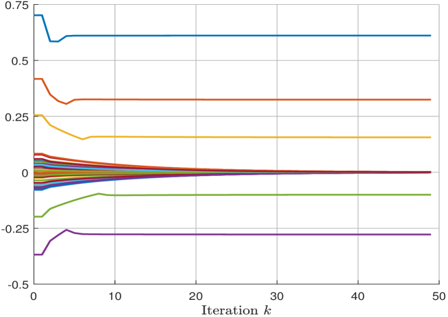
Figure 3: ADMM algorithm applied to the lasso optimization problem

3.3 Proximal operators

The $x$- and $y$-update steps of the ADMM algorithm require a $\boldsymbol{\ell}_{2}$-norm penalized optimization problem to be solved. Proximal operators are special cases of this type of problem when the matrices $A$ or $B$ correspond to the identity matrix $I_{n}$ or its opposite $-I_{n}$.

3.3.1 Definition

Let $f:\mathbb{R}^{n}\rightarrow\mathbb{R}\cup\left\{+\infty\right\}$ be a proper closed convex function. The proximal operator $\mathbf{prox}_{f}\left(v\right):\mathbb{R}^{n}\rightarrow\mathbb{R}^{n}$ is defined by:

$$\mathbf{prox}_{f}\left(v\right)=x^{\star}=\arg\min\limits_{x}\left\{f_{v}\left(x\right)=f\left(x\right)+\frac{1}{2}\left\|x-v\right\|_{2}^{2}\right\}$$ (37)

Since the function $f_{v}\left(x\right)=f\left(x\right)+\dfrac{1}{2}\left\|x-v\right\|_{2}^{2}$ is strongly convex, it has a unique minimum for every $v\in\mathbb{R}^{n}$ (Parikh and Boyd, 2014). By construction, the proximal operator defines a point $x^{\star}$ which is a trade-off between minimizing $f\left(x\right)$ and being close to $v$.

In many situations, we need to calculate the proximal of the scaled function $\lambda f\left(x\right)$ where $\lambda>0$. In this case, we use the notation $\mathbf{prox}_{\lambda f}\left(v\right)$ and we have:

$$\mathbf{prox}_{\lambda f}\left(v\right) = \arg\min\limits_{x}\left\{\lambda f\left(x\right)+\frac{1}{2}\left\|x-v\right\|_{2}^{2}\right\}$$

$$= \arg\min\limits_{x}\left\{f\left(x\right)+\frac{1}{2\lambda}\left\|x-v\right\|_{2}^{2}\right\}$$

For instance, if we consider the $y$-update of the ADMM algorithm with $B=-I_{n}$, we have:

$$y^{\left(k+1\right)} = \arg\min_{y}\left\{f_{y}\left(y\right)+\frac{\varphi}{2}\left\|y-v_{y}^{\left(k+1\right)}\right\|_{2}^{2}\right\}$$

$$= \arg\min_{y}\left\{\varphi^{-1}f_{y}\left(y\right)+\frac{1}{2}\left\|y-v_{y}^{\left(k+1\right)}\right\|_{2}^{2}\right\}$$

$$= \mathbf{prox}_{\varphi^{-1}f_{y}}\left(v_{y}^{\left(k+1\right)}\right)$$

where $v_{y}^{\left(k\right)}=Ax^{\left(k+1\right)}-c+u^{\left(k\right)}$. ADMM is then given by Algorithm (5). The interest of this mathematical formulation is to write the ADMM algorithm in a convenient form such that the $x$-update corresponds to the tricky part of the optimization while the $y$-update is reduced to an analytical formula.

  The goal is to compute the solution $\left(x^{\star},y^{\star}\right)$

  We initialize the vectors $x^{\left(0\right)}$ and $y^{\left(0\right)}$ and we choose a value for the parameter $\varphi$

  We set $u^{\left(0\right)}=\mathbf{0}_{n}$

  $k\leftarrow 0$

  repeat

     $x^{\left(k+1\right)}=\arg\min_{x}\left\{f_{x}^{\left(k+1\right)}\left(x\right)=f_{x}\left(x\right)+\dfrac{\varphi}{2}\left\|Ax-y^{\left(k\right)}-c+u^{\left(k\right)}\right\|_{2}^{2}\right\}$

     $v_{y}^{\left(k+1\right)}=Ax^{\left(k+1\right)}-c+u^{\left(k\right)}$

     $y^{\left(k+1\right)}=\mathbf{prox}_{\varphi^{-1}f_{y}}\left(v_{y}^{\left(k+1\right)}\right)$

     $u^{\left(k+1\right)}=u^{\left(k\right)}+\left(Ax^{\left(k+1\right)}-y^{\left(k+1\right)}-c\right)$

     $k\leftarrow k+1$

  until convergence

  return  $x^{\star}\leftarrow x^{\left(k\right)}$ and $y^{\star}\leftarrow y^{\left(k\right)}$

Algorithm 5 ADMM algorithm in the case $Ax-y=c$

3.3.2 Proximal operators and generalized projections

In the case where $f\left(x\right)=\mathds{1}_{\Omega}\left(x\right)$ is the indicator function, the proximal operator is then the Euclidean projection onto $\Omega$:

$$\mathbf{prox}_{f}\left(v\right) = \arg\min\limits_{x}\left\{\mathds{1}_{\Omega}\left(x\right)+\frac{1}{2}\left\|x-v\right\|_{2}^{2}\right\}$$

$$= \arg\min\limits_{x\in\Omega}\left\{\left\|x-v\right\|_{2}^{2}\right\}$$

$$= \mathcal{P}_{\Omega}\left(v\right)$$

where $\mathcal{P}_{\Omega}\left(v\right)$ is the standard projection of $v$ onto $\Omega$. Parikh and Boyd (2014) interpret then proximal operators as a generalization of the Euclidean projection.

Let us consider the constrained optimization problem $x^{\star}=\arg\min f\left(x\right)$ subject to $x\in\Omega$. Using the second ADMM trick, we have $f_{x}\left(x\right)=f\left(x\right)$, $f_{y}\left(y\right)=\mathds{1}_{\Omega}\left(y\right)$ and $x-y=\mathbf{0}_{n}$. Therefore, we can use Algorithm (5) since the $v$- and $y$-steps become $v_{y}^{\left(k+1\right)}=x^{\left(k+1\right)}+u^{\left(k\right)}$ and $y^{\left(k+1\right)}=\mathcal{P}_{\Omega}\left(v_{y}^{\left(k+1\right)}\right)$.

Here, we give the results of Parikh and Boyd (2014) for some simple polyhedra:

Notation $$\Omega$$

where $A^{\dagger}$ is the Moore-Penrose pseudo-inverse of $A$, and $\mathcal{T}\left(v;x^{-},x^{+}\right)$ is the truncation operator.

3.3.3 Main properties

There are many properties that are useful for finding the analytical expression of the proximal operator. In what follows, we consider three main properties, but the reader may refer to Combettes and Pesquet (2011), Parikh and Boyd (2014) and Beck (2017) for a more exhaustive list.

Separable sum

Let us assume that $f\left(x\right)=\sum_{i=1}^{n}f_{i}\left(x_{i}\right)$ is fully separable, then the proximal of $f\left(v\right)$ is the vector of the proximal operators applied to each scalar-valued function $f_{i}\left(x_{i}\right)$:

$$\mathbf{prox}_{f}\left(v\right)=\left(\begin{array}[]{c}\mathbf{prox}_{f_{1}}\left(v_{1}\right)\\ \vdots\\ \mathbf{prox}_{f_{n}}\left(v_{n}\right)\end{array}\right)$$

For example, if $f\left(x\right)=\lambda\left\|x\right\|_{1}$, we have $f\left(x\right)=\lambda\sum_{i=1}^{n}\left|x_{i}\right|$ and $f_{i}\left(x_{i}\right)=\lambda\left|x_{i}\right|$. We deduce that the proximal operator of $f\left(x\right)$ is the vector formulation of the soft-thresholding operator:

$$\mathbf{prox}_{\lambda\left\|x\right\|_{1}}\left(v\right)=\left(\begin{array}[]{c}\mathop{\rm sign}\left(v_{1}\right)\cdot\left(\left|v_{1}\right|-\lambda\right)_{+}\\ \vdots\\ \mathop{\rm sign}\left(v_{n}\right)\cdot\left(\left|v_{n}\right|-\lambda\right)_{+}\end{array}\right)=\mathop{\rm sign}\left(v\right)\odot\left(\left|v\right|-\lambda\mathbf{1}_{n}\right)_{+}$$

This result has been used to solve the $\lambda$-problem of the lasso regression on page 3.2.3.

If we consider the scalar-valued logarithmic barrier function $f\left(x\right)=-\lambda\ln x$, we have:

$$f_{v}\left(x\right) = -\lambda\ln x+\frac{1}{2}\left(x-v\right)^{2}$$

$$= -\lambda\ln x+\frac{1}{2}x^{2}-xv+\frac{1}{2}v^{2}$$

The first-order condition is $-\lambda x^{-1}+x-v=0$. We obtain two roots with opposite signs:

$$x^{\star}=\frac{v\pm\sqrt{v^{2}+4\lambda}}{2}$$

Since the logarithmic function is defined for $x>0$, we deduce that the proximal operator is the positive root. In the case of the vector-valued logarithmic barrier $f\left(x\right)=-\lambda\sum_{i=1}^{n}\ln x_{i}$, it follows that:

$$\mathbf{prox}_{f}(v)=\frac{v+\sqrt{v\odot v+4\lambda}}{2}$$

Moreau decomposition

An important property of the proximal operator is the Moreau decomposition theorem:

$$\mathbf{prox}_{f}\left(v\right)+\mathbf{prox}_{f^{\ast}}\left(v\right)=v$$

where $f^{\ast}$ is the convex conjugate of $f$. This result is used extensively to find the proximal of norms, the max function, the sum-of-$k$-largest-values function, etc. (Beck, 2017).

In the case of the pointwise maximum function $f\left(x\right)=\max x$, we can show that:

$$\mathbf{prox}_{\lambda\max x}\left(v\right)=\min\left(v,s^{\star}\right)$$

where $s^{\star}$ is the solution of the following equation (see Appendix A.8.1 on page A.8.1):

$$s^{\star}=\left\{s\in\mathbb{R}:\sum_{i=1}^{n}\left(v_{i}-s\right)_{+}=\lambda\right\}$$

If we assume that $f\left(x\right)=\left\|x\right\|_{p}$, we obtain:

$$p$$

If $f\left(x\right)$ is a $\boldsymbol{\ell}_{q}$-norm function, then $f^{\ast}\left(x\right)=\mathds{1}_{\mathcal{B}_{p}}\left(x\right)$ where $\mathcal{B}_{p}$ is the $\boldsymbol{\ell}_{p}$ unit ball and $p^{-1}+q^{-1}=1$. Since we have $\mathbf{prox}_{f^{\ast}}\left(v\right)=\mathcal{P}_{\mathcal{B}_{p}}\left(v\right)$, we deduce that:

$$\mathbf{prox}_{f}\left(v\right)+\mathcal{P}_{\mathcal{B}_{p}}\left(v\right)=v$$

More generally, we have:

$$\mathbf{prox}_{\lambda f}\left(v\right)+\lambda\mathcal{P}_{\mathcal{B}_{p}}\left(\frac{v}{\lambda}\right)=v$$

It follows that the projection onto the $\boldsymbol{\ell}_{p}$ ball can be deduced from the proximal operator of the $\boldsymbol{\ell}_{q}$-norm function. Let $\mathcal{B}_{p}\left(c,\lambda\right)=\left\{x\in\mathbb{R}^{n}:\left\|x-c\right\|_{p}\leq\lambda\right\}$ be the $\boldsymbol{\ell}_{p}$ ball with center $c$ and radius $\lambda$. We obtain:

$$p$$

Scaling and translation

Let us define $g\left(x\right)=f\left(ax+b\right)$ where $a\neq 0$. We have:

$$\mathbf{prox}_{g}\left(v\right)=\frac{\mathbf{prox}_{a^{2}f}\left(av+b\right)-b}{a}$$

We can use this property when the center $c$ of the $\boldsymbol{\ell}_{p}$ ball is not equal to $\mathbf{0}_{n}$. Since we have $\mathbf{prox}_{g}\left(v\right)=\mathbf{prox}_{f}\left(v-c\right)+c$ where $g\left(x\right)=f\left(x-c\right)$ and the equivalence $\mathcal{B}_{p}\left(\mathbf{0}_{n},\lambda\right)=\left\{x\in\mathbb{R}^{n}:f\left(x\right)\leq\lambda\right\}$ where $f\left(x\right)=\left\|x\right\|_{p}$, we deduce that:

$$\mathcal{P}_{\mathcal{B}_{p}\left(c,\lambda\right)}\left(v\right)=\mathcal{P}_{\mathcal{B}_{p}\left(\mathbf{0}_{n},\lambda\right)}\left(v-c\right)+c$$

3.3.4 Application to the $\tau$-problem of the lasso regression

We have previously presented the lasso regression problem by considering the Lagrange formulation ($\lambda$-problem). We now consider the original $\tau$-problem:

$$\hat{\beta}\left(\tau\right) = \arg\min_{\beta}\frac{1}{2}\left(Y-X\beta\right)^{\top}\left(Y-X\beta\right)$$

s.t. $$\left\|\beta\right\|_{1}\leq\tau$$

The ADMM formulation is:

$$\left\{\beta^{\star},\bar{\beta}^{\star}\right\} = \arg\min_{\left(\beta,\bar{\beta}\right)}\,\frac{1}{2}\left(Y-X\beta\right)^{\top}\left(Y-X\beta\right)+\mathds{1}_{\Omega}\left(\bar{\beta}\right)$$

s.t. $$\beta=\bar{\beta}$$

where $\Omega=\mathcal{B}_{1}\left(\mathbf{0}_{n},\tau\right)$ is the centered $\boldsymbol{\ell}_{1}$ ball with radius $\tau$. We notice that the $x$-update is:

$$\beta^{\left(k+1\right)} = \arg\min_{\beta}\left\{\frac{1}{2}\left(Y-X\beta\right)^{\top}\left(Y-X\beta\right)+\frac{\varphi}{2}\left\|\beta-\bar{\beta}^{\left(k\right)}+u^{\left(k\right)}\right\|_{2}^{2}\right\}$$

$$= \left(X^{\top}X+\varphi I_{p}\right)^{-1}\left(X^{\top}Y+\varphi\left(\bar{\beta}^{\left(k\right)}-u^{\left(k\right)}\right)\right)$$

where $v_{x}^{\left(k+1\right)}=\bar{\beta}^{\left(k\right)}-u^{\left(k\right)}$. For the $y$-update, we deduce that:

$$\bar{\beta}^{\left(k+1\right)} = \arg\min_{\bar{\beta}}\left\{\mathds{1}_{\Omega}\left(\bar{\beta}\right)+\frac{\varphi}{2}\left\|\beta^{\left(k+1\right)}-\bar{\beta}+u^{\left(k\right)}\right\|_{2}^{2}\right\}$$

$$= \mathbf{prox}_{f_{y}}\left(\beta^{\left(k+1\right)}+u^{\left(k\right)}\right)$$

$$= \mathcal{P}_{\Omega}\left(v_{y}^{\left(k+1\right)}\right)$$

$$= v_{y}^{\left(k+1\right)}-\mathop{\rm sign}\left(v_{y}^{\left(k+1\right)}\right)\odot\mathbf{prox}_{\tau\max x}\left(\left\|v_{y}^{\left(k+1\right)}\right\|\right)$$

where $v_{y}^{\left(k+1\right)}=\beta^{\left(k+1\right)}+u^{\left(k\right)}$. Finally, the $u$-update is defined by $u^{\left(k+1\right)}=u^{\left(k\right)}+\beta^{\left(k+1\right)}-\bar{\beta}^{\left(k+1\right)}$.

Remark 6

The ADMM algorithm is similar for $\lambda$- and $\tau$-problems since the only difference concerns the $y$-step. For the $\lambda$-problem, we apply the soft-thresholding operator while we use the $\boldsymbol{\ell}_{1}$ projection in the case of the $\tau$-problem. However, our experience shows that the $\tau$-problem is easier to solve with the ADMM algorithm from a practical point of view. The reason is that the $y$-update of the $\tau$-problem is independent of the penalization parameter $\varphi$. This is not the case for the $\lambda$-problem, because the soft-thresholding depends on the value taken by $\varphi^{-1}\lambda$.

3.3.5 Application to the CD algorithm with pointwise constraints

We consider the following constrained minimization problem:

$$x^{\star}=\arg\min_{x}f\left(x\right)\quad\text{s.t.}\quad x\in\Omega$$

where the set $\Omega$ of constraints is fully separable:

$$\mathds{1}_{\Omega}\left(x\right)=\sum_{i=1}^{n}\mathds{1}_{\Omega_{i}}\left(x_{i}\right)$$

The scalar-valued problem of the CD algorithm becomes:

$$x_{i}^{\star}=\arg\min_{\varkappa}f\left(x_{1},\ldots,x_{i-1},\varkappa,x_{i+1},\ldots,x_{n}\right)+\lambda\sum_{i=1}^{n}\mathds{1}_{\Omega_{i}}\left(x_{i}\right)$$

Nesterov (2012) and Wright (2015) propose the following coordinate update:

$$x_{i}^{\star}=\arg\min_{\varkappa}\left(\varkappa-x_{i}\right)g_{i}+\frac{1}{2\eta}\left(\varkappa-x_{i}\right)^{2}+\lambda\cdot\mathds{1}_{\Omega_{i}}\left(\varkappa\right)$$

where $g_{i}=\nabla_{i}f\left(x\right)$ is the first-derivative of the function with respect to $x_{i}$, $\eta>0$ controls the quadratic penalization term and $\lambda$ is a positive scalar. The objective function is equivalent to:

$$(\ast) = \left(\varkappa-x_{i}\right)g_{i}+\frac{1}{2\eta}\left(\varkappa-x_{i}\right)^{2}+\lambda\cdot\mathds{1}_{\Omega_{i}}\left(\varkappa\right)$$

$$= \frac{1}{2\eta}\left(\left(\varkappa-x_{i}\right)^{2}+2\left(\varkappa-x_{i}\right)\eta g_{i}\right)+\lambda\cdot\mathds{1}_{\Omega_{i}}\left(\varkappa\right)$$

$$= \frac{1}{2\eta}\left(\varkappa-x_{i}+\eta g_{i}\right)^{2}+\lambda\cdot\mathds{1}_{\Omega_{i}}\left(\varkappa\right)-\frac{\eta}{2}g_{i}^{2}$$

By taking $\lambda=\eta^{-1}$, we deduce that:

$$x_{i}^{\star} = \arg\min_{\varkappa}\mathds{1}_{\Omega_{i}}\left(\varkappa\right)+\frac{1}{2}\left\|\varkappa-\left(x_{i}-\eta g_{i}\right)\right\|^{2}$$

$$= \mathbf{prox}_{\psi}\left(x_{i}-\eta g_{i}\right)$$

$$= \mathcal{P}_{\Omega_{i}}\left(x_{i}-\eta g_{i}\right)$$

where $\psi\left(\varkappa\right)=\mathds{1}_{\Omega_{i}}\left(\varkappa\right)$. Extending the CD algorithm in the case of pointwise constraints is then equivalent to implement a standard CD algorithm and apply the projection onto the $i^{\mathrm{th}}$ coordinate at each iteration. For instance, this algorithm is particularly efficient when we consider box constraints.

3.4 Dykstra’s algorithm

We now consider the proximal optimization problem where the function $f\left(x\right)$ is the convex sum of basic functions $f_{j}\left(x\right)$:

$$x^{\star}=\arg\min_{x}\left\{\sum_{j=1}^{m}f_{j}\left(x\right)+\frac{1}{2}\left\|x-v\right\|_{2}^{2}\right\}$$

and the proximal of each basic function is known.

3.4.1 The $m=2$ case

In the previous section, we listed some analytical solutions of the proximal problem when the function $f\left(x\right)$ is basic. For instance, we know the proximal solution of the $\ell_{1}$-norm function $f_{1}\left(x\right)=\lambda_{1}\left\|x\right\|_{1}$ or the proximal solution of the logarithmic barrier function $f_{2}\left(x\right)=\lambda_{2}\sum_{i=1}^{n}\ln x_{i}$. However, we don’t know how to compute the proximal operator of $f\left(x\right)=f_{1}\left(x\right)+f_{2}\left(x\right)$:

$$x^{\star} = \arg\min_{x}f_{1}\left(x\right)+f_{2}\left(x\right)+\frac{1}{2}\left\|x-v\right\|_{2}^{2}$$

$$= \mathbf{prox}_{f}\left(v\right)$$

Nevertheless, an elegant solution is provided by the Dykstra’s algorithm (Dykstra, 1983; Bauschke and Borwein, 1994; Combettes and Pesquet, 2011), which is defined by the following iterations:

$$\left\{\begin{array}[]{l}x^{\left(k+1\right)}=\mathbf{prox}_{f_{1}}\left(y^{\left(k\right)}+p^{\left(k\right)}\right)\\ p^{\left(k+1\right)}=y^{\left(k\right)}+p^{\left(k\right)}-x^{\left(k+1\right)}\\ y^{\left(k+1\right)}=\mathbf{prox}_{f_{2}}\left(x^{\left(k+1\right)}+q^{\left(k\right)}\right)\\ q^{\left(k+1\right)}=x^{\left(k+1\right)}+q^{\left(k\right)}-y^{\left(k+1\right)}\end{array}\right.$$ (38)

where $x^{\left(0\right)}=y^{\left(0\right)}=v$ and $p^{\left(0\right)}=q^{\left(0\right)}=\mathbf{0}_{n}$. This algorithm is obviously related to the Douglas-Rachford splitting framework where $x^{\left(k\right)}$ and $p^{\left(k\right)}$ are the variable and the residual associated to $f_{1}\left(x\right)$, and $y^{\left(k\right)}$ and $q^{\left(k\right)}$ are the variable and the residual associated to $f_{2}\left(x\right)$. Algorithm (38) can be reformulated by introducing the intermediary step $k+\frac{1}{2}$:

$$\left\{\begin{array}[]{l}x^{\left(k+\frac{1}{2}\right)}=\mathbf{prox}_{f_{1}}\left(x^{\left(k\right)}+p^{\left(k\right)}\right)\\ p^{\left(k+1\right)}=p^{\left(k\right)}-\Delta_{1/2}x^{\left(k+\frac{1}{2}\right)}\\ x^{\left(k+1\right)}=\mathbf{prox}_{f_{2}}\left(x^{\left(k+\frac{1}{2}\right)}+q^{\left(k\right)}\right)\\ q^{\left(k+1\right)}=q^{\left(k\right)}-\Delta_{1/2}x^{\left(k+1\right)}\end{array}\right.$$ (39)

where $\Delta_{h}x^{\left(k\right)}=x^{\left(k\right)}-x^{\left(k-h\right)}$. Figure 4 illustrates the splitting method used by the Dykstra’s algorithm and clearly shows the relationship with the Douglas-Rachford algorithm.

Figure 4: Splitting method of the Dykstra’s algorithm

3.4.2 The $m>2$ case

The case $m>2$ is a generalization of the previous algorithm by considering $m$ residuals:

1. The $x$-update is:

   $$x^{\left(k+1\right)}=\mathbf{prox}_{f_{j\left(k\right)}}\left(x^{\left(k\right)}+z^{\left(k+1-m\right)}\right)$$

2. The $z$-update is:

   $$z^{\left(k+1\right)}=x^{\left(k\right)}+z^{\left(k+1-m\right)}-x^{\left(k+1\right)}$$

where $x^{\left(0\right)}=v$, $z^{\left(k\right)}=\mathbf{0}_{n}$ for $k<0$ and $j\left(k\right)=\mathop{\rm mod}\left(k+1,m\right)$ denotes the modulo operator taking values in $\left\{1,\ldots,m\right\}$. The variable $x^{\left(k\right)}$ is updated at each iteration while the residual $z^{\left(k\right)}$ is updated every $m$ iterations. This implies that the basic function $f_{j}\left(x\right)$ is related to the residuals $z^{\left(j\right)}$, $z^{\left(j+m\right)}$, $z^{\left(j+2m\right)}$, etc. Following Tibshirani (2017), it is better to write the Dykstra’s algorithm by using two iteration indices $k$ and $j$. The main index $k$ refers to the cycle, whereas the sub-index $j$ refers to the constraint number:

1. The $x$-update is:

   $$x^{\left(k+1,j\right)}=\mathbf{prox}_{f_{j}}\left(x^{\left(k+1,j-1\right)}+z^{\left(k,j\right)}\right)$$ (40)

2. The $z$-update is:

   $$z^{\left(k+1,j\right)}=x^{\left(k+1,j-1\right)}+z^{\left(k,j\right)}-x^{\left(k+1,j\right)}$$ (41)

where $x^{\left(1,0\right)}=v$, $z^{\left(k,j\right)}=\mathbf{0}_{n}$ for $k=0$ and $x^{\left(k+1,0\right)}=x^{\left(k,m\right)}$.

The Dykstra’s algorithm is particularly efficient when we consider the projection problem:

$$x^{\star}=\mathcal{P}_{\Omega}\left(v\right)$$

where:

$$\Omega=\Omega_{1}\cap\Omega_{2}\cap\cdots\cap\Omega_{m}$$

Indeed, the solution is found by replacing Equation (40) with:

$$x^{\left(k+1,j\right)}=\mathcal{P}_{\Omega_{j}}\left(x^{\left(k+1,j-1\right)}+z^{\left(k,j\right)}\right)$$ (42)

3.4.3 Application to general linear constraints

Let us consider the case $\Omega=\left\{x\in\mathbb{R}^{n}:Cx\leq D\right\}$ where the number of inequality constraints is equal to $m$. We can write:

$$\Omega=\Omega_{1}\cap\Omega_{2}\cap\cdots\cap\Omega_{m}$$

where $\Omega_{j}=\left\{x\in\mathbb{R}^{n}:c_{\left(j\right)}^{\top}x\leq d_{\left(j\right)}\right\}$, $c_{\left(j\right)}^{\top}$ corresponds to the $j^{\mathrm{th}}$ row of $C$ and $d_{\left(j\right)}$ is the $j^{\mathrm{th}}$ element of $D$. Since the projection $\mathcal{P}_{\Omega_{j}}$ is known and has been given on page 3.3.2, we can find the projection $\mathcal{P}_{\Omega}$ using Algorithm (6).

  The goal is to compute the solution $x^{\star}=\mathbf{prox}_{f}\left(v\right)$ where $f\left(x\right)=\mathds{1}_{\Omega}\left(x\right)$ and $\Omega=\left\{x\in\mathbb{R}^{n}:Cx\leq D\right\}$

  We initialize $x^{\left(0,m\right)}\leftarrow v$

  We set $z^{\left(0,1\right)}\leftarrow\mathbf{0}_{n},\ldots,z^{\left(0,m\right)}\leftarrow\mathbf{0}_{n}$

  $k\leftarrow 0$

  repeat

     $x^{\left(k+1,0\right)}\leftarrow x^{\left(k,m\right)}$

     for $j=1:m$ do

        The $x$-update is:

$$x^{\left(k+1,j\right)}=x^{\left(k+1,j-1\right)}+z^{\left(k,j\right)}-\frac{\left(c_{\left(j\right)}^{\top}x^{\left(k+1;j-1\right)}+c_{\left(j\right)}^{\top}z^{\left(k,j\right)}-d_{\left(j\right)}\right)_{+}}{\left\|c_{\left(j\right)}\right\|_{2}^{2}}c_{\left(j\right)}$$

        The $z$-update is:

$$z^{\left(k+1,j\right)}=x^{\left(k+1,j-1\right)}+z^{\left(k,j\right)}-x^{\left(k+1,j\right)}$$

     end for

     $k\leftarrow k+1$

  until Convergence

  return  $x^{\star}\leftarrow x^{\left(k,m\right)}$

Algorithm 6 Dykstra’s algorithm for solving the proximal problem with linear inequality constraints

If we define $\Omega$ as follows:

$$\Omega=\left\{x\in\mathbb{R}^{n}:Ax=B,Cx\leq D,x^{-}\leq x\leq x^{+}\right\}$$

we decompose $\Omega$ as the intersection of three basic convex sets:

$$\Omega=\Omega_{1}\cap\Omega_{2}\cap\Omega_{3}$$

where $\Omega_{1}=\left\{x\in\mathbb{R}^{n}:Ax=B\right\}$, $\Omega_{2}=\left\{x\in\mathbb{R}^{n}:Cx\leq D\right\}$ and $\Omega_{3}=\left\{x\in\mathbb{R}^{n}:x^{-}\leq x\leq x^{+}\right\}$. Using Dykstra’s algorithm is equivalent to formulating Algorithm (7).

  The goal is to compute the solution $x^{\star}=\mathbf{prox}_{f}\left(v\right)$ where $f\left(x\right)=\mathds{1}_{\Omega}\left(x\right)$ and $\Omega=\left\{x\in\mathbb{R}^{n}:Ax=B,Cx\leq D,x^{-}\leq x\leq x^{+}\right\}$

  We initialize $x_{m}^{\left(0\right)}\leftarrow v$

  We set $z_{1}^{\left(0\right)}\leftarrow\mathbf{0}_{n}$, $z_{2}^{\left(0\right)}\leftarrow\mathbf{0}_{n}$ and $z_{3}^{\left(0\right)}\leftarrow\mathbf{0}_{n}$

  $k\leftarrow 0$

  repeat

     $x_{0}^{\left(k+1\right)}\leftarrow x_{m}^{\left(k\right)}$

     $x_{1}^{\left(k+1\right)}\leftarrow x_{0}^{\left(k+1\right)}+z_{1}^{\left(k\right)}-A^{{\dagger}}\left(Ax_{0}^{\left(k+1\right)}+Az_{1}^{\left(k\right)}-B\right)$

     $z_{1}^{\left(k+1\right)}\leftarrow x_{0}^{\left(k+1\right)}+z_{1}^{\left(k\right)}-x_{1}^{\left(k+1\right)}$

     $x_{2}^{\left(k+1\right)}\leftarrow\mathcal{P}_{\Omega_{2}}\left(x_{1}^{\left(k+1\right)}+z_{2}^{\left(k\right)}\right)$                                     $\blacktriangleright$ Algorithm (6)

     $z_{2}^{\left(k+1\right)}\leftarrow x_{1}^{\left(k+1\right)}+z_{2}^{\left(k\right)}-x_{2}^{\left(k+1\right)}$

     $x_{3}^{\left(k+1\right)}\leftarrow\mathcal{T}\left(x_{2}^{\left(k+1\right)}+z_{3}^{\left(k\right)};x^{-},x^{+}\right)$

     $z_{3}^{\left(k+1\right)}\leftarrow x_{2}^{\left(k+1\right)}+z_{3}^{\left(k\right)}-x_{3}^{\left(k+1\right)}$

     $k\leftarrow k+1$

  until Convergence

  return  $x^{\star}\leftarrow x_{3}^{\left(k\right)}$

Algorithm 7 Dykstra’s algorithm for solving the proximal problem with general linear constraints

Since we have:

$$\frac{1}{2}\left\|x-v\right\|_{2}^{2}=\frac{1}{2}x^{\top}x-x^{\top}v+\frac{1}{2}v^{\top}v$$

we deduce that the two previous problems can be cast into a QP problem:

$$x^{\star} = \arg\min_{x}\frac{1}{2}x^{\top}I_{n}x-x^{\top}v$$

s.t. $$x\in\Omega$$

We can then compare the efficiency of Dykstra’s algorithm with the QP algorithm. Let us consider the proximal problem where the vector $v$ is defined by the elements $v_{i}=\ln\left(1+i^{2}\right)$ and the set of constraints is:

$$\Omega=\left\{x\in\mathbb{R}^{n}:\sum_{i=1}^{n}x_{i}\leq\frac{1}{2},\sum_{i=1}^{n}e^{-i}x_{i}\geq 0\right\}$$

Using a Matlab implementation, we find that the computational time of the Dykstra’s algorithm when $n$ is equal to $10$ million is equal to the QP algorithm when $n$ is equal to $12\,500$, meaning that there is a factor of $800$ between the two methods!

3.4.4 Application to the $\boldsymbol{\ell}_{2}$-penalized logarithmic barrier function

We consider the following proximal problem:

$$x^{\star} = \arg\min_{x}-\lambda\sum_{i=1}^{n}b_{i}\ln x_{i}+\frac{1}{2}\left\|x-v\right\|_{2}^{2}$$

s.t. $$\left\|x-c\right\|_{2}\leq r$$

In Appendix A.8.6 on page A.8.6, we show that the corresponding Dykstra’s algorithm is:

$$\left\{\begin{array}[]{l}x^{\left(k+1\right)}=\dfrac{y^{\left(k\right)}+z_{1}^{\left(k\right)}+\sqrt{\left(y^{\left(k\right)}+z_{1}^{\left(k\right)}\right)\odot\left(y^{\left(k\right)}+z_{1}^{\left(k\right)}\right)+4\lambda b}}{2}\\ z_{1}^{\left(k+1\right)}=y^{\left(k\right)}+z_{1}^{\left(k\right)}-x^{\left(k+1\right)}\\ y^{\left(k+1\right)}=c+\dfrac{r}{\max\left(r,\left\|x^{\left(k+1\right)}+z_{2}^{\left(k\right)}-c\right\|_{2}\right)}\left(x^{\left(k+1\right)}+z_{2}^{\left(k\right)}-c\right)\\ z_{2}^{\left(k+1\right)}=x^{\left(k+1\right)}+z_{2}^{\left(k\right)}-y^{\left(k+1\right)}\end{array}\right.$$

4 Applications to portfolio optimization

The development of the previous algorithms will fundamentally change the practice of portfolio optimization. Until now, we have seen that portfolio managers live in a quadratic programming world. With these new optimization algorithms, we can consider more complex portfolio optimization programs with non-quadratic objective function, regularization with penalty functions and non-linear constraints.

Table 1: Some objective functions used in portfolio optimization

Item	Portfolio	$f\left(x\right)$	Reference
(1)	MVO	$\frac{1}{2}x^{\top}\Sigma x-\gamma x^{\top}\mu$	Markowitz (1952)
(2)	GMV	$\frac{1}{2}x^{\top}\Sigma x$	Jagganathan and Ma (2003)
(3)	MDP	$\ln\left(\sqrt{x^{\top}\Sigma x}\right)-\ln\left(x^{\top}\sigma\right)$	Choueifaty and Coignard (2008)
(4)	KL	$\sum_{i=1}^{n}x_{i}\ln\left(x_{i}/\tilde{x}_{i}\right)$	Bera and Park (2008)
(5)	ERC	$\frac{1}{2}x^{\top}\Sigma x-\lambda\sum_{i=1}^{n}\ln x_{i}$	Maillard et al. (2010)
(6)	RB	$\mathcal{R}\left(x\right)-\lambda\sum_{i=1}^{n}\mathcal{RB}_{i}\cdot\ln x_{i}$	Roncalli (2015)
(7)	RQE	$\frac{1}{2}x^{\top}Dx$	Carmichael et al. (2018)

We consider a universe of $n$ assets. Let $x$ be the vector of weights in the portfolio. We denote by $\mu$ and $\Sigma$ the vector of expected returns and the covariance matrix of asset returns. Some models consider also a reference portfolio $\tilde{x}$. In Table 1, we report the main objective functions that are used by professionals. Besides the mean-variance optimized portfolio (MVO) and the global minimum variance portfolio (GMV), we find the equal risk contribution portfolio (ERC), the risk budgeting portfolio (RB) and the most diversified portfolio (MDP). According to Choueifaty and Coignard (2008), the MDP is defined as the portfolio which maximizes the diversification ratio $\mathcal{DR}\left(x\right)=\dfrac{x^{\top}\sigma}{\sqrt{x^{\top}\Sigma x}}$. We also include in the list two ‘academic’ portfolios, which are based on the Kullback-Leibler (KL) information criteria and the Rao’s quadratic entropy (RQE) measure.

Table 2: Some regularization penalties used in portfolio optimization

Item	Regularization	$\mathfrak{R}\left(x\right)$	Reference
(8)	Ridge	$\lambda\left\|x-\tilde{x}\right\|_{2}^{2}$	DeMiguel et al. (2009)
(9)	Lasso	$\lambda\left\|x-\tilde{x}\right\|_{1}$	Brodie at al. (2009)
(10)	Log-barrier	$-\sum_{i=1}^{n}\lambda_{i}\ln x_{i}$	Roncalli (2013)
(11)	Shannon’s entropy	$\lambda\sum_{i=1}^{n}x_{i}\ln x_{i}$	Yu et al. (2014)

In a similar way, we list in Table 2 some popular regularization penalty functions that are used in the industry (Bruder et al., 2013; Bourgeron et al., 2018). The ridge and lasso regularization are well-known in statistics and machine learning (Hastie et al., 2009). The log-barrier penalty function comes from the risk budgeting optimization problem, whereas Shannon’s entropy is another approach for imposing a sufficient weight diversification.

Table 3: Some constraints used in portfolio optimization

(12)	No cash and leverage	$\sum_{i=1}^{n}x_{i}=1$
(13)	No short selling	$x_{i}\geq 0$
(14)	Weight bounds	$x_{i}^{-}\leq x_{i}\leq x_{i}^{+}$
(15)	Asset class limits	$c_{j}^{-}\leq\sum_{i\in\mathcal{C}_{j}}x_{i}\leq c_{j}^{+}$
(16)	Turnover	$\sum_{i=1}^{n}\left|x_{i}-\tilde{x}_{i}\right|\leq\boldsymbol{\tau}^{+}$
(17)	Transaction costs	$\sum_{i=1}^{n}\left(c_{i}^{-}\left(\tilde{x}_{i}-x_{i}\right)_{+}+c_{i}^{+}\left(x_{i}-\tilde{x}_{i}\right)_{+}\right)\leq\boldsymbol{c}^{+}$
(18)	Leverage limit	$\sum_{i=1}^{n}\left|x_{i}\right|\leq\mathcal{L}^{+}$
(19)	Long/short exposure	$-\mathcal{LS}^{-}\leq\sum_{i=1}^{n}x_{i}\leq\mathcal{LS}^{+}$
(20)	Benchmarking	$\sqrt{\left(x-\tilde{x}\right)^{\top}\Sigma\left(x-\tilde{x}\right)}\leq\sigma^{+}$
(21)	Tracking error floor	$\sqrt{\left(x-\tilde{x}\right)^{\top}\Sigma\left(x-\tilde{x}\right)}\geq\sigma^{-}$
(22)	Active share floor	$\frac{1}{2}\sum_{i=1}^{n}\left|x_{i}-\tilde{x}_{i}\right|\geq\mathcal{AS}^{-}$
(23)	Number of active bets	$\left(x^{\top}x\right)^{-1}\geq\mathcal{N}^{-}$

Concerning the constraints, the most famous are the no cash/no leverage and no short selling restrictions. Weight bounds and asset class limits are also extensively used by practitioners. Turnover and transaction cost management may be an important topic when rebalancing a current portfolio $\tilde{x}$. When managing long/short portfolios, we generally impose leverage or long/short exposure limits. In the case of a benchmarked strategy, we might also want to have a tracking error limit with respect to the benchmark $\tilde{x}$. On the contrary, we can impose a minimum tracking error or active share in the case of active management. Finally, the Herfindahl constraint is used for some smart beta portfolios.

In what follows, we consider several portfolio optimization problems. Most of them are a combination of an objective function, one or two regularization penalty functions and some constraints that have been listed above. From an industrial point of view, it is interesting to implement the proximal operator for each item. In this approach, solving any portfolio optimization problem is equivalent to using CCD, ADMM, Dykstra and the appropriate proximal functions as Lego bricks.

4.1 Minimum variance optimization

4.1.1 Managing diversification

The global minimum variance (GMV) portfolio corresponds to the following optimization program:

$$x^{\star} = \arg\min_{x}\frac{1}{2}x^{\top}\Sigma x$$

s.t. $$\mathbf{1}_{n}^{\top}x=1$$

We know that the solution is $x^{\star}=\left(\mathbf{1}_{n}^{\top}\Sigma^{-1}\mathbf{1}_{n}\right)^{-1}\Sigma^{-1}\mathbf{1}_{n}$. In practice, nobody implements the GMV portfolio because it is a long/short portfolio and it is not robust. Most of the time, professionals impose weight bounds: $0\leq x_{i}\leq x^{+}$. However, this approach generally leads to corner solutions, meaning that a large number of optimized weights are equal to zero or the upper bound and very few assets have a weight within the range. With the emergence of smart beta portfolios, the minimum variance portfolio gained popularity among institutional investors. For instance, we can find many passive indices based on this framework. In order to increase the robustness of these portfolios, the first generation of minimum variance strategies has used relative weight bounds with respect to a benchmark $b$:

$$\delta^{-}b_{i}\leq x_{i}\leq\delta^{+}b_{i}$$ (43)

where $0<\delta^{-}<1$ and $\delta^{+}>1$. For instance, the most popular scheme is to take $\delta^{-}=0.5$ and $\delta^{+}=2$. Nevertheless, the constraint (43) produces the illusion that the portfolio is diversified, because the optimized weights are different. In fact, portfolio weights are different because benchmark weights are different. The second generation of minimum variance strategies imposes a global diversification constraint. The most popular solution is based on the Herfindahl index $\mathcal{H}\left(x\right)=\sum_{i=1}^{n}x_{i}^{2}$. This index takes the value 1 for a pure concentrated portfolio ($\exists\,i:x_{i}=1$) and $1/n$ for an equally-weighted portfolio. Therefore, we can define the number of effective bets as the inverse of the Herfindahl index (Meucci, 2009): $\mathcal{N}\left(x\right)=\mathcal{H}\left(x\right)^{-1}$. The optimization program becomes:

$$x^{\star} = \arg\min_{x}\frac{1}{2}x^{\top}\Sigma x$$ (44)

s.t. $$\left\{\begin{array}[]{l}\mathbf{1}_{n}^{\top}x=1\\ \mathbf{0}_{n}\leq x\leq x^{+}\\ \mathcal{N}\left(x\right)\geq\mathcal{N}^{-}\end{array}\right.$$ (48)

where $\mathcal{N}^{-}$ is the minimum number of effective bets.

The Herfindhal constraint is equivalent to:

$$\mathcal{N}\left(x\right)\geq\mathcal{N}^{-} \Leftrightarrow \left(x^{\top}x\right)^{-1}\geq\mathcal{N}^{-}$$

$$\Leftrightarrow x^{\top}x\leq\frac{1}{\mathcal{N}^{-}}$$

Therefore, a first solution to solve (44) is to consider the following QP problem:

$$x^{\star}\left(\lambda\right) = \arg\min_{x}\frac{1}{2}x^{\top}\Sigma x+\lambda x^{\top}x$$ (49)

s.t. $$\left\{\begin{array}[]{l}\mathbf{1}_{n}^{\top}x=1\\ \mathbf{0}_{n}\leq x\leq x^{+}\end{array}\right.$$ (52)

where $\lambda\geq 0$ is a scalar. Since $\mathcal{N}\left(x^{\star}\left(\infty\right)\right)$ is equal to the number $n$ of assets and $\mathcal{N}\left(x^{\star}\left(\lambda\right)\right)$ is an increasing function of $\lambda$, Problem (49) has a unique solution if $\mathcal{N}^{-}\in\left[\mathcal{N}\left(x^{\star}\left(0\right)\right),n\right]$. There is an optimal value $\lambda^{\star}$ such that for each $\lambda\geq\lambda^{\star}$, we have $\mathcal{N}\left(x^{\star}\left(\lambda\right)\right)\geq\mathcal{N}^{-}$. Computing the optimal portfolio $x^{\star}\left(\lambda^{\star}\right)$ therefore implies finding the solution $\lambda^{\star}$ of the non-linear equation $\mathcal{N}\left(x^{\star}\left(\lambda\right)\right)=\mathcal{N}^{-}$.

A second method is to consider the ADMM form:

$$\left\{x^{\star},y^{\star}\right\} = \arg\min_{\left(x,y\right)}\frac{1}{2}x^{\top}\Sigma x+\mathbf{\mathds{1}}_{\Omega_{1}}\left(x\right)+\mathbf{\mathds{1}}_{\Omega_{2}}\left(y\right)$$

s.t. $$x=y$$

where $\Omega_{1}=\left\{x\in\mathbb{R}^{n}:\mathbf{1}_{n}^{\top}x=1,\mathbf{0}_{n}\leq x\leq x^{+}\right\}$ and $\Omega_{2}=\mathcal{B}_{2}\left(\mathbf{0}_{n},\sqrt{\frac{1}{\mathcal{N}^{-}}}\right)$. We deduce that the $x$-update is a QP problem:

$$x^{\left(k+1\right)}=\arg\min_{x}\left\{\frac{1}{2}x^{\top}\left(\Sigma+\varphi I_{n}\right)x-\varphi x^{\top}\left(y^{\left(k\right)}-u^{\left(k\right)}\right)+\mathbf{\mathds{1}}_{\Omega_{1}}\left(x\right)\right\}$$

whereas the $y$-update is:

$$y^{\left(k+1\right)}=\frac{x^{\left(k+1\right)}+u^{\left(k\right)}}{\max\left(1,\sqrt{\mathcal{N}^{-}}\left\|x^{\left(k+1\right)}+u^{\left(k\right)}\right\|_{2}\right)}$$

A better approach is to write the problem as follows:

$$\left\{x^{\star},y^{\star}\right\} = \arg\min_{\left(x,y\right)}\frac{1}{2}x^{\top}\Sigma x+\mathbf{\mathds{1}}_{\Omega_{3}}\left(x\right)+\mathbf{\mathds{1}}_{\Omega_{4}}\left(y\right)$$

s.t. $$x=y$$

where $\Omega_{3}=\mathcal{H}_{yperplane}\left[\mathbf{1}_{n},1\right]$ and $\Omega_{4}=\mathcal{B}_{ox}\left[\mathbf{0}_{n},x^{+}\right]\cap\mathcal{B}_{2}\left(\mathbf{0}_{n},\sqrt{\frac{1}{\mathcal{N}^{-}}}\right)$. In this case, the $x$- and $y$-updates become:

$$x^{\left(k+1\right)} = \arg\min_{x}\left\{\frac{1}{2}x^{\top}\left(\Sigma+\varphi I_{n}\right)x-\varphi x^{\top}\left(y^{\left(k\right)}-u^{\left(k\right)}\right)+\mathbf{\mathds{1}}_{\Omega_{3}}\left(x\right)\right\}$$

$$= \left(\Sigma+\varphi I_{n}\right)^{-1}\left(\varphi\left(y^{\left(k\right)}-u^{\left(k\right)}\right)+\frac{1-\mathbf{1}_{n}^{\top}\left(\Sigma+\varphi I_{n}\right)^{-1}\varphi\left(y^{\left(k\right)}-u^{\left(k\right)}\right)}{\mathbf{1}_{n}^{\top}\left(\Sigma+\varphi I_{n}\right)^{-1}\mathbf{1}_{n}}\mathbf{1}_{n}\right)$$

and:

$$y^{\left(k+1\right)}=\mathcal{P}_{\mathcal{B}\mathrm{ox}-\mathcal{B}\mathrm{all}}\left(x^{\left(k+1\right)}+u^{\left(k\right)};\mathbf{0}_{n},x^{+},\mathbf{0}_{n},\sqrt{\frac{1}{\mathcal{N}^{-}}}\right)$$

where $\mathcal{P}_{\mathcal{B}\mathrm{ox}-\mathcal{B}\mathrm{all}}$ corresponds to the Dykstra’s algorithm given in Appendix A.8.8 on page A.8.8.

We consider the parameter set #1 given in Appendix B on page B. The investment universe is made up of eight stocks. We would like to build a diversified minimum variance long-only portfolio without imposing an upper weight bound. In Table 4, we report the solutions found by the ADMM algorithm for several values of $\mathcal{N}^{-}$. When there is no Herfindahl constraint, the portfolio is fully invested in the seventh stock, meaning that the asset diversification is very poor. Then we increase the number of effective bets. If $\mathcal{N}^{-}$ is equal to the number $n$ of stocks, we verify that the solution corresponds to the equally-weighted portfolio. Between these two limit cases, we see the impact of the Herfindahl constraint on the portfolio diversification. The parameter set #1 is defined with respect to a capitalization-weighted index, whose weights are equal to $23\%$, $19\%$, $17\%$, $9\%$, $8\%$, $6\%$ and $5\%$. The number of effective bets of this benchmark is equal to $6.435$. If we impose that the effective number of bets of the minimum variance portfolio is at least equal to the effective number of bets of the benchmark, we find the following solution: $14.74\%$, $15.45\%$, $1.79\%$, $15.49\%$, $6.17\%$, $13.83\%$, $23.21\%$ and $9.31\%$.

Table 4: Minimum variance portfolios (in %)

$\mathcal{N}^{-}$	$1.00$	$2.00$	$3.00$	$4.00$	$5.00$	$6.00$	$6.50$	$7.00$	$7.50$	$8.00$
$x_{1}^{\star}$	$0.00$	$3.22$	$9.60$	$13.83$	$15.18$	$15.05$	$14.69$	$14.27$	$13.75$	$12.50$
$x_{2}^{\star}$	$0.00$	$12.75$	$14.14$	$15.85$	$16.19$	$15.89$	$15.39$	$14.82$	$14.13$	$12.50$
$x_{3}^{\star}$	$0.00$	$0.00$	$0.00$	$0.00$	$0.00$	$0.07$	$2.05$	$4.21$	$6.79$	$12.50$
$x_{4}^{\star}$	$0.00$	$10.13$	$15.01$	$17.38$	$17.21$	$16.09$	$15.40$	$14.72$	$13.97$	$12.50$
$x_{5}^{\star}$	$0.00$	$0.00$	$0.00$	$0.00$	$0.71$	$5.10$	$6.33$	$7.64$	$9.17$	$12.50$
$x_{6}^{\star}$	$0.00$	$5.36$	$8.95$	$12.42$	$13.68$	$14.01$	$13.80$	$13.56$	$13.25$	$12.50$
$x_{7}^{\star}$	$100.00$	$68.53$	$52.31$	$40.01$	$31.52$	$25.13$	$22.92$	$20.63$	$18.00$	$12.50$
$x_{8}^{\star}$	$0.00$	$0.00$	$0.00$	$0.50$	$5.51$	$8.66$	$9.41$	$10.14$	$10.95$	$12.50$
$\lambda^{\star}$ (in %)	$0.00$	$1.59$	$3.10$	$5.90$	$10.38$	$18.31$	$23.45$	$31.73$	$49.79$	$\infty$

As explained before, we can also solve the optimization problem by combining Problem (49) and the bisection algorithm. This is why we have reported the corresponding value $\lambda^{\star}$ in the last row in Table 4. However, this approach is no longer valid if we consider diversification constraints that are not quadratic. For instance, let us consider the generalized minimum variance problem:

$$x^{\star} = \arg\min_{x}\frac{1}{2}x^{\top}\Sigma x$$ (53)

s.t. $$\left\{\begin{array}[]{l}\mathbf{1}_{n}^{\top}x=1\\ \mathbf{0}_{n}\leq x\leq x^{+}\\ \mathcal{D}\left(x\right)\geq\mathcal{D}^{-}\end{array}\right.$$ (57)

where $\mathcal{D}\left(x\right)$ is a weight diversification measure and $\mathcal{D}^{-}$ is the minimum acceptable diversification. For example, we can use Shannon’s entropy, the Gini index or the diversification ratio. In this case, it is not possible to obtain an equivalent QP problem, whereas the ADMM algorithm is exactly the same as previously except for the $y$-update:

$$y^{\left(k+1\right)}=\mathcal{P}_{\mathcal{B}_{ox}\left[\mathbf{0}_{n},x^{+}\right]\,\cap\,\mathfrak{D}}\left(x^{\left(k+1\right)}+u^{\left(k\right)}\right)$$

where $\mathfrak{D}=\left\{x\in\mathbb{R}^{n}:\mathcal{D}\left(x\right)\geq\mathcal{D}^{-}\right\}$. The projection onto $\mathfrak{D}$ can be easily derived from the proximal operator of the dual function (see the tips and tricks on page 4.4).

Remark 7

If we compare the computational times, we observe that the best method is the second version of the ADMM algorithm. In our example, the computational time is divided by a factor of eight with respect to the bisection approach. If we consider a large-scale problem with $n$ larger than $1\,000$, the computational time is generally divided by a factor greater than $50$!

4.1.2 Managing the portfolio rebalancing process

Another big challenge of the minimum variance portfolio is the management of the turnover between two rebalancing dates. Let $x_{t}$ be the current portfolio. The optimization program for calibrating the optimal solution $x_{t+1}$ for the next rebalancing date $t+1$ may include a penalty function $\boldsymbol{c}\left(x\mid x_{t}\right)$ and/or a weight constraint $\mathfrak{C}\left(x\mid x_{t}\right)$ that are parameterized with respect to the current portfolio $x_{t}$:

$$x_{t+1} = \arg\min_{x}\frac{1}{2}x^{\top}\Sigma x+\boldsymbol{c}\left(x\mid x_{t}\right)$$ (58)

s.t. $$\left\{\begin{array}[]{l}\mathbf{1}_{n}^{\top}x=1\\ \mathbf{0}_{n}\leq x\leq x^{+}\\ x\in\mathfrak{C}\left(x\mid x_{t}\right)\end{array}\right.$$ (62)

Again, we can solve this problem using the ADMM algorithm. Thanks to the Dykstra’s algorithm, the only difficulty is finding the proximal operator of $\boldsymbol{c}\left(x\mid x_{t}\right)$ or $\mathfrak{C}\left(x\mid x_{t}\right)$ when performing the $y$-update.

Let us define the cost function as:

$$\boldsymbol{c}\left(x\mid x_{t}\right)=\lambda\sum_{i=1}^{n}\left(c_{i}^{-}\left(x_{i,t}-x_{i}\right)_{+}+c_{i}^{+}\left(x_{i}-x_{i,t}\right)_{+}\right)$$

where $c_{i}^{-}$ and $c_{i}^{+}$ are the bid and ask transaction costs. In Appendix A.8.12 on page A.8.12, we show that the proximal operator is:

$$\mathbf{prox}_{\boldsymbol{c}\left(x\mid x_{t}\right)}\left(v\right)=x_{t}+\mathcal{S}\left(v-x_{t};\lambda c^{-},\lambda c^{+}\right)$$ (63)

where $\mathcal{S}\left(v;\lambda_{-},\lambda_{+}\right)=\left(v-\lambda_{+}\right)_{+}-\left(v+\lambda_{-}\right)_{-}$ is the two-sided soft-thresholding operator.

If we define the cost constraint $\mathfrak{C}\left(x\mid x_{t}\right)$ as a turnover constraint:

$$\mathfrak{C}\left(x\mid x_{t}\right)=\left\{x\in\mathbb{R}^{n}:\left\|x-x_{t}\right\|_{1}\leq\boldsymbol{\tau}^{+}\right\}$$

the proximal operator is:

$$\mathcal{P}_{\mathfrak{C}}\left(v\right)=v-\mathop{\rm sign}\left(v-x_{t}\right)\odot\min\left(\left|v-x_{t}\right|,s^{\star}\right)$$ (64)

where $s^{\star}=\left\{s\in\mathbb{R}:\sum_{i=1}^{n}\left(\left|v_{i}-x_{t,i}\right|-s\right)_{+}=\boldsymbol{\tau}^{+}\right\}$.

Remark 8

These two examples are very basic and show how we can easily introduce turnover management using the ADMM framework. More sophisticated approaches are presented in Section 4.4 on page 4.4.

4.2 Smart beta portfolios

In this section, we consider three main models of smart beta portfolios: the equal risk contribution (ERC) portfolio, the risk budgeting (RB) portfolio and the most diversified portfolio (MDP). Specific algorithms for these portfolios based on the CCD method have already been presented in Griveau-Billion et al. (2013) and Richard and Roncalli (2015, 2019). We extend these results to the ADMM algorithm.

4.2.1 The ERC portfolio

The ERC portfolio uses the volatility risk measure $\sigma\left(x\right)=\sqrt{x^{\top}\Sigma x}$ and allocates the weights such that the risk contribution is the same for all the assets of the portfolio (Maillard et al., 2010):

$$\mathcal{RC}_{i}\left(x\right)=x_{i}\frac{\partial\,\sigma\left(x\right)}{\partial\,x_{i}}=x_{j}\frac{\partial\,\sigma\left(x\right)}{\partial\,x_{j}}=\mathcal{RC}_{j}\left(x\right)$$

In this case, we can show that the ERC portfolio is the scaled solution $x^{\star}/\left(\mathbf{1}_{n}^{\top}x^{\star}\right)$ where $x^{\star}$ is given by:

$$x^{\star}=\arg\min_{x}\frac{1}{2}x^{\top}\Sigma x-\lambda\sum_{i=1}^{n}\ln x_{i}$$

and $\lambda$ is any positive scalar. The first-order condition is $\left(\Sigma x\right)_{i}-\lambda x_{i}^{-1}=0$. It follows that $x_{i}\left(\Sigma x\right)_{i}-\lambda=0$ or:

$$x_{i}^{2}\sigma_{i}^{2}+x_{i}\sigma_{i}\sum_{j\neq i}x_{j}\rho_{i,j}\sigma_{j}-\lambda=0$$

We deduce that the solution is the positive root of the second-degree equation. Finally, we obtain the following iteration for the CCD algorithm:

$$x_{i}^{\left(k+1\right)}=\frac{-v_{i}^{\left(k+1\right)}+\sqrt{\left(v_{i}^{\left(k+1\right)}\right)^{2}+4\lambda\sigma_{i}^{2}}}{2\sigma_{i}^{2}}$$ (65)

where:

$$v_{i}^{\left(k+1\right)}=\sigma_{i}\sum_{j<i}x_{j}^{\left(k+1\right)}\rho_{i,j}\sigma_{j}+\sigma_{i}\sum_{j>i}x_{j}^{\left(k\right)}\rho_{i,j}\sigma_{j}$$

The ADMM algorithm uses the first trick where $f_{x}\left(x\right)=\frac{1}{2}x^{\top}\Sigma x$ and $f_{y}\left(y\right)=-\lambda\sum_{i=1}^{n}\ln y_{i}$. It follows that the $x$- and $y$-update steps are:

$$x^{\left(k+1\right)}=\left(\Sigma+\varphi I_{n}\right)^{-1}\varphi\left(y^{\left(k\right)}-u^{\left(k\right)}\right)$$

and:

$$y_{i}^{\left(k+1\right)}=\frac{1}{2}\left(\left(x_{i}^{\left(k+1\right)}+u_{i}^{\left(k\right)}\right)+\sqrt{\left(x_{i}^{\left(k+1\right)}+u_{i}^{\left(k\right)}\right)^{2}+4\lambda\varphi^{-1}}\right)$$

We apply the CCD and ADMM algorithms to the parameter set #1. We find that the ERC portfolio is equal to $11.40\%$, $12.29\%$, $5.49\%$, $11.91\%$, $6.65\%$, $10.81\%$, $33.52\%$ and $7.93\%$. It appears that the CCD algorithm is much more efficient than the ADMM algorithm. For instance, if we set $\lambda=\sqrt{x^{\left(0\right)^{\top}}\Sigma x^{\left(0\right)}}$, $x^{\left(0\right)}=n^{-1}\mathbf{1}_{n}$ and $\varphi=1$, the CCD algorithm needs six cycles to converge whereas the ADMM algorithm needs $156$ iterations if we set the convergence criterion $\varepsilon=10^{-8}$. Whatever the values of $\lambda$, $x^{\left(0\right)}$ and $\varepsilon$, our experience is that the CCD generally converges within less than $15$ cycles even if the number of assets is greater than $1\,000$. The convergence of the ADMM is more of an issue, because it depends on the parameters $\lambda$ and $\varphi$. In Figure 5, we have reported the number of iterations of the ADMM with respect to $\varphi$ for several values of $\varepsilon$ when $\lambda=1$ and $x^{\left(0\right)}=\mathbf{1}_{n}$. We verify that it is very sensitive to the value taken by $\varphi$. Curiously, the parameter $\lambda$ has little influence, meaning that the convergence issue mainly concerns the $x$-update step.

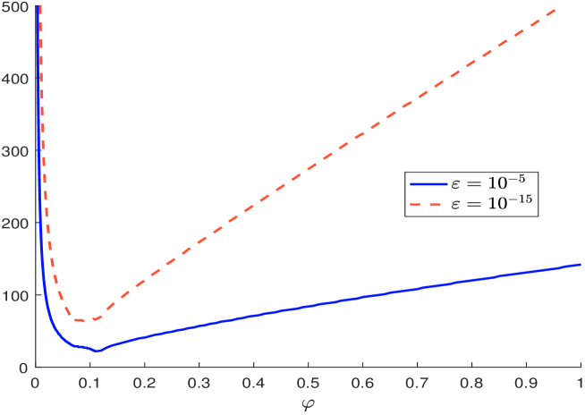
Figure 5: Number of ADMM iterations for finding the ERC portfolio

4.2.2 Risk budgeting optimization

The ERC portfolio has been extended by Roncalli (2013) when the risk budgets are not equal and when the risk measure $\mathcal{R}\left(x\right)$ is convex and coherent:

$$\mathcal{RC}_{i}\left(x\right)=x_{i}\frac{\partial\,\mathcal{R}\left(x\right)}{\partial\,x_{i}}=\mathcal{RB}_{i}$$

where $\mathcal{RB}_{i}$ is the risk budget allocated to Asset $i$. In this case, we can show that the risk budgeting portfolio is the scaled solution of the following optimization problem:

$$x^{\star}=\arg\min_{x}\mathcal{R}\left(x\right)-\lambda\sum_{i=1}^{n}\mathcal{RB}_{i}\cdot\ln x_{i}$$

where $\lambda$ is any positive scalar. Depending on the risk measure, we can use the CCD or the ADMM algorithm.

For example, Roncalli (2015) proposes using the standard deviation-based risk measure:

$$\mathcal{R}\left(x\right)=-x^{\top}\left(\mu-r\right)+\xi\sqrt{x^{\top}\Sigma x}$$

In this case, the first-order condition for defining the CCD algorithm is:

$$-\left(\mu_{i}-r\right)+\xi\frac{\left(\Sigma x\right)_{i}}{\sqrt{x^{\top}\Sigma x}}-\lambda\frac{\mathcal{RB}_{i}}{x_{i}}=0$$

It follows that $\xi x_{i}\left(\Sigma x\right)_{i}-\left(\mu_{i}-r\right)x_{i}\sigma\left(x\right)-\lambda\sigma\left(x\right)\cdot\mathcal{RB}_{i}=0$ or equivalently:

$$\alpha_{i}x_{i}^{2}+\beta_{i}x_{i}+\gamma_{i}=0$$

where $\alpha_{i}=\xi\sigma_{i}^{2}$, $\beta_{i}=\xi\sigma_{i}\sum_{j\neq i}x_{j}\rho_{i,j}\sigma_{j}-\left(\mu_{i}-r\right)\sigma\left(x\right)$ and $\gamma_{i}=-\lambda\sigma\left(x\right)\cdot\mathcal{RB}_{i}$. We notice that the solution $x_{i}$ depends on the volatility $\sigma\left(x\right)$. Here, we face an endogenous problem, because $\sigma\left(x\right)$ depends on $x_{i}$. Griveau-Billon et al. (2015) notice that this is not an issue, because we may assume that $\sigma\left(x\right)$ is almost constant between two coordinate iterations of the CCD algorithm. They deduce that the coordinate solution is then the positive root of the second-degree equation:

$$x_{i}^{\left(k+1\right)}=\frac{-\beta_{i}^{\left(k+1\right)}+\sqrt{\left(\beta_{i}^{\left(k+1\right)}\right)^{2}-4\alpha_{i}^{\left(k+1\right)}\gamma_{i}^{\left(k+1\right)}}}{2\alpha_{i}^{\left(k+1\right)}}$$ (66)

where:

$$\left\{\begin{array}[]{l}\alpha_{i}^{\left(k+1\right)}=\xi\sigma_{i}^{2}\\ \beta_{i}^{\left(k+1\right)}=\xi\sigma_{i}\left(\sum_{j<i}x_{j}^{\left(k+1\right)}\rho_{i,j}\sigma_{j}+\sum_{j>i}x_{j}^{\left(k\right)}\rho_{i,j}\sigma_{j}\right)-\left(\mu_{i}-r\right)\sigma_{i}^{\left(k+1\right)}\left(x\right)\\ \gamma_{i}^{\left(k+1\right)}=-\lambda\sigma_{i}^{\left(k+1\right)}\left(x\right)\cdot\mathcal{RB}_{i}\\ \sigma_{i}^{\left(k+1\right)}\left(x\right)=\sqrt{\chi^{\top}\Sigma\chi}\\ \chi=\left(x_{1}^{\left(k+1\right)},\ldots,x_{i-1}^{\left(k+1\right)},x_{i}^{\left(k\right)},x_{i+1}^{\left(k\right)}\ldots,x_{n}^{\left(k\right)}\right)\end{array}\right.$$

In the case of the volatility or the standard deviation-based risk measure, we apply the exact formulation of the CCD algorithm because we have an analytical solution of the first-order condition. This is not always the case, especially when we consider skewness-based risk measure (Bruder et al., 2016; Lezmi et al., 2018). In this case, we can use the gradient formulation of the CCD algorithm or the ADMM algorithm, which is defined as follows:

$$\left\{\begin{array}[]{l}x^{\left(k+1\right)}=\mathbf{prox}_{\varphi^{-1}\mathcal{R}\left(x\right)}\left(y^{\left(k\right)}-u^{\left(k\right)}\right)\\ v_{y}^{\left(k+1\right)}=x^{\left(k+1\right)}+u^{\left(k\right)}\\ y^{\left(k+1\right)}=\frac{1}{2}\left(v_{y}^{\left(k+1\right)}+\sqrt{v_{y}^{\left(k+1\right)}\odot v_{y}^{\left(k+1\right)}+4\lambda\varphi^{-1}\cdot\mathcal{RB}}\right)\\ u^{\left(k+1\right)}=u^{\left(k\right)}+x^{\left(k+1\right)}-y^{\left(k+1\right)}\end{array}\right.$$

4.2.3 The most diversified portfolio

Choueifaty and Coignard (2008) introduce the concept of diversification ratio, which corresponds to the following expression:

$$\mathcal{DR}\left(x\right)=\frac{\sum_{i=1}^{n}x_{i}\sigma_{i}}{\sigma\left(x\right)}=\frac{x^{\top}\sigma}{\sqrt{x^{\top}\Sigma x}}$$

By construction, the diversification ratio of a portfolio fully invested in one asset is equal to one, whereas it is larger than one in the general case. The authors then propose building the most diversified portfolio as the portfolio which maximizes the diversification ratio. It is also the solution to the following minimization problem:

$$x^{\star} = \arg\min_{x}\frac{1}{2}\ln\left(x^{\top}\Sigma x\right)-\ln\left(x^{\top}\sigma\right)$$

s.t. $$\left\{\begin{array}[]{l}\mathbf{1}_{n}^{\top}x=1\\ x\in\Omega\end{array}\right.$$

This problem is relatively easy to solve using standard numerical algorithms if $\Omega$ corresponds to linear constraints, for example weight constraints. However, the optimal solution may face the same problem as the minimum variance portfolio since most of the time it is concentrated on a small number of assets. This is why it is interesting to add a weight diversification constraint $\mathcal{D}\left(x\right)\geq\mathcal{D}^{-}$. For example, we can assume that the number of effective bets $\mathcal{N}\left(x\right)$ is larger than a minimum acceptable value $\mathcal{N}^{-}$. Contrary to the minimum variance portfolio, we do not obtain a QP problem and we observe that the optimization problem is tricky in practice. Thanks to the ADMM algorithm, we can however simplify the optimization problem by splitting the constraints and using the same approach that has been already described on page 4.1.1. The $x$-update consists in finding the regularized standard MDP:

$$x^{\left(k+1\right)}=\arg\min_{x}\left\{\frac{1}{2}\ln\left(x^{\top}\Sigma x\right)-\ln\left(x^{\top}\sigma\right)+\frac{\varphi}{2}\left\|x-y^{\left(k\right)}+u^{\left(k\right)}\right\|_{2}^{2}\quad\text{s.t. }\mathbf{1}_{n}^{\top}x=1\right\}$$

whereas the $y$-update corresponds to the projection onto the intersection of $\Omega$ and $\mathfrak{D}=\left\{x\in\mathbb{R}^{n}:\mathcal{D}\left(x\right)\geq\mathcal{D}^{-}\right\}$:

$$y^{\left(k+1\right)}=\mathcal{P}_{\Omega\,\cap\,\mathfrak{D}}\left(x^{\left(k+1\right)}+u^{\left(k\right)}\right)$$

We consider the parameter set #2 given in Appendix B on page B. Results are reported in Table 5. The second column corresponds to the long/short MDP portfolio (or $\Omega=\mathbb{R}^{n}$). By definition, we cannot compute the number of effective bets because it contains short positions. The other columns correspond to the long-only MDP portfolio (or $\Omega=\left[0,1\right]^{n}$) when we impose a sufficient number of effective bets $\mathcal{N}^{-}$. We notice that the traditional long-only MDP is poorly diversified in terms of weights since we have $\mathcal{N}\left(x\right)=2.30$. As for the minimum variance portfolio, the MDP tends to the equally-weighted portfolio when $\mathcal{N}^{-}$ tends to the number of assets

Table 5: MDP portfolios (in %)

	L/S	Long-only
$\mathcal{N}^{-}$		$0.00$	$3.00$	$4.00$	$5.00$	$6.00$	$7.00$
$x_{1}^{\star}$	$41.81$	$41.04$	$35.74$	$30.29$	$26.08$	$22.44$	$18.83$
$x_{2}^{\star}$	$51.88$	$50.92$	$43.91$	$36.68$	$31.05$	$26.12$	$21.19$
$x_{3}^{\star}$	$8.20$	$8.05$	$10.12$	$11.52$	$12.33$	$12.80$	$13.01$
$x_{4}^{\star}$	$-0.43$	$0.00$	$2.48$	$5.12$	$7.16$	$8.90$	$10.51$
$x_{5}^{\star}$	$-0.26$	$0.00$	$0.92$	$2.28$	$3.60$	$5.02$	$6.85$
$x_{6}^{\star}$	$-0.38$	$0.00$	$2.03$	$4.36$	$6.28$	$8.02$	$9.79$
$x_{7}^{\star}$	$-0.51$	$0.00$	$3.47$	$6.68$	$8.85$	$10.44$	$11.65$
$x_{8}^{\star}$	$-0.31$	$0.00$	$1.32$	$3.07$	$4.65$	$6.27$	$8.17$
$\mathcal{N}\left(x\right)$		$2.30$	$3.00$	$4.00$	$5.00$	$6.00$	$7.00$

4.3 Robo-advisory optimization

Today’s financial industry is facing a digital revolution in all areas: payment services, on-line banking, asset management, etc. This is particularly true for the financial advisory industry, which has been impacted in the last few years by the emergence of digitalization and robo-advisors. The demand for robo-advisors is strong, which explains the growth of this business. How does one characterize a robo-advisor? This is not simple, but the underlying idea is to build a systematic portfolio allocation in order to provide a customized advisory service. A robo-advisor has two main objectives. The first objective is to know the investor better than a traditional asset manager. Because of this better knowledge, the robo-advisor may propose a more appropriate asset allocation. The second objective is to perform the task in a systematic way and to build an automated rebalancing process. Ultimately, the goal is to offer a customized solution. In fact, the reality is very different. We generally notice that many robo-advisors are more a web or a digital application, but not really a robo-advisor. The reason is that portfolio optimization is a very difficult task. In many robo-advisors, asset allocation is then rather human-based or not completely systematic with the aim to rectify the shortcomings of mean-variance optimization. Over the next five years, the most important challenge for robo-advisors will be to reduce these discretionary decisions and improve the robustness of their systematic asset allocation process. But this means that robo-advisors must give up the quadratic programming world of the portfolio allocation.

4.3.1 Specification of the objective function

In order to make mean-variance optimization more robust, two directions can be followed. The first one has been largely explored and adds a penalty function in order to regularize or sparsify the solution (Brodie et al. 2009; DeMiguel et al., 2009; Carrasco and Noumon, 2010; Bruder et al., 2013; Bourgeron et al., 2018). The second one consists in changing the objective function and considering risk budgeting portfolios instead of mean-variance optimized portfolios (Maillard et al., 2010; Roncalli, 2013). Even if this second direction has encountered great success, it presents a solution that is not sufficiently flexible in terms of active management. Nevertheless, these two directions are not so divergent. Indeed, Roncalli (2013) shows that the risk budgeting optimization can be viewed as a non-linear shrinkage approach of the minimum variance optimization. Richard and Roncalli (2015) propose then a unified approach of smart beta portfolios by considering alternative allocation models as penalty functions of the minimum variance optimization. In particular, they use the logarithmic barrier function in order to regularize minimum variance portfolios. This idea has also been reiterated by de Jong (2018), who considers a mean-variance framework.

Therefore, we propose defining the robo-advisor optimization problem as follows:

$$x_{t+1}^{\star} = \arg\min_{x}f_{\mathcal{R}obo}\left(x\right)$$ (68)

s.t. $$\left\{\begin{array}[]{l}\mathbf{1}_{n}^{\top}x=1\\ \mathbf{0}_{n}\leq x\leq\mathbf{1}_{n}\\ x\in\Omega\end{array}\right.$$ (72)

where:

$$f_{\mathcal{R}obo}\left(x\right) = \frac{1}{2}\left(x-b\right)^{\top}\Sigma_{t}\left(x-b\right)-\gamma\left(x-b\right)^{\top}\mu_{t}+$$ (73)

$$\varrho_{1}\left\|\Gamma_{1}\left(x-x_{t}\right)\right\|_{1}+\frac{1}{2}\varrho_{2}\left\|\Gamma_{2}\left(x-x_{t}\right)\right\|_{2}^{2}+$$

$$\tilde{\varrho}_{1}\left\|\tilde{\Gamma}_{1}\left(x-\tilde{x}\right)\right\|_{1}+\frac{1}{2}\tilde{\varrho}_{2}\left\|\tilde{\Gamma}_{2}\left(x-\tilde{x}\right)\right\|_{2}^{2}-\lambda\sum_{i=1}^{n}\mathcal{RB}_{i}\cdot\ln x_{i}$$

$b$ is the benchmark portfolio, $\tilde{x}$ is the reference portfolio and $x_{t}$ is the current portfolio.

This specification is sufficiently broad that it encompasses most models used by the industry. We notice that the objective function is made up of three parts. The first part corresponds to the MVO objective function with a benchmark. If we set $b$ equal to $\mathbf{0}_{n}$, we obtain the Markowitz utility function. The second part contains $\boldsymbol{\ell}_{1}$- and $\boldsymbol{\ell}_{2}$-norm penalty functions. The regularization can be done with respect to the current allocation $x_{t}$ in order to control the rebalancing process and the smoothness of the dynamic allocation. The regularization can also be done with respect to a reference portfolio, which is generally the strategic asset allocation of the fund. The idea is to control the profile of the fund. For example, if the strategic asset allocation is an 80/20 asset mix policy, we do not want the portfolio to present a defensive or balanced risk profile. Finally, the third part of the objective function corresponds to the logarithmic barrier function, where the parameter $\lambda$ controls the trade-off between MVO optimization and RB optimization. This last part is very important in order to make the dynamic asset allocation more robust. The hyperparameters of the objective function are $\varrho_{1}$, $\varrho_{2}$, $\tilde{\varrho}_{1}$, $\tilde{\varrho}_{2}$ and $\lambda$. They are all positive and can also be set to zero in order to deactivate a penalty function. For instance, $\varrho_{2}$ and $\tilde{\varrho}_{2}$ are equal to zero if we don’t want to have a shrinkage of the covariance matrix $\Sigma_{t}$. The hyperparameters $\varrho_{1}$ and $\tilde{\varrho}_{1}$ can also be equal to zero because the $\boldsymbol{\ell}_{1}$ regularization is generally introduced when specifying the additional constraints $\Omega$. The parameter $\gamma$ is not really a hyperparameter, because it is generally calibrated to target volatility or an expected return. We also notice that this model encompasses the Black-Litterman model thanks to the specification of $\mu_{t}$ (Bourgeron et al., 2018). Another important component of this framework is the specification of the set $x\in\Omega$. It may include traditional constraints such as weight bounds and/or asset class limits, but we can also add non-linear constraints such as a turnover limit, an active share floor or a weight diversification constraint.

4.3.2 Derivation of the general algorithm

Problem (68) is equivalent to solving:

$$x_{t+1}^{\star}=\arg\min_{x}f_{\mathcal{R}obo}^{+}\left(x\right)$$

where the objective function can be broken down as follows:

$$f_{\mathcal{R}obo}^{+}\left(x\right) = f_{\mathrm{MVO}}\left(x\right)+f_{\boldsymbol{\ell}_{1}}\left(x\right)+f_{\boldsymbol{\ell}_{2}}\left(x\right)+f_{\mathrm{RB}}\left(x\right)+$$

$$+\mathbf{\mathds{1}}_{\Omega_{0}}\left(x\right)+\mathbf{\mathds{1}}_{\Omega}\left(x\right)$$

where:

$$f_{\mathrm{MVO}}\left(x\right) = \frac{1}{2}\left(x-b\right)^{\top}\Sigma_{t}\left(x-b\right)-\gamma\left(x-b\right)^{\top}\mu_{t}$$

$$f_{\boldsymbol{\ell}_{1}}\left(x\right) = \varrho_{1}\left\|\Gamma_{1}\left(x-x_{t}\right)\right\|_{1}+\tilde{\varrho}_{1}\left\|\tilde{\Gamma}_{1}\left(x-\tilde{x}\right)\right\|_{1}$$

$$f_{\boldsymbol{\ell}_{2}}\left(x\right) = \frac{1}{2}\varrho_{2}\left\|\Gamma_{2}\left(x-x_{t}\right)\right\|_{2}^{2}+\frac{1}{2}\tilde{\varrho}_{2}\left\|\tilde{\Gamma}_{2}\left(x-\tilde{x}\right)\right\|_{2}^{2}$$

$$f_{\mathrm{RB}}\left(x\right) = -\lambda\sum_{i=1}^{n}\mathcal{RB}_{i}\cdot\ln x_{i}$$

and $\Omega_{0}=\left\{x\in\left[0,1\right]^{n}:\mathbf{1}_{n}^{\top}x=1\right\}$. The ADMM algorithm is implemented as follows:

$$\left\{x^{\star},y^{\star}\right\} = \arg\min f_{x}\left(x\right)+f_{y}\left(y\right)$$

s.t. $$x-y=\mathbf{0}_{n}$$

This is the general approach for solving the robo-advisor problem.

The main task is then to split the function $f_{\mathcal{R}obo}^{+}$ into $f_{x}$ and $f_{y}$. However, in order to be efficient, the $x$- and $y$-update steps of the ADMM algorithm must be easy to compute. Therefore, we impose that the $x$-step is solved using QP or CCD methods while the $y$-step is solved using the Dykstra’s algorithm, where each component corresponds to an analytical proximal operator. Moreover, we also split the set of constraints $\Omega$ into a set of linear constraints $\Omega_{\mathcal{L}inear}$ and a set of non-linear constraints $\Omega_{\mathcal{N}onlinear}$. This lead defining $f_{x}\left(x\right)$ and $f_{y}\left(y\right)$ as follows:

$$\left\{\begin{array}[]{l}f_{x}\left(x\right)=f_{\mathrm{MVO}}\left(x\right)+f_{\boldsymbol{\ell}_{2}}\left(x\right)+\mathbf{\mathds{1}}_{\Omega_{0}}\left(x\right)+\mathbf{\mathds{1}}_{\Omega_{\mathcal{L}inear}}\left(x\right)\\ f_{y}\left(y\right)=f_{\boldsymbol{\ell}_{1}}\left(y\right)+f_{\mathrm{RB}}\left(x\right)+\mathbf{\mathds{1}}_{\Omega_{\mathcal{N}onlinear}}\left(x\right)\end{array}\right.$$ (74)

We notice that $f_{x}\left(x\right)$ has a quadratic form, implying that the $x$-step may be solved using a QP algorithm. Another formulation is:

$$\left\{\begin{array}[]{l}f_{x}\left(x\right)=f_{\mathrm{MVO}}\left(x\right)+f_{\boldsymbol{\ell}_{2}}\left(x\right)+f_{\mathrm{RB}}\left(x\right)\\ f_{y}\left(y\right)=f_{\boldsymbol{\ell}_{1}}\left(y\right)+\mathbf{\mathds{1}}_{\Omega_{0}}\left(x\right)+\mathbf{\mathds{1}}_{\Omega_{\mathcal{L}inear}}\left(x\right)+\mathbf{\mathds{1}}_{\Omega_{\mathcal{N}onlinear}}\left(x\right)\end{array}\right.$$ (75)

In this case, the $x$-step is solved using the CCD algorithm.

4.3.3 Specific algorithms

The ADMM-QP formulation

If we consider Formulation (74), we have:

$$f_{\mathrm{QP}}\left(x\right) = f_{\mathrm{MVO}}\left(x\right)+f_{\boldsymbol{\ell}_{2}}\left(x\right)$$

$$= \frac{1}{2}\left(x-b\right)^{\top}\Sigma_{t}\left(x-b\right)-\gamma\left(x-b\right)^{\top}\mu_{t}+\frac{1}{2}\varrho_{2}\left\|\Gamma_{2}\left(x-x_{t}\right)\right\|_{2}^{2}+\frac{1}{2}\tilde{\varrho}_{2}\left\|\tilde{\Gamma}_{2}\left(x-\tilde{x}\right)\right\|_{2}^{2}$$

$$= \frac{1}{2}x^{\top}Qx-x^{\top}R+C$$

where $Q=\Sigma_{t}+\varrho_{2}\Gamma_{2}^{\top}\Gamma_{2}+\tilde{\varrho}_{2}\tilde{\Gamma}_{2}^{\top}\tilde{\Gamma}_{2}$, $R=\gamma\mu_{t}+\Sigma_{t}b+\varrho_{2}\Gamma_{2}^{\top}\Gamma_{2}x_{t}+\tilde{\varrho}_{2}\tilde{\Gamma}_{2}^{\top}\tilde{\Gamma}_{2}\tilde{x}$ and $C$ is a constant. Using the fourth ADMM trick, we deduce that $x^{\left(k+1\right)}$ is the solution of the following QP problem:

$$x^{\left(k+1\right)} = \arg\min_{x}\frac{1}{2}x^{\top}\left(Q+\varphi I_{n}\right)x-x^{\top}\left(R+\varphi\left(y^{\left(k\right)}-u^{\left(k\right)}\right)\right)$$

s.t. $$\left\{\begin{array}[]{l}\mathbf{1}_{n}^{\top}x=1\\ \mathbf{0}_{n}\leq x\leq\mathbf{1}_{n}\end{array}\right.$$

Since the proximal operators of $f_{\boldsymbol{\ell}_{1}}$ and $f_{\mathrm{RB}}$ have been already computed, finding $y^{\left(k+1\right)}$ is straightforward with the Dykstra’s algorithm as long as the proximal of each non-linear constraint is known.

The ADMM-CCD formulation

If we consider Formulation (75), we have:

$$f_{x}\left(x\right)=f_{\mathrm{QP}}\left(x\right)-\lambda\sum_{i=1}^{n}\mathcal{RB}_{i}\cdot\ln x_{i}$$

Using Appendix A.10 on page A.10, the CCD algorithm applied to $x$-update is:

$$x_{i}^{\left(k+1\right)} = \frac{R_{i}-\sum_{j<i}x_{j}^{\left(k+1\right)}Q_{i,j}-\sum_{j>i}x_{j}^{\left(k\right)}Q_{i,j}}{2Q_{i,i}}+$$

$$\frac{\sqrt{\left(\sum_{j<i}x_{j}^{\left(k+1\right)}Q_{i,j}+\sum_{j>i}x_{j}^{\left(k\right)}Q_{i,j}-R_{i}\right)^{2}+4\lambda_{i}Q_{i,i}}}{2Q_{i,i}}$$

where the matrices $Q$ and $R$ are defined as:

$$Q=\Sigma_{t}+\varrho_{2}\Gamma_{2}^{\top}\Gamma_{2}+\tilde{\varrho}_{2}\tilde{\Gamma}_{2}^{\top}\tilde{\Gamma}_{2}+\varphi I_{n}$$

and:

$$R=\gamma\mu_{t}+\Sigma_{t}b+\varrho_{2}\Gamma_{2}^{\top}\Gamma_{2}x_{t}+\tilde{\varrho}_{2}\tilde{\Gamma}_{2}^{\top}\tilde{\Gamma}_{2}\tilde{x}+\varphi\left(y^{\left(k\right)}-u^{\left(k\right)}\right)$$

and $\lambda_{i}=\lambda\cdot\mathcal{RB}_{i}$. Like the ADMM-QP formulation, the $y$-update step does not pose any particular difficulties.

4.4 Tips and tricks

If we consider the different portfolio optimization approaches presented in Table 1, we have shown how to solve MVO (1), GMV (2), MDP (3), ERC (4) and RB (5) models. The RQE (7) model is equivalent to the GMV (2) model by replacing the covariance matrix $\Sigma$ by the dissimilarity matrix $D$. Below, we implement the Kullback-Leibler model (4) of Bera and Park (2008) using the ADMM framework. Concerning the regularization problems in Table 2, ridge (8), lasso (9) and log-barrier (10) penalty functions have been already covered. Indeed, ridge and lasso penalizations correspond to the proximal operator of $\boldsymbol{\ell}_{1}$- and $\boldsymbol{\ell}_{2}$-norm functions by applying the translation $g\left(x\right)=x-\tilde{x}$. Shannon’s entropy (11) penalization is discussed below. For the constraints that are considered in Table 3, imposing no cash and leverage (12) is done with the proximal of the hyperplane $\mathcal{H}_{yperlane}\left[\mathbf{1}_{n},1\right]$. No short selling (13) and weight bounds (14) are equivalent to considering the box projections $\mathcal{B}_{ox}\left[\mathbf{0}_{n},\infty\right]$ and $\mathcal{B}_{ox}\left[x^{-},x^{+}\right]$. Asset class limits can be implemented using the projection onto the intersection of two half-spaces $\mathcal{H}_{alfspace}\left[\mathbf{1}_{i\in C_{j}},c_{j}^{+}\right]$ and $\mathcal{H}_{alfspace}\left[-\mathbf{1}_{i\in C_{j}},-c_{j}^{-}\right]$. The proximal of the turnover (16) had been already given in Equation (64) on page 64. If we want to impose an upper limit on transaction costs (17), we use the Moreau decomposition and Equation (63). Finally, Section 4.1.1 on page 4.1.1 dealt with the weight diversification problem of the number of active bets. Therefore, it remains to solve leverage limits (18), long/short exposure (19) restrictions and active management constraints: benchmarking (20), tracking error floor (21) and active share floor (22).

4.4.1 Volatility and return targeting

We first consider the $\mu$-problem and the $\sigma$-problem. Targeting a minimum expected return $\mu\left(x\right)\geq\mu^{\star}$ can be implemented in the ADMM framework using the proximal operator of the hyperplane $\mathcal{H}_{yperlane}\left[-\mu,-\mu^{\star}\right]$. In the case of the $\sigma$-problem $\sigma\left(x\right)\leq\sigma^{\star}$, we use the fourth ADMM trick. Let $L$ be the lower Cholesky decomposition of $\Sigma$, we have:

$$\sigma\left(x\right)\leq\sigma^{\star} \Leftrightarrow \sqrt{x^{\top}\Sigma x}\leq\sigma^{\star}$$

$$\Leftrightarrow \sqrt{x^{\top}\left(LL^{\top}\right)x}\leq\sigma^{\star}$$

$$\Leftrightarrow \left\|y^{\top}y\right\|_{2}\leq\sigma^{\star}$$

where $y=L^{\top}x$. It follows that the proximal of the $y$-update is the projection onto the $\boldsymbol{\ell}_{2}$ ball $\mathcal{B}_{2}\left(\mathbf{0}_{n},\sigma^{\star}\right)$.

4.4.2 Leverage management

If we impose a leverage limit $\sum_{i=1}^{n}\left|x_{i}\right|\leq\mathcal{L}^{+}$, we have $\left\|x\right\|_{1}\leq\mathcal{L}^{+}$ and the proximal of the $y$-update is the projection onto the $\boldsymbol{\ell}_{1}$ ball $\mathcal{B}_{1}\left(\mathbf{0}_{n},\mathcal{L}^{+}\right)$. If the leverage constraint concerns the long/short limits $-\mathcal{LS}^{-}\leq\sum_{i=1}^{n}x_{i}\leq\mathcal{LS}^{+}$, we consider the intersection of the two half-spaces $\mathcal{H}_{alfspace}\left[\mathbf{1}_{n},\mathcal{LS}^{+}\right]$ and $\mathcal{H}_{alfspace}\left[-\mathbf{1}_{n},\mathcal{LS}^{-}\right]$. If we consider an absolute leverage $\left|\sum_{i=1}^{n}x_{i}\right|\leq\mathcal{L}^{+}$, we obtain the previous case with $\mathcal{LS}^{-}=\mathcal{LS}^{+}=\mathcal{L}^{+}$. Portfolio managers can also use another constraint concerning the sum of the $k$ largest values:

$$f\left(x\right)=\sum_{i=n-k+1}^{n}x_{\left(i:n\right)}=x_{\left(n:n\right)}+\ldots+x_{\left(n-k+1:n\right)}$$

where $x_{\left(i:n\right)}$ is the order statistics of $x$: $x_{\left(1:n\right)}\leq x_{\left(2:n\right)}\leq\cdots\leq x_{\left(n:n\right)}$. Beck (2017) shows that:

$$\mathbf{prox}_{\lambda f\left(x\right)}\left(v\right)=v-\lambda\mathcal{P}_{\Omega}\left(\frac{v}{\lambda}\right)$$

where:

$$\Omega=\left\{x\in\left[0,1\right]^{n}:\mathbf{1}_{n}^{\top}x=k\right\}=\mathcal{B}_{ox}\left[\mathbf{0}_{n},\mathbf{1}_{n}\right]\cap\mathcal{H}_{yperlane}\left[\mathbf{1}_{n},k\right]$$

4.4.3 Entropy portfolio and diversification measure

Bera and Park (2008) propose using a cross-entropy measure as the objective function:

$$x^{\star} = \arg\min_{x}\mathop{\rm KL}\left(x\mid\tilde{x}\right)$$

s.t. $$\left\{\begin{array}[]{l}\mathbf{1}_{n}^{\top}x=1\\ \mathbf{0}_{n}\leq x\leq\mathbf{1}_{n}\\ \mu\left(x\right)\geq\mu^{\star}\\ \sigma\left(x\right)\leq\sigma^{\star}\end{array}\right.$$

where $\mathop{\rm KL}\left(x\mid\tilde{x}\right)=\sum_{i=1}^{n}x_{i}\ln\left(x_{i}/\tilde{x}_{i}\right)$ and $\tilde{x}$ is a reference portfolio, which is well-diversified (e.g. the EW or ERC portfolio). In Appendix A.8.9 on page A.8.9, we show that the proximal operator of $\lambda\mathop{\rm KL}\left(x\mid\tilde{x}\right)$ is equal to:

$$\mathbf{prox}_{\lambda\mathop{\rm KL}\left(v\mid\tilde{x}\right)}\left(v\right)=\lambda\left(\begin{array}[]{c}W\left(\lambda^{-1}\tilde{x}_{1}e^{\lambda^{-1}v_{1}-\tilde{x}_{1}^{-1}}\right)\\ \vdots\\ W\left(\lambda^{-1}\tilde{x}_{n}e^{\lambda^{-1}v_{n}-\tilde{x}_{n}^{-1}}\right)\end{array}\right)$$

where $W\left(x\right)$ is the Lambert $W$ function.

Remark 9

Using the previous result and the fact that $\mathop{\rm SE}\left(x\right)=-\mathop{\rm KL}\left(x\mid\mathbf{1}_{n}\right)$, we can use Shannon’s entropy to define the diversification measure $\mathcal{D}\left(x\right)=\mathop{\rm SE}\left(x\right)$. Therefore, solving Problem (53) is straightforward when we consider the following diversification set:

$$\mathfrak{D}=\left\{x\in\left[0,1\right]^{n}:-\sum_{i=1}^{n}x_{i}\ln x_{i}\mathbf{\geq}\mathop{\rm SE}\nolimits^{-}\right\}$$

4.4.4 Passive and active management

In the case of the active share, we use the translation property:

$$\mathcal{AS}\left(x\mid\tilde{x}\right) = \frac{1}{2}\sum_{i=1}^{n}\left|x_{i}-\tilde{x}_{i}\right|$$

$$= \frac{1}{2}\left\|x-\tilde{x}\right\|_{1}$$

The proximal operator is given in Appendix A.8.11 on page A.8.11. It is interesting to notice that this type of problem cannot be solved using an augmented QP algorithm since it involves the complement of the $\boldsymbol{\ell}_{1}$ ball and not directly the $\boldsymbol{\ell}_{1}$ ball itself. In this case, we face a maximization problem and not a minimization problem, and the technique of augmented variables does not work.

For tracking error volatility, again we use the fourth ADMM trick:

$$\sigma\left(x\mid\tilde{x}\right) = \sqrt{\left(x-\tilde{x}\right)^{\top}\Sigma\left(x-\tilde{x}\right)}$$

$$= \left\|y\right\|_{2}$$

where $y=L^{\top}x-L^{\top}\tilde{x}$. Using our ADMM notations, we have $Ax+By=c$ where $A=L^{\top}$, $B=-I_{n}$ and $c=L^{\top}\tilde{x}$.

4.4.5 Index sampling

Index sampling is based on the cardinality constraint $\sum_{i=1}^{n}\mathds{1}\left\{x_{i}>0\right\}\leq n_{x}$. It is closed to the $\boldsymbol{\ell}_{0}$-norm function $\left\|x\right\|_{0}=\sum_{i=1}^{n}\mathds{1}\left\{x_{i}\neq 0\right\}$. Beck (2017) derives the proximal of $\lambda\left\|x\right\|_{0}$ on pages 137-138 of his monograph. However, it does not help to solve the index sampling problem, because we are interested in computing the projection onto the $\boldsymbol{\ell}_{0}$ ball and not the proximal of the $\boldsymbol{\ell}_{0}$-norm function. This is why index sampling remains an open problem using the ADMM framework.

5 Conclusion

The aim of this paper is to propose an alternative solution to the quadratic programming algorithm in the context of portfolio allocation. In numerical analysis, the quadratic programming model is a powerful optimization tool, which is computationally very efficient. In portfolio management, the mean-variance optimization model is exactly a quadratic programming model, meaning that it benefits from its computational power. Therefore, the success of the Markowitz allocation model is explained by these two factors: the quadratic utility function and the quadratic programming setup. A lot of academics and professionals have proposed an alternative approach to the MVO framework, but very few of these models are used in practice. The main reason is that these competing models focus on the objective function and not on the numerical implementation. However, we believe that any model which is not tractable will have little success with portfolio managers. The analogy is obvious if we consider the theory of options. The success of the Black-Scholes model lies in the Black-Scholes analytical formula. Over the last thirty years, many models have been created (e.g. local volatility and stochastic volatility models), but only one can really compete with the Black-Scholes model. This is the SABR model, and the main reason is that it has an analytical formula for implied volatility.

This paper focuses then on a general approach for numerically solving non-QP portfolio allocation models. For that, we consider some algorithms that have been successfully applied to machine learning and large-scale optimization. For instance, the coordinate descent algorithm is the fastest method for performing high-dimensional lasso regression, while the Dykstra’s algorithm has been created to find the solution of restricted least squares regression. Since there is a strong link between MVO and linear regression (Scherer, 2007), this is not a surprise if these algorithms can help solve regularized MVO allocation models. However, these two algorithms are not sufficient for defining a general framework. For that, we need to use the alternating direction method of multipliers and proximal gradient methods. Finally, the combination of these four algorithms (CD, ADMM, PO and Dykstra) allows us to consider allocation models that cannot be cast into a QP form.

In this paper, we have first considered allocation models with non-quadratic objective functions. For example, we have used models based on the diversification ratio, Shannon’s entropy or the Kullback-Leibler divergence. Second, we have solved regularized MVO models with non-linear penalty functions such as the $\boldsymbol{\ell}_{p}$-norm penalty or the logarithmic barrier. Third, we have discussed how to handle non-linear constraints. For instance, we have imposed constraints on active share, volatility targeting, leverage limits, transaction costs, etc. Most importantly, these three non-QP extensions can be combined.

With the development of quantitative strategies (smart beta, factor investing, alternative risk premia, systematic strategies, robo-advisors, etc.), the asset management industry has dramatically changed over the last five years. This is just the beginning and we think that alternative data, machine learning methods and artificial intelligence will massively shape investment processes in the future. This paper is an illustration of this trend and shows how machine learning optimization algorithms allow to move away from the traditional QP world of portfolio management.

Appendix

Appendix A Mathematical results

A.1 QP problem when there is a benchmark

Following Roncalli (2013), the excess return $\mathfrak{R}\left(x\mid b\right)$ of Portfolio $x$ with respect to Benchmark $b$ is the difference between the return of the portfolio and the return of the benchmark:

$$\mathfrak{R}\left(x\mid b\right)=\mathfrak{R}\left(x\right)-\mathfrak{R}\left(b\right)=\left(x-b\right)^{\top}\mathfrak{R}$$

It is easy to show that the expected excess return is equal to:

$$\mu\left(x\mid b\right)=\mathbb{E}\left[\mathfrak{R}\left(x\mid b\right)\right]=\left(x-b\right)^{\top}\mu$$

whereas the volatility of the tracking error is given by:

$$\sigma\left(x\mid b\right)=\sigma\left(\mathfrak{R}\left(x\mid b\right)\right)=\sqrt{\left(x-b\right)^{\top}\Sigma\left(x-b\right)}$$

The objective function is then:

$$f\left(x\mid b\right) = \frac{1}{2}\left(x-b\right)^{\top}\Sigma\left(x-b\right)-\gamma\left(x-b\right)^{\top}\mu$$

$$= \frac{1}{2}x^{\top}\Sigma x-x^{\top}\left(\gamma\mu+\Sigma b\right)+\left(\frac{1}{2}b^{\top}\Sigma b+\gamma b^{\top}\mu\right)$$

$$= \frac{1}{2}x^{\top}Qx-x^{\top}R+C$$

where $C$ is a constant which does not depend on Portfolio $x$. We recognize a QP problem where $Q=\Sigma$ and $R=\gamma\mu+\Sigma b$.

A.2 Augmented QP formulation of the turnover management problem

The augmented QP problem is defined by:

$$X^{\star} = \arg\min_{X}\frac{1}{2}X^{\top}QX-X^{\top}R$$

s.t. $$\left\{\begin{array}[]{l}AX=B\\ CX\leq D\\ \mathbf{0}_{3n}\leq X\leq\mathbf{1}_{3n}\end{array}\right.$$

where $X=\left(x_{1},\ldots,x_{n},x_{1}^{-},\ldots,x_{n}^{-},x_{1}^{+},\ldots,x_{n}^{+}\right)$ is a $3n\times 1$ vector, $Q$ is a $3n\times 3n$ matrix:

$$Q=\left(\begin{array}[]{lll}\Sigma&\mathbf{0}_{n\times n}&\mathbf{0}_{n\times n}\\ \mathbf{0}_{n\times n}&\mathbf{0}_{n\times n}&\mathbf{0}_{n\times n}\\ \mathbf{0}_{n\times n}&\mathbf{0}_{n\times n}&\mathbf{0}_{n\times n}\end{array}\right)$$

$R=\left(\gamma\mu,\mathbf{0}_{n},\mathbf{0}_{n}\right)$ is a $3n\times 1$ vector, $A$ is a $\left(n+1\right)\times 3n$ matrix:

$$A=\left(\begin{array}[]{rrr}\mathbf{1}_{n}^{\top}&\mathbf{0}_{n}^{\top}&\mathbf{0}_{n}^{\top}\\ I_{n}&I_{n}&-I_{n}\end{array}\right)$$

$B=\left(1,\bar{x}\right)$ is a $\left(n+1\right)\times 1$ vector, $C=\left(\begin{array}[]{ccc}\mathbf{0}_{n}^{\top}&\mathbf{1}_{n}^{\top}&\mathbf{1}_{n}^{\top}\end{array}\right)$ is a $1\times 3n$ matrix and $D=\boldsymbol{\tau}^{+}$.

A.3 Augmented QP formulation of the MVO problem with transaction costs

The augmented QP problem of dimension $3n$ is defined by:

$$X^{\star} = \arg\min_{X}\frac{1}{2}X^{\top}QX-X^{\top}R$$

s.t. $$\left\{\begin{array}[]{l}AX=B\\ \mathbf{0}_{3n}\leq X\leq\mathbf{1}_{3n}\end{array}\right.$$

where $X=\left(x_{1},\ldots,x_{n},x_{1}^{-},\ldots,x_{n}^{-},x_{1}^{+},\ldots,x_{n}^{+}\right)$ is a $3n\times 1$ vector, $Q$ is a $3n\times 3n$ matrix:

$$Q=\left(\begin{array}[]{lll}\Sigma&\mathbf{0}_{n\times n}&\mathbf{0}_{n\times n}\\ \mathbf{0}_{n\times n}&\mathbf{0}_{n\times n}&\mathbf{0}_{n\times n}\\ \mathbf{0}_{n\times n}&\mathbf{0}_{n\times n}&\mathbf{0}_{n\times n}\end{array}\right)$$

$R=\left(\gamma\mu,-c^{-},-c^{+}\right)$ is a $3n\times 1$ vector, $A$ is a $\left(n+1\right)\times 3n$ matrix:

$$A=\left(\begin{array}[]{rrr}\mathbf{1}_{n}^{\top}&\left(c^{-}\right)^{\top}&\left(c^{+}\right)^{\top}\\ I_{n}&I_{n}&-I_{n}\end{array}\right)$$

and $B=\left(1,\bar{x}\right)$ is a $\left(n+1\right)\times 1$ vector.

A.4 QP problem with a hyperplane constraint

We consider the following QP problem:

$$x^{\star} = \arg\min_{x}\frac{1}{2}x^{\top}Qx-x^{\top}R$$

s.t. $$a^{\top}x=b$$

The associated Lagrange function is:

$$\mathcal{L}\left(x;\lambda\right)=\frac{1}{2}x^{\top}Qx-x^{\top}R+\lambda\left(a^{\top}x-b\right)$$

The first-order conditions are then:

$$\left\{\begin{array}[]{l}\partial_{x}\,\mathcal{L}\left(x;\lambda\right)=Qx-R+\lambda a=\mathbf{0}_{n}\\ \partial_{\lambda}\,\mathcal{L}\left(x;\lambda\right)=a^{\top}x-b=0\end{array}\right.$$

We obtain $x=Q^{-1}\left(R+\lambda a\right)$. Because $a^{\top}x-b=0$, we have $a^{\top}Q^{-1}R+\lambda a^{\top}Q^{-1}a=b$ and:

$$\lambda^{\star}=\frac{b-a^{\top}Q^{-1}R}{a^{\top}Q^{-1}a}$$

The optimal solution is then:

$$x^{\star}=Q^{-1}\left(R+\frac{b-a^{\top}Q^{-1}R}{a^{\top}Q^{-1}a}a\right)$$

A.5 Derivation of the soft-thresholding operator

We consider the following equation:

$$cx-v+\lambda\partial\,\left|x\right|\in 0$$

where $c>0$ and $\lambda>0$. Since we have $\partial\left|x\right|=\mathop{\rm sign}\left(x\right)$, we deduce that:

$$x^{\star}=\left\{\begin{array}[]{ll}c^{-1}\left(v+\lambda\right)&\text{if }x^{\star}<0\\ 0&\text{if }x^{\star}=0\\ c^{-1}\left(v-\lambda\right)&\text{if }x^{\star}>0\end{array}\right.$$

If $x^{\star}<0$ or $x^{\star}>0$, then we have $v+\lambda<0$ or $v-\lambda>0$. This is equivalent to set $\left|v\right|>\lambda>0$. The case $x^{\star}=0$ implies that $\left|v\right|\leq\lambda$. We deduce that:

$$x^{\star}=c^{-1}\cdot\mathcal{S}\left(v;\lambda\right)$$

where $\mathcal{S}\left(v;\lambda\right)$ is the soft-thresholding operator:

$$\mathcal{S}\left(v;\lambda\right) = \left\{\begin{array}[]{ll}0&\text{if }\left|v\right|\leq\lambda\\ v-\lambda\mathop{\rm sign}\left(v\right)&\text{otherwise}\end{array}\right.$$

$$= \mathop{\rm sign}\left(v\right)\cdot\left(\left|v\right|-\lambda\right)_{+}$$

In Figure 6, we have represented the function $\mathcal{S}\left(v;\lambda\right)$ when $\lambda$ is respectively equal to $1$ and $2$.

Remark 10

The soft-thresholding operator is the proximal operator of the $\boldsymbol{\ell}_{1}$-norm $f\left(x\right)=\left\|x\right\|_{1}$. Indeed, we have $\mathbf{prox}_{f}\left(v\right)=\mathcal{S}\left(v;1\right)$ and $\mathbf{prox}_{\lambda f}\left(v\right)=\mathcal{S}\left(v;\lambda\right)$.

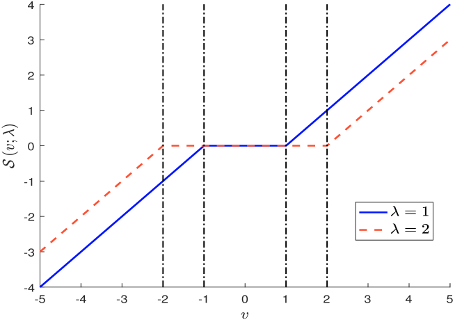
Figure 6: Soft-thresholding operator $\mathcal{S}\left(v;\lambda\right)$

A.6 The box-constrained QP problem

We consider the box-constrained QP problem:

$$x^{\star} = \arg\min_{x}\frac{1}{2}x^{\top}Qx-x^{\top}R$$

s.t. $$x^{-}\leq x\leq x^{+}$$

The objective function is equal to:

$$f\left(x\right) = \frac{1}{2}x^{\top}Qx-x^{\top}R$$

$$= \frac{1}{2}\sum_{i=1}^{n}x_{i}\sum_{j=1}^{n}Q_{i,j}x_{j}-\sum_{i=1}^{n}x_{i}R_{i}$$

$$= \frac{1}{2}\sum_{i=1}^{n}x_{i}\left(Q_{i,i}x_{i}+\sum_{j\neq i}Q_{i,j}x_{j}\right)-\sum_{i=1}^{n}x_{i}R_{i}$$

We deduce that:

$$\frac{\partial\,f\left(x\right)}{\partial\,x_{i}}=\frac{1}{2}\left(2x_{i}Q_{i,i}+\sum_{j\neq i}x_{j}\left(Q_{i,j}+Q_{j,i}\right)\right)-R_{i}$$

We notice that:

$$\frac{\partial\,f\left(x\right)}{\partial\,x_{i}}=0\Leftrightarrow x_{i}=\frac{1}{Q_{i,i}}\left(R_{i}-\sum_{j\neq i}x_{j}\left(\frac{Q_{i,j}+Q_{j,i}}{2}\right)\right)$$

The Lagrange function associated to Problem (A.6) is equal to:

$$\mathcal{L}\left(x;\lambda^{-},\lambda^{+}\right)=f\left(x\right)-\sum_{i=1}^{n}\lambda_{i}^{-}\left(x_{i}-x_{i}^{-}\right)-\sum_{i=1}^{n}\lambda_{i}^{+}\left(x_{i}^{+}-x_{i}\right)$$

The first-order condition is then:

$$\frac{\partial\,\mathcal{L}\left(x;\lambda^{-},\lambda^{+}\right)}{\partial\,x_{i}}=\frac{\partial\,f\left(x\right)}{\partial\,x_{i}}-\lambda_{i}^{-}+\lambda_{i}^{+}=0$$

Since the Kuhn-Tucker conditions are:

$$\left\{\begin{array}[]{c}\min\left(\lambda_{i}^{-},x_{i}-x_{i}^{-}\right)=0\\ \min\left(\lambda_{i}^{+},x_{i}^{+}-x_{i}\right)=0\end{array}\right.$$

we obtain three cases:

1. If no bound is reached, we have $\lambda_{i}^{-}=\lambda_{i}^{+}=0$ and the solution is equal to:

   $$x_{i}^{\star}=\frac{1}{Q_{i,i}}\left(R_{i}-\sum_{j\neq i}x_{j}\left(\frac{Q_{i,j}+Q_{j,i}}{2}\right)\right)$$

2. If the lower bound is reached, we have $\lambda_{i}^{-}>0$, $\lambda_{i}^{+}=0$ and $x_{i}^{\star}=x_{i}^{-}$.

3. If the upper bound is reached, we have $\lambda_{i}^{-}=0$, $\lambda_{i}^{+}>0$ and $x_{i}^{\star}=x_{i}^{+}$.

A.7 ADMM algorithm

The optimization problem is defined as:

$$\left\{x^{\star},y^{\star}\right\} = \arg\min_{\left(x,y\right)}f_{x}\left(x\right)+f_{y}\left(y\right)$$

s.t. $$Ax+By=c$$

The derivation of the algorithm is fully explained in Boyd et al. (2011). For that, they consider the augmented Lagrange function:

$$\mathcal{L}\left(x,y;\lambda,\varphi\right)=f_{x}\left(x\right)+f_{y}\left(y\right)+\lambda^{\top}\left(Ax+By-c\right)+\frac{\varphi}{2}\left\|Ax+By-c\right\|_{2}^{2}$$ (83)

where $\varphi>0$. According to Boyd et al. (2011), the $\boldsymbol{\ell}_{2}$-norm penalty adds robustness to the dual ascent method and accelerates its convergence. The ADMM algorithm uses the property that the objective function is separable, and consists of the following iterations:

$$x^{\left(k+1\right)} = \arg\min_{x}\mathcal{L}\left(x,y^{\left(k\right)};\lambda^{\left(k\right)},\varphi\right)$$

$$= \arg\min_{x}\left\{f_{x}\left(x\right)+\lambda^{\left(k\right)^{\top}}\left(Ax+By^{\left(k\right)}-c\right)+\frac{\varphi}{2}\left\|Ax+By^{\left(k\right)}-c\right\|_{2}^{2}\right\}$$

and:

$$y^{\left(k+1\right)} = \arg\min_{y}\mathcal{L}\left(x^{\left(k+1\right)},y;\lambda^{\left(k\right)},\varphi\right)$$

$$= \arg\min_{y}\left\{f_{y}\left(y\right)+\lambda^{\left(k\right)^{\top}}\left(Ax^{\left(k+1\right)}+By-c\right)+\frac{\varphi}{2}\left\|Ax^{\left(k+1\right)}+By-c\right\|_{2}^{2}\right\}$$

The update for the dual variable $\lambda$ is then:

$$\lambda^{\left(k+1\right)}=\lambda^{\left(k\right)}+\varphi\left(Ax^{\left(k+1\right)}+By^{\left(k+1\right)}-c\right)$$

We repeat the iterations until convergence.

Boyd et al. (2011) notice that the previous algorithm can be simplified. Let $r=Ax+By-c$ be the (primal) residual. By combining linear and quadratic terms, we have:

$$\lambda^{\top}r+\frac{\varphi}{2}\|r\|_{2}^{2}=\frac{\varphi}{2}\left\|r+u\right\|^{2}-\frac{\varphi}{2}\left\|u\right\|^{2}$$

where $u=\varphi^{-1}\lambda$ is the scaled dual variable. We can then write the Lagrange function (83) as follows:

$$\mathcal{L}\left(x,y;u,\varphi\right) = f_{x}\left(x\right)+f_{y}\left(y\right)+\frac{\varphi}{2}\left\|Ax+By-c+u\right\|_{2}^{2}-\frac{\varphi}{2}\left\|u\right\|^{2}$$

$$= f_{x}\left(x\right)+f_{y}\left(y\right)+\frac{\varphi}{2}\left\|Ax+By-c+u\right\|_{2}^{2}-\frac{1}{2\varphi}\left\|\lambda\right\|^{2}$$

Since the last term is a constant, we deduce that the $x$- and $y$-updates become:

$$x^{\left(k+1\right)} = \arg\min_{x}\mathcal{L}\left(x,y^{\left(k\right)};u^{\left(k\right)},\varphi\right)$$ (84)

$$= \arg\min_{x}\left\{f_{x}\left(x\right)+\frac{\varphi}{2}\left\|Ax+By^{\left(k\right)}-c+u^{\left(k\right)}\right\|_{2}^{2}\right\}$$

and:

$$y^{\left(k+1\right)} = \arg\min_{y}\mathcal{L}\left(x^{\left(k+1\right)},y;u^{\left(k\right)},\varphi\right)$$ (85)

$$= \arg\min_{y}\left\{f_{y}\left(y\right)+\frac{\varphi}{2}\left\|Ax^{\left(k+1\right)}+By-c+u^{\left(k\right)}\right\|_{2}^{2}\right\}$$

For the scaled dual variable $u$, we have:

$$u^{\left(k+1\right)} = u^{\left(k\right)}+r^{\left(k+1\right)}$$ (86)

$$= u^{\left(k\right)}+\left(Ax^{\left(k+1\right)}+By^{\left(k+1\right)}-c\right)$$

where $r^{\left(k+1\right)}=Ax^{\left(k+1\right)}+By^{\left(k+1\right)}-c$ is the primal residual at iteration $k+1$. Boyd et al. (2011) also define the variable $s^{\left(k+1\right)}=\varphi A^{\top}B\left(y^{\left(k+1\right)}-y^{\left(k\right)}\right)$ and refer to $s^{\left(k+1\right)}$ as the dual residual at iteration $k+1$.

Under the assumption that the traditional Lagrange function $\mathcal{L}\left(x,y;\lambda,0\right)$ has a saddle point, one can prove that the residual $r^{\left(k\right)}$ converges to zero, the objective function $f_{x}\left(x^{\left(k\right)}\right)+f_{y}\left(y^{\left(k\right)}\right)$ converges to the optimal value $f_{x}\left(x^{\star}\right)+f_{y}\left(y^{\star}\right)$, and the dual variable $\lambda^{\left(k\right)}=\varphi u^{\left(k\right)}$ converges to a dual optimal point. However, the rate of convergence is not known and the primal variables $x^{\left(k\right)}$ and $y^{\left(k\right)}$ do not necessarily converge to the optimal values $x^{\star}$ and $y^{\star}$. In general, the stopping criterion is defined with respect to the residuals:

$$\left\{\begin{array}[]{l}\left\|r^{\left(k+1\right)}\right\|_{2}\leqslant\varepsilon\\[2.84544pt] \left\|s^{\left(k+1\right)}\right\|_{2}\leqslant\varepsilon^{\prime}\end{array}\right.$$

Typical values when implementing this stopping criterion are $\varepsilon=\varepsilon^{\prime}=10^{-15}$ (Bourgeron et al., 2018).

From a theoretical point of view, the convergence holds regardless of the choice of the penalization parameter $\varphi>0$. But the choice of $\varphi$ affects the convergence rate (Ghadimi et al., 2015; Giselsson and Boyd, 2017). In practice, the penalization parameter $\varphi$ may be changed at each iteration, implying that $\varphi$ is replaced by $\varphi^{\left(k\right)}$ and the scaled dual variable $u^{k}$ is equal to $\lambda^{\left(k\right)}/\varphi^{\left(k\right)}$. This may improve the convergence and make the performance independent of the initial choice $\varphi^{\left(0\right)}$. To update $\varphi^{\left(k\right)}$ in practice, He et al. (2000) and Wang and Liao (2001) provide a simple and efficient scheme. On the one hand, the $x$- and $y$-updates in ADMM essentially come from placing a penalty on $\left\|r^{\left(k\right)}\right\|_{2}^{2}$. As a consequence, if $\varphi^{\left(k\right)}$ is large, $\left\|r^{\left(k\right)}\right\|_{2}^{2}$ tends to be small. On the other hand, $s^{\left(k\right)}$ depends linearly on $\varphi$. As a consequence, if $\varphi^{\left(k\right)}$ is small, $\left\|s^{\left(k\right)}\right\|_{2}^{2}$ is small. To keep $\left\|r^{\left(k\right)}\right\|_{2}^{2}$ and $\left\|s^{\left(k\right)}\right\|_{2}^{2}$ within a factor $\mu$, one may consider:

$$\varphi^{\left(k+1\right)}=\left\{\begin{array}[]{ll}\tau\varphi^{\left(k\right)}&\text{if }\left\|r^{\left(k\right)}\right\|_{2}^{2}>\mu\left\|s^{\left(k\right)}\right\|_{2}^{2}\\ \varphi^{\left(k\right)}/\tau^{\prime}&\text{if }\left\|s^{\left(k\right)}\right\|_{2}^{2}>\mu\left\|r^{\left(k\right)}\right\|_{2}^{2}\\ \varphi^{\left(k\right)}&\text{otherwise}\end{array}\right.$$

where $\mu$, $\tau$ and $\tau^{\prime}$ are parameters that are greater than one. In practice, we use $\varphi^{\left(0\right)}=1$, $u^{\left(0\right)}=\mathbf{0}_{p}$, $\mu=10^{3}$ and $\tau=\tau^{\prime}=2$.

Remark 11

The constant case $\varphi^{\left(k+1\right)}=\varphi^{\left(k\right)}=\varphi^{\left(0\right)}$ is obtained by setting $\tau=\tau^{\prime}=1$.

A.8 Proximal operators

A.8.1 Pointwise maximum function

The unit simplex is the generalization of the triangle:

$$\mathbb{S}_{n}=\left\{x\in\left[0,1\right]^{n},\theta_{i}\geq 0:x=\sum_{i=0}^{n}\theta_{i}e_{i},\sum_{i=0}^{n}\theta_{i}=1,\mathbf{1}_{n}^{\top}x\leq 1\right\}$$

where $e_{0}$ is the zero vector and $e_{i}$ are the unit vectors for $i\geq 1$. Beck (2017) shows that $\mathcal{P}_{\mathbb{S}_{n}}\left(v\right)=\left(v-\mu^{\star}\mathbf{1}_{n}\right)_{+}$ where $\mu^{\star}$ is the root of the equation $\mathbf{1}_{n}^{\top}\left(v-\mu^{\star}\mathbf{1}_{n}\right)_{+}=1$. In the case of the pointwise maximum function $f\left(x\right)=\max x$, the Moreau decomposition gives:

$$\mathbf{prox}_{\lambda\max x}\left(v\right) = v-\lambda\mathcal{P}_{\mathbb{S}_{n}}\left(\frac{v}{\lambda}\right)$$

$$= v-\lambda\left(\frac{v}{\lambda}-\mu^{\star}\mathbf{1}_{n}\right)_{+}$$

where $\mu^{\ast}$ is the root of the equation:

$$\mathbf{1}_{n}^{\top}\left(\frac{v}{\lambda}-\mu^{\star}\mathbf{1}_{n}\right)_{+}=1 \Leftrightarrow \sum_{i=1}^{n}\left(\frac{v_{i}}{\lambda}-\mu^{\star}\right)_{+}=1$$

$$\Leftrightarrow \sum_{i=1}^{n}\left(v_{i}-s^{\star}\right)_{+}=\lambda$$

where $s^{\star}=\lambda\mu^{\star}$. It follows that:

$$\mathbf{prox}_{\lambda\max x}\left(v\right) = v-\left(v-s^{\star}\mathbf{1}_{n}\right)_{+}$$

$$= \min\left(v,s^{\star}\right)$$

A.8.2 $\boldsymbol{\ell}_{2}$-norm function

The projection onto the unit ball $\mathcal{B}_{2}\left(\mathbf{0},1\right)=\left\{x\in\mathbb{R}^{n}:\left\|x\right\|_{2}\leq 1\right\}$ is equal to:

$$\mathcal{P}_{\mathcal{B}_{2}\left(\mathbf{0},1\right)}\left(v\right)=\left\{\begin{array}[]{ll}v&\text{if }\left\|v\right\|_{2}\leq 1\\ \dfrac{v}{\left\|v\right\|_{2}}&\text{if }\left\|v\right\|_{2}>1\end{array}\right.$$

Since we have:

$$\mathbf{prox}_{\lambda\left\|x\right\|_{2}}\left(v\right)+\lambda\mathcal{P}_{\mathcal{B}_{2}\left(\mathbf{0},1\right)}\left(\frac{v}{\lambda}\right)=v$$

we deduce that:

$$\mathbf{prox}_{\lambda\left\|x\right\|_{2}}\left(v\right) = v-\lambda\mathcal{P}_{\mathcal{B}_{2}\left(\mathbf{0},1\right)}\left(\frac{v}{\lambda}\right)$$

$$= \left\{\begin{array}[]{ll}v-\lambda\left(\dfrac{v}{\lambda}\right)&\text{if }\left\|v\right\|_{2}\leq\lambda\\[7.11317pt] v-\lambda\dfrac{\dfrac{v}{\lambda}}{\left\|\dfrac{v}{\lambda}\right\|_{2}}&\text{if }\left\|v\right\|_{2}>\lambda\end{array}\right.$$

$$= \left\{\begin{array}[]{ll}0&\text{if }\left\|v\right\|_{2}\leq\lambda\\ v-\dfrac{\lambda v}{\left\|v\right\|_{2}}&\text{if }\left\|v\right\|_{2}>\lambda\end{array}\right.$$

$$= \left(1-\frac{\lambda}{\max\left(\lambda,\left\|v\right\|_{2}\right)}\right)v$$

A.8.3 Scaling and translation

Let $g\left(x\right)=f\left(ax+b\right)$ where $a\neq 0$. Using the change of variable $y=ax+b$, we have:

$$\mathbf{prox}_{g}\left(v\right) = \arg\min_{x}\left\{g\left(x\right)+\frac{1}{2}\left\|x-v\right\|_{2}^{2}\right\}$$

$$= \arg\min_{x}\left\{f\left(ax+b\right)+\frac{1}{2}\left\|x-v\right\|_{2}^{2}\right\}$$

$$= \arg\min_{y}\left\{f\left(y\right)+\frac{1}{2}\left\|\frac{y-b}{a}-v\right\|_{2}^{2}\right\}$$

We deduce that:

$$f\left(y\right)+\frac{1}{2}\left\|\frac{y-b}{a}-v\right\|_{2}^{2} = f\left(y\right)+\frac{1}{2a^{2}}\left\|y-b-av\right\|_{2}^{2}$$

$$= \frac{1}{a^{2}}\left(a^{2}f\left(y\right)+\frac{1}{2}\left\|y-\left(av+b\right)\right\|_{2}^{2}\right)$$

We conclude that $y^{\star}=\mathbf{prox}_{a^{2}f}\left(av+b\right)$ and:

$$\mathbf{prox}_{g}\left(v\right) = \frac{y^{\star}-b}{a}$$

$$= \frac{\mathbf{prox}_{a^{2}f}\left(av+b\right)-b}{a}$$

A.8.4 Projection onto the $\boldsymbol{\ell}_{1}$ ball

We have:

$$x = \mathcal{P}_{\mathcal{B}_{1}\left(c,r\right)}\left(v\right)$$

$$= \mathcal{P}_{\mathcal{B}_{1}\left(\mathbf{0}_{n},r\right)}\left(v-c\right)+c$$

$$= \left(v-c\right)-\mathop{\rm sign}\left(v-c\right)\odot\mathbf{prox}_{r\max x}\left(\left|v-c\right|\right)+c$$

$$= v-\mathop{\rm sign}\left(v-c\right)\odot\min\left(\left|v-c\right|,s^{\star}\right)$$

where $s^{\star}$ is the solution of the following equation:

$$s^{\star}=\left\{s\in\mathbb{R}:\sum_{i=1}^{n}\left(\left|v_{i}-c_{i}\right|-s\right)_{+}=r\right\}$$

Remark 12

$\mathcal{P}_{\mathcal{B}_{1}\left(c,r\right)}\left(v\right)$ is sometimes expressed using the soft-thresholding operator (Beck, 2017, page 151), but the two formulas are equivalent.

A.8.5 Projection onto the $\boldsymbol{\ell}_{2}$ ball

We have:

$$x = \mathcal{P}_{\mathcal{B}_{2}\left(c,r\right)}\left(v\right)$$ (89)

$$= \mathcal{P}_{\mathcal{B}_{2}\left(\mathbf{0}_{n},r\right)}\left(v-c\right)+c$$

$$= \left(v-c\right)-\mathbf{prox}_{r\left\|x\right\|_{2}}\left(v-c\right)+c$$

$$= v-\left(1-\frac{r}{\max\left(r,\left\|v-c\right\|_{2}\right)}\right)\left(v-c\right)$$

$$= c+\frac{r}{\max\left(r,\left\|v-c\right\|_{2}\right)}\left(v-c\right)$$

A.8.6 $\boldsymbol{\ell}_{2}$-penalized logarithmic barrier function

We note $f_{1}\left(x\right)=-\lambda\sum_{i=1}^{n}b_{i}\ln x_{i}$ and $f_{2}\left(x\right)=\mathbf{\mathds{1}}_{\Omega}\left(x\right)$ where $\Omega=\mathcal{B}_{2}\left(c,r\right)$. The Dykstra’s algorithm becomes:

$$\left\{\begin{array}[]{l}v_{x}^{\left(k\right)}=y^{\left(k\right)}+z_{1}^{\left(k\right)}\\ x^{\left(k+1\right)}=\mathbf{prox}_{f_{1}}\left(v_{x}^{\left(k\right)}\right)\\ z_{1}^{\left(k+1\right)}=y^{\left(k\right)}+z_{1}^{\left(k\right)}-x^{\left(k+1\right)}\\ v_{y}^{\left(k\right)}=x^{\left(k+1\right)}+z_{2}^{\left(k\right)}\\ y^{\left(k+1\right)}=\mathbf{prox}_{f_{2}}\left(v_{y}^{\left(k\right)}\right)\\ z_{2}^{\left(k+1\right)}=x^{\left(k+1\right)}+z_{2}^{\left(k\right)}-y^{\left(k+1\right)}\end{array}\right.$$

It follows that:

$$x^{\left(k+1\right)}=\frac{v_{x}^{\left(k\right)}+\sqrt{v_{x}^{\left(k\right)}\odot v_{x}^{\left(k\right)}+4\lambda b}}{2}$$

and:

$$y^{\left(k+1\right)} = \mathcal{P}_{\mathcal{B}_{2}\left(c,r\right)}\left(v_{y}^{\left(k\right)}\right)$$

$$= c+\frac{r}{\max\left(r,\left\|v_{y}^{\left(k\right)}-c\right\|_{2}\right)}\left(v_{y}^{\left(k\right)}-c\right)$$

A.8.7 Quadratic function

Let $f\left(x\right)=\dfrac{1}{2}x^{\top}Qx-x^{\top}R$. We have:

$$\mathbf{prox}_{f}\left(v\right) = \arg\min_{x}\left\{\frac{1}{2}x^{\top}Qx-x^{\top}R+\frac{1}{2}\left\|x-v\right\|_{2}^{2}\right\}$$

$$= \arg\min_{x}\left\{\frac{1}{2}x^{\top}\left(Q+I_{n}\right)x-x^{\top}\left(R+v\right)+\frac{1}{2}v^{\top}v\right\}$$

$$= \left(Q+I_{n}\right)^{-1}\left(R+v\right)$$

A.8.8 Projection onto the intersection of a $\boldsymbol{\ell}_{2}$ ball and a box

We note $f_{1}\left(x\right)=\mathbf{\mathds{1}}_{\Omega_{1}}\left(x\right)$ and $f_{2}\left(x\right)=\mathbf{\mathds{1}}_{\Omega_{2}}\left(x\right)$ where $\Omega_{1}=\mathcal{B}_{2}\left(c,r\right)$ and $\Omega_{2}=\mathcal{B}_{ox}\left[x^{-},x^{+}\right]=\left\{x\in\mathbb{R}^{n}:x^{-}\leq x\leq x^{+}\right\}$. The Dykstra’s algorithm becomes:

$$\left\{\begin{array}[]{l}x^{\left(k+1\right)}=c+\dfrac{r}{\max\left(r,\left\|y^{\left(k\right)}+z_{1}^{\left(k\right)}-c\right\|_{2}\right)}\left(y^{\left(k\right)}+z_{1}^{\left(k\right)}-c\right)\\ z_{1}^{\left(k+1\right)}=y^{\left(k\right)}+z_{1}^{\left(k\right)}-x^{\left(k+1\right)}\\ y^{\left(k+1\right)}=\mathcal{T}\left(x^{\left(k+1\right)}+z_{2}^{\left(k\right)};x^{-},x^{+}\right)\\ z_{2}^{\left(k+1\right)}=x^{\left(k+1\right)}+z_{2}^{\left(k\right)}-y^{\left(k+1\right)}\end{array}\right.$$

This algorithm is denoted by $\mathcal{P}_{\mathcal{B}\mathrm{ox}-\mathcal{B}\mathrm{all}}\left(v;x^{-},x^{+},c,r\right)$.

A.8.9 Shannon’s entropy and Kullback-Leibler divergence

If we consider the scalar function $f\left(x\right)=\lambda x\ln\left(x/\tilde{x}\right)$ where $\tilde{x}$ is a constant, we have:

$$\lambda f\left(x\right)+\frac{1}{2}\left\|x-v\right\|_{2}^{2} = \lambda x\ln\frac{x}{\tilde{x}}+\frac{1}{2}\left(x-v\right)^{2}$$

$$= \lambda x\ln\frac{x}{\tilde{x}}+\frac{1}{2}x^{2}-xv+\frac{1}{2}v^{2}$$

The first-order condition is:

$$\lambda\frac{1}{\tilde{x}}+\lambda\ln\frac{x}{\tilde{x}}+x-v=0 \Leftrightarrow \ln x+\lambda^{-1}x=\ln\tilde{x}+\lambda^{-1}v-\frac{1}{\tilde{x}}$$

$$\Leftrightarrow e^{\ln x+\lambda^{-1}x}=e^{\lambda^{-1}v-\frac{1}{\tilde{x}}+\ln\tilde{x}}$$

$$\Leftrightarrow xe^{\lambda^{-1}x}=\tilde{x}e^{\lambda^{-1}v-\frac{1}{\tilde{x}}}$$

$$\Leftrightarrow \left(\lambda^{-1}x\right)e^{\left(\lambda^{-1}x\right)}=\lambda^{-1}\tilde{x}e^{\lambda^{-1}v-\frac{1}{\tilde{x}}}$$

We deduce that the root is equal to:

$$x^{\star}=\lambda W\left(\frac{\tilde{x}e^{\lambda^{-1}v-\frac{1}{\tilde{x}}}}{\lambda}\right)$$

where $W\left(x\right)$ is the Lambert $W$ function satisfying $W\left(x\right)e^{W\left(x\right)}=x$ (Corless et al., 1996). In the case of the Kullback-Liebler divergence $\mathrm{\mathop{\rm KL}}\left(x\right)=\sum_{i=1}^{n}x_{i}\ln\left(x_{i}/\tilde{x}_{i}\right)$, it follows that:

$$\mathbf{prox}_{\lambda\mathop{\rm KL}\left(v\mid\tilde{x}\right)}\left(v\right)=\lambda\left(\begin{array}[]{c}W\left(\lambda^{-1}\tilde{x}_{1}e^{\lambda^{-1}v_{1}-\tilde{x}_{1}^{-1}}\right)\\ \vdots\\ W\left(\lambda^{-1}\tilde{x}_{n}e^{\lambda^{-1}v_{n}-\tilde{x}_{n}^{-1}}\right)\end{array}\right)$$

Remark 13

The proximal of Shannon’s entropy $\mathrm{\mathop{\rm SE}}\left(x\right)=-\sum_{i=1}^{n}x_{i}\ln x_{i}$ is a special case of the previous result with $\tilde{x}_{i}=1$:

$$\mathbf{prox}_{\lambda\mathop{\rm SE}\left(x\right)}\left(v\right)=\lambda\left(\begin{array}[]{c}W\left(\lambda^{-1}e^{\lambda^{-1}v_{1}-1}\right)\\ \vdots\\ W\left(\lambda^{-1}e^{\lambda^{-1}v_{n}-1}\right)\end{array}\right)$$

This result has been first obtained by Chaux et al. (2007).

A.8.10 Projection onto the complement $\bar{\mathcal{B}}_{2}\left(c,r\right)$ of the $\boldsymbol{\ell}_{2}$ ball

We consider the following proximal problem:

$$x^{\star}=\arg\min_{x}\left\{\mathds{1}_{\Omega}\left(x\right)+\frac{1}{2}\left\|x-v\right\|_{2}^{2}\right\}$$

where:

$$\Omega=\left\{x\in\mathbb{R}^{n}:\left\|x-c\right\|_{2}\geq r\right\}$$

This problem is equivalent to:

$$x^{\star} = \arg\min_{x}\frac{1}{2}\left(x-v\right)^{\top}\left(x-v\right)$$

s.t. $$\left(x-c\right)^{\top}\left(x-c\right)-r^{2}\geq 0$$

We deduce that the Lagrange function is equal to:

$$\mathcal{L}\left(x;\lambda\right)=\frac{1}{2}\left(x-v\right)^{\top}\left(x-v\right)-\lambda\left(\left(x-c\right)^{\top}\left(x-c\right)-r^{2}\right)$$

The first-order condition is:

$$\frac{\partial\,\mathcal{L}\left(x;\lambda\right)}{\partial\,x}=x-v-2\lambda\left(x-c\right)=\mathbf{0}_{n}$$

whereas the KKT condition is $\min\left(\lambda,\left(x-c\right)^{\top}\left(x-c\right)-r^{2}\right)=0$. We distinguish two cases:

1. If $\lambda=0$, this means that $x^{\star}=v$ and $\left(x-c\right)^{\top}\left(x-c\right)-r^{2}>0$.

2. If $\lambda>0$, we have $\left(x-c\right)^{\top}\left(x-c\right)=r^{2}$. Then we obtain the following system:

   $$\left\{\begin{array}[]{l}x-v-2\lambda\left(x-c\right)=\mathbf{0}_{n}\\ \left(x-c\right)^{\top}\left(x-c\right)=r^{2}\end{array}\right.$$

   We deduce that:

   $$\left(x-c\right)-\left(v-c\right)-2\lambda\left(x-c\right)=\mathbf{0}_{n}$$ (90)

   and:

   $$\left(x-c\right)^{\top}\left(x-c\right)-\left(x-c\right)^{\top}\left(v-c\right)-2\lambda\left(x-c\right)^{\top}\left(x-c\right)=0$$

   It follows that $r^{2}-\left(x-c\right)^{\top}\left(v-c\right)-2\lambda r^{2}=0$, meaning that:

   $$\lambda^{\star}=\frac{r^{2}-\left(x-c\right)^{\top}\left(v-c\right)}{2r^{2}}$$

   We notice that:

   $$\left(\ref{eq:proximal-comp-ball1}\right) \Leftrightarrow \left(x-c\right)-\left(v-c\right)-2\frac{r^{2}-\left(x-c\right)^{\top}\left(v-c\right)}{2r^{2}}\left(x-c\right)=\mathbf{0}_{n}$$

   $$\Leftrightarrow -r^{2}\left(v-c\right)+\left(x-c\right)^{\top}\left(v-c\right)\left(x-c\right)=\mathbf{0}_{n}$$

   $$\Leftrightarrow \left(x-c\right)^{\top}\left(v-c\right)\left(x-c\right)=r^{2}\left(v-c\right)$$

   Because $\left(x-c\right)^{\top}\left(v-c\right)$ is a scalar, we deduce that $x-c$ and $v-c$ are two collinear vectors:

   $$x-c=r\frac{\left(v-c\right)}{\left\|v-c\right\|_{2}}$$

   The optimal solution is:

   $$x^{\star}=c+r\frac{\left(v-c\right)}{\left\|v-c\right\|_{2}}$$

Combining the two cases gives:

$$\mathbf{prox}_{\mathds{1}_{\Omega}\left(x\right)}\left(v\right)=c+\frac{r}{\min\left(r,\left\|v-c\right\|_{2}\right)}\left(v-c\right)$$

This is the formula of the projection onto the $\boldsymbol{\ell}_{2}$ ball, but the minimum function has replaced the maximum function.

A.8.11 Projection onto the complement $\bar{\mathcal{B}}_{1}\left(c,r\right)$ of the $\boldsymbol{\ell}_{1}$ ball

This proximal problem associated with $\bar{\mathcal{B}}_{1}\left(\mathbf{0}_{n},r\right)$ is:

$$x^{\star} = \arg\min_{x}\frac{1}{2}\left(x-v\right)^{\top}\left(x-v\right)$$

s.t. $$\left\|x\right\|_{1}\geq r$$

We deduce that the Lagrange function is equal to:

$$\mathcal{L}\left(x;\lambda\right)=\frac{1}{2}\left(x-v\right)^{\top}\left(x-v\right)-\lambda\left(\left\|x\right\|_{1}-r\right)$$

The first-order condition is:

$$\frac{\partial\,\mathcal{L}\left(x;\lambda\right)}{\partial\,x}=x-v-\lambda\mathop{\rm sign}\left(x\right)=\mathbf{0}_{n}$$

whereas the KKT condition is $\min\left(\lambda,\left\|x\right\|_{1}-r\right)=0$. We distinguish two cases:

1. If $\lambda=0$, this means that $x^{\star}=v$ and $\left\|x\right\|_{1}\geq r$.

2. If $\lambda>0$, we have $\left\|x\right\|_{1}=r$. Then we obtain the following system of equations:

   $$\left\{\begin{array}[]{l}x-v=\lambda\mathop{\rm sign}\left(x\right)\\ \left\|x\right\|_{1}=r\end{array}\right.$$

   The first condition gives that $x-v$ is a vector whose elements are $+\lambda$ and/or $-\lambda$, whereas the second condition shows that $x$ is on the surface of the $\boldsymbol{\ell}_{1}$ ball. Unfortunately, there is no unique solution. This is why we assume that $\mathop{\rm sign}\left(x\right)=\mathop{\rm sign}\left(v\right)$ and we modify the sign function: $\mathop{\rm sign}\left(a\right)=1$ if $a\geq 0$ and $\mathop{\rm sign}\left(a\right)=-1$ if $a<0$. In this case, there is a unique solution $x^{\star}=v+\lambda^{\star}\mathop{\rm sign}\left(v\right)$ where $\lambda^{\star}=n^{-1}\left(r-\left\|v\right\|_{1}\right)$ because $\left|v+\lambda\mathop{\rm sign}\left(v\right)\right|=\left|v\right|+\lambda$.

Combining the two cases implies that:

$$\mathcal{P}_{\mathcal{\bar{B}}_{1}\left(\mathbf{0}_{n},r\right)}\left(v\right)=\left\{\begin{array}[]{ll}v&\text{if }\left\|v\right\|_{1}\geq r\\ v+\mathop{\rm sign}\left(v\right)\odot n^{-1}\left(r-\left\|v\right\|_{1}\right)&\text{if }\left\|v\right\|_{1}<r\end{array}\right.$$

Using the translation property, we deduce that:

$$\mathcal{P}_{\mathcal{\bar{B}}_{1}\left(c,r\right)}\left(v\right)=v+\mathop{\rm sign}\left(v-c\right)\odot\frac{\max\left(r-\left\|v-c\right\|_{1},0\right)}{n}$$

A.8.12 The bid-ask linear cost function

If we consider the scalar function:

$$f\left(x\right)=\alpha\left(\gamma-x\right)_{+}+\beta\left(x-\gamma\right)_{+}$$

we have:

$$f_{v}\left(x\right) = \lambda f\left(x\right)+\frac{1}{2}\left\|x-v\right\|_{2}^{2}$$

$$= \lambda\alpha\left(\gamma-x\right)_{+}+\lambda\beta\left(x-\gamma\right)_{+}+\frac{1}{2}x^{2}-xv+\frac{1}{2}v^{2}$$

Following Beck (2017), we distinguish three cases:

1. If $f_{v}\left(x\right)=\lambda\alpha\left(\gamma-x\right)+\frac{1}{2}x^{2}-xv+\frac{1}{2}v^{2}$, then $f_{v}^{\prime}\left(x\right)=-\lambda\alpha+x-v$ and $x^{\star}=v+\lambda\alpha$. This implies that $\gamma-x^{\star}>0$ or $v<\gamma-\lambda\alpha$.

2. If $f_{v}\left(x\right)=\lambda\beta\left(x-\gamma\right)_{+}+\frac{1}{2}x^{2}-xv+\frac{1}{2}v^{2}$, then $f_{v}^{\prime}\left(x\right)=\lambda\beta+x-v$ and $x^{\star}=v-\lambda\beta$. This implies that $x^{\star}-\gamma>0$ or $v<\gamma+\lambda\beta$.

3. If $v\in\left[\gamma-\lambda\alpha,\gamma+\lambda\beta\right]$, the minimum is not obtained at a point of differentiability. Since $\gamma$ is the only point of non-differentiability, we obtain $x^{\star}=\gamma$.

Therefore, we can write the proximal operator in the following compact form:

$$x^{\star}=\gamma+\left(v-\gamma-\lambda\beta\right)_{+}-\left(v-\gamma+\lambda\alpha\right)_{-}$$

where $x_{-}$ and $x_{+}$ are the negative part and the positive part of $x$. If we consider the vector-value function $f\left(x\right)=\sum_{i=1}^{n}\alpha_{i}\left(\gamma_{i}-x_{i}\right)_{+}+\beta_{i}\left(x_{i}-\gamma_{i}\right)_{+}$, we deduce that:

$$\mathbf{prox}_{\lambda f\left(x\right)}\left(v\right)=\gamma+\mathcal{S}\left(v-\gamma;\lambda\alpha,\lambda\beta\right)$$

where $\mathcal{S}\left(v;\lambda_{-},\lambda_{+}\right)=\left(v-\lambda_{+}\right)_{+}-\left(v+\lambda_{-}\right)_{-}$ is the two-sided soft-thresholding operator.

A.9 The QP form of the ADMM-QP problem

We have:

$$f_{\mathrm{QP}}\left(x\right) = f_{\mathrm{MVO}}\left(x\right)+f_{\boldsymbol{\ell}_{2}}\left(x\right)$$

$$= \frac{1}{2}\left(x-b\right)^{\top}\Sigma_{t}\left(x-b\right)-\gamma\left(x-b\right)^{\top}\mu_{t}+\frac{1}{2}\varrho_{2}\left\|\Gamma_{2}\left(x-x_{t}\right)\right\|_{2}^{2}+\frac{1}{2}\tilde{\varrho}_{2}\left\|\tilde{\Gamma}_{2}\left(x-\tilde{x}\right)\right\|_{2}^{2}$$

$$= \frac{1}{2}x^{\top}\Sigma_{t}x-x^{\top}\Sigma_{t}b+\frac{1}{2}b^{\top}\Sigma_{t}b-\gamma x^{\top}\mu_{t}+\gamma b^{\top}\mu_{t}+$$

$$\frac{1}{2}x^{\top}\left(\varrho_{2}\Gamma_{2}^{\top}\Gamma_{2}\right)x-x^{\top}\left(\varrho_{2}\Gamma_{2}^{\top}\Gamma_{2}\right)x_{t}+\frac{1}{2}x_{t}^{\top}\left(\varrho_{2}\Gamma_{2}^{\top}\Gamma_{2}\right)x_{t}+$$

$$\frac{1}{2}x^{\top}\left(\tilde{\varrho}_{2}\tilde{\Gamma}_{2}^{\top}\tilde{\Gamma}_{2}\right)x-x^{\top}\left(\tilde{\varrho}_{2}\tilde{\Gamma}_{2}^{\top}\tilde{\Gamma}_{2}\right)\tilde{x}+\frac{1}{2}\tilde{x}\left(\tilde{\varrho}_{2}\tilde{\Gamma}_{2}^{\top}\tilde{\Gamma}_{2}\right)\tilde{x}$$

$$= \frac{1}{2}x^{\top}\left(\Sigma_{t}+\varrho_{2}\Gamma_{2}^{\top}\Gamma_{2}+\tilde{\varrho}_{2}\tilde{\Gamma}_{2}^{\top}\tilde{\Gamma}_{2}\right)x-x^{\top}\left(\gamma\mu_{t}+\Sigma_{t}b+\varrho_{2}\Gamma_{2}^{\top}\Gamma_{2}x_{t}+\tilde{\varrho}_{2}\tilde{\Gamma}_{2}^{\top}\tilde{\Gamma}_{2}\tilde{x}\right)+$$

$$\gamma b^{\top}\mu_{t}+\frac{1}{2}\left(b^{\top}\Sigma_{t}b+\varrho_{2}x_{t}^{\top}\Gamma_{2}^{\top}\Gamma_{2}x_{t}+\tilde{\varrho}_{2}\tilde{x}\tilde{\varrho}_{2}\tilde{\Gamma}_{2}^{\top}\tilde{\Gamma}_{2}\tilde{x}\right)$$

A.10 The CCD algorithm of a QP form with a logarithmic barrier

We consider the following optimization problem:

$$x^{\star}=\arg\min_{x}\frac{1}{2}x^{\top}Qx-x^{\top}R-\sum_{i=1}^{n}\lambda_{i}\ln x_{i}$$

where $Q$ is a positive-definite matrix and $\lambda_{i}>0$. The first-order condition with respect to coordinate $x_{i}$ is:

$$\left(Qx\right)_{i}-R_{i}-\frac{\lambda_{i}}{x_{i}}=0$$

It follows that $x_{i}\left(Qx\right)_{i}-R_{i}x_{i}-\lambda_{i}=0$ or equivalently:

$$Q_{i,i}x_{i}^{2}+\left(\sum_{j\neq i}x_{j}Q_{i,j}-R_{i}\right)x_{i}-\lambda_{i}=0$$

The polynomial function is convex because we have $Q_{i,i}>0$. Since the product of the roots is negative, we have two solutions with opposite signs. We deduce that the solution is the positive root of the second-degree equation:

$$x_{i}^{\star}=\frac{R_{i}-\sum_{j\neq i}x_{j}Q_{i,j}+\sqrt{\left(\sum_{j\neq i}x_{j}Q_{i,j}-R_{i}\right)^{2}+4\lambda_{i}Q_{i,i}}}{2Q_{i,i}}$$

It follows that CCD algorithm is:

$$x_{i}^{\left(k+1\right)} = \frac{R_{i}-\sum_{j<i}x_{j}^{\left(k+1\right)}Q_{i,j}-\sum_{j>i}x_{j}^{\left(k\right)}Q_{i,j}}{2Q_{i,i}}+$$

$$\frac{\sqrt{\left(\sum_{j<i}x_{j}^{\left(k+1\right)}Q_{i,j}+\sum_{j>i}x_{j}^{\left(k\right)}Q_{i,j}-R_{i}\right)^{2}+4\lambda_{i}Q_{i,i}}}{2Q_{i,i}}$$

Appendix B Data

Parameter set #1

We consider a capitalization-weighted stock index, which is composed of eight stocks. The weights of this benchmark are equal to $23\%$, $19\%$, $17\%$, $9\%$, $8\%$, $6\%$ and $5\%$. We assume that their volatilities are $21\%$, $20\%$, $40\%$, $18\%$, $35\%$, $23\%$, $7\%$ and $29\%$. The correlation matrix is defined as follows:

$$\rho=\left(\begin{array}[]{rrrrrrrr}100\%&&&&&&&\\ 80\%&100\%&&&&&&\\ 70\%&75\%&100\%&&&&&\\ 60\%&65\%&90\%&100\%&&&&\\ 70\%&50\%&70\%&85\%&100\%&&&\\ 50\%&60\%&70\%&80\%&60\%&100\%&&\\ 70\%&50\%&70\%&75\%&80\%&50\%&100\%&\\ 60\%&65\%&70\%&75\%&65\%&70\%&80\%&100\%\end{array}\right)$$

Parameter set #2

We consider a universe of eight stocks. We assume that their volatilities are $25\%$, $20\%$, $15\%$, $18\%$, $30\%$, $20\%$, $15\%$ and $35\%$. The correlation matrix is defined as follows:

$$\rho=\left(\begin{array}[]{rrrrrrrr}100\%&&&&&&&\\ 20\%&100\%&&&&&&\\ 55\%&60\%&100\%&&&&&\\ 60\%&60\%&60\%&100\%&&&&\\ 60\%&60\%&60\%&60\%&100\%&&&\\ 60\%&60\%&60\%&60\%&60\%&100\%&&\\ 60\%&60\%&60\%&60\%&60\%&60\%&100\%&\\ 60\%&60\%&60\%&60\%&60\%&60\%&60\%&100\%\end{array}\right)$$

Appendix C Notations

• $\mu=\left(\mu_{1},\ldots,\mu_{n}\right)$ is the vector of expected return.

• $\Sigma=\left[\rho_{i,j}\sigma_{i}\sigma_{j}\right]_{i,j=1}^{i,j=1}$ is the covariance matrix where $\sigma_{i}$ is the volatility of Asset $i$ and $\rho_{i,j}$ is the correlation between Asset $i$ and Asset $j$.

• $b$ is the vector of benchmark weights.

• $\mu\left(x\right)=x^{\top}\mu$ is the expected return of Portfolio $x$.

• $\sigma\left(x\right)=\sqrt{x^{\top}\Sigma x}$ is the volatility of Portfolio $x$.

• $\mu\left(x\mid b\right)=\left(x-b\right)^{\top}\mu$ is the expected excess return of Portfolio $x$ with respect to Benchmark $b$.

• $\sigma\left(x\mid b\right)=\sqrt{\left(x-b\right)^{\top}\Sigma\left(x-b\right)}$ is the tracking error volatility of Portfolio $x$ with respect to Benchmark $b$.

• $\mathcal{R}\left(x\right)$ is a convex risk measure.

• $\mathcal{RB=}\left(\mathcal{RB}_{1},\ldots,\mathcal{RB}_{n}\right)$ is the vector of risk budgets.

• $\mathcal{RC}_{i}\left(x\right)$ is the risk contribution of Asset $i$ with respect to Portfolio $x$.

• $\boldsymbol{\tau}\left(x\mid\tilde{x}\right)=\sum_{i=1}^{n}\left|x_{i}-\tilde{x}_{i}\right|$ is the turnover between Portfolios $x$ and $\tilde{x}$. The maximum acceptable turnover is denoted by $\boldsymbol{\tau}^{+}$.

• $\boldsymbol{c}\left(x\mid\tilde{x}\right)$ is the cost function when rebalancing Portfolio $x$ from Portfolio $\tilde{x}$. The maximum acceptable cost is denoted by $\boldsymbol{c}^{+}$.

• $\mathcal{AS}\left(x\mid b\right)=\frac{1}{2}\sum_{i=1}^{n}\left|x_{i}-b_{i}\right|$ is the active share of Portfolio $x$ with respect to Benchmark $b$. $\mathcal{AS}^{-}$ is the minimum acceptable active share.

• $\mathcal{H}\left(x\right)=\sum_{i=1}^{n}x_{i}^{2}$ is the Herfindahl index.

• $\mathcal{N}\left(x\right)=1/\mathcal{H}\left(x\right)$ is the number of effective bets. $\mathcal{N}^{-}$ corresponds to the minimum acceptable number of effective bets.

• $\mathcal{DR}\left(x\right)=\left(x^{\top}\sigma\right)/\sqrt{x^{\top}\Sigma x}$ is the diversification ratio of Portfolio $x$.

• $\mathcal{LS}\left(x\right)=\left|\sum_{i=1}^{n}x_{i}\right|$ is the long/short exposure of Portfolio $x$.

• $\mathcal{L}\left(x\right)=\sum_{i=1}^{n}\left|x_{i}\right|$ is the leverage of Portfolio $x$.

• $\mathop{\rm SE}\left(x\right)=-\sum_{i=1}^{n}x_{i}\ln x_{i}$ is Shannon’s entropy of $x$.

• $\mathop{\rm KL}\left(x\right)=\sum_{i=1}^{n}x_{i}\ln\left(x_{i}/\tilde{x}_{i}\right)$ is the Kullback-Leibler divergence between $x$ and $\tilde{x}$.

• $W\left(x\right)$ is the Lambert $W$ function satisfying $W\left(x\right)e^{W\left(x\right)}=x$.

• $\mathbf{0}_{n}$ is the vector of zeros.

• $\mathbf{1}_{n}$ is the vector of ones.

• $e_{i}$ is the unit vector, i.e. $\left[e_{i}\right]_{i}=1$ and $\left[e_{i}\right]_{j}=0$ for all $j\neq i$.

• $x_{-}=\max\left(-x,0\right)=-\min\left(x,0\right)$ is the negative part of $x$.

• $x_{+}=\max\left(x,0\right)$ is the positive part of $x$.

• $\mathds{1}_{\Omega}\left(x\right)$ is the convex indicator function of $\Omega$: $\mathds{1}_{\Omega}\left(x\right)=0$ for $x\in\Omega$ and $\mathds{1}_{\Omega}\left(x\right)=+\infty$ for $x\notin\Omega$.

• $A^{\dagger}$ is the Moore-Penrose pseudo-inverse matrix of $A$.

• $\left\|x\right\|_{p}=\left(\sum_{i=1}^{n}\left|x_{i}\right|^{p}\right)^{1/p}$ is the $\boldsymbol{\ell}_{p}$ norm.

• $\left\|x\right\|_{A}=\left(x^{\top}Ax\right)^{1/2}$ is the weighted $\boldsymbol{\ell}_{2}$ norm.

• $x\odot y$ is the Hadamard element-wise product: $\left[x\odot y\right]_{i,j}=\left[x\right]_{i,j}\left[y\right]_{i,j}$.

• $\mathbf{prox}_{f}\left(v\right)$ is the proximal operator of $f\left(x\right)$: $\mathbf{prox}_{f}\left(v\right)=\arg\min\nolimits_{x}\left\{f\left(x\right)+\frac{1}{2}\left\|x-v\right\|_{2}^{2}\right\}$.

• $\mathcal{S}\left(v;\lambda\right)=\mathop{\rm sign}\left(v\right)\cdot\left(\left|v\right|-\lambda\right)_{+}$ is the soft-thresholding operator.

• $\mathcal{S}\left(v;\lambda_{-},\lambda_{+}\right)=\left(v-\lambda_{+}\right)_{+}-\left(v+\lambda_{-}\right)_{-}$ is the two-sided soft-thresholding operator. We have the following property: $\mathcal{S}\left(v;\lambda\right)=\mathcal{S}\left(v;\lambda,\lambda\right)$.

• $\mathcal{T}\left(v,x^{-},x^{+}\right)=\max\left(x^{-},\min\left(x,x^{+}\right)\right)$ is the truncation operator.

• $\mathcal{P}_{\Omega}\left(v\right)$ is the projection of $v$ onto the set $\Omega$: $\mathcal{P}_{\Omega}\left(v\right)=\arg\min\nolimits_{x\in\Omega}\frac{1}{2}\left\|x-v\right\|_{2}^{2}=\mathbf{prox}_{\mathds{1}_{\Omega}\left(x\right)}\left(v\right)$.

• $\mathbb{S}_{n}$ is the unit simplex with dimension $n$.

• $\mathcal{A}_{ffineset}\left[A,B\right]$ is the affine set $\left\{x\in\mathbb{R}^{n}:Ax=B\right\}$.

• $\mathcal{H}_{yperplane}\left[a,b\right]$ is the hyperplane $\left\{x\in\mathbb{R}^{n}:a^{\top}x=b\right\}$.

• $\mathcal{H}_{alfspace}\left[c,d\right]$ is the half-space $\left\{x\in\mathbb{R}^{n}:c^{\top}x\leq d\right\}$.

• $\mathcal{B}_{ox}\left[x^{-},x^{+}\right]$ is the box $\left\{x\in\mathbb{R}^{n}:x^{-}\leq x\leq x^{+}\right\}$.

• $\mathcal{B}_{p}\left(c,r\right)$ is the $\boldsymbol{\ell}_{p}$-ball $\left\{x\in\mathbb{R}^{n}:\left\|x-c\right\|_{p}\leq r\right\}$.

• $\mathfrak{D}$ is the weight diversification set $\left\{x\in\mathbb{R}^{n}:\mathcal{D}\left(x\right)\geq\mathcal{D}^{-}\right\}$ where $\mathcal{D}\left(x\right)$ is the diversification measure and $\mathcal{D}^{-}$ is the minimum acceptable diversification.

References

- [1] Barankin, E.W., and Dorfman, R. (1956), A Method for Quadratic Programming, Econometrica, 24, pp. 340.
- [2] Barankin, E.W., and Dorfman, R. (1958), On Quadratic Programming, University of California Publications in Statistics, 2(13), pp. 285-318.
- [3] Bauschke, H.H., and Borwein, J.M. (1994), Dykstra’s Alternating Projection Algorithm for Two Sets, Journal of Approximation Theory, 79(3), pp. 418-443.
- [4] Beale, E.M.L. (1959), On Quadratic Programming, Naval Research Logistics Quarterly, 6(3), pp. 227-243.
- [5] Beck, A. (2017), First-Order Methods in Optimization, MOS-SIAM Series on Optimization, 25, SIAM.
- [6] Bera, A.K., and Park, S.Y. (2008), Optimal Portfolio Diversification Using the Maximum Entropy Principle, Econometric Reviews, 27(4-6), pp. 484-512.
- [7] Bishop, C.M. (1995), Neural Networks for Pattern Recognition, Oxford University Press.
- [8] Bourgeron, T., Lezmi, E., and Roncalli, T. (2018), Robust Asset Allocation for Robo-Advisors, arXiv, 1902.05710.
- [9] Brodie, J., Daubechies, I., De Mol, C., Giannone, D., and Loris, I. (2009), Sparse and Stable Markowitz Portfolios, Proceedings of the National Academy of Sciences, 106(30), pp. 12267-12272.
- [10] Bruder, B., Gaussel, N., Richard, J-C., and Roncalli, T. (2013), Regularization of Portfolio Allocation, SSRN, www.ssrn.com/abstract=2767358.
- [11] Bruder, B., Kostyuchyk, N., and Roncalli, T. (2016), Risk Parity Portfolios with Skewness Risk: An Application to Factor Investing and Alternative Risk Premia, SSRN, www.ssrn.com/abstract=2813384.
- [12] Boyd, S., Parikh, N., Chu, E., Peleato, B., and Eckstein, J. (2010), Distributed Optimization and Statistical Learning via the Alternating Direction Method of Multipliers, Foundations and Trends® in Machine learning, 3(1), pp. 1-122.
- [13] Candelon, B., Hurlin, C., and Tokpavi, S. (2012), Sampling Error and Double Shrinkage Estimation of Minimum Variance Portfolios, Journal of Empirical Finance, 19(4), pp. 511-527.
- [14] Carmichael, B., Koumou, G.B., and Moran, K. (2018), Rao’s Quadratic Entropy and Maximum Diversification Indexation, Quantitative Finance, 18(6), pp. 1017-1031.
- [15] Carrasco, M., and Noumon, N. (2010), Optimal Portfolio Selection Using Regularization, University of Montréal, Discussion paper.
- [16] Chaux, C., Combettes, P.L., Pesquet, J.C., and Wajs, V.R. (2007), A Variational Formulation for Frame-based Inverse Problems, Inverse Problems, 23(4), pp. 1495-1518.
- [17] Choueifaty, Y. and Coignard, Y. (2008), Toward Maximum Diversification, Journal of Portfolio Management, 35(1), pp. 40-51.
- [18] Choueifaty, Y., Froidure, T. and Reynier, J. (2013), Properties of the Most Diversified Portflio, Journal of investment strategies, 2(2), pp. 49-70.
- [19] Combettes, P.L., and Müller, C.L. (2018), Perspective Functions: Proximal Calculus and Applications in High-dimensional Statistics, Journal of Mathematical Analysis and Applications, 457(2), pp. 1283-1306.
- [20] Combettes, P.L., and Pesquet, J.C. (2011), Proximal Splitting Methods in Signal Processing, in Bauschke, H.H., Burachik, R.S., Combettes, P.L., Elser, V., Luke, D.R., and Wolkowicz, H. (Eds), Fixed-point Algorithms for Inverse Problems in Science and Engineering, Springer Optimization and Its Applications, 48, pp. 185-212, Springer.
- [21] Corless, R.M., Gonnet, G.H., Hare, D.E., Jeffrey, D.J., and Knuth, D.E. (1996), On the Lambert Function, Advances in Computational Mathematics, 5(1), pp. 329-359.
- [22] Cortes, C., and Vapnik, V. (1995), Support-vector Networks, Machine Learning, 20(3), pp. 273-297.
- [23] Cottle, R.W. and Infanger, G. (2010), Harry Markowitz and the Early History of Quadratic Programming, in Guerard, J.B. (Eds), Handbook of Portfolio Construction, Springer, pp. 179-211.
- [24] Dantzig, G.B. (1961), Quadratic Programming: A Variant of the Wolfe-Markowitz algorithms, Operations Research Center, University of California-Berkeley, Research Report 2.
- [25] de Jong, M. (2018), Portfolio Optimisation in an Uncertain World, Journal of Asset Management, 19(4), pp. 216-221.
- [26] Debreu, G. (1952), Definite and Semidefinite Quadratic Forms, Econometrica, 20(2), pp. 295–300.
- [27] DeMiguel, V., Garlappi, L., Nogales, F.J., and Uppal, R. (2009), A Generalized Approach to Portfolio Optimization: Improving Performance by Constraining Portfolio Norms, Management Science, 55(5), pp. 798-812.
- [28] Douglas, J., and Rachford, H.H. (1956), On the Numerical Solution of Heat Conduction Problems in Two and Three Space Variables, Transactions of the American mathematical Society, 82(2), pp. 421-439.
- [29] Dykstra, R.L. (1983), An Algorithm for Restricted Least Squares Regression, Journal of the American Statistical Association, 78(384), pp. 837-842.
- [30] Frank, M., and Wolfe, P. (1956), An Algorithm for Quadratic Programming, Naval Research Logistics Quarterly, 3, pp. 95-110.
- [31] Friedman, J., Hastie, T., and Tibshirani, R. (2010), Regularization Paths for Generalized Linear Models via Coordinate Descent, Journal of Statistical Software, 33(1), pp. 1-22.
- [32] Gabay, D., and Mercier, B. (1976), A Dual Algorithm for the Solution of Nonlinear Variational Problems via Finite Element Approximation, Computers & Mathematics with Applications, 2(1), pp. 17-40.
- [33] Ghadimi, E., Teixeira, A., Shames, I., and Johansson, M. (2015), Optimal Parameter Selection for the Alternating Direction Method of Multipliers (ADMM): Quadratic Problems, IEEE Transactions on Automatic Control, 60(3), pp. 644-658.
- [34] Giselsson, P., and Boyd, S. (2017), Linear Convergence and Metric Selection for Douglas-Rachford Splitting and ADMM, IEEE Transactions on Automatic Control, 62(2), pp. 532-544.
- [35] Gonzalvez, J., Lezmi, E., Roncalli, T., and Xu, J. (2019), Financial Applications of Gaussian Processes and Bayesian Optimization, arXiv, arxiv.org/abs/1903.04841.
- [36] Gould, N.I.M., and Toint, P.L. (2000), A Quadratic Programming Bibliography, Numerical Analysis Group Internal Report, 1, 142 pages.
- [37] Griveau-Billion, T., Richard, J-C., and Roncalli, T. (2013), A Fast Algorithm for Computing High-dimensional Risk Parity Portfolios, SSRN, www.ssrn.com/abstract=2325255.
- [38] Hastie, T., Tibshirani, R. and Friedman, J. (2009), The Elements of Statistical Learning, Second edition, Springer.
- [39] He, B.S., Yang, H., and Wang, S.L. (2000), Alternating Direction Method with Self-Adaptive Penalty Parameters for Monotone Variational Inequalities, Journal of Optimization Theory and applications, 106(2), pp. 337-356.
- [40] Hildreth, C. (1957), A Quadratic Programming Procedure, Naval Research Logistics Quarterly, 4, pp. 79-85.
- [41] Jacobs, R.A. (1988), Increased Rates of Convergence Through Learning Rate Adaptation, Neural Networks, 1(4), pp. 295-307.
- [42] Jagannathan, R., and Ma, T. (2003), Risk Reduction in Large Portfolios: Why Imposing the Wrong Constraints Helps, Journal of Finance, 58(4), pp. 1651-1684.
- [43] LeCun, Y., Boser, B., Denker, J.S., Henderson, D., Howard, R.E., Hubbard, W., and Jackel, L.D. (1989), Backpropagation Applied to Handwritten Zip Code Recognition, Neural Computation, 1(4), pp. 541-551.
- [44] Lezmi, E., Malongo, H., Roncalli, T., and Sobotka, R. (2018), Portfolio Allocation with Skewness Risk: A Practical Guide, SSRN, www.ssrn.com/abstract=3201319.
- [45] Lindstrom, S.B., and Sims, B. (2018), Survey: Sixty Years of Douglas–Rachford, arXiv, 1809.07181.
- [46] Luo, Z.Q., and Tseng, P. (1992), On the Convergence of the Coordinate Descent Method for Convex Differentiable Minimization, Journal of Optimization Theory and Applications, 72(1), pp. 7-35.
- [47] Luo, Z.Q., and Tseng, P. (1993), Error Bounds and Convergence Analysis of Feasible Descent Methods: A General Approach, Annals of Operations Research, 46(1), pp. 157-178.
- [48] Maillard, S., Roncalli, T. and Teïletche, J. (2010), The Properties of Equally Weighted Risk Contribution Portfolios, Journal of Portfolio Management, 36(4), pp. 60-70.
- [49] Mann, H.B. (1943), Quadratic Forms with Linear Constraints, American Mathematical Monthly, 50, pp. 430-433.
- [50] Markowitz, H. (1952), Portfolio Selection, Journal of Finance, 7(1), pp. 77-91.
- [51] Markowitz, H. (1956), The Optimization of a Quadratic Function Subject to Linear Constraints, Naval Research Logistics Quarterly, 3(1-2), pp. 111-133.
- [52] Martin, A.D. (1955), Mathematical Programming of Portfolio Selections, Management Science, 1(2), pp. 152-166.
- [53] Meucci, A. (2009), Managing Diversification, Risk, 22(5), pp. 74-79.
- [54] Michaud, R.O. (1989), The Markowitz Optimization Enigma: Is ‘Optimized’ Optimal?, Financial Analysts Journal, 45(1), pp. 31-42.
- [55] Nesterov, Y.E. (1983), A Method for Solving the Convex Programming Problem with Convergence Rate , Doklady Akademii Nauk SSSR, 269, pp. 543-547.
- [56] Nesterov, Y. (2004), Introductory Lectures on Convex Optimization: A Basic Course, Applied Optimization, 87, Kluwer Academic Publishers.
- [57] Nesterov, Y. (2012), Efficiency of Coordinate Descent Methods on Huge-scale Optimization Problems, SIAM Journal on Optimization, 22(2), pp. 341-362.
- [58] Parikh, N., and Boyd, S. (2014), Proximal Algorithms, Foundations and Trends® in Optimization, 1(3), pp. 127-239.
- [59] Polyak, B.T. (1964), Some Methods of Speeding Up the Convergence of Iteration Methods, USSR Computational Mathematics and Mathematical Physics, 4(5), pp. 1-17.
- [60] Qian, E. (2005), Risk Parity Portfolios: Efficient Portfolios Through True Diversification, Panagora Asset Management, September.
- [61] Richard, J-C., and Roncalli, T. (2015), Smart Beta: Managing Diversification of Minimum Variance Portfolios, in Jurczenko, E. (Ed.), Risk-based and Factor Investing, ISTE Press – Elsevier.
- [62] Richard, J-C., and Roncalli, T. (2019), Constrained Risk Budgeting Portfolios: Theory, Algorithms, Applications & Puzzles, arXiv, 1902.05710.
- [63] Roncalli, T. (2013), Introduction to Risk Parity and Budgeting, Chapman & Hall/CRC Financial Mathematics Series.
- [64] Roncalli, T. (2015), Introducing Expected Returns into Risk Parity Portfolios: A New Framework for Asset Allocation, Bankers, Markets & Investors, 138, pp. 18-28.
- [65] Scherer, B. (2007), Portfolio Construction & Risk Budgeting, Third edition, Risk Books.
- [66] Tibshirani, R. (1996), Regression Shrinkage and Selection via the Lasso, Journal of the Royal Statistical Society B, 58(1), pp. 267-288.
- [67] Tibshirani, R.J. (2017), Dykstra’s Algorithm, ADMM, and Coordinate Descent: Connections, Insights, and Extensions, in Guyon, I., Luxburg, U.V., Bengio, S., Wallach, H., Fergus, R., Vishwanathan, S., and Garnett, R. (Eds), Advances in Neural Information Processing Systems, 30, pp. 517-528.
- [68] Tseng, P. (1990), Dual Ascent Methods for Problems with Strictly Convex Costs and Linear Constraints: A Unified Approach, SIAM Journal on Control and Optimization, 28(1), pp. 214-242.
- [69] Tseng, P. (2001), Convergence of a Block Coordinate Descent Method for Nondifferentiable Minimization, Journal of Optimization Theory and Applications, 109(3), pp. 475-494.
- [70] Vapnik, V. (1998), Statistical Learning Theory, John Wiley & Sons.
- [71] Wang, S.L., and Liao, L.Z. (2001), Decomposition Method with a Variable Parameter for a Class of Monotone Variational Inequality Problems, Journal of Optimization Theory and Applications, 109(2), pp. 415-429.
- [72] Weston, J.F. and Barenek, W. (1955), Programming Investment Portfolio Construction, Analysts Journal, 11(2), pp. 51-55.
- [73] Wolfe, P. (1959), The Simplex Method for Quadratic Programming, Econometrica, 27(3), pp. 382-398.
- [74] Wright, S.J. (2015), Coordinate Descent Algorithms, Mathematical Programming, 151(1), pp. 3-34
- [75] Yu, J.R., Lee, W.Y., and Chiou, W.J.P. (2014), Diversified Portfolios with Different Entropy Measures, Applied Mathematics and Computation, 241, pp. 47-63.