Manifold Fitting under Unbounded Noise

Abstract

There has been an emerging trend in non-Euclidean statistical analysis of aiming to recover a low dimensional structure, namely a manifold, underlying the high dimensional data. Recovering the manifold requires the noise to be of certain concentration. Existing methods address this problem by constructing an approximated manifold based on the tangent space estimation at each sample point. Although theoretical convergence for these methods is guaranteed, either the samples are noiseless or the noise is bounded. However, if the noise is unbounded, which is a common scenario, the tangent space estimation at the noisy samples will be blurred. Fitting a manifold from the blurred tangent space might increase the inaccuracy. In this paper, we introduce a new manifold-fitting method, by which the output manifold is constructed by directly estimating the tangent spaces at the projected points on the underlying manifold, rather than at the sample points, to decrease the error caused by the noise. Assuming the noise is unbounded, our new method provides theoretical convergence in high probability, in terms of the upper bound of the distance between the estimated and underlying manifold. The smoothness of the estimated manifold is also evaluated by bounding the supremum of twice difference above. Numerical simulations are provided to validate our theoretical findings and demonstrate the advantages of our method over other relevant manifold fitting methods. Finally, our method is applied to real data examples.

Keywords: Manifold learning, Riemannian embedding, Convergence, Smoothness

1 Introduction

Linearity has been viewed as a cornerstone in the development of statistical methodology. For decades, prominent progress in statistics has been made with regard to linearizing the data and the way we analyze them. More recently, various kinds of high-throughput data that share a high dimensional characteristic are often encountered. Although each data point usually represents itself as a long vector or a big matrix, in principle they all can be viewed as points on or near an intrinsic manifold. Moreover, modern data sets no longer comprise samples of real vectors in a real vector space but samples of much more complex structures, taking values in spaces which are naturally not (Euclidean) vector spaces. We are witnessing an explosion in the amount of “complex data” with geometric structure and a growing need for statistical analysis of it utilizing the nature of the data space.

The manifold hypothesis has been carefully studied in Fefferman et al. (2016). Here, we only present several relevant examples to make sense of that hypothesis intuitively: the high dimensional data samples tend to lie near a lower dimensional manifold embedded in the ambient space. The classical Coil20 dataset (Nene et al., 1996), which contains images of 20 objects, may be taken as an example. For each object, images are taken every 5 degrees as the object is rotated on a turntable, and each image is of size $32\times 32$. In this case, the dimension of ambient space is the number of pixels, which is 1024, while the latent intrinsic structure can be compactly described with the angle of rotation. In addition to Coil20, such a structure occurs in many other data collections. In seismology, two-dimensional coordinates of earthquake epicenters are located along a one-dimensional fault line. In face recognition, high-dimensional facial images are controlled by lighting conditions (Georghiades et al., 2001) or head orientations (Happy et al., 2012).

Given such data collection, a natural problem is to fit the manifold from the data collection. Manifold fitting, as opposed to the dimension reduction in manifold learning, seeks to represent the underlying manifold as an embedded sub-manifold of the data space. Once the underlying manifold is learned, many types of analysis can be carried out based on it, such as denoising the observed samples by projecting them to the learned manifold (Gong et al., 2010), generating new data samples from the manifold (Radford et al., 2015), classifying samples according to the manifold (Yao and Zhang, 2019), detecting fault lines for seismological purposes (Yao et al., 2019) etc. This potential makes it significantly worthwhile to formulate the manifold fitting problem, as follows.

Suppose the observed data samples $X=\{x_{i}\in\mathbb{R}^{D}\}_{i=1}^{N}$ are in the form

$$x_{i}=y_{i}+\xi_{i},$$

where $y_{1},\cdots,y_{N}$ are unobserved variables drawn from the uniform distribution supported on the latent manifold ${\cal M}$ with dimension $d<D$. Generally, ${\cal M}$ is assumed to be a compact and smooth sub-manifold embedded in the ambient space $\mathbb{R}^{D}$. The precise conditions on ${\cal M}$ will be given in Section 2.1. The uniform distribution assumption of $y_{i}$ sampled from ${\cal M}$ is the same as those used in the related works (Genovese et al., 2012c, 2014; Mohammed and Narayanan, 2017). Here, $\xi_{1},\cdots\xi_{N}$ are drawn from a distribution $G$. The assumptions about the noisy distribution $G$ differ among the related work. The simplest assumption is that the observed samples are noiseless (Fefferman et al., 2016; Mohammed and Narayanan, 2017). However, some literature assumes that the noise is distributed in a bounded region centered at the origin, which means the observed samples are located in a tube centered at ${\cal M}$ (Genovese et al., 2012a). Other literature, such as Genovese et al. (2012c, 2014); Fefferman et al. (2018), assumes $G$ to be the Gaussian distribution supported on $\mathbb{R}^{D}$, whose density at $\xi$ is

$$(\frac{1}{2\pi\sigma^{2}})^{\frac{D}{2}}\exp(-\frac{\|\xi\|_{2}^{2}}{2\sigma^{2}}).$$ (1.1)

The tail of the Gaussian distribution might make the theoretical analysis more challenging than the previous two cases. Strictly speaking, previous manifold fitting methods have not directly addressed this problem, nor have they shown the convergence of the fitted manifold under this assumption. In this paper, we are concerned with the Gaussian assumption of noisy distribution, and let it be denoted by $G_{\sigma}$ to stress the deviation parameter $\sigma$ hereafter. Under the above settings, the goal of the manifold-fitting problem is to produce a smooth manifold ${\cal M}_{\rm out}$ convergent to ${\cal M}$. Specifically, for any arbitrary $x\in{\cal M}_{\rm out}$, $d(x,{\cal M})\leq O(\sigma)$ holds, provided a sufficiently small $\sigma$. In particular, ${\cal M}_{\rm out}$ gets convergence when $\sigma\to 0$. The latter is the domain where Fefferman et al. (2018) is built on, although they were focused on the sample complexity.

1.1 Related work

Methodological studies for manifold fitting can be traced back to works done a few decades earlier on the principal curve (Hastie and Stuetzle, 1989), with every point on the principal curve/surface defined as the conditional mean value of the points in the orthogonal subspace of the principal curve. Based on Hastie and Stuetzle (1989), many other principal-curve algorithms, like Banfield and Raftery (1992); Stanford and Raftery (2000); Verbeek et al. (2002), have been proposed, attempting to achieve lower estimation bias and better robustness. Recently, Ozertem and Erdogmus (2011) describes the principal curve in a seemingly different way but in a probabilistic sense. In Ozertem and Erdogmus (2011), every point on the principal curve/surface is the local maximum, not the expected value, of the probability density in the local orthogonal subspace. This definition of the principal curve/surface is formulated as a ridge of the probability density. Although it has been demonstrated that these proposed methods give good estimation in many simulated cases, they do not provide theoretical analysis for estimating accuracy, nor the curvature of the output manifold in general cases, with the exception of special cases such as elliptical distributions.

Recently, some works have focused on the theoretical analysis for manifold fitting. In particular, Genovese et al. (2012a) and Genovese et al. (2012c) establish the upper bounds on the Hausdorff distance between the output and underlying manifold under various noise settings, although they do not offer any practical estimators. Genovese et al. (2012b) proposes an estimator which is computationally simple, and whose convergence is guaranteed. However, the conclusions hold only when the noise is supported on a compact set. Genovese et al. (2014) focuses on the ridge of the probability density introduced by Ozertem and Erdogmus (2011), and proposes a convergent algorithm. It is worth noting that the data in Genovese et al. (2014) was assumed to be blurred by homogeneous Gaussian noise, which is more general than the assumption made in Genovese et al. (2012b). Boissonnat and Ghosh (2014) proposed an algoirthm based upon Delauney complexes. The convergence of this algorithm was analyzed by Aamari and Levrard (2018). Aamari and Levrard (2019) presented an algorithm to estimate a point on the manifold, its tangent and second form. Based on these, they approximated the underlying manifold by a mere union of polynomial patches and gave convergence rate for noise-free and tubular noise models. Aizenbud and Sober (2021) presented an algorithm that show convergence to the manifold and its tangent bundle even with tubular noise. However, methods mentioned above are not guaranteed to output an actual $d$-dimensional manifold with certain smoothness.

To overcome this issue, some works about manifold fitting have aimed to determine how curved the output manifold is. In the spirit of Ozertem and Erdogmus (2011) and Genovese et al. (2014), Fefferman et al. (2016) and Mohammed and Narayanan (2017) also took the ridge set into consideration, the former focusing on theoretical analysis and the latter on practical algorithms. Specifically, rather than using the probability density function, they both chose to work with the approximate square-distance functions (asdf), and approximate the underlying manifold by the ridge of the asdf. The theoretical bounds for the manifold fitting have also been considered in Fefferman et al. (2016) and Mohammed and Narayanan (2017), but for only noiseless data; that is, as long as the asdf meets certain regularity conditions, the researchers have shown that the output of the algorithm is a manifold with bounded reach, and the output manifold is arbitrarily close in Hausdorff to the underlying one.

To deal with manifold fitting with noise, Fefferman et al. (2018) proposes a new approach to fit a putative manifold under Gaussian noise. Unlike other methods which use the entire sample set, the method of Fefferman et al. (2018) involves subsampling first such that the number of used samples can be bounded above by $e^{D}$. Under this constraint, the noise is supported on a bounded set with high probability. With this, Fefferman et al. (2018) could carry out their analysis with the bounded noise. However, the constraint on the sample size causes a trouble that the upper bound does not go to zero even if available samples are enough and the variance of Gaussian noise diminishes. Therefore, the methodology is not essentially addressed when the support of noise is unbounded. This potentially leaves room for the manifold-fitting problem, especially from the theoretical side.

1.2 Motivation

In this paper, we attempt to evaluate the convergence and smoothness of ${\cal M}_{\rm out}$. Among the works mentioned previously, Mohammed and Narayanan (2017) and Fefferman et al. (2018) are most relevant to our work. We illustrate these two methods geometrically in Figure 1, where the black curve is a local part of ${\cal M}$, $x$ is a point off ${\cal M}$, and the dots $x_{i}$ and $x_{j}$ represent two samples in the neighborhood of $x$. These two works approximate the underlying manifold by small discs of radius $r$ at every sample points, as the red and blue dashed lines have shown in Figure 1.

For any $x$, Mohammed and Narayanan (2017) define an approximate squared-distance function (asdf) to ${\cal M}$ as the average distance between $x$ and the discs in its neighborhood, which is illustrated as the average length of the red and blue solid lines in the left panel of Figure 1. The output ${\cal M}_{\rm out}$ is then given by the ridge set of the asdf.

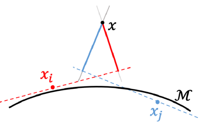
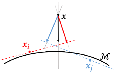
Figure 1: A toy example to illustrate the methodologies in Mohammed and Narayanan (2017) (left panel) and Fefferman et al. (2018) (right panel). Mohammed and Narayanan (2017) focuses on noiseless data. Its key step is to estimate an asdf as the average length of the red and blue solid lines in the left panel, and the output manifold is defined as the ridge of the asdf. Fefferman et al. (2018) deals with noisy data. Its key step is to estimate the bias from $x$ to ${\cal M}$ as the black arrow shown in the right panel, by projecting the average of the red and blue arrow onto the estimated normal space. The output manifold is then defined as points whose biases are zeros.

The method proposed by Fefferman et al. (2018) is illustrated in the right panel of Figure 1. Its key idea is to approximate the bias from $x$ to ${\cal M}$ for any arbitrary $x$ and define the output manifold as points with zero bias. The bias from $x$ to ${\cal M}$ is formulated as the vector $(x^{*}-x)$, where $x^{*}$ is the closest point on ${\cal M}$ to $x$. To obtain the approximation of bias from $x$ to ${\cal M}$, Fefferman et al. (2018) calculate the average bias from $x$ to the discs in its neighborhood, and project the average bias by the estimated orthogonal projection onto the normal space of ${\cal M}$ at $x^{*}$ (the gray solid line).

The effectiveness of both works depend on how well these small discs estimate the original manifold. However, both works require these small discs to pass the sample points, which results in the discs not approximating the manifold well when the sample points deviates from the manifold. When the sample points are blurred by unbounded noise, there would be sample points far away from the original manifold. Hence, under this scenario, the methods proposed by Mohammed and Narayanan (2017) and Fefferman et al. (2018) might face challenging in fitting a manifold.

Even if the sample points are on the manifold, say $x_{i}\in{\cal M}$, the disc at $x_{i}$ fits the local manifold at $x_{i}$ rather than the local manifold at $x^{*}$. The deviation between $x_{i}$ and $x^{*}$ also causes the approximation error of the distance/bias from $x$ to ${\cal M}$. As Figure 1 shows, both the red solid line and the red solid arrow are shorter than the distance/bias from $x$ to ${\cal M}$, and the average between the red and blue one cannot overcome this issue. The above analysis tells us that approximating the distance/bias from $x$ to ${\cal M}$ by the distance/bias from $x$ to nearby discs is inappropriate, which motivates us to invent a new method.

Our basic idea is that a Riemannian manifold can be treated as an affine space locally, and therefore the bias from $x$ to ${\cal M}$ can be equivalently treated as the bias from $x$ to $T_{x^{*}}{\cal M}$. Thus, the key of addressing such a bias is to better estimate $T_{x^{*}}{\cal M}$. To find an affine space, two elements are required: the orthogonal projection $\Pi_{x}$ onto its normal space and one point $\bf{b}$ in this affine space. Under the assumption that a manifold can be approximated well by an affine space locally, samples in the neighborhood of $x$ are located close to $T_{x^{*}}{\cal M}$, with the exception of noise. Therefore, a convex combination of these samples is also located close to $T_{x^{*}}{\cal M}$. Thus, we can estimate $\bf{b}$ using the average of sample points in the neighborhood of $x$. At each sample point, the principal components of its neighbors roughly estimate the tangent space, which means the orthogonal projection operator onto the normal space can be estimated by the orthogonal components of the principal components. And the orthogonal projection $\Pi_{x}$ can be estimated as an average of the estimated orthogonal projection at sample points in its neighborhood. Based on these estimators, we can formulate the affine space using $\{x^{\prime}:\Pi_{x}(x^{\prime}-\bf{b})=\bf{0}\}$.

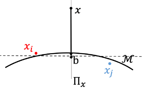
Figure 2: A toy example to illustrate that in our method. $\Pi_{x}$ is used to estimate the orthogonal projection onto the normal space of ${\cal M}$ at $x^{*}$, the black dot $\bf{b}$ is used to estimate a point in $T_{x^{*}}{\cal M}$. Then the space $\{x^{\prime}:\Pi_{x}(x^{\prime}-\bf{b})\}$, illustrated as the black dashed line, approximates $T_{x^{*}}{\cal M}$, and the bias from $x$ to the black dashed line is the estimated bias from $x$ to ${\cal M}$, geometrically illustrated as the black arrow.

The advantages of our method are twofold. On the one hand, we directly approximate the local manifold at $x^{*}$, while existing works approximate the local manifold near the sample points, such as $x_{i}$. On the other hand, we approximate the manifold using a space passing $\bf{b}$ instead of any sample point. Benefit from the mutual offset of noise, $\bf{b}$ hardly deviated far away from $T_{x^{*}}{\cal M}$ even if the noise is unbounded. As a result, we can expect $\{x^{\prime}:\Pi_{x}(x^{\prime}-\bf{b})\}$ to be a better approximation to the local manifold at $x^{*}$, which guarantees the bias from $x$ to $\{x^{\prime}:\Pi_{x}(x^{\prime}-\bf{b})\}$ is a better approximation to the bias from $x$ to ${\cal M}$. The toy example in Figure 2 illustrates the superiority of our method. The black arrow in Figure 2 is almost the bias from $x$ to ${\cal M}$, while both the average length of the solid lines in the left panel of Figure 1 and the black arrow in the right panel of Figure 1 is shorter than the ideal one.

1.3 Main contribution

From a statistical viewpoint, the development of a practical estimator with theoretical bounds satisfying the following requirements simultaneously is urgently required, which improves beyond the requirements by Fefferman et al. (2018):

• The support of noise is unbounded.

• The estimator shares similar geometric property of ${\cal M}$.

• For any arbitrary $x\in{\cal M}_{\rm out}$, the distance between $x$ and ${\cal M}$ is bounded above provided $N$ is sufficiently large and $\sigma$ is sufficiently small. In particular, the distance goes to zero as noise disappears.

• The smoothness of ${\cal M}_{\rm out}$ is mathematically guaranteed.

In this paper, we propose a novel approximation $f(x)$ to the bias from any point $x$ to ${\cal M}$ and fit the underlying manifold ${\cal M}$ in the ambient space as the points with $f(x)=\bf{0}$. Practically, such an output manifold can be achieved by solving the minimization $\|f(x)\|_{2}^{2}$ via gradient descent. This paper provides two main contributions, the first being the theoretical analysis satisfying the above four requirements as follows:

• The noise is assumed to be drawn from the Gaussian distribution $G_{\sigma}$ defined in (1.1).

• Any abitrary neighborhood of ${\cal M}_{\rm out}$ is a $d$-dimensional manifold.

• For any $x\in{\cal M}_{\rm out}$, $d(x,{\cal M})\leq O(\sigma)$ given a large-enough dataset. Thus, ${\cal M}_{\rm out}$ converges to ${\cal M}$ for an increasingly large sample size and diminishing noise.

• The twice difference of ${\cal M}_{\rm out}$ is bounded above by $O(\frac{1}{\sqrt{\sigma}})$.

The second important contribution of this paper is the performance of our estimator in practice. As illustrated in Figures 1 and 2, the bias from a point $x$ to ${\cal M}$ is approximated better than by the other two relevant methods. Numeric results in Section 5 demonstrate the improved performance, which further suggests that our method outputs the approximated manifold to the underlying one.

1.4 Dimension reduction

In addition to manifold fitting, dimension reduction is another important branch in manifold learning. For completeness, this section provides a brief review of this branch.

For the past two decades, there have been a series of dimension reduction methods that try to explore the intrinsic structure of the data by finding its lower-dimensional embedding. These methods, which are usually referred to collectively as manifold learning, are mostly focused on mapping the data from the ambient space to a low-dimensional one. There are generally two kinds of dimension reduction, linear or nonlinear, depending on whether the underlying manifold is assumed to be linear or nonlinear. Of all these methods, the most used one that reduces the dimension of feature space is PCA. To address features lying in a non-linear space (i.e., manifold), methods such as Local Linear Embedding (LLE) (Roweis and Saul, 2000), Isomap (Tenenbaum et al., 2000), MDS Cox and Cox (2000), Laplacian eigenmaps (Belkin and Niyogi, 2003), and LTSA (Zhang and Zha, 2004) are preferred. These non-linear dimension reduction methods rely on spectral graph theory and find the low-dimensional embedding by preserving the local properties of the data. A comprehensive review is provided by Ma and Fu (2011).

Unlike manifold fitting, the outputs of most, if not all, dimension reduction methods are low-dimensional embeddings rather than the points in the ambient space. For the applications listed at the beginning of this paper, such as denoising and data generation, pure low-dimensional embeddings are not enough. This makes manifold fitting quite an open and important problem.

1.5 Organization

The rest of the paper is organized as follows. In Section 2 our approximation ${\cal M}_{\rm out}$ to the underlying manifold ${\cal M}$ is formulated. After that, the convergence and smoothness of ${\cal M}_{\rm out}$ is analyzed in Theorem 5 and Theorem 7 respectively. Section 3 studies the function $f$ defined in (2.5) and determines the properties of its kernel space, the first and second derivatives. Based on these properties of $f$, the proofs of Theorem 5 and Theorem 7 are derived in Section 4. Section 5 contains all numeric examples.

2 Proposed method

2.1 Content and notations

Throughout this paper, the underlying manifold is denoted as ${\cal M}$ and our approximation to ${\cal M}$ is denoted as ${\cal M}_{\rm out}$. For a set $A\subset\mathbb{R}^{D}$ and a point $x\in\mathbb{R}^{D}$, $\Pi_{A}x$ denotes the projection of $x$ onto $A$, namely the nearest point in $A$ to $x$. So $\Pi_{{\cal M}}x$ is the projection of $x$ onto the underlying manifold. If there is no ambiguity, we might use $x^{*}$ instead of $\Pi_{\cal M}x$ for simplicity. The distance between $x$ and $A$, denoted by $d(x,A)$, is the Euclidean distance between $\Pi_{A}x$ and $x$. For any $x^{*}\in{\cal M}$, $T_{x^{*}}{\cal M}$ denotes the tangent space of ${\cal M}$ at $x^{*}$ and $\Pi_{x^{*}}^{*}$ denotes the orthogonal projection onto the normal space of ${\cal M}$ at $x^{*}$. We will make frequent use of the lower-cases $c,c_{0},c_{1},$ etc. and upper-cases $C,C_{0},C_{1}$ etc., in the rest of this paper. The lower-cases and upper-cases denote generic constants less or greater than $1$, whose values may change from line to line. By constants, we mean they are independent of the radius $r$, the standard deviation $\sigma$ or $x$.

We denote $B_{D}(x,r)$ as the Euclidean ball in $\mathbb{R}^{D}$ centered at $x$ of radius $r$, which defines a neighborhood of $x$. The index set $I_{x,r}$ is defined as the indices of the sample points in $B_{D}(x,r)$, and $|I_{x,r}|$ denotes the cardinality of $I_{x,r}$. As given in (1.1), $\sigma$ represents the standard deviation of noise. Throughout this paper, we assume

$$r=O(\sqrt{\sigma}),\quad\sigma<1$$ (2.1)

without loss of generality, otherwise the data could be rescaled so that $\sigma<1$ holds. The underlying manifold ${\cal M}$ is supposed to be boundaryless, compact, $d$-dimensional, and twice differentiable, with a reach bounded by $\tau>0$. The concept reach is a measure of the regularity of the manifold, first introduced by Federer (Federer, 1959) as follows:

Definition 1 (Reach).

Let ${\cal M}$ be a closed subset of $\mathbb{R}^{D}$. The reach of ${\cal M}$, denoted by ${\rm reach}({\cal M})$, is the largest number $\tau$ to have the property that any point at a distance $r<\tau$ from ${\cal M}$ has a unique nearest point in ${\cal M}$.

An important understanding of reach is that it is a twice differential quantity if the manifold is treated as a function. Specifically, if $\gamma$ is an arc-length parametrized geodesic of ${\cal M}$, then for all $t$, $\|\gamma^{\prime\prime}(t)\|\leq 1/\tau$ according to Niyogi et al. (2008). As a twice differential quantity, it is easy to understand that the reach describes how flat the manifold is locally. For example, the reach of a sharp cusp is zero, and the reach of a linear subspace is infinite. Thus, it is natural that the reach measures how close a manifold is to the tangent space locally. The following proposition by Federer (1959) explains this phenomenon:

Proposition 2.

$${\rm reach}({\cal M})^{-1}=\sup\bigg{\{}\frac{2d(y,T_{x}{\cal M})}{\|x-y\|_{2}^{2}}|x,y\in{\cal M},x\neq y\bigg{\}}$$ (2.2)

We emphasize that if ${\rm reach}({\cal M})>0$, the error between ${\cal M}$ and $T_{x}{\cal M}$ at $y$ is of a higher order than $\|x-y\|_{2}$. Thus, in a small-enough neighbor of $x$, we can estimate ${\cal M}$ by $T_{x}{\cal M}$ with negligible error. This is the foundation of our approximation.

The approximation ${\cal M}_{\rm out}$ is defined using the noisy sample points $\{x_{i}\}_{i=1}^{N}$. The number of sample points should be sufficiently large such that $B_{D}(x,r)$ contains enough sample points. Proposition 3 claims the relationship between $|I_{x,r}|$ and $N$.

Proposition 3.

Suppose $x$ satisfies $d(x,{\cal M})\leq cr$ with some $c<1$. There exists constants $c^{\prime}$ and $C$ such that $|I_{x,r}|\geq c^{\prime}r^{d}N$ in probability at least $1-C/\sqrt{N}$.

Proof of proposition 3 is given in Appendix A.1. Based on this proposition, the requirement on $|I_{x,r}|$ can be transformed to the requirement on $N$ for further analysis in later sections. Specifically, $N$ is required to be a sufficiently large quantity in the order of $O(r^{-(d+2)})$.

2.2 Definition of the approximated manifold

Recalling the introduction in Section 1, the definition of ${\cal M}_{\rm out}$ requires to first approximate $T_{x^{*}}{\cal M}$ by $\{x^{\prime}:\Pi_{x}(x^{\prime}-\bf{b})\}$, so that the bias $f(x)$ from $x$ to ${\cal M}$ can be approximated by the bias from $x$ to $\{x^{\prime}:\Pi_{x}(x^{\prime}-\bf{b})\}$, and finally the approximated manifold is defined as the points with $f(x)=\bf{0}$. Now, we formulate the variables and function above.

In order to approximates the orthogonal projection onto the normal space of ${\cal M}$ at $x^{*}$, $\Pi_{x}$ is defined as the weighted average of $\{P_{x_{i}}\}_{i\in I_{x,r}}$, where $P_{x_{i}}$ is the orthogonal projection perpendicular to the first $d$ principal components in $B_{D}(x_{i},r^{\prime})$. Mathematically, $P_{x_{i}}=V_{\bot}V_{\bot}^{T}$, where $V_{\bot}$ is the orthogonal component of $V$ and $V$ is the $D\times d$ matrix whose columns are the eigenvectors corresponding to the largest $d$ eigenvalues of $\sum_{j\in I_{x_{i},r^{\prime}}}(x_{j}-x_{i})(x_{j}-x_{i})^{T}$. The radius $r^{\prime}$ should be sufficiently large, so that the intersection of $B_{D}(x_{i},r^{\prime})$ and ${\cal M}$ is nonempty. Further analysis in Section 3.1 explains that we need $r^{\prime}\geq 2r$.

As the weighted average of $\{P_{x_{i}}\}_{i\in I_{x,r}}$,

$$\Pi_{x}=\Pi_{\rm hi}(A_{x}),\quad A_{x}=\sum_{i\in I_{x,r}}\alpha_{i}(x)P_{x_{i}}.$$ (2.3)

Here, $\Pi_{\rm hi}(A)$ denotes the projection onto the span of the eigenvectors corresponding to the largest $D-d$ eigenvalues of $A$. Specifically, $\Pi_{\rm hi}\big{(}A\big{)}=VV^{T}$, $V$ is a $D\times(D-d)$ matrix whose columns are the eigenvectors corresponding to the largest $D-d$ eigenvalues of $A$. And the weights $\alpha_{i}:\mathbb{R}^{D}\to\mathbb{R}$ in (2.3) are defined as follows:

$$\tilde{\alpha}_{i}(x)=\begin{cases}\left(1-\frac{\|x-x_{i}\|_{2}^{2}}{r^{2}}\right)^{\beta},&x\in B_{D}(x_{i},r)\\ 0,&{\mbox{o}therwise}\end{cases},\quad\tilde{\alpha}(x)=\sum_{i}\tilde{\alpha}_{i}(x),\quad\alpha_{i}(x)=\frac{\tilde{\alpha}_{i}(x)}{\tilde{\alpha}(x)},$$ (2.4)

with $\beta\geq 2$ a fixed integer guaranteeing $f(x)$ in (2.5) to be twice differentiable.

Recalling the weights in (2.4), we formulate $\bf{b}=\sum_{i\in I_{x,r}}\alpha_{i}(x)x_{i}$ as the average of sample points in the neighborhood of $x$. Then the bias from $x$ to the space $\{x^{\prime}:\Pi_{x}(x^{\prime}-\bf{b})\}$ is

$$f(x):\mathbb{R}^{D}\to\mathbb{R}^{D},\quad f(x)=\Pi_{x}\bigg{(}x-\sum_{i\in I_{x,r}}\alpha_{i}(x)x_{i}\bigg{)}.$$ (2.5)

Finally, we give the definition of the approximation as

$${\cal M}_{\rm out}=\{x:d(x,{\cal M})\leq cr,\ f(x)={\bf 0},c<1\},$$ (2.6)

that is, the points with zero bias. By Definition 11 of Fefferman et al. (2016), $\tilde{{\cal M}}=\{x:d(x,{\cal M})\leq cr\}$ is a manifold. Restrict $f$ to $\tilde{{\cal M}}$. When ${\bf 0}$ is regular, the preimage $f^{-1}({\bf 0})={\cal M}_{\rm out}\subset\tilde{{\cal M}}$ is a smooth submanifold. So we call ${\cal M}_{\rm out}$ as the approximated manifold in the paper. Further characterization of the approximated manifold will be discussed in Theorem 4.

The definition of ${\cal M}_{\rm out}$ is practical. Theorem 5 in the next section claims that ${\cal M}_{\rm out}$ approximates ${\cal M}$ in the order of $O(r^{2})$. This means if we have an initial estimator of ${\cal M}$ with error $cr$, then we could achieve a better estimator of ${\cal M}$ using the definition of ${\cal M}_{\rm out}$. In practice, we solve the minimization $\|f(x)\|_{2}^{2}$ via the gradient descent method given the initial estimator, and the output of the gradient descent method approximates ${\cal M}$ in the order of $O(r^{2})$, better than the initial guess.

2.3 Convergence and smoothness of the approximated manifold

In Theorem 4, we prove any arbitrary neighborhood of ${\cal M}_{\rm out}$ is a $d$-dimensional manifold in high probability. In Theorem 5, we characterize the convergence of ${\cal M}_{\rm out}$ in the probability $\delta_{0}(1-\delta)^{2}$, where we denote $\delta_{0}=1-d\exp\{\frac{-c{r}^{d+2}N}{2\ln 2}\}$ for convenience. When $N$ is sufficiently large as we set, $\delta_{0}$ is a high probability. Theorem 5 tells us that if $r=O(\sqrt{\sigma})$ is sufficiently small, ${\cal M}_{\rm out}$ is a good estimator to ${\cal M}$. Moreover, Corollary 6 tells us that the approximated manifold ${\cal M}_{\rm out}$ converges to the underlying manifold ${\cal M}$ as $\sigma\to 0$.

Theorem 4.

Given $\delta>0$ and any arbitrary $x\in{\cal M}_{\rm out}$, there exists $\epsilon$ such that ${\cal M}_{\rm out}\cap B_{D}(x,\epsilon)$ is a $d$-dimensional manifold in probability $\delta_{0}(1-\delta)^{2}\big{(}1-(1-cr^{d})^{N}\big{)}$.

Theorem 5.

Given $\delta>0$, there exists a constant $C$ such that $d(x,{\cal M})\leq Cr^{2}$ for any arbitrary $x\in{\cal M}_{\rm out}$ in probability at least $\delta_{0}(1-\delta)^{2}$.

We point that Theorem 5 holds assuming $\sigma<1$ and $r=O(\sqrt{\sigma})$ as (2.1) claims. If we further assume $\sigma\to 0$, we achieve the following corollary:

Corollary 6.

For any arbitrary $x\in{\cal M}_{\rm out}$, $d(x,{\cal M})\to 0$ as $\sigma\to 0$ in probability at least $\delta_{0}(1-\delta)^{2}$.

Proof  Given $r=O(\sqrt{\sigma})$, there exists $C_{0}$ such that $r=C_{0}\sqrt{\sigma}$. For any $\epsilon>0$, let $\sigma=\frac{\epsilon}{CC_{0}^{2}}$, and then $d(x,{\cal M})\leq Cr^{2}=CC_{0}^{2}\sigma=\epsilon$.  

Generally speaking, this faction $d(y,T_{x}{\cal M}_{\rm out})/\|y-z\|_{2}^{2}$ characterizes the twice differential quantity, which controls how flat ${\cal M}_{\rm out}$ is locally. Thereby, the lower bound of $d(y,T_{x}{\cal M}_{\rm out})/\|y-z\|_{2}^{2}$ guarantees the smoothness of ${\cal M}_{\rm out}$. Recalling Proposition 2, such a quantity is related to the reach of a manifold, which characterize the smoothness of a manifold.

Theorem 7.

Given $\delta>0$, there exists constant $C$ such that

$$\frac{\|z-x\|_{2}^{2}}{d(z,T_{x}{\cal M}_{\rm out})}\geq cr$$

for any arbitrary $x$ and $z$ in ${\cal M}_{\rm out}$ in probability at least $\delta_{0}^{2}(1-\delta)^{4}\big{(}1-(1-cr^{d})^{N}\big{)}$.

Detailed proofs of Theorem 5 and Theorem 7 are given in Section 4. Both of them require upper bounds on $\|f(x)\|_{2}$ and the first and second derivative of $f(x)$. Hence, we will calculate the upper bounds regarding $f(\cdot)$ in the next section.

3 Bounds regarding the function $f$

This section is organized as follows: We first explore the properties of $P_{x_{i_{0}}}$, where $x_{i_{0}}$ is any arbitrary sample point. Next, properties of $\Pi_{x}$ can be analyzed since it is the weighted average of $\{P_{x_{i}}\}_{i\in I_{x,r}}$. Finally, we successively bound $\|f(x)\|_{2}$, the first derivative of $f(x)$ and the second derivative of $f(x)$ above using bounds regarding $\Pi_{x}$.

3.1 Properties of $P_{x_{i_{0}}}$

To make the notations clearer, we replace $x_{i_{0}}$ with $z$ in this section. Recalling the notations in Section 2.1, $z^{*}$ is the closest point on ${\cal M}$ to $z$ and $\Pi_{z^{*}}^{*}$ is the orthogonal projection onto the normal space of ${\cal M}$ at $z^{*}$. The aim of this section is to bound the error $\|P_{z}-\Pi_{z^{*}}^{*}\|_{F}$.

Figure 3 illustrates the variables used for the discussion of $P_{z}$ and the related proof. The $z$ (in black dot) is an observed noisy point of the manifold ${\cal M}$ and the blue ball is $B_{D}(z,r^{\prime})$, centered at $z$ with radius $r^{\prime}$. The subsequent proof requires $B_{D}(z,r^{\prime})\cap{\cal M}\neq\emptyset$, which equals to $d(z,{\cal M})\leq r^{\prime}$. Given $d(x,{\cal M})\leq cr$ and $z\in B_{D}(x,r)$, we have

$$d(z,{\cal M})\leq\|z-x^{*}\|_{2}\leq\|z-x\|_{2}+\|x-x^{*}\|_{2}=\|z-x\|_{2}+d(x,{\cal M})\leq(c+1)r.$$

Thereby, for any $r^{\prime}\geq 2r$, $d(z,{\cal M})<r^{\prime}$. In the paper, we set $r^{\prime}=2r$ for convenience. The $z_{i}$ (in red dot) is a noisy sample locates in $B_{D}(z,r^{\prime})$, satisfying $z_{i}=y_{i}+\xi_{i}$, $z_{i}^{*}=\Pi_{{\cal M}}z_{i}$, and $p_{i}$ is the projection of $z_{i}$ onto $T_{z^{*}}{\cal M}$.

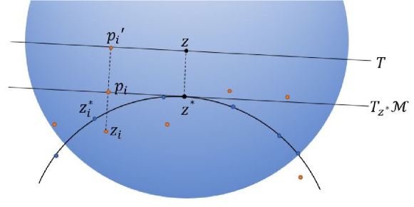
Figure 3: Diagram of variables used for the discussion of $P_{z}$.

The space $T$ is the translation of $T_{z^{*}}{\cal M}$ passing $z$, and $p_{i}^{\prime}$ is the projection of $z_{i}$ onto $T$.

Consider the symmetric matrix $\Lambda=\frac{1}{|I_{z,r^{\prime}}|}\sum_{i\in I_{z,r^{\prime}}}(p_{i}-z^{*})(p_{i}-z^{*})^{T}$. Since both $p_{i}$ and $z^{*}$ are located in $T_{z^{*}}{\cal M}$, the spanning space of $\Lambda$ is contained in $T_{z^{*}}{\cal M}$. Thus, ${\rm rank}(\Lambda)\leq{\rm dim}(T_{z^{*}}{\cal M})=d$ and thereby the $(d+1)$-th largest eigenvalue of $\Lambda$ is $0$. Setting columns of $U$ be the eigenvectors of $\Lambda$ corresponding to the $d$ largest eigenvalues, $U$ is also a basis of $T_{z^{*}}{\cal M}$. Denote $U_{\bot}$ as the orthogonal complement of $U$, and we have $\Pi_{z^{*}}^{*}=U_{\bot}U_{\bot}^{T}$. Recalling $P_{z}=V_{\bot}V_{\bot}^{T}$, where $V_{\bot}$ is the orthogonal component of $V$ and columns of $V$ are the eigenvectors corresponding to the $d$ largest eigenvalues of

$$\hat{\Lambda}=\frac{1}{|I_{z,r^{\prime}}|}\sum_{i\in I_{z,r^{\prime}}}(z_{i}-z)(z_{i}-z)^{T},$$

we obtain

$$\|P_{z}-\Pi_{z^{*}}^{*}\|_{F}=\|V_{\bot}V_{\bot}^{T}-U_{\bot}U_{\bot}^{T}\|_{F}=\|VV^{T}-\bar{U}\bar{U}^{T}\|_{F}\leq\frac{2\sqrt{2}\|\Lambda-\hat{\Lambda}\|_{F}}{\lambda_{d}}$$ (3.1)

by the following Lemma:

Lemma 8.

Let $\Lambda$, $\hat{\Lambda}\in\mathbb{R}^{n\times n}$ be symmetric, with eigenvalues $\lambda_{1}\geq\cdots\geq\lambda_{n}$ and $\hat{\lambda}_{1}\geq\cdots\hat{\lambda}_{n}$ respectively. Let $1\leq d\leq n$ and assume $\lambda_{d}>0$, $\lambda_{d+1}=0$. Let $U$, $\hat{U}\in\mathbb{R}^{n\times d}$ be eigenvectors corresponding to the first $d$ eigenvalues of $\Lambda$ and $\hat{\Lambda}$ respectively. Then

$$\|UU^{T}-\hat{U}\hat{U}^{T}\|_{F}=\sqrt{2}\|\sin\theta(\hat{U},U)\|_{F}\leq\frac{2\sqrt{2}\|\hat{\Lambda}-\Lambda\|_{F}}{\lambda_{d}}$$

by Davis-Kahan $\sin\theta$ theorem, where $\theta(\hat{U},U)$ is the $n\times n$ diagonal matrix whose diagonal consists of the principal angles between the columns spaces of $\hat{U}$ and $U$, and $\sin\theta(\hat{U},U)$ is defined entrywise.

The upper bound on $\|\hat{\Lambda}-\Lambda\|_{F}$ and the lower bound on the $d$-th eigenvalue of $\Lambda$ are required. We derive these two bounds in the following Lemma 9 and Lemma 10:

Lemma 9.

Suppose $r^{\prime}=O(\sqrt{\sigma})$ and $d(z,{\cal M})\leq cr^{\prime}$ with some $c<1$. There exists $C$ such that $\|\frac{1}{|I_{z,r^{\prime}}|}\big{(}\sum_{i\in I_{z,r^{\prime}}}(z_{i}-z)(z_{i}-z)^{T}-\sum_{i\in I_{z,r^{\prime}}}(p_{i}-z^{*})(p_{i}-z^{*})^{T}\big{)}\|_{F}$ is bounded above by

$$\frac{C}{|I_{z,r^{\prime}}|}\sum_{i\in I_{z,r^{\prime}}}\bigg{(}\|\xi_{i}\|_{2}^{4}+\|\xi_{i}\|_{2}^{3}+\|\xi_{i}\|_{2}^{2}+r^{\prime}\|\xi_{i}\|_{2}\bigg{)}+C\bigg{(}{r^{\prime}}^{3}+r^{\prime}\|z-z^{*}\|_{2}+\|z-z^{*}\|_{2}^{2}\bigg{)}.$$

Lemma 10.

The $d$-th eigenvalue of $\frac{1}{|I_{z,r^{\prime}}|}\sum_{i\in I_{z,r^{\prime}}}(p_{i}-z^{*})(p_{i}-z^{*})^{T}$ is bounded below by $\lambda_{d}\geq c{r^{\prime}}^{2}$, in probability $\delta_{0}$.

Proofs of Lemma 9 and 10 are given in Appendix A.2. Plugging the upper bound of Lemma 9 and the lower bound of Lemma 10 into (3.1), we can obtain the following theorem:

Theorem 11.

Suppose $r^{\prime}=O(\sqrt{\sigma})$ and $d(z,{\cal M})\leq r^{\prime}$. For any given $\delta$ ,there exists $C$ such that the difference between $P_{z}$ and $\Pi_{z^{*}}^{*}$ is bounded by

$$\|P_{z}-\Pi_{z^{*}}^{*}\|_{F} \leq\frac{C}{{r^{\prime}}^{2}}\frac{1}{|I_{z,r^{\prime}}|}\sum_{i\in I_{z,r^{\prime}}}\bigg{(}\|\xi_{i}\|_{2}^{4}+\|\xi_{i}\|_{2}^{3}+\|\xi_{i}\|_{2}^{2}+r^{\prime}\|\xi_{i}\|_{2}\bigg{)}$$

$$+C\bigg{(}r^{\prime}+\frac{\|z-z^{*}\|_{2}}{r^{\prime}}+\frac{\|z-z^{*}\|_{2}^{2}}{{r^{\prime}}^{2}}\bigg{)},\quad{\rm in\ probability\ }\delta_{0}.$$

The term $\|z-z^{*}\|_{2}^{2}$ in Theorem 11 tells us that $P_{z}$ cannot approximate $\Pi_{z^{*}}^{*}$ well if $z$ is far away from ${\cal M}$. However, due to the Gaussian noise and the large sample size $N$, there would always be the case that several samples are far away from the underlying manifold. Hence, the discs at sample points cannot approximate the underlying manifold well if the sample points are blurred by Gaussian noise, as we discussed in Section 1. Next section will explain that the error caused by each $P_{x_{i}}$ can be eliminated when we calculate a weighted average over $\{P_{x_{i}}\}_{i\in I_{x,r}}$, which is $\Pi_{x}$.

3.2 Properties of $\Pi_{x}$

This section evaluates how $\Pi_{x}$ approximates $\Pi_{x^{*}}^{*}$ using the upper bound of $\|P_{x_{i}}-\Pi_{x_{i}^{*}}^{*}\|_{F}$ derived in 11. As the weighted average of $\Pi_{x}$, $\Pi_{x}$ benefits from the mutual offset of the Gaussian noise. To mathematically clarify this phenomenon, the following lemma bound the weighted averages regarding $\|\xi_{i}\|_{2}$ above.

Lemma 12.

Suppose $d(x,{\cal M})\leq cr$ with some constant $c<1$ and $r=O(\sqrt{\sigma})$. For any given $\delta$, there exists constants $C$, $c_{0}$ and $n_{0}$ such that if $N\geq n_{0}r^{-d}$, then $\tilde{\alpha}(x)\geq c_{0}|I_{x,r}|$ in probability at least $(1-\delta)$ and

$$\sum_{i\in I_{x,r}}\alpha_{i}(x)\|\xi_{i}\|_{2}^{k}\leq C\sigma^{k}\quad{\rm and}\quad\frac{1}{|I_{x,r}|^{2}}\sum_{i,j\in I_{x,r}}\|\xi_{i}\|_{2}^{s}\|\xi_{i}\|_{2}^{t}\leq C\sigma^{s+t}$$ (3.2)

hold for $k,s,t\leq 4$ in probability at least $(1-\delta)^{2}$.

Lemma 13.

Suppose $x$ and $y$ are two points on ${\cal M}$ , then

$$\|\Pi_{x}^{*}-\Pi_{y}^{*}\|_{2}\leq\|\Pi_{x}^{*}-\Pi_{y}^{*}\|_{F}\leq C\frac{\|x-y\|_{2}}{\tau}.$$ (3.3)

Lemma 13 evaluates how the tangent space changes when the point of tangency changes. Proofs of the above two lemmas are given Appendix A.3. Based on these two lemmas, we have the following theorem to evaluate $\Pi_{x}$:

Theorem 14.

Suppose $d(x,{\cal M})\leq cr$ with some constant $c<1$ and $r=O(\sqrt{\sigma})$. For any given $\delta$, there exists constants $C$ and $n_{0}$ such that if $N\geq n_{0}r^{-d}$, then

$$\|\Pi_{x}-\Pi_{x^{*}}^{*}\|_{2}\leq\|\Pi_{x}-\Pi_{x^{*}}^{*}\|_{F}\leq Cr$$ (3.4)

holds in probability $\delta_{0}(1-\delta)^{2}$.

Proof  The rest of this proof is based on (3.2) and the upper bound of $\|P_{x_{i}}-\Pi_{x_{i}^{*}}^{*}\|_{F}$, which hold in probability $(1-\delta)^{2}$ and $\delta_{0}$ by Lemma 12 and Theorem 11. Hence the following statements hold in probability $\delta_{0}(1-\delta)^{2}$.

By definition of $A_{x}$,

$$\|A_{x}-\Pi_{x^{*}}^{*}\|_{F} =\bigg{\|}\sum_{i\in I_{x,r}}\alpha_{i}(x)(P_{x_{i}}-\Pi_{x_{i}^{*}}^{*})+\sum_{i}\alpha_{i}(x)(\Pi_{x_{i}^{*}}^{*}-\Pi_{x^{*}}^{*})\bigg{\|}_{F}$$

$$\leq\sum_{i\in I_{x,r}}\alpha_{i}(x)\|P_{x_{i}}-\Pi_{x_{i}^{*}}^{*}\|_{F}+\sum_{i\in I_{x,r}}\alpha_{i}(x)\|\Pi_{x_{i}^{*}}^{*}-\Pi_{x^{*}}^{*}\|_{F}$$ (3.5)

Setting $z$ in Theorem 11 to be $x_{i}$ and replacing $r^{\prime}$ by $r^{\prime}=2r$, we obtain the upper bound of $\|P_{x_{i}}-\Pi_{x_{i}^{*}}^{*}\|_{F}$. Plugging the upper bound into the first term on the right-hand side of (3.5), we obtain

$$\sum_{i\in I_{x,r}}\alpha_{i}(x)\|P_{x_{i}}-\Pi_{x_{i}^{*}}^{*}\|_{F} \leq\frac{C}{r^{2}}\sum_{i\in I_{x,r}}\sum_{j\in I_{x_{i},2r}}\frac{\alpha_{i}(x)}{|I_{x_{i},2r}|}\bigg{(}\|\xi_{j}\|_{2}^{4}+\|\xi_{j}\|_{2}^{3}+\|\xi_{j}\|_{2}^{2}+r\|\xi_{j}\|_{2}\bigg{)}$$

$$+C\bigg{(}r+\frac{\sum_{i\in I_{x,r}}\alpha_{i}(x)\|x_{i}-x_{i}^{*}\|_{2}}{r}+\frac{\sum_{i\in I_{x,r}}\alpha_{i}(x)\|x_{i}-x_{i}^{*}\|_{2}^{2}}{r^{2}}\bigg{)}$$

$$\leq\frac{C}{r^{2}}\sum_{i\in I_{x,r}}\sum_{j\in I_{x_{i},2r}}\frac{\alpha_{i}(x)}{|I_{x_{i},2r}|}\bigg{(}\|\xi_{j}\|_{2}^{4}+\|\xi_{j}\|_{2}^{3}+\|\xi_{j}\|_{2}^{2}+r\|\xi_{j}\|_{2}\bigg{)}$$

$$+C\bigg{(}r+\frac{\sum_{i\in I_{x,r}}\alpha_{i}(x)\|\xi_{i}\|_{2}}{r}+\frac{\sum_{i\in I_{x,r}}\alpha_{i}(x)\|\xi_{i}\|_{2}^{2}}{r^{2}}\bigg{)}$$

Plugging upper bound of $\sum_{i\in I_{x,r}}\alpha_{i}(x)\|\xi_{i}\|_{2}^{k}$ into the last formula leads to

$$\sum_{i\in I_{x,r}}\alpha_{i}(x)\|P_{x_{i}}-\Pi_{x_{i}^{*}}^{*}\|_{F}\leq C\Big{(}\frac{\sigma}{r}+\frac{\sigma^{2}}{r^{2}}+r\Big{)}\leq Cr.$$

And the last inequality holds given $r=O(\sqrt{\sigma})$. As for the second term,

$$\sum_{i\in I_{x,r}}\alpha_{i}(x)\|\Pi_{x_{i}^{*}}^{*}-\Pi_{x^{*}}^{*}\|_{F} \leq\frac{C}{\tau}\sum_{i\in I_{x,r}}\alpha_{i}(x)\|x_{i}^{*}-x^{*}\|_{2}$$

$$\leq\frac{C}{\tau}\sum_{i\in I_{x,r}}\alpha_{i}(x)\Big{(}\|x_{i}^{*}-x_{i}\|_{2}+\|x_{i}-x\|_{2}+\|x-x^{*}\|_{2}\Big{)}$$

$$\leq C\frac{r}{\tau}+\frac{C}{\tau}\sum_{i\in I_{x,r}}\alpha_{i}(x)\|x_{i}^{*}-x_{i}\|_{2}$$

$$\leq C\frac{r}{\tau}+C\frac{\sigma}{\tau}\leq C\frac{r}{\tau}.$$

where the first inequality is by Lemma 13. Since $\Pi_{x}$ is the closest $(D-d)$-rank projection matrix to $A_{x}$, we have

$$\|\Pi_{x}-A_{x}\|_{F}\leq\|A_{x}-\Pi_{x^{*}}^{*}\|_{F}\leq Cr.$$ (3.6)

Hence, $\|\Pi_{x}-\Pi_{x^{*}}^{*}\|_{F}\leq\|\Pi_{x}-A_{x}\|_{F}+\|A_{x}-\Pi_{x^{*}}^{*}\|_{F}\leq Cr$.

 

3.3 A bound on $f(x)$

This section discusses how $f(x)$ approximates the bias from $x$ to ${\cal M}$, which is done by calculating $\|f(x)\|_{2}$ for $x\in{\cal M}$. If $f$ approximates the bias well, such $\|f(x)\|_{2}$ should be bounded above by a small value with $x\in{\cal M}$.

Theorem 15.

Suppose $x\in{\cal M}$ and $r=O(\sqrt{\sigma})$. For any given $\delta$, there exists constants $C$ and $n_{0}$ such that if $N\geq n_{0}r^{-d}$, then $\|f(x)\|_{2}\leq Cr^{2}$ in probability $\delta_{0}(1-\delta)^{2}$.

Proof  The rest of this proof is based on (3.2) and the upper bound of $\|P_{x_{i}}-\Pi_{x_{i}^{*}}^{*}\|_{F}$, which hold in probability $(1-\delta)^{2}$ and $\delta_{0}$ by Lemma 12 and Theorem 11. Hence the following statements hold in probability $\delta_{0}(1-\delta)^{2}$. It is obvious that $x=x^{*}$ when $x\in{\cal M}$; thus we use $x$ instead of $x^{*}$ in the following discussion for convenience. First, we bound the distance between $\sum_{i\in I_{x,r}}\alpha_{i}(x)x_{i}$ and $T_{x}{\cal M}$. By definition,

$$d(\sum_{i\in I_{x,r}}\alpha_{i}(x)x_{i},T_{x}{\cal M}) =\bigg{\|}\Pi_{x}^{*}(\sum_{i\in I_{x,r}}\alpha_{i}(x)x_{i}-x)\bigg{\|}_{2}$$

$$\leq\sum_{i\in I_{x,r}}\alpha_{i}(x)\|\Pi_{x}^{*}(x_{i}-x)\|_{2}$$

$$\leq\sum_{i\in I_{x,r}}\alpha_{i}(x)\|x_{i}-x_{i}^{*}\|_{2}+\sum_{i\in I_{x,r}}\alpha_{i}(x)\|\Pi_{x}^{*}(x_{i}^{*}-x)\|_{2}$$

$$\leq\sum_{i\in I_{x,r}}\alpha_{i}(x)\|\xi_{i}\|_{2}+\sum_{i\in I_{x,r}}\alpha_{i}(x)\frac{\|x_{i}^{*}-x\|_{2}^{2}}{\tau}$$

$$\leq C_{1}\sigma+C_{2}\sum_{i\in I_{x,r}}\alpha_{i}(x)\frac{(\|x_{i}^{*}-x_{i}\|_{2}+\|x_{i}-x\|_{2})^{2}}{\tau}$$

$$\leq C_{1}\sigma+C_{2}\frac{(\sigma+r)^{2}}{\tau}.$$

The parameter $r$ is selected in the order of $\sqrt{\sigma}$, that is, there exists $C_{3}$ such that $r=C_{3}\sqrt{\sigma}>C_{3}\sigma$ since $\sigma<1$. So $(\sigma+r)^{2}<(\frac{1}{C_{3}}+1)^{2}r^{2}$ and

$$C_{1}\sigma+\frac{C_{2}}{\tau}(\sigma+r)^{2}\leq\frac{C_{1}r^{2}}{C_{3}^{2}}+\frac{C_{2}}{\tau}(\frac{1}{C_{3}}+1)^{2}r^{2}=Cr^{2}.$$

Hence, we obtain $d(\sum_{i\in I_{x,r}}\alpha_{i}(x)x_{i},T_{x}{\cal M})\leq Cr^{2}$.

We let $a=\sum_{i\in I_{x,r}}\alpha_{i}(x)x_{i}$ and $b$ be the projection of $a$ onto $T_{x}{\cal M}$. Then, we have

$$\|a-b\|_{2}=\|\Pi_{x}^{*}(a-b)\|_{2}=d\bigg{(}\sum_{i\in I_{x,r}}\alpha_{i}(x)x_{i},T_{x}{\cal M}\bigg{)}\leq Cr^{2}.$$

According to the definition of $f(x)$,

$$f(x)=\Pi_{x}(x-a)=\Pi_{x}^{*}(x-b)+(\Pi_{x}-\Pi_{x}^{*})(x-b)+\Pi_{x}(b-a),$$

where $\Pi_{x}^{*}(x-b)=\bf{0}$, since $x=x^{*}\in T_{x}{\cal M}$ and $b\in T_{x}{\cal M}$. Hence, we obtain

$$\|f(x)\|_{2} \leq\|\Pi_{x}-\Pi_{x}^{*}\|_{F}\big{(}\|x-a\|_{2}+\|a-b\|_{2}\big{)}+\|\Pi_{x}(a-b)\|_{2}$$

$$\leq\|\Pi_{x}-\Pi_{x}^{*}\|_{F}\big{(}\|x-a\|_{2}+\|a-b\|_{2}\big{)}+\|a-b\|_{2}$$

$$\leq C_{1}r\times(r+r^{2})+C_{2}r^{2}\leq Cr^{2}.$$

 

3.4 A bound on the first and second derivative of $f(x)$

We now proceed to obtain an upper bound on $\|\partial_{v}f(x)\|_{2}$ with $\|v\|_{2}=1$, where

$$\partial_{v}f(x)=\lim_{t\to 0}\frac{f(x+tv)-f(x)}{t},$$

for any $v\in\mathbb{R}^{D}$. Lemma 16, Lemma 17 and Theorem 18 complete the derivation of such upper bound. Lemma 16 and Lemma 17 are proved in Appendix A.4.

Lemma 16.

Suppose $d(x,{\cal M})\leq cr$ with some constant $c<1$ and $r=O(\sqrt{\sigma})$. For any given $\delta$, there exists constants $C$ and $n_{0}$ such that if $N\geq n_{0}r^{-d}$, then the following inequalities hold:

• $\|\big{(}\|P_{x_{i}}-\Pi_{x_{i}^{*}}\|_{2}\big{)}_{i\in I_{x,r}}\|_{2}\leq Cr|I_{x,r}|^{\frac{1}{2}}$ in probability $\delta_{0}(1-\delta)^{2}$,

• $\|\big{(}\|x_{i}-x_{i}^{*}\|_{2}\big{)}_{I_{x,r}}\|_{2}\leq Cr^{2}|I_{x,r}|^{\frac{1}{2}}$ in probability $1-\delta$,

• $\|\big{(}\|x_{i}^{*}-x^{*}\|_{2}\big{)}_{I_{x,r}}\|_{2}\leq Cr|I_{x,r}|^{\frac{1}{2}}$ in probability $1-\delta$.

Lemma 17.

Suppose $d(x,{\cal M})\leq cr$ with some constant $c<1$, $r=O(\sqrt{\sigma})$ and $\beta\geq 2$. For any given $\delta$, there exists constants $C$ and $n_{0}$ such that if $N\geq n_{0}r^{-d}$, then

$$\|\big{(}\partial_{v}\alpha_{i}(x)\big{)}_{i\in I_{x,r}}\|_{2}\leq\frac{C}{r}|I_{x,r}|^{-\frac{1}{2}}\ {\mbox{w}ith\ probability}\ 1-\delta.$$

Theorem 18.

Suppose $d(x,{\cal M})\leq cr$ and $r=O(\sqrt{\sigma})$. For any given $\delta$, there exists constants $C$ and $n_{0}$ such that if $N\geq n_{0}r^{-d}$,

$$\|\partial_{v}f(x)-\Pi_{x}v\|_{2}\leq Cr,$$ (3.7)

in probability $\delta_{0}(1-\delta)^{2}$.

Based on previous lemma, we achieve Theorem 18, which claims the first derivative of $f(x)$ approximates $\Pi_{x}v$ in the order of $O(r)$. The proof of Theorem 18 refers to Appendix A.5. We now proceed to obtain an upper bound on $\|\partial_{v}\big{(}\partial_{u}f(x)\big{)}\|_{2}$ with $\|v\|_{2}=\|u\|_{2}=1$ in Theorem 20. Its proof is based on Lemma 19, which is proved in Appendix A.4.

Lemma 19.

Suppose $d(x,{\cal M})\leq cr$ with some constant $c<1$, $r=O(\sqrt{\sigma})$ and $\beta\geq 2$. For any given $\delta$, there exists constants $C$ and $n_{0}$ such that if $N\geq n_{0}r^{-d}$, then

$$\Big{\|}\big{(}\partial_{v}\partial_{u}\alpha_{i}(x)\big{)}_{i\in I_{x,r}}\Big{\|}_{2}\leq\frac{C}{r^{2}}|I_{x,r}|^{-\frac{1}{2}}\ {\mbox{w}ith\ probability}\ 1-\delta.$$

Theorem 20.

Suppose $d(x,{\cal M})\leq cr$ with some constant $c<1$ and $r=O(\sqrt{\sigma})$. For any given $\delta$, there exists constants $C$ and $n_{0}$ such that if $N\geq n_{0}r^{-d}$, then $\|\partial_{v}\partial_{u}f(x)\|_{2}\leq C$ in probability $\delta_{0}(1-\delta)^{2}$.

Theorem 20 proves that the second derivative of $f(x)$ is bounded above by certain constant, which indicates the smoothness of $f(x)$. The proof of Theorem 20 also refers to Appendix A.5.

4 Proofs of Theorem 4, Theorem 5 and Theorem 7

The proof of Theorem 4 requires the equivalence in Proposition 21, which is proved in Appendix A.6.

Proposition 21.

Let $h(z):B_{D}(x,\epsilon)\subset\mathbb{R}^{D}\to\mathbb{R}^{D-d}$, per

$$h(z)=V_{x}^{T}f(z),$$ (4.1)

where $V_{x}$ is the factor of $\Pi_{x}$ such that $\Pi_{x}=V_{x}V_{x}^{T}$. Then $h^{-1}({\bf 0})=B_{D}(x,\epsilon)\cap f^{-1}({\bf 0})$ in the probability $\delta_{0}(1-\delta)^{2}\big{(}1-(1-cr^{d})^{N}\big{)}$.

Proof (Proof of Theorem 4) This proof requires $h^{-1}({\bf 0})=B_{D}(x,\epsilon)\cap f^{-1}({\bf 0})$, $\|J_{f}(x)-\Pi_{x}\|_{F}\leq Cr$ in (4.2) and $\|J_{f}(z)-J_{f}(x)\|_{F}\leq Cr$ in (4.3). By Proposition 21, $h^{-1}({\bf 0})=B_{D}(x,\epsilon)\cap f^{-1}({\bf 0})$ is based on $\|\Pi_{x}-\Pi_{z}\|_{2}\leq Cr$ for $z\in B_{D}(x,\epsilon)$ by Proposition 29, while Proposition 29 is based on Theorem 14 and Proposition 28(ii). Among the metioned conclusions, Theorem 14, (4.2) and (4.3) hold when Lemma 12 and Theorem 11 hold. Hence, the following statements hold when Lemma 12, Theorem 11 and Proposition 28(ii) simultaneously hold, with probability $\delta_{0}(1-\delta)^{2}\big{(}1-(1-cr^{d})^{N}\big{)}$. For simplicity, we omit the discussion on the probability in subsequent proofs without confusion.

For $z\in B_{D}(x,\epsilon)$,

$$J_{h}(z) =V_{x}^{T}J_{f}(z)$$

$$=V_{x}^{T}(J_{f}(z)-J_{f}(x))+V_{x}^{T}(J_{f}(x)-\Pi_{x})+V_{x}^{T}\Pi_{x}.$$

Recalling $\|J_{f}(x)-\Pi_{x}\|_{F}\leq Cr$ and $\|J_{f}(z)-J_{f}(x)\|_{F}\leq Cr$ in accordance with (4.2) and (4.3), and $V_{x}^{T}\Pi_{x}=V_{x}^{T}$, we have

$$\|J_{h}(z)-V_{x}^{T}\|_{2}\leq\|J_{h}(z)-V_{x}^{T}\|_{F}\leq Cr.$$

Hence, the maximal difference between the singular values of $J_{h}(z)$ and $V_{x}^{T}$ is bounded by $Cr$. Let $\sigma_{1}\geq\cdots\geq\sigma_{D-d}$ be the singular values of $J_{h}(z)$. We obtain $|\sigma_{D-d}-1|\leq Cr$ since the singular values of $V_{x}^{T}$ are $1$, which implies $\sigma_{D-d}\geq 1-Cr$ and ${\rm rank}\big{(}J_{h}(z)\big{)}=D-d$ for any $z\in B_{D}(x,\epsilon)$.

This means the rank of $h$ at $z$ equals to $D-d$ for any $z\in B_{D}(x,\epsilon)$, and thereby $h^{-1}(\bf{0})$ is a $d$-dimensional submanifold of $B_{D}(x,\epsilon)\subset\mathbb{R}^{D}$. The equivalence between $h^{-1}(\bf{0})$ and $f^{-1}(\bf{0})$ in $B_{D}(x,\epsilon)$ by Proposition 21 guarantees $f^{-1}(\bf{0})$ is also a $d$-dimensional submanifold of $B_{D}(x,\epsilon)\subset\mathbb{R}^{D}$.  

Proof (Proof of Theorem 5) This proof requires $\|f(x^{*})\|_{2}\leq Cr^{2}$, $\|\Pi_{x}-\Pi_{x^{*}}^{*}\|_{F}\leq Cr$, $\|\partial_{v}f(x)-\Pi_{x}v\|_{2}\leq Cr$ and $\|J_{f}(x^{\prime})-J_{f}(x^{\prime\prime})\|_{F}\leq C\|x^{\prime}-x^{\prime\prime}\|_{2}$. By the proofs of Theorem 14, Theorem 15, Theorem 18 and Theorem 20, these requirements simultaneously hold when the inequalities of Lemma 12 and Theorem 11 hold. We assume inequalities of Lemma 12 and Theorem 11 hold, in probability $\delta_{0}(1-\delta)^{2}$. Hence, the following statements hold in probability $\delta_{0}(1-\delta)^{2}$. For simplicity, we omit the discussion on the probability in subsequent proofs without confusion.

For any fixed $x\in{\cal M}_{\rm out}$, we let $V_{x}\in\mathbb{R}^{D\times(D-d)}$ denote the orthonormal matrix such that $\Pi_{x}=V_{x}V_{x}^{T}$, and let $U_{x}$ denote the orthogonal complement of $V_{x}$. Then, we define

$${{\color[rgb]{0,0,0}F(z)=f(z)+U_{x}U_{x}^{T}z.}}$$

Let $x^{*}$ be the projection of $x$ onto ${\cal M}$, as done previously, $\Pi_{x^{*}}^{*}=V_{*}V_{*}^{T}$, and $U_{*}$ be the orthogonal complement of $V_{*}$. The difference $\|F(x^{*})-F(x)\|_{2}$ can be evaluated as

$$\|F(x^{*})-F(x)\|_{2}$$

$$= \|f(x^{*})+U_{x}U_{x}^{T}x^{*}-f(x)-U_{x}U_{x}^{T}x\|_{2}$$

$$= \|f(x^{*})+U_{x}U_{x}^{T}x^{*}-U_{x}U_{x}^{T}x\|_{2}$$

$$\leq \|f(x^{*})\|_{2}+\|(U_{x}U_{x}^{T}-U_{*}U_{*}^{T})(x-x^{*})\|_{2}+\|U_{*}U_{*}^{T}(x-x^{*})\|_{2}$$

$$= \|f(x^{*})\|_{2}+\|(\Pi_{x}-\Pi_{x^{*}}^{*})(x-x^{*})\|_{2}+\|U_{*}U_{*}^{T}(x-x^{*})\|_{2}$$

$$\leq \|f(x^{*})\|_{2}+\|\Pi_{x}-\Pi_{x^{*}}^{*}\|_{F}\|x-x^{*}\|_{2}+\|U_{*}U_{*}^{T}(x-x^{*})\|_{2}$$

$$\leq Cr^{2}$$

The second equality holds because $f(x)=\bf{0}$ for $x\in{\cal M}_{\rm out}$. And the last inequality holds because $\|f(x^{*})\|_{2}\leq Cr^{2}$ via Theorem 15, $\|\Pi_{x}-\Pi_{x^{*}}^{*}\|_{F}\leq Cr$ via Theorem 14, $\|x-x^{*}\|=d(x,{\cal M})\leq cr$ via the definition of ${\cal M}_{\rm out}$, and $U_{*}U_{*}^{T}x=U_{*}U_{*}^{T}x^{*}$, since $x^{*}$ is the projection of $x$ onto $T_{x^{*}}{\cal M}$.

The Jacobian matrix of $F$ at $z=x$, denoted by $J_{F}(x)$ for simplicity, is

$$J_{F}(x)=J_{f}(x)+U_{x}U_{x}^{T}=I_{D}+\big{(}J_{f}(x)-\Pi_{x}\big{)}.$$

In accordance with the definition of $\partial_{v}f(x)$ and $\|\partial_{v}f(x)-\Pi_{x}v\|_{2}\leq Cr$ by Theorem 18,

$$J_{f}(x)-\Pi_{x}=\big{(}\partial_{e_{1}}f(x),\cdots,\partial_{e_{D}}f(x)\big{)}-\big{(}\Pi_{x}e_{1},\cdots,\Pi_{x}e_{D}\big{)},$$

where $e_{i}$ is the $i$-th column of $I_{D}$. Thus, the length of the $i$-th column of $J_{f}(x)-\Pi_{x}$, that is, $\partial_{e_{i}}f(x)-\Pi_{x}e_{i}$, is less than $Cr$. Hence,

$$\|J_{f}(x)-\Pi_{x}\|_{2}\leq Cr,\quad{\rm and}\quad J_{F}(x)=I_{D}+O(r),$$ (4.2)

which means that $J_{F}(x)$ approximates $I_{D}$ and $J_{F}(x)$ is invertible. Moreover, $\|J_{F}(x)\|_{F}\leq C(1+r)$ and its inversion is $\|J_{F}^{-1}(x)\|_{F}\leq C(1+r)$.

The changing rate of $J_{F}$ can also be bounded as follows: supposing $x^{\prime}$ and $x^{\prime\prime}$ are two arbitrary points, we have

$$\|J_{F}(x^{\prime})-J_{F}(x^{\prime\prime})\|_{F}=\|J_{f}(x^{\prime})-J_{f}(x^{\prime\prime})\|_{F}\leq C\|x^{\prime}-x^{\prime\prime}\|_{2}$$ (4.3)

by the upper bound on the second derivative of $f(x)$ in Theorem 20.

Based on the conclusions that $\|F(x)-F(x^{*})\|_{2}\leq Cr^{2}$, $J_{F}(x)=I_{D}+O(r)$, and $\|J_{F}(x^{\prime})-J_{F}(x^{\prime\prime})\|_{F}\leq C\|x^{\prime}-x^{\prime\prime}\|_{2}$, we could bound $\|x-x^{*}\|_{2}$ via Theorem 2.9.4 (the inverse function theorem) in Hubbard and Hubbard (2001). Specifically,

$$\|x-x^{*}\|_{2}\leq Cr^{2}.$$

 

For any fixed point $x\in{\cal M}_{\rm out}$, set $W_{x}$ to be the basis of the spanning space of $J_{f}(x)^{T}$. Since the rows of $J_{f}(x)$ are orthogonal to the contour surface at $x$, $W_{x}$ is also the basis of the normal space of ${\cal M}_{\rm out}$ at $x$ and thereby $W_{x}\in\mathbb{R}^{D\times(D-d)}$ by Theorem 4. Based on $W_{x}$, we construct a function $g(z):\mathbb{R}^{D}\to\mathbb{R}^{D-d}$, per

$$g(z)=W_{x}^{T}f(z).$$ (4.4)

As shown in the following proposition, $f^{-1}(\bf{0})$ and $g^{-1}(\bf{0})$ also describe the same set in the neighborhood of $x$.

Proposition 22.

Given $z\in B_{D}(x,r\tau)$, $g(z)=\bf{0}$ if and only if $f(z)=\bf{0}$ in probability at least $\delta_{0}^{2}(1-\delta)^{4}\big{(}1-(1-cr^{d})^{N}\big{)}$.

The proof can be found in Appendix A.6. By $W_{x}$, we reset the coordinate system. Specifically, we set the first $d$ coordinates as the basis of $T_{x}{\cal M}_{\rm out}$ and the last $D-d$ coordinates as the columns of $W_{x}$. In this coordinate system, we define an implicit function $\phi:\mathbb{R}^{d}\to\mathbb{R}^{D-d}$ based on $g(\cdot)$ using the implicit function theorem, such that $\big{(}\zeta;\phi(\zeta)\big{)}$ maps $\zeta\in T_{x}{\cal M}_{\rm out}$ to a point on the manifold ${\cal M}_{\rm out}$. Here, we denote $(\eta;\zeta)$ as the concatenation of column vector $\eta$ and $\zeta$. The upper bound on the first and second derivatives of $\phi$ is given in Lemma 23, the proof of which can be found in Appendix A.6.

Lemma 23.

Suppose function $g$ is defined as (4.4). The implicit function $\phi:\mathbb{R}^{d}\to\mathbb{R}^{D-d}$ satisfying $g\big{(}\cdot,\phi(\cdot)\big{)}=\bf{0}$ exists, and its first and second derivatives are bounded above by

$$\partial_{s}\phi(\zeta)\leq C\|\big{(}\zeta;\phi(\zeta)\big{)}-x\|_{2},\quad\partial_{t}\partial_{s}\phi(\zeta)\leq C,$$

in probability at least $\delta_{0}(1-\delta)^{2}\big{(}1-(1-cr^{d})^{N}\big{)}$, for any $\|s\|_{2}=\|t\|_{2}=1$.

Proof (Proof of Theorem 7) This proof requires the claims of Proposition 22 and Lemma 23 simultaneously hold, which is in probability $\delta_{0}^{2}(1-\delta)^{4}\big{(}1-(1-cr^{d})^{N}\big{)}$ by the proofs of Proposition 22 and Lemma 23. Hence the following statements hold in probability at least $\delta_{0}^{2}(1-\delta)^{4}\big{(}1-(1-cr^{d})^{N}\big{)}$. For simplicity, we omit the discussion on the probability in subsequent proofs without confusion.

Let $x$ and $z$ be two points on ${\cal M}_{\rm out}$, and $T_{x}{\cal M}_{\rm out}$ be the tangent space to ${\cal M}_{\rm out}$ at $x$. The proof is conducted with $\|z-x\|_{2}>r\tau$ and $\|z-x\|_{2}\leq r\tau$ respectively. First, when $\|z-x\|_{2}>r\tau$,

$$\frac{\|z-x\|_{2}^{2}}{d(z,T_{x}{\cal M}_{\rm out})}\geq cr\tau$$ (4.5)

holds because $\|z-x\|_{2}\geq d(z,T_{x}{\cal M}_{\rm out})$. Second, when $\|z-x\|_{2}\leq r\tau$, we have $g(z)=f(z)=g(x)=f(x)=\bf{0}$ by Proposition 22 in probability $\delta_{0}^{2}(1-\delta)^{4}\big{(}1-(1-cr^{d})^{N}\big{)}$, since $x$ and $z$ are on ${\cal M}_{\rm out}$. Let $\zeta_{x}$ and $\zeta_{z}$ denote the first $d$ coordinates of $x$ and $z$, respectively. We have $z=\big{(}\zeta_{z};\phi(\zeta_{z})\big{)}$, $x=\big{(}\zeta_{x};\phi(\zeta_{x})\big{)}$, $\partial_{s}\phi(\zeta_{z})\leq C\|z-x\|_{2}$ and $\partial_{t}\partial_{s}\phi(\zeta_{z})\leq C$ in probability at least $\delta_{0}(1-\delta)^{2}$ by Lemma 23. So,

$$d(z,T_{x}{\cal M}_{\rm out}) =\|\phi(\zeta_{z})-\phi(\zeta_{x})\|_{2}$$

$$\leq C\|z-x\|_{2}\|\zeta_{z}-\zeta_{x}\|_{2}+C\|\zeta_{z}-\zeta_{x}\|_{2}^{2}$$

$$\leq C\|z-x\|_{2}^{2}+C\|z-x\|_{2}^{2}\leq C\|z-x\|_{2}^{2}.$$

As a result,

$$\frac{\|z-x\|_{2}^{2}}{d(z,T_{x}{\cal M}_{\rm out})}\geq\frac{\|z-x\|_{2}^{2}}{C\|z-x\|_{2}^{2}}=c.$$

Combining with (4.5), we complete this proof.  

5 Experiment Results

This section consists of two parts. The first part provides numerical comparisons with the methods in Mohammed and Narayanan (2017), Fefferman et al. (2018), and Aizenbud and Sober (2021). We implement relevant methods on several known manifolds, illustrate the output manifolds, and calculate the Hausdorff distances between the output and underlying manifolds. In the second part, we focus on real applications, and use our method to denoise facial images sampled from a long video. The results of our method are then contrasted with those of the other methods.

Implementation: the MATLAB codes together with all numerical examples used in this paper are available on https://zhigang-yao.github.io/research.html which contains a GitHub link under the code tab. We have also implemented the related methods from Mohammed and Narayanan (2017) and Fefferman et al. (2018), since the authors of both papers have not provided implementation due to the nature of their work has been purely abstract.

5.1 Simulation

Input: a point $x$, noisy data $X=[x_{1},\cdots,x_{N}]$, a bandwidth parameter $r$, a step length parameter $a$, a tolerance $\epsilon$, and the maximal number of iteration $T$.

Output: projection $\tilde{x}$ of $x$ onto ${\cal M}_{\rm out}$.

• Calculate $P_{x_{i}}=I-VV^{T}$ for each $x_{i}\in X$, where $V$ is the $D\times d$ matrix whose columns are the eigenvectors corresponding to the largest $d$ eigenvectors of $\sum_{j\in I_{x_{i},2r}}(x_{j}-x_{i})(x_{j}-x_{i})^{T}$.

• Set $t=1$.

  • Calculate $\tilde{\alpha}_{i}(x)$ and $\alpha_{i}(x)$ for $i\in I_{x,r}$ by (2.4).

  • Plug $\{\tilde{\alpha}_{i}(x),\alpha_{i}(x),P_{x_{i}}\}_{i\in I_{x,r}}$ into (B.1) to obtain the gradient ${\rm grad}(x)$ of $\|f(x)\|_{2}^{2}$.

  • Update $t=t+1$ and $x=x-a\cdot{\rm grad}(x)$.

  • Repeat (1) to (3) until the tolerance condition $\|f(x)\|_{2}^{2}\leq\epsilon$ or the maximal iteration $T$ is met.

• Output $\tilde{x}=x$.

Algorithm 1 Project $x$ onto ${\cal M}_{\rm out}$

As explained in Subsection 1.2, by removing the unreliable discs which centered at the sample points as in Mohammed and Narayanan (2017) and Fefferman et al. (2018), one would expect better performance than from these two methods. Assuming the data points are sampled from a tubular neighborhood, Aizenbud and Sober (2021) denoises the sample points iteratively using an local polynomial regression. As the degree increases, polynomial regression fits a manifold better when the noise is limited. However, a polynomial regression is sensitive once the noise increases. As a method designed for Gaussian noise, our method is expected to be more robust when the noise increases. To support the claim, we test methods in Mohammed and Narayanan (2017) (marked by km17), Fefferman et al. (2018) (marked by cf18), and Aizenbud and Sober (2021) with polynomial degree 1 and 2 (marked by ya21(deg=1) and ya21(deg=2)) on manifolds with both constant and inconstant curvature, namely: a circle embedded in $\mathbb{R}^{2}$, a sphere embedded in $\mathbb{R}^{3}$, and a torus embedded in $\mathbb{R}^{3}$. To have a traceable comparison, all the tests are conducted in the following way, similar to that of Mohammed and Narayanan (2017):

• Sample $N$ points from the underlying manifold, blur the points with Gaussian noise defined in (1.1) with given $\sigma$, and use the noisy data $X=[x_{1},\cdots,x_{N}]$ to implicitly construct output manifolds.

• Initialize a collection of points $P=[p_{1},\cdots,p_{N_{0}}]$ around the underlying manifold.

• Project each $p_{i}$ to the constructed output manifolds via km17, cf18, ya21(deg=1), ya21(deg=2)) and our method, respectively. We will then obtain $\tilde{P}$ as the projection of $P$ for each method.

• Calculate the Hausdorff distance between each $\tilde{P}$ and ${\cal M}$ to estimate the Hausdorff distance between the corresponding ${\cal M}_{\rm out}$ and ${\cal M}$.

As projections, points in $\tilde{P}$ lie on the corresponding ${\cal M}_{\rm out}$, and the Hausdorff distance $H(\tilde{P},{\cal M})$ could estimate $H({\cal M}_{\rm out},{\cal M})$ when $\tilde{P}$ are dense enough. This motivates us to evaluate the approximation error of ${\cal M}_{\rm out}$ to ${\cal M}$ by $H(\tilde{P},{\cal M})$. To project a point $p$ onto a manifold defined by (2.6), we design algorithm 1. Taking $x=p$ and $f$ in algorithm 1 as (2.5), we could project $p$ onto our output manifold. It should be noted that the difficulty of calculating such a gradient lies in calculating a gradient of orthogonal projection, which can be addressed according to Shapiro and Fan (1995). Detailed formula refers to Appendix B. Mohammed and Narayanan (2017) suggested a subspace-constrained gradient descent algorithm to project a point onto ${\cal M}_{\rm out}$ constructed by km17. Thus, we adopt this algorithm to implement km17 in this simulation. Although Fefferman et al. (2018) have not considered the issue, we implement their method too via algorithm 1, treating $f(x)$ as the approximated bias at $x$ defined by Fefferman et al. (2018).

The details of this simulation are as follows: we uniformly sample $N$ points denoted by $y_{1},\cdots,y_{N}$ from each target manifold and i.i.d. sample $\xi_{1},\cdots,\xi_{N}$ from a Gaussian distribution (1.1) with a given standard derivation $\sigma$. Then, the noisy data $X=\{x_{i}\}_{i=1}^{N}$ is constructed by $x_{i}=y_{i}+\xi_{i}$. The initial points $P$ are sampled from the tube centered at ${\cal M}$ with radius $\frac{1}{2}\sqrt{\frac{\sigma}{D}}$, so that $d(p_{i},{\cal M})\leq\sqrt{\sigma}$ for each $p_{i}$. According to Theorem 5, $d(\tilde{p}_{i},{\cal M})\leq O(\sigma)$, which means the output points should be much closer to the underlying manifold than the initial points. Again, we take $N_{0}=N$ initial points for each test in the simulation.

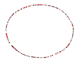
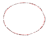
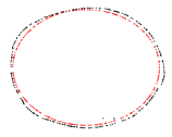
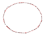
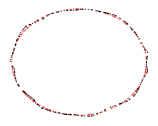
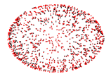
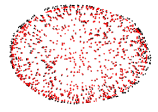
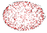
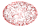
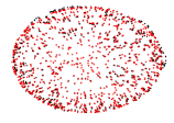
Figure 4: Performances of our method, km17, cf18, ya21(deg=1) and ya21(deg=2) when fitting a circle (top row) and a sphere (bottom row), where black points represent points in $\tilde{P}$(black dots) and red points represents their projections onto ${\cal M}$.

To implicitly construct the output manifolds, the methods–km17, cf18, and our method–require a bandwidth parameter $r$. According to the theoretical analysis, $r=O(\sqrt{\sigma})$. So we take $r=\lambda\sqrt{\sigma}$ in this simulation, where $\lambda$ is tuned in a large range for each method and each $\sigma$. All the results reported in this section are the ones using the best $\lambda$. The method ya21 also requires a bandwidth parameter $h$, which is again selected as the best one tuned from a large range. In constructing $\tilde{\alpha}_{i}(x)$, our method requires $\beta\geq 2$. We take $\beta=d+2$ in the simulation, which is same as Fefferman et al. (2018) did.

5.1.1 Manifold with constant curvature

This part tests the manifold fitting methods for the circle in $\mathbb{R}^{2}$ and the sphere embedded in $\mathbb{R}^{3}$. For the circle case, we set $N=N_{0}=300$, while for the sphere case, we set $N=N_{0}=1000$. The different setting of sample-size guarantees the similar density in both cases, as Figure 4 shows. Figure 4 illustrates that the $\tilde{P}$ (black dots) and their projection onto ${\cal M}$ (red dots) obtained by our method, cf18, cf18, ya21(deg=1) and ya21(deg=2), from left to right. The black dots and red dots can be treated as the discretized versions of ${\cal M}_{\rm out}$ and ${\cal M}$ respectively. Thus, a larger overlap of the two sets of dots means the manifold is better fitted. For the circle embedded in $\mathbb{R}^{2}$, we show the entire space in the left column, while for the sphere embedded in $\mathbb{R}^{3}$, we show the view from the positive $z$ axis. Figure 4 shows that km17 obviously performs worse than the other methods in terms of fitting error. From the two estimated circles by ya21(deg=1) and ya21(deg=2), we observe that there are sharp corners at the both top left and bottom right. This observation verifies that the estimator by ya21 is not smooth. From the right edge of the circle and the sphere, we can also see that our method preforms slightly better than cf18 in this experiment.

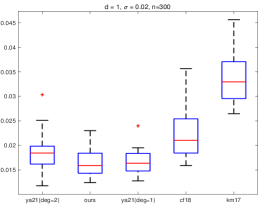
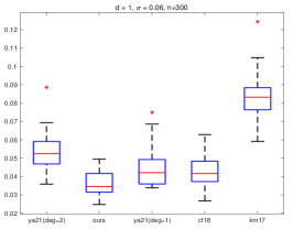
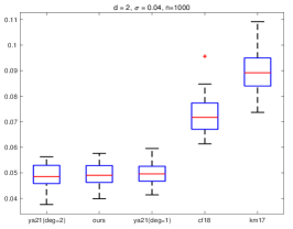
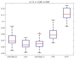
Figure 5: The Hausdorff distance of fitting a circle (top row) and a sphere (bottom row) with $\sigma=0.02$ (left column), $\sigma=0.04$ (middle column) and $\sigma=0.06$ (right column) using ya21(deg=2), our method, ya21(deg=1), cf18 and km17 respectively.

To confirm the advantage of our method, we repeat each test for 20 trials, and list the results of $H(\tilde{P},{\cal M})$ using the different methods in Figure 5. Generally speaking, our method outperforms cf18, km17 and ya21(deg=1) in the compared cases. Although ya21(deg=2) performs slightly better than our method in the cases of very small noise, it is much more sensitive than our method. As the $\sigma$ increases, ya21(deg=2) fails to outperform other methods. From Figure 5, $H({\cal M},{\cal M}_{\rm out})=O(\sigma)$ for our method, which supports Theorem 5.

5.1.2 Manifold with inconstant curvature

We also implement the compared methods in the torus case, which is a type of manifold with inconstant curvature. Figure 6 illustrates the case with $N=N_{0}=800$ and $\sigma=0.04$, and the torus embedded in $\mathbb{R}^{3}$ is shown from the positive z axis. Here, the sample points in $\tilde{P}$ are marked by black dots and their projection onto ${\cal M}$ are marked by red dots. The five subfigures are obtained by our method, cf18, km17, ya21(deg=1) and ya21(deg=2), from left to right. From the top and right edge of the torus, we can observe that our method performs better than cf18 and km17. From the fourth subfigure, we can tell an obvious gap between the red and black dots around the edge of the torus, which means ya21(deg=1) failed to fit these points. Using a second degree polynomial, ya21(deg=2) achieves better fitting as the right subfigure shows.

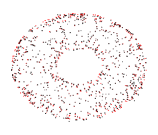
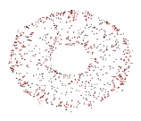
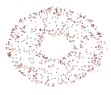
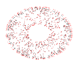
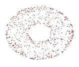
Figure 6: Performances of our method, km17, cf18, ya21(deg=1) and ya21(deg=2) when fitting a torus with $N=N_{0}=800$ and $\sigma=0.04$, where black points represent points in $\tilde{P}$(black dots) and red points represents their projections onto ${\cal M}$.

We also repeat each test for 20 trials and list the the results of $H(\tilde{P},{\cal M})$ using the different methods in Figure 7. When $\sigma=0.02$ and $\sigma=0.04$, our method performs better than cf18, km17 and ya21(deg=1). As $\sigma$ increases to $0.06$, the fitting problem is more difficult and the performance of km17, cf18 and our method are similar. This case further demonstrates the sensitivity of ya21(deg=2). When $\sigma$ is small and the sample size is adequate, ya21(deg=2) outperforms the other methods. However, when the sample size decreases and $\sigma$ increases, the performance of ya21(deg=2) deteriorates rapidly.

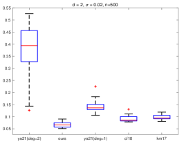
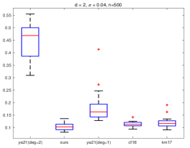
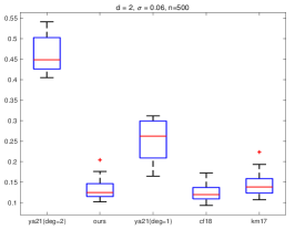
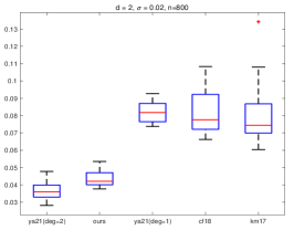
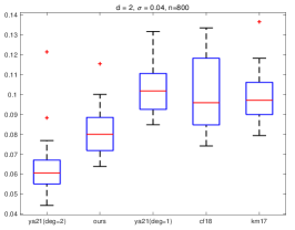
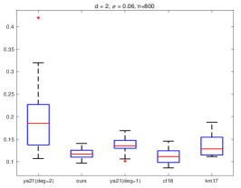
Figure 7: The Hausdorff distance of fitting a torus given 500 (top row) and 1000 (bottom row) samples with $\sigma=0.02$ (left column), $\sigma=0.04$ (middle column) and $\sigma=0.06$ (right column) using ya21(deg=2), our method, ya21(deg=1), cf18 and km17 respectively.

5.2 Facial image denoising

This subsection considers a concrete case–denoising facial images selected from the video database in Happy et al. (2012). We select 1000 images of an individual turning his head around, and blur images via Gaussian distribution with a different standard derivation $\sigma$. In this experiment, $\sigma$ is set to be the average of all pixels in 1000 images multiplied by $\rho=0.2,0.3$, or $0.4$. The size of each facial image is $80\times 80$, which means $D=6400$. The dimension $d$ of the underlying manifold is tuned from $\{1,5,10,15,20,50,75,100\}$ for each method and we choose $d=10$ because of its outperformance.

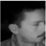
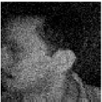
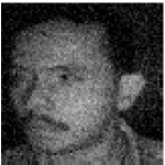
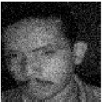
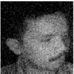
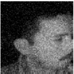
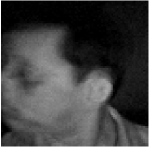
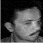
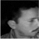
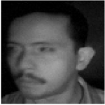
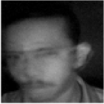
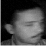
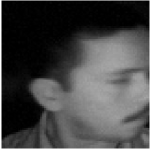
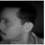
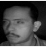
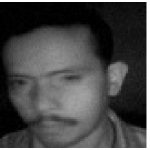
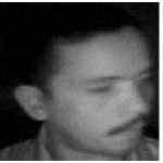
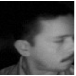
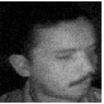
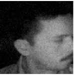
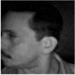
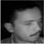
Figure 8: Performance of facial image denoising with $\rho=0.3$. The first row consists of original images, and the second row consists of blurred images. The third to the seventh rows contain deblurred images using km17, cf18, ya21(deg=1), ya21(deg=2) and our method, respectively.

From the 1000 facial images, we select 5 with different head orientations. The top row of Figure 8 exhibits these five original images, and the second row of Figure 8 exhibits these five images blurred, with $\rho=0.3$. The goal of this experiment is to denoise these five blurred images by projecting them to the manifold underlying the remaining 995 blurred images, which are treated as the noisy samples. To achieve the denoising, we use km17, cf18, ya21(deg=1), ya21(deg=2) and our method to construct the output manifold with the 995 noisy samples, and project the five tested images to each output manifold. When the output manifold correctly fits the underlying one, projecting blurred images to the output manifold denoises these facial images. In this experiment, we take $\beta=2$ for our method to construct $\tilde{\alpha}_{i}(x)$. If cf18 uses $\tilde{\alpha}_{i}(x)$ as Fefferman et al. (2018) has suggested, it would work quite unsatisfactorily, because of using the over-large power $d+2$ rather than $\beta$. Therefore, we take the same $\tilde{\alpha}_{i}(x)$ for cf18 and our method to make the results comparable.

The last three rows of Figure 8 show the denoised images obtained by km17, cf18, ya21(deg=1), ya21(deg=2) and our method, respectively. The first and third facial images were not recovered by km17. Although the faces in the other three images obtained by km17 can be distinguished, they are still very noisy. Cf18 could not recover the third image either, although the other four images obtained by cf18 are better than the ones obtained by km17. Both ya21(deg=1) and ya21(deg=2) can recover these five faces. However, the faces obtained by ya21(deg=2) are still somewhat fuzzy, compared with the ones obtained by ya21(deg=1) and our method. Our method recovered all the five faces, with the third face of much better quality than the faces from km17 and cf18.

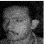
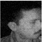
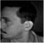
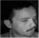
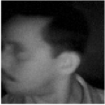
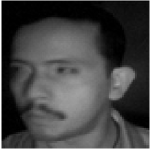
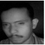
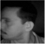
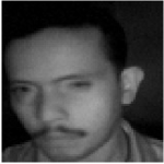
Figure 9: Performance of facial image denoising with $\rho=0.2$. The first row consists of original images, and the second row consists of blurred images. The third to the seventh rows contain deblurred images using km17, cf18, ya21(deg=1), ya21(deg=2) and our method, respectively.

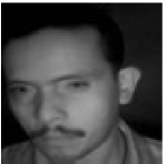
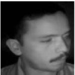
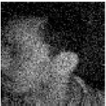
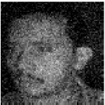
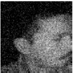
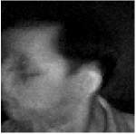
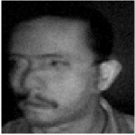
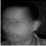
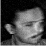
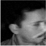
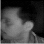
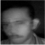
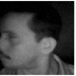
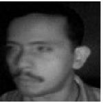
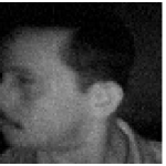
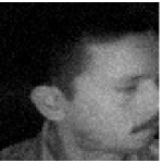
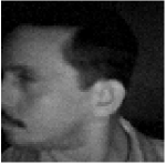
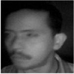
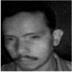
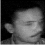
Figure 10: Performance of facial image denoising with $\rho=0.4$. The first row consists of original images, and the second row consists of blurred images. The third to the seventh rows contain deblurred images using km17, cf18, ya21(deg=1), ya21(deg=2) and our method, respectively.

The results with the settings $\rho=0.2$ or $\rho=0.4$ are listed in Figure 9 and Figure 10 (Appendix C). When we take $\rho=0.2$, the results of all three methods provide fairly good results. However, the results from km17 are somewhat noisy, with the obtained faces darker than the original ones. When $\rho=0.4$, km17 hardly recovers the faces and cf18 fails at the first and third ones, but our method can still provide acceptable faces.

6 Discussion

We have proposed a new output manifold ${\cal M}_{\rm out}$ to fit data collection with Gaussian noise. The theoretical analysis of ${\cal M}_{\rm out}$ has two main components: (1) the upper bound on $d(x,{\cal M})$ for arbitrary $x$, which guarantees ${\cal M}_{\rm out}$ approximates ${\cal M}$ well, and (2) the upper bound on second-order difference of ${\cal M}_{\rm out}$, which guarantees the smoothness of ${\cal M}_{\rm out}$.

To clarify the contribution of this paper, we compared our theoretical results to relevant works presented in Mohammed and Narayanan (2017) and Fefferman et al. (2018). All of these three works aim to fit data collection by a smooth manifold, while the difference among these works lies in the assumption of noise. Mohammed and Narayanan (2017) requires the data to be noiseless, which is the most strict assumption. As mentioned in the Introduction, Fefferman et al. (2018) essentially requires the noise of data to be bounded, that is, the data collection $X$ satisfying $H(X,{\cal M})\leq O(r^{2})$. $H(\cdot,\cdot)$ denotes the Hausdorff distance. If the noise of data obeys a Gaussian distribution, the researchers would select a subset from the entire dataset, assume the noise of the subset is bounded, and implement their proof on this subset of data. However, their sample selection step imposes a lower bound on $r$, and therefore the upper bound of $H({\cal M},{\cal M}_{\rm out})$ cannot tend to $0$. This paper therefore proposes a method to address the problem of Gaussian noise, which is commonly assumed but unsolved in relevant works. Different from the bounded noise, $X$ with Gaussian noise are not required to satisfy $H(X,{\cal M})\leq O(r^{2})$, which increases the difficulty of manifold fitting.

According to the discussion in Subsection 1.2 and the experiment results, our method could achieve smaller approximating error than the methods presented in Mohammed and Narayanan (2017) and Fefferman et al. (2018). One possible reason is that we use the weighted average $\sum_{i\in I_{x,r}}\alpha_{i}(x)P_{x_{i}}$ to estimate $\Pi_{x^{*}}^{*}$ rather than use each $P_{x_{i}}$ separately. To explain this claim, we consider the following expression

$$\sum_{i\in I_{x,r}}\alpha_{i}(x)P_{x_{i}}-\Pi_{x^{*}}^{*}\!=\!\sum_{i\in I_{x,r}}\alpha_{i}(x)(P_{x_{i}}-\Pi_{x_{i}^{*}}^{*})\!+\!\big{(}\sum_{i\in I_{x,r}}\alpha_{i}(x)\Pi_{x_{i}^{*}}^{*}-\Pi_{x^{*}}^{*}\big{)}.$$ (6.1)

For certain “symmetric” manifolds, the second term in the right hand side of (6.1) might be much closer to zero matrix than $(\Pi_{x_{i}^{*}}^{*}-\Pi_{x^{*}}^{*})$.

A circle may be considered as an example. Suppose $x$, $x_{1}$, and $x_{2}$ are points on the circle satisfying $x_{1}-x=x-x_{2}$; then, the average of orthogonal projections onto the normal spaces at $x_{1}$ and $x_{2}$ equals the orthogonal projection onto the normal space at $x$, while the projection onto the normal space at $x_{1}$ (or $x_{2}$) differs from that at $x$ with an error in the order of $\|x-x_{1}\|_{2}$ (or $\|x-x_{2}\|_{2}$) by Lemma 13.

This phenomenon illustrates that the average of $\{\Pi_{x_{i}^{*}}\}_{i\in I_{x,r}}$ approximates $\Pi_{x}$ better than each $\Pi_{x_{i}^{*}}$ for certain manifolds. We benefit from this fact by using $\sum_{i\in I_{x,r}}\alpha_{i}(x)P_{x_{i}}$ to construct our output manifold, while Mohammed and Narayanan (2017) and Fefferman et al. (2018) use each $P_{x_{i}}$ separately instead. Characterizing the “symmetric” property mentioned above and using this property in the methodology of manifold fitting is an attractive and promising topic, and our work on it will continue.

Acknowledgments

ZY and YX were Supported by the MOE Tier 1 A-0004809-00-00 and Tier 2 R-155-000-184-112 at the National University of Singapore. ZY is also supported by Tier 2 A-0008520-00-00. ZY thanks Professor Charles Fefferman and Professor Hariharan Narayanan for their helpful discussions on some details of Mohammed and Narayanan (2017) and Fefferman et al. (2018) which we find very useful. ZY thanks Professor Shing-Tung Yau for his intellectual comments and the support from the Center of Mathematical Sciences and Applications at Harvard University.

A Proofs

A.1 Proof of Proposition 3

Lemma 24.

If $d(x,{\cal M})\leq cr$ with some $c<1$ and $c_{1}$ satisfies $c<c_{1}\leq 1$, then there exists a constant $c^{\prime}$ such that $\mathbb{P}(i\in I_{x,c_{1}r})\geq c^{\prime}r^{d}$.

Proof  Setting $c_{2}$ be a constant satisfying $c<c_{2}<c_{1}$, then

$$\mathbb{P}(i\in I_{x,c_{1}r}) \geq\mathbb{P}\big{(}y_{i}\in{\cal M}\cap B_{D}(x,c_{2}r),\|\xi_{i}\|_{2}\leq(c_{1}-c_{2})r\big{)}$$

$$=\mathbb{P}\big{(}y_{i}\in{\cal M}\cap B_{D}(x,c_{2}r)\big{)}\mathbb{P}\big{(}\|\xi_{i}\|_{2}\leq(c_{1}-c_{2})r\big{)}.$$

In order to bound $\mathbb{P}(i\in I_{x,c_{1}r})$ below, we bound the two probability $\mathbb{P}(y_{i}\in{\cal M}\cap B_{D}(x,c_{2}r))$ and $\mathbb{P}(\|\xi_{i}\|_{2}\leq(c_{1}-c_{2})r)$ respectively. Since $d(x,{\cal M})\leq cr<c_{2}r$, there exists $c_{3}$ such that

$$\mathbb{P}\big{(}y_{i}\in{\cal M}\cap B_{D}(x,c_{2}r)\big{)}=\frac{{\rm Vol}\big{(}{\cal M}\cap B_{D}(x,c_{3}r)\big{)}}{{\rm Vol}({\cal M})}=c_{3}r^{d}.$$

Since $\|\xi_{i}\|_{2}^{2}/\sigma^{2}$ obeys Chi-square distribution and $r=O(\sqrt{\sigma})>C\sigma$ with $\sigma<1$,

$$\mathbb{P}\big{(}\|\xi_{i}\|_{2}\leq(c_{1}-c_{2})r\big{)} =\mathbb{P}\left(\frac{\|\xi_{i}\|_{2}^{2}}{\sigma^{2}}\leq\frac{(c_{1}-c_{2})^{2}r^{2}}{\sigma^{2}}\right)$$

$$\leq 1-\left(\frac{(c_{1}-c_{2})^{2}r^{2}}{\sigma^{2}}e^{1-\frac{(c_{1}-c_{2})^{2}r^{2}}{\sigma^{2}}}\right)^{D/2}$$

$$\leq 1-\left((c_{1}-c_{2})^{2}C^{2}e^{1-(c_{1}-c_{2})^{2}C^{2}}\right)^{D/2}:=c_{4},$$

where the second inequality holds by the Chernoff bound. Calculating the product of $\mathbb{P}\big{(}y_{i}\in{\cal M}\cap B_{D}(x,c_{2}r)\big{)}$ and $\mathbb{P}\big{(}\|\xi_{i}\|_{2}\leq(c_{1}-c_{2})r\big{)}$ completes this proof.  

Proof  (Proof of Proposition 3) Setting $c_{1}=1$ in Lemma 24, we obtain $\mathbb{P}(i\in I_{x,r})\geq c^{\prime}r^{d}$. Hence, whether $i\in I_{x,r}$ or not can be treated as a Bernoulli distribution with the expectation of $c^{\prime}r^{d}$. Applying the Berry-Esseen theorem to the $N$ Bernoulli trials, there exists $c^{\prime}<1$ such that $|I_{x,r}|\geq c^{\prime}r^{d}N$ in probability $1-C/\sqrt{N}$.  

A.2 Proof of Lemma 9 and Lemma 10

The following proof is derived from the notations illustrated in Figure 3 and the settings $\sigma<1$, $r^{\prime}=2r$ and $r=O(\sqrt{\sigma})$, which imply that there exists constants $C$ and $C^{\prime}$ independent on $\sigma$ such that $r<C$ and $r^{\prime}<C^{\prime}$.

Proof (Proof of Lemma 9 ) Let $p_{i}-z^{*}=q_{i}$; then, $p_{i}^{\prime}-z=p_{i}-z^{*}=q_{i}$. Considering $z_{i}-z=z_{i}-p_{i}^{\prime}+p_{i}^{\prime}-z=z_{i}-p_{i}^{\prime}+q_{i}:=\delta_{i}+q_{i}$, we can rewrite $\sum_{i\in I_{z,r^{\prime}}}(z_{i}-z)(z_{i}-z)^{T}-\sum_{i\in I_{z,r^{\prime}}}(p_{i}-z^{*})(p_{i}-z^{*})^{T}$ as

$$\sum_{i\in I_{z,r^{\prime}}}q_{i}\delta_{i}^{T}+\delta_{i}q_{i}^{T}+\delta_{i}\delta_{i}^{T}.$$ (A.1)

To begin with, we bound $\|\delta_{i}\|_{2}$. Recalling that the projection onto the normal space at $z^{*}$ is $\Pi_{z^{*}}^{*}$,

$$\|\delta_{i}\|_{2} =\|\Pi_{z^{*}}^{*}(z_{i}-z)\|_{2}\leq\|\Pi_{z^{*}}^{*}\big{(}(z_{i}-z_{i}^{*})+(z_{i}^{*}-z^{*})+(z^{*}-z)\big{)}\|_{2}$$

$$\leq\|\Pi_{z^{*}}^{*}(z_{i}^{*}-z^{*})\|_{2}+\|z_{i}-z_{i}^{*}\|_{2}+\|z^{*}-z\|_{2}$$

$$\leq\frac{\|z_{i}^{*}-z^{*}\|_{2}^{2}}{\tau}+\|z_{i}-z_{i}^{*}\|_{2}+\|z-z^{*}\|_{2}$$

$$\leq\frac{(\|z_{i}^{*}-z_{i}\|_{2}+\|z_{i}-z\|_{2}+\|z-z^{*}\|_{2})^{2}}{\tau}+\|z_{i}-z_{i}^{*}\|_{2}+\|z-z^{*}\|_{2}.$$

The last but one inequality holds in accordance with Proposition 2. As established previously, each $z_{i}$ is generated as $y_{i}+\xi_{i}$ with $y_{i}\in{\cal M}$ and $\xi_{i}\sim N(0,\sigma^{2}I_{D})$. Then, $\|\xi_{i}\|_{2}=\|z_{i}-y_{i}\|_{2}\geq\|z_{i}-z_{i}^{*}\|_{2}$ since $z_{i}^{*}$ is the projection of $z_{i}$ onto ${\cal M}$. Thus, $\|\delta_{i}\|_{2}$ can be bounded by

$$\|\delta_{i}\|_{2}\leq\frac{(\|\xi_{i}\|_{2}+r^{\prime}+\|z-z^{*}\|_{2})^{2}}{\tau}+\|\xi_{i}\|_{2}+\|z-z^{*}\|_{2}\leq C_{1}\big{(}\|\xi_{i}\|_{2}^{2}+\|\xi_{i}\|_{2}+{r^{\prime}}^{2}+\|z-z^{*}\|_{2}\big{)}.$$

The last inequality is achieved by replacing certain $\|z-z^{*}\|_{2}$ by its upper bound $r^{\prime}$ and replacing certain $r^{\prime}$ by a constant independent on $\sigma$ , since $r^{\prime}<C^{\prime}$. Considering the average over $I_{z,r^{\prime}}$, we obtain

$$\frac{1}{|I_{z,r^{\prime}}|}\sum_{i\in I_{z,r^{\prime}}}\|\delta_{i}\|_{2}\leq C_{1}\big{(}\psi_{2}+\psi_{1}+r^{2}+\|z-z^{*}\|_{2}\big{)},$$

and

$$\frac{1}{|I_{z,r^{\prime}}|}\sum_{i\in I_{z,r^{\prime}}}\|\delta_{i}\|_{2}^{2}\leq C_{2}\big{(}\psi_{4}+\psi_{3}+\psi_{2}+r\psi_{1}+r^{4}+r^{2}\|z-z^{*}\|_{2}+\|z-z^{*}\|_{2}^{2}\big{)}.$$

where $\psi_{k}:=\frac{1}{|I_{z,r^{\prime}}|}\sum_{i\in I_{z,r^{\prime}}}\|\xi_{i}\|_{2}^{k}$, The above bounds are then plugged into the bound of (A.1) as follows:

$$\|\frac{1}{|I_{z,r^{\prime}}|}\big{(}\sum_{i\in I_{z,r^{\prime}}}(z_{i}-z)(z_{i}-z)^{T}-\sum_{i\in I_{z,r^{\prime}}}(p_{i}-z^{*})(p_{i}-z^{*})^{T}\big{)}\|_{F}$$

$$\leq \|\frac{1}{|I_{z,r^{\prime}}|}\sum_{i\in I_{z,r^{\prime}}}\big{(}q_{i}\delta_{i}^{T}+\delta_{i}q_{i}^{T}+\delta_{i}\delta_{i}^{T}\big{)}\|_{F}$$

$$\leq \frac{1}{|I_{z,r^{\prime}}|}\sum_{i\in I_{z,r^{\prime}}}\big{(}2\|q_{i}\|_{2}\|\delta_{i}\|_{2}+\|\delta_{i}\|_{2}^{2}\big{)}$$

$$\leq \frac{1}{|I_{z,r^{\prime}}|}\sum_{i\in I_{z,r^{\prime}}}\big{(}2r^{\prime}\|\delta_{i}\|_{2}+\|\delta_{i}\|_{2}^{2}\big{)}$$

$$\leq C\big{(}\psi_{4}+\psi_{3}+\psi_{2}+r^{\prime}\psi_{1}+{r^{\prime}}^{3}+r^{\prime}\|z-z^{*}\|_{2}+\|z-z^{*}\|_{2}^{2}\big{)}$$

The last but one inequality holds since $\|q_{i}\|_{2}\leq\|z_{i}-z\|_{2}\leq r^{\prime}$. Replacing $\psi_{k}$ by corresponding summation finishes the proof.  

Lemma 25 (Theorem 21 in Mohammed and Narayanan (2017)).

Let $\Lambda_{1},\cdots,\Lambda_{k}$ be i.i.d. random positive semidefinite $D\times D$ matrices with expected value $\mathbb{E}[\Lambda_{i}]=M\succeq\mu I$ and $\Lambda_{i}\preceq I$. Then for all $\epsilon\in[0,1/2]$,

$$\mathbb{P}\Big{[}\frac{1}{k}\sum_{i=1}^{k}\Lambda_{i}\notin[(1-\epsilon)M,(1+\epsilon)M]\Big{]}\leq 2D\exp\big{\{}\frac{-\epsilon^{2}\mu k}{2\ln 2}\big{\}}.$$

Here, the matrix interval $A\in[B,C]$ means $a_{ij}\in[b_{ij},c_{ij}]$ holds for any $i,j$ and the matrix ordering $A\succeq B$ means $A-B$ is a positive semidefinite.

Proof  (Proof of Lemma 10) Before the proof of Lemma 10, we provide the useful notations and contents. For convenience, $z^{*}$ is set to be the origin of the local coordinate system, and the coordinates in $T_{z^{*}}{\cal M}$ are set to be the first $d$ coordinates of the $D$ coordinates. We let ${\cal P}_{d}:\mathbb{R}^{D}\to\mathbb{R}^{D}$ be an operator, setting the last $(D-d)$ entries of a vector to be zeros, that is, ${\cal P}_{d}(v)=[v_{1},\cdots,v_{d},0,\cdots,0]^{T}$. We also let $\bar{{\cal P}}_{d}$ be the operator, setting the first $d$ entries of a vector to be zeros, that is, $\bar{{\cal P}}_{d}={\cal I}-{\cal P}_{d}$, with ${\cal I}$ being the identity operator. Notations $\bar{v}:={\cal P}_{d}(v)$ and $\hat{v}=\bar{{\cal P}}_{d}(v)$ are also used without confusion.

Based on these notations, we calculate the useful bound on $\|\hat{\eta}\|_{2}$ for $\eta\in{\cal M}\cap B_{D}(z,r^{\prime})$. Using the definition of $\bar{\eta}$, we obtain $\langle z^{*}-\bar{\eta},z-z^{*}\rangle=0$, $\langle z^{*}-\bar{\eta},\hat{\eta}\rangle=0$, and therefore

$${r^{\prime}}^{2} \geq\|z-\eta\|_{2}^{2}=\|(z-z^{*})+(z^{*}-\bar{\eta})-\hat{\eta}\|_{2}^{2}$$

$$\geq\|z-z^{*}\|_{2}^{2}-2\|z-z^{*}\|_{2}\|\hat{\eta}\|_{2}+\|z^{*}-\bar{\eta}\|_{2}^{2}+\|\hat{\eta}\|_{2}^{2}$$

$$=\|z-z^{*}\|_{2}^{2}-2\|z-z^{*}\|_{2}\|\hat{\eta}\|_{2}+\|z^{*}-\eta\|_{2}^{2}.$$

Moreover, in accordance with Proposition 2, $\|z^{*}-\eta\|_{2}^{2}\geq 2\tau\|\hat{\eta}\|_{2}$. Combining these two inequalities, we obtain

$${r^{\prime}}^{2}-\|z-z^{*}\|_{2}^{2}+2\|z-z^{*}\|_{2}\|\hat{\eta}\|_{2}\geq\|z^{*}-\eta\|_{2}^{2}\geq 2\tau\|\hat{\eta}\|_{2}$$

and, hence,

$$\|\hat{\eta}\|\leq\frac{{r^{\prime}}^{2}-\|z-z^{*}\|^{2}}{2(\tau-\|z-z^{*}\|)}.$$ (A.2)

We are now ready to prove Lemma 10. Let $\lambda_{1}\geq\cdots\geq\lambda_{D}$ be the eigenvalues of matrix $\frac{1}{|I_{z,r^{\prime}}|}\sum_{i\in I_{z,r^{\prime}}}(p_{i}-z^{*})(p_{i}-z^{*})^{T}$ and $\mu_{1}\cdots\geq\mu_{D}$ be the eigenvalues of the population covariance matrix $M$, that is,

$$M:=\mathbb{E}[\frac{1}{|I_{z,r^{\prime}}|}\sum_{i\in I_{z,r^{\prime}}}(p_{i}-z^{*})(p_{i}-z^{*})^{T}].$$

We see that $\lambda_{d+1}=\cdots=\lambda_{D}=\mu_{d+1}=\cdots=\mu_{D}=0$. Therefore, we need only a lower bound for $\lambda_{d}$, which can be obtained by relating its value to $\mu_{d}$ through a concentration inequality given in Lemma 25. Assuming the first $d$ coordinates are aligned with the eigenvectors corresponding to the $d$ largest eigenvalues of $M$, $\mu_{d}$ is the variance in the $d$-th direction. Obviously, the first $d$ coordinates are located in $T_{z^{*}}{\cal M}$. Let $\mathbb{P}$ be the probability measure on $T_{z^{*}}{\cal M}\cap B_{D}(z,r^{\prime})$. For any $q\in T_{z^{*}}{\cal M}\cap B_{D}(z,r^{\prime})$, we first bound $\mathbb{P}(q)$ above.

We set $S(q)=\{\zeta^{\prime}:\bar{\zeta}^{\prime}=q\}\cap B_{D}(z,r^{\prime})$, and $\hat{S}(q)=\cup_{\zeta^{\prime}\in S(q)}\{\eta^{\prime}:|\eta^{\prime}(i)-\zeta^{\prime}(i)|\leq 3\sigma,\forall i=1,\cdots,D\}$, where $\eta(i)$ and $\zeta(i)$ represent the $i$-th element of $\eta$ and $\zeta$, respectively. Then, we have $\cup_{q\in T_{z^{*}}{\cal M}\cap B_{D}(z,r^{\prime})}S(q)\subset B_{D}(z,r^{\prime})$ and

$$\cup_{q\in T_{z^{*}}{\cal M}\cap B_{D}(z,r^{\prime})}\hat{S}(q) \subset\cup_{\zeta^{\prime}\in B_{D}(z,r^{\prime})}\{\eta^{\prime}:|\eta^{\prime}(i)-\zeta^{\prime}(i)|\leq 3\sigma,\forall i=1,\cdots,D\}$$

$$\subset B_{D}(z,r^{\prime}+3\sigma\sqrt{D}).$$

The probability at $q$ is

$$\mathbb{P}(q) =\frac{(2\pi\sigma)^{-D/2}}{{\rm Vol}({\cal M})}\int_{S(q)}d\zeta^{\prime}\int_{{\cal M}}e^{-\|\eta^{\prime}-\zeta^{\prime}\|_{2}^{2}/2\sigma^{2}}d\mu_{{\cal M}}(\eta^{\prime})$$

$$=\frac{(2\pi\sigma)^{-D/2}}{{\rm Vol}({\cal M})}\int_{S(q)}d\zeta^{\prime}\int_{{\cal M}\cap\hat{S}(q)}e^{-\|\eta^{\prime}-\zeta^{\prime}\|_{2}^{2}/2\sigma^{2}}d\mu_{{\cal M}}(\eta^{\prime})$$ (A.3)

$$+\frac{(2\pi\sigma)^{-D/2}}{{\rm Vol}({\cal M})}\int_{S(q)}d\zeta^{\prime}\int_{{\cal M}\setminus\hat{S}(q)}e^{-\|\eta^{\prime}-\zeta^{\prime}\|_{2}^{2}/2\sigma^{2}}d\mu_{{\cal M}}(\eta^{\prime}).$$ (A.4)

We bound $\mathbb{P}(q)$ above by bounding (A.3) and (A.4).

$$(\ref{eq:dom1}) =\frac{(2\pi\sigma)^{-D/2}}{{\rm Vol}({\cal M})}\int_{S(q)}d\zeta^{\prime}\int_{{\cal M}\cap\hat{S}(q)}e^{-\|\bar{\eta}^{\prime}-q\|_{2}^{2}/2\sigma^{2}}e^{-\|\hat{\eta}^{\prime}-\hat{\zeta}^{\prime}\|_{2}^{2}/2\sigma^{2}}d\mu_{\cal M}(\eta^{\prime})$$

$$\leq\frac{(2\pi\sigma)^{-D/2}}{{\rm Vol}({\cal M})}\int_{{\cal M}\cap\hat{S}(q)}e^{-\|\bar{\eta}^{\prime}-q\|_{2}^{2}/2\sigma^{2}}\Big{(}\int_{0_{d}\times\mathbb{R}^{D-d}}e^{-\|\hat{\eta}^{\prime}-\hat{\zeta}^{\prime}\|_{2}^{2}/2\sigma^{2}}d\hat{\zeta}^{\prime}\Big{)}d\mu_{\cal M}(\eta^{\prime})$$

$$=\frac{(2\pi\sigma)^{-d/2}}{{\rm Vol}({\cal M})}\int_{{\cal M}\cap\hat{S}(q)}e^{-\|\bar{\eta}^{\prime}-q\|_{2}^{2}/2\sigma^{2}}d\mu_{\cal M}(\eta^{\prime})$$

$$=\frac{(2\pi\sigma)^{-d/2}}{{\rm Vol}({\cal M})}\int_{{\cal P}_{d}({\cal M}\cap\hat{S}(q))}e^{-\|\bar{\eta}^{\prime}-q\|_{2}^{2}/2\sigma^{2}}\sqrt{\det\big{(}I+J(\bar{\eta}^{\prime})^{T}J(\bar{\eta}^{\prime})\big{)}}d\bar{\eta}^{\prime}$$

$$\leq\frac{(2\pi\sigma)^{-d/2}}{{\rm Vol}({\cal M})}\Big{(}1+\frac{C^{2}(r^{\prime}+3\sigma\sqrt{D})^{2}}{\tau^{2}}\Big{)}^{d/2}\int_{\mathbb{R}^{d}\times 0_{D-d}}e^{-\|\bar{\eta}^{\prime}-q\|_{2}^{2}/2\sigma^{2}}d\bar{\eta}^{\prime}$$

$$=\frac{1}{{\rm Vol}({\cal M})}\Big{(}1+\frac{C^{2}(r^{\prime}+3\sigma\sqrt{D})^{2}}{\tau^{2}}\Big{)}^{d/2}.$$

The last inequality holds since $\|J(\bar{\eta}^{\prime})\|_{F}\leq(C(r^{\prime}+3\sigma\sqrt{D}))/\tau$ with $\eta^{\prime}\in B_{D}(z,r^{\prime}+3\sigma\sqrt{D})$. According to the definition of $S(q)$ and $\hat{S}(q)$, we have for any $\eta^{\prime}\in{\cal M}\setminus\hat{S}(q)$ and $\zeta^{\prime}\in S(q)$ the formula $|\eta(i)^{\prime}-\zeta(i)^{\prime}|\leq 3\sigma$, which implies

$$(2\pi\sigma^{2})^{-D/2}\int_{S(q)}e^{-\|\eta^{\prime}-\zeta^{\prime}\|/2\sigma^{2}}d\zeta^{\prime}\leq(0.01)^{D}\quad\forall\eta^{\prime}\in{\cal M}\setminus\hat{S}(q).$$

Hence,

$$(\ref{eq:dom2}) =\frac{(2\pi\sigma)^{-D/2}}{{\rm Vol}({\cal M})}\int_{{\cal M}\setminus\hat{S}(q)}\Big{(}\int_{S(q)}e^{-\|\eta^{\prime}-\zeta^{\prime}\|_{2}^{2}/2\sigma^{2}}d\zeta^{\prime}\Big{)}d\mu_{{\cal M}}(\eta^{\prime})$$

$$\leq\frac{{\rm Vol}({\cal M}\setminus\hat{S}(q))}{{\rm Vol}({\cal M})}(0.01)^{D}\leq(0.01)^{D}.$$

In summary, we have

$$\mathbb{P}(q)\leq\frac{1}{{\rm Vol}({\cal M})}\Big{(}1+\frac{C^{2}(r^{\prime}+3\sigma\sqrt{D})^{2}}{\tau^{2}}\Big{)}^{d/2}+(0.01)^{D}$$ (A.5)

for any $q\in T_{z^{*}}{\cal M}\cap B_{D}(z,r^{\prime})$.

We consider only the lower bound for $q$ in a subset of $T_{z^{*}}{\cal M}\cap B_{D}(z,r^{\prime})$, namely $T_{z^{*}}{\cal M}\cap B_{D}(z^{*},r_{0})$, where $r_{0}$ is set as

$$\begin{split}r_{0}=\min\{&\sqrt{{r^{\prime}}^{2}-\big{(}\frac{{r^{\prime}}^{2}-\|z-z^{*}\|_{2}^{2}}{2(\tau-\|z-z^{*}\|_{2})}+\|z-z^{*}\|_{2}+3\sigma\sqrt{D-d}\big{)}^{2}},\\ &\sqrt{{r^{\prime}}^{2}-\big{(}\frac{{r^{\prime}}^{2}-\|z-z^{*}\|_{2}^{2}}{2(\tau-\|z-z^{*}\|_{2})}+\|z-z^{*}\|_{2}\big{)}^{2}}-3\sigma\sqrt{d}\}\end{split}$$ (A.6)

For any $q\in T_{z^{*}}{\cal M}\cap B_{D}(z^{*},r_{0})$ and $\eta\in{\cal M}\cap B_{D}(z,r^{\prime})$, we can verify the following conclusions via (A.2):

• The $d$-dimensional cube

  $$\{q^{\prime}:q^{\prime}(i)=0 \ \forall i\geq d+1,\ |q^{\prime}(j)-q(j)|\leq 3\sigma\ \forall j\leq d\}$$

  $$\subset B_{D}(q,3\sigma\sqrt{d})\cap T_{z^{*}}{\cal M}\subset\{\bar{\eta}^{\prime}:\eta^{\prime}\in{\cal M}\cap B_{D}(z,r^{\prime})\},$$

• The $(D-d)$-dimensional cube

  $$\{\eta^{\prime}:\eta^{\prime}(i)=0\ \forall i\leq d,\ |\eta^{\prime}(j)-\eta(j)|\leq 3\sigma\ \forall j\geq d+1\}\subset\{\hat{\zeta}^{\prime}:\zeta^{\prime}\in S(q)\}.$$

Now, we are ready to bound $\mathbb{P}(q)$ below for any $q\in B_{D}(z^{*},r_{0})\cap T_{z^{*}}{\cal M}$.

$$\mathbb{P}(q) =\frac{(2\pi\sigma)^{-D/2}}{{\rm Vol}({\cal M})}\int_{S(q)}d\zeta^{\prime}\int_{{\cal M}}e^{-\|\eta^{\prime}-\zeta^{\prime}\|_{2}^{2}/2\sigma^{2}}d\mu_{{\cal M}}(\eta^{\prime})$$

$$\geq\frac{(2\pi\sigma)^{-D/2}}{{\rm Vol}({\cal M})}\int_{S(q)}d\zeta^{\prime}\int_{{\cal M}\cap B_{D}(z,r^{\prime})}e^{-\|\bar{\eta}^{\prime}-q\|_{2}^{2}/2\sigma^{2}}e^{-\|\hat{\eta}^{\prime}-\hat{\zeta}^{\prime}\|_{2}^{2}/2\sigma^{2}}d\mu_{\cal M}(\eta^{\prime})$$

$$\geq\frac{(0.99)^{D-d}(2\pi\sigma^{2})^{-d/2}}{{\rm Vol}({\cal M})}\int_{{\cal M}\cap B_{D}(z,r^{\prime})}e^{-\|\bar{\eta}^{\prime}-q\|_{2}^{2}/2\sigma^{2}}d\mu_{\cal M}(\eta^{\prime})$$

$$=\frac{(0.99)^{D-d}(2\pi\sigma^{2})^{-d/2}}{{\rm Vol}({\cal M})}\int_{{\cal P}_{d}({\cal M}\cap B_{D}(z,r^{\prime}))}e^{-\|\bar{\eta}^{\prime}-q\|_{2}^{2}/2\sigma^{2}}\sqrt{\det\big{(}I+J(\bar{\eta}^{\prime})^{T}J(\bar{\eta}^{\prime})\big{)}}d\bar{\eta^{\prime}}$$

$$=\frac{(0.99)^{D-d}(2\pi\sigma^{2})^{-d/2}}{{\rm Vol}({\cal M})}\int_{{\cal P}_{d}({\cal M}\cap B_{D}(z,r^{\prime}))}e^{-\|\bar{\eta}^{\prime}-q\|_{2}^{2}/2\sigma^{2}}d\bar{\eta^{\prime}}$$

$$\geq\frac{(0.99)^{D}}{{\rm Vol}({\cal M})}$$

The last but one inequality holds since $\sqrt{\det\big{(}I+J(\bar{\eta}^{\prime})^{T}J(\bar{\eta}^{\prime})\big{)}}\geq 1$.

Since $\mu_{d}$ is the variance in the $d$-th direction, we have

$$\mu_{d} =\frac{1}{\int_{T_{z^{*}}{\cal M}\cap B_{D}(z,r^{\prime})}\mathbb{P}(q^{\prime})d\mathcal{L}_{d}(q^{\prime})}\int_{T_{z^{*}}{\cal M}\cap B_{D}(z,r^{\prime})}q_{d}^{2}\mathbb{P}(q)d\mathcal{L}_{d}(q)$$

$$\geq\frac{\alpha}{{\rm Vol}(B_{d}(r^{\prime}))}\int_{T_{z^{*}}{\cal M}\cap B_{D}(z^{*},r_{0})}q_{d}^{2}d\mathcal{L}_{d}(q)$$

$$\geq\frac{\alpha}{{\rm Vol}(B_{d}(r^{\prime}))}\int_{0}^{r_{0}}\int_{0}^{\pi}\cdots\int_{0}^{\pi}\int_{0}^{2\pi}\Big{(}\ell\Pi_{j=1}^{d-1}\phi_{j}\Big{)}^{2}dV$$

$$=\frac{\Gamma(d/2+1)\alpha}{\pi^{d/2}(r^{\prime})^{d}}\int_{0}^{r_{0}}\int_{0}^{\pi}\cdots\int_{0}^{\pi}\int_{0}^{2\pi}\ell^{d+1}\prod_{j=1}^{d-1}\sin^{d-j+1}\phi_{j}d\ell\prod_{j=1}^{d-1}d\phi_{j}.$$

where $\alpha$ is the ratio between the lower bound and upper bound of $\mathbb{P}(q)$, namely,

$$\alpha=\frac{(0.99)^{D}}{(1+\frac{C^{2}(r^{\prime}+3\sigma\sqrt{D})^{2}}{\tau^{2}})^{d/2}+(0.01)^{D}{\rm Vol}({\cal M})},$$

and the third line follows with a change of coordinates. Substitute

$$\Big{\{}q_{1}\to\ell\cos\phi_{1},q_{2\leq i\leq d-1}\to\ell\cos\phi_{i}\Pi_{j=1}^{T}{i-1}\sin\phi_{j},q_{d}\to\ell\sin\Pi_{j=1}^{d-1}\phi_{j}\Big{\}}$$

with $\phi_{d-1}\in[0,2\pi],\phi_{i\leq d-2}\in[0,\pi],\ell\in[0,r_{0}]$, and let

$$dV:=\ell^{d-1}\Pi_{j=1}^{d-2}\sin^{d-j-i}\phi_{j}d\ell d\phi_{1}\cdots d\phi_{d-1}.$$

The integral in the fourth line can be evaluated by noting that $\int_{0}^{r_{0}}\ell^{d+1}d\ell={r_{0}}^{d+2}/(d+2)$, $\int_{0}^{2\pi}\sin^{2}\phi_{d-1}d\phi_{d-1}=\pi$ and $\int_{0}^{\pi}\sin^{d-j+1}\phi_{j}d\phi_{j}=\frac{\sqrt{\pi}\Gamma((d-j+2)/2)}{\Gamma(1+(d-j+1)/2}$ for $1\leq j\leq d-2$. Simplifying as Mohammed and Narayanan (2017) did, we get

$$\mu_{d}\geq\frac{\alpha}{d+2}\frac{{r_{0}}^{d+2}}{(r^{\prime})^{d}}=c_{0}\frac{(0.99)^{D}}{d+2}\frac{(r_{0})^{d+2}}{(r^{\prime})^{d}}.$$

According to Lemma 25, for any $\epsilon\in[0,1/2]$, $\lambda_{d}\geq(1-\epsilon)\mu_{d}$ in probability $1-d\exp\{\frac{-\epsilon^{2}\mu_{d}|I_{z,r^{\prime}}|}{2\ln 2}\}$. Taking $\epsilon=1/2$, we have

$$\lambda_{d}\geq c_{0}\frac{(0.99)^{D}}{d+2}\frac{(r_{0})^{d+2}}{(r^{\prime})^{d}}.$$

in probability $1-d\exp\{\frac{-\epsilon^{2}\mu_{d}|I_{z,r^{\prime}}|}{2\ln 2}\}$. Using $r=O(\sqrt{\sigma})$ and $\|z-z^{*}\|\leq(1+c)r$, we can simplify $r_{0}$ and find $c_{0}$ satisfying $r_{0}\geq c_{0}r$. Hence, there exists a constant $c$ independent on $r$ such that $\lambda_{d}\geq cr^{2}$, which completes this proof.  

A.3 Proof of Lemma 12 and Lemma 13

Lemma 26.

Suppose $\xi\sim N(0,\sigma^{2}I_{D})$; then we have, for any positive integer $k$:

• $\mathbb{E}(\|\xi\|_{2}^{k})=C_{1}\sigma^{k}$

• ${\rm Var}(\|\xi\|_{2}^{k})=C_{2}\sigma^{2k}$

• $\mathbb{E}[\big{(}\|\xi\|_{2}^{k}-\mathbb{E}(\|\xi\|_{2}^{k})\big{)}^{3}]=C_{3}\sigma^{3k}$

• $\|\xi_{i}\|_{2}^{k}$ and $\|\xi_{j}\|_{2}^{k}$ are independent if $\xi_{i}$ and $\xi_{j}$ are independent,

• $\mathbb{E}(\|\xi_{i}\|_{2}^{s}\|\xi_{j}\|_{2}^{t})=C_{4}\sigma^{s+t}$

• ${\rm Var}(\|\xi_{i}\|_{2}^{s}\|\xi_{j}\|_{2}^{t})=C_{5}\sigma^{2(s+t)}$

• $\mathbb{E}[\big{(}\|\xi_{i}\|_{2}^{s}\|\xi_{j}\|_{2}^{t}-\mathbb{E}(\|\xi_{i}\|_{2}^{s}\|\xi_{j}\|_{2}^{t})\big{)}^{3}]=C_{6}\sigma^{3(s+t)}$

where $C_{n}$, $n=1,\cdots,6$ are constants depending on $D$ and $k$.

Proof  Letting the $i$-th element of $\xi$ be denoted by $\xi^{(i)}$, we have the following qualities:

$$\mathbb{E}(\|\xi\|_{2}^{k}) =\frac{1}{(2\pi\sigma^{2})^{\frac{D}{2}}}\int_{-\infty}^{+\infty}\!\cdots\!\int_{-\infty}^{+\infty}(\sum_{i=1}^{D}{\xi^{(i)}}^{2})^{k/2}e^{-\frac{\sum_{i=1}^{D}{\xi^{(i)}}^{2}}{2\sigma^{2}}}d\xi^{(1)}\!\cdots\!d\xi^{(D)}$$

$$=\frac{1}{(2\pi\sigma^{2})^{\frac{D}{2}}}\int_{r=0}^{+\infty}r^{k}e^{-r^{2}/(2\sigma^{2})}S_{D}(r)dr$$

$$=\frac{2\pi^{\frac{D}{2}}}{(2\pi\sigma^{2})^{\frac{D}{2}}\Gamma(\frac{D}{2})}\int_{r=0}^{+\infty}r^{D+k-1}e^{-r^{2}/(2\sigma^{2})}dr$$

$$=\frac{\pi^{\frac{D}{2}}}{(2\pi\sigma^{2})^{\frac{D}{2}}\Gamma(\frac{D}{2})}\int_{r=0}^{+\infty}r^{D+k-2}e^{-r^{2}/(2\sigma^{2})}dr^{2}$$

$$=\frac{\pi^{\frac{D}{2}}(2\sigma^{2})^{\frac{D+k}{2}}}{(2\pi\sigma^{2})^{\frac{D}{2}}\Gamma(\frac{D}{2})}\int_{z=0}^{+\infty}(\frac{z}{2\sigma^{2}})^{\frac{D+k}{2}-1}e^{-z/(2\sigma^{2})}d\frac{z}{2\sigma^{2}}$$

$$=\frac{2^{k/2}\sigma^{k}}{\Gamma(\frac{D}{2})}\int_{z=0}^{+\infty}z^{\frac{D+k}{2}-1}e^{-z}dz=\frac{2^{k/2}\Gamma(\frac{D+k}{2})}{\Gamma(\frac{D}{2})}\sigma^{k}$$

where $\Gamma(t)=\int_{0}^{+\infty}s^{t-1}e^{-s}ds$ is the Gamma function. Plugging the above equality into ${\rm Var}(\|\xi\|_{2}^{k})=\mathbb{E}(\|\xi\|_{2}^{2k})-\mathbb{E}(\|\xi\|_{2}^{k})^{2}$, and

$$\mathbb{E}[\big{(}\|\xi\|_{2}^{k}-\mathbb{E}(\|\xi\|_{2}^{k})\big{)}^{3}]= \mathbb{E}(\|\xi\|_{2}^{3k})-3\mathbb{E}(\|\xi\|_{2}^{2k})\mathbb{E}(\|\xi\|_{2}^{k})$$

$$+3\mathbb{E}(\|\xi\|_{2}^{k})\mathbb{E}(\|\xi\|_{2}^{k})^{2}-\mathbb{E}(\|\xi\|_{2}^{k})^{3},$$

we will obtain the variance and third moment.

To show the independence, we set $F_{X}$ as the cumulative distribution function of $X$, $S_{t}(\zeta)=\{\xi_{t}:\|\xi_{t}\|_{2}^{k}\leq\zeta\}$ and $\eta_{t}=\|\xi_{t}\|_{2}^{k}$ with $t=i,j$. Then

$$F_{\eta_{i},\eta_{j}}(\zeta_{i},\zeta_{j}) =P(\eta_{i}\leq\zeta_{i},\eta_{j}\leq\zeta_{j})$$

$$=P(\xi_{i}\in S_{i}(\zeta_{i}),\xi_{j}\in S_{j}(\zeta_{j}))$$

$$=P(\xi_{i}\in S_{i}(\zeta_{i}))P(\xi_{j}\in S_{j}(\zeta_{j}))$$

$$=P(\eta_{i}\leq\zeta_{i})P(\eta_{j}\leq\zeta_{j})$$

$$=F_{\eta_{i}}(\zeta_{i})F_{\eta_{j}}(\zeta_{j}),$$

which completes the proof of independence by definition. Based on the independence, we obtain

$$\mathbb{E}(\|\xi_{i}\|_{2}^{s}\|\xi_{j}\|_{2}^{t})=\mathbb{E}(\|\xi_{i}\|_{2}^{s})\mathbb{E}(\|\xi_{i}\|_{2}^{s})=(C_{1}\sigma^{s})\times C_{1}(\sigma^{t})=C_{4}\sigma^{s+t}.$$

Plugging the above equality into

$${\rm Var}(\|\xi_{i}\|_{2}^{s}\|\xi_{j}\|_{2}^{t})=\mathbb{E}(\|\xi_{i}\|_{2}^{2s}\|\xi_{j}\|_{2}^{2t})-\mathbb{E}(\|\xi_{i}\|_{2}^{s}\|\xi_{j}\|_{2}^{t})^{2}$$

and

$$\mathbb{E}[\big{(}\|\xi_{i}\|_{2}^{s}\|\xi_{j}\|_{2}^{t}-\mathbb{E}(\|\xi_{i}\|_{2}^{s}\|\xi_{j}\|_{2}^{t})\big{)}^{3}]= \mathbb{E}(\|\xi_{i}\|_{2}^{3s}\|\xi_{j}\|_{2}^{3t})-3\mathbb{E}(\|\xi_{i}\|_{2}^{2s}\|\xi_{j}\|_{2}^{2t})\mathbb{E}(\|\xi_{i}\|_{2}^{s}\|\xi_{j}\|_{2}^{t})$$

$$+3\mathbb{E}(\|\xi_{i}\|_{2}^{s}\|\xi_{j}\|_{2}^{t})\mathbb{E}(\|\xi_{i}\|_{2}^{s}\|\xi_{j}\|_{2}^{t})^{2}-\mathbb{E}(\|\xi_{i}\|_{2}^{s}\|\xi_{j}\|_{2}^{t})^{3},$$

we will obtain the variance and the third moment.  

Proposition 27.

Suppose $\{\xi_{i}\}_{i=1}^{n}$ are i.i.d. drawn from $N(0,\sigma^{2}I_{D})$, $\sum_{i=1}^{n}\alpha_{i}=1$ and $\max_{i\in\{1,\cdots,n\}}\alpha_{i}\leq C_{\alpha}/n$ with certain constant $C_{\alpha}$. For any $\delta$, there exists constants $C$ depending on $D$, $k$, $\delta$ and $n_{1}$ depending on $\delta$ and $C_{\alpha}$ such that if $n\geq n_{1}$, then

$$\sum_{i=1}^{n}\alpha_{i}\|\xi_{i}\|_{2}^{k}\leq C\sigma^{k}\quad{\rm and}\quad\frac{1}{n^{2}}\sum_{i=1}^{n}\sum_{j=1}^{n}\|\xi_{i}\|_{2}^{s}\|\xi_{j}\|_{2}^{t}\leq C\sigma^{s+t}$$

hold for $k,s,t\leq 4$ in probability at least $1-\delta$.

Proof  By Lemma 26, $\|\xi_{1}\|_{2}^{k},\cdots,\|\xi_{n}\|_{2}^{k}$ are i.i.d. random variables drawn from a distribution whose expectation is $\mathbb{E}(\|\xi\|_{2}^{k})$ and variance is ${\rm Var}(\|\xi\|_{2}^{k})$. Using the Berry-Esseen Theorem, the cumulative distribution function of the variable

$$(\sum_{i=1}^{n}\alpha_{i}\|\xi_{i}\|_{2}^{k}-\mathbb{E}(\|\xi\|_{2}^{k}))\ /\ (C_{2}^{1/2}\sigma^{k}\sqrt{\sum_{i=1}^{n}\alpha_{i}^{2}})$$

denoted by $F_{n}$ satisfies

$$|F_{n}(t)-\Phi(t)|\leq\frac{C_{0}\rho\sum_{i=1}^{n}\alpha_{i}^{3}}{\sigma^{3k}(\sum_{i=1}^{n}\alpha_{i}^{2})^{3/2}}=C_{0}^{\prime}\frac{\sum_{i=1}^{n}\alpha_{i}^{3}}{(\sum_{i=1}^{n}\alpha_{i}^{2})^{3/2}}\leq C_{0}^{\prime}\frac{\sum_{i=1}^{n}\alpha_{i}^{3}}{\Big{(}\frac{1}{n}(\sum_{i=1}^{n}\alpha_{i})^{2}\Big{)}^{3/2}}=C_{0}^{\prime}n^{\frac{3}{2}}\sum_{i=1}^{n}\alpha_{i}^{3}$$

where $\Phi$ is the cumulative distribution function of standard normal distribution, $\rho$ is the third moment of $\|\xi\|_{2}^{k}$, which is in the order of $\sigma^{3k}$ according to Lemma 26(iii), and the last inequality holds in accordance with Cauchy’s inequality.

Since $\alpha_{i}\leq C_{\alpha}/n$, we obtain $\sum_{i=1}^{n}\alpha_{i}^{3}\leq n(\frac{C_{\alpha}}{n})^{3}=C_{\alpha}^{3}n^{-2}$ and therefore $|F_{n}(t)-\Phi(t)|\leq C^{\prime}/\sqrt{n}$. So there existing a constant $C$ depending on $D,k$, and $\delta$ such that

$$\sum_{i=1}^{n}\alpha_{i}\|\xi_{i}\|_{2}^{k}\leq C\sigma^{k},$$

in probability $1-\frac{\delta}{2}-C^{\prime}/\sqrt{n}$. Taking $n_{1}=\frac{4C^{\prime}}{\delta^{2}}$, $\sum_{i=1}^{n}\alpha_{i}\|\xi_{i}\|_{2}^{k}\leq C\sigma^{k}$ in probability at least $1-\delta$ when $n\geq n_{1}$. Analogously, there exists $C$ and $n_{0}$ such that

$$\frac{1}{n^{2}}\sum_{i=1}^{n}\sum_{j=1}^{n}\|\xi_{i}\|_{2}^{s}\|\xi_{i}\|_{2}^{t}\leq C\sigma^{s+t}.$$

in probability at least $1-\delta$ when $n\geq n_{1}$.  

Proposition 28.

For a point $x$ satisfying $d(x,{\cal M})\leq cr$, there exist constants $c_{0}$ and $c_{0}^{\prime}$ such that

• $\tilde{\alpha}(x)$ is bounded below by $c_{0}|I_{x,r}|$, in probability $1-C_{0}/\sqrt{|I_{x,r}|}$

• $\tilde{\alpha}(x)$ is bounded below by a constant $c_{0}^{\prime}$ in probability $1-(1-cr^{d})^{N}=O(Nr^{d})$.

Proof  To show that $\tilde{\alpha}(x)$ is bounded below by $c_{0}|I_{x,r}|$ is equivalent to showing that there exist constant $c_{1}>c$ and $c_{2}$ such that among the $|I_{x,r}|$ samples there are $c_{2}|I_{x,r}|$ ones lying in $B_{D}(x,c_{1}r)$, where $c_{0}$ in the lower bound is $c_{0}=c_{2}(1-c_{1}^{2})^{\beta}$. To quantify the number of samples $\{x_{i}\}_{i\in I_{x,r}}$ lying in $B_{D}(x,c_{1}r)$, we bound the conditional probability $\mathbb{P}(\|x_{i}-x\|_{2}\leq c_{1}r|i\in I_{x,r})$ below by calculating the lower bound of $\mathbb{P}(\|x_{i}-x\|_{2}\leq c_{1}r)$ and the upper bound of $\mathbb{P}(i\in I_{x,r})$, respectively.

By Lemma 24, we have $\mathbb{P}(i\in I_{x,c_{1}r})\geq c_{3}r^{d}$. For the probability $\mathbb{P}(i\in I_{x,r})$, we have

$$\begin{split}\mathbb{P}(i\in I_{x,r})&=\mathbb{P}(\|x_{i}-x\|_{2}\leq r,\ y_{i}\in{\cal M}\setminus B_{D}(x,Cr))\\ &+\mathbb{P}(\|x_{i}-x\|_{2}\leq r,\ y_{i}\in{\cal M}\cap B_{D}(x,Cr)),\end{split}$$ (A.7)

where

$$\mathbb{P}(\|x_{i}-x\|_{2}\leq r,\ y_{i}\in{\cal M}\cap B_{D}(x,Cr)) \leq\mathbb{P}(y_{i}\in{\cal M}\cap B_{D}(x,Cr))$$

$$=\frac{{\rm Vol}({\cal M}\cap B_{D}(x,C_{0}r))}{{\rm Vol}({\cal M})}=Cr^{d},$$

and

$$\mathbb{P}(\|x_{i}-x\|_{2}\leq r,\ y_{i}\in{\cal M}\setminus B_{D}(x,Cr)) \leq\mathbb{P}(\|\xi_{i}\|_{2}\geq(C-1)r)$$

$$\leq\frac{C_{1}}{r}e^{-\frac{C_{2}}{r^{2}}}\leq Cr^{d},$$

where the second to the last inequality holds by Chernoff bound, and the last inequality holds since $r=O(\sqrt{\sigma})$ is sufficiently small. Plugging the above bounds into (A.7), we obtain

$$\mathbb{P}(i\in I_{x,r})\leq Cr^{d}.$$

Hence, for any $i\in I_{x,r}$, we have $\|x_{i}-x\|_{1}\leq c_{1}r$ in probability $\rho=(cr^{d})/(Cr^{d})<1$ for being a constant independent on $r$.

Applying the Berry-Esseen theorem to the $|I_{x,r}|$ Bernoulli trials, we conclude that there exists $c_{2}|I_{x,r}|$ $i^{\prime}$ in $I_{x,r}$ such that $\|x_{i}-x\|_{2}\leq c_{1}r$ in probability $1-C/\sqrt{|I_{x,r}|}$, which proves (i).

To show (ii), we recall Lemma 24 that $\mathbb{P}(i\in I_{x,c_{1}r})\geq cr^{d}$. Thus there is a sample among $N$ samples lying in $B_{D}(x,c_{1}r)$ in probability

$$1-(1-cr^{d})^{N}=O(Nr^{d}).$$

Then, $\tilde{\alpha}(x)\geq(1-c_{1}^{2})^{\beta}:=c_{0}^{\prime}$ with the same probability.  

Proof (Proof of Lemma 12) By the assumption that $r=O(\sqrt{\sigma})$ and $\sigma<1$, there exists a constant $C_{1}$ such that $r\leq C_{1}\sqrt{\sigma}<C_{1}$. For any given $\delta$, let

$$n_{0}=\max\Big{\{}\frac{4C^{2}C_{1}^{2d}}{\delta^{2}},\frac{\max\{n_{1},\frac{4C_{0}^{2}}{\delta^{2}}\}}{c^{\prime}}\Big{\}},$$

where $C$ and $c^{\prime}$ are the two constants in Proposition 3, $n_{1}$ is the constant in Proposition 27, and $C_{0}$ is the constant in Proposition 28. Plugging $N\geq n_{0}r^{-d}$ into Proposition 3, we obtain $|I_{x,r}|\geq\max\{n_{1},\frac{4C_{0}^{2}}{\delta^{2}}\}$ in probability at least $1-\frac{\delta}{2}$. Recalling Proposition 28 (i) and the definition of $\alpha_{i}$ in (2.4), $\alpha_{i}\leq\frac{1}{\tilde{\alpha}}\leq\frac{C_{\alpha}}{|I_{x,r}|}$ in probability at least $1-\frac{\delta}{2}$ and $C_{\alpha}=\frac{1}{c_{0}}$ since $1-\frac{C_{0}}{\sqrt{|I_{x,r}|}}\geq 1-\frac{\delta}{2}$ by $|I_{x,r}|\geq\frac{4C_{0}^{2}}{\delta^{2}}$. As a result, conditions of Proposition 27 hold in probability at least $(1-\frac{\delta}{2})^{2}\geq 1-\delta$. Using Proposition 3, we completes the proof.  

Proof (Proof of Lemma 13) Corollary 12 of Boissonnat et al. (2018) shows that

$$\Big{\|}\sin\frac{\theta(U_{x},U_{y})}{2}\Big{\|}_{2}\leq\frac{\|x-y\|_{2}}{2{\rm reach}({\cal M})},$$

where $U_{x}$ and $U_{y}$ are the basis of $T_{x}{\cal M}$ and $T_{y}{\cal M}$, respectively. Letting the orthogonal complements of $U_{x}$ and $U_{y}$ be denoted by $V_{x}$ and $V_{y}$, respectively, we obtain $\Pi_{x}^{*}=V_{x}V_{x}^{T}$ and $\Pi_{y}^{*}=V_{y}V_{y}^{T}$. Then, in accordance with (ii) of Lemma 8,

$$\|\Pi_{x}-\Pi_{y}\|_{F} =\|V_{x}V_{x}^{T}-V_{y}V_{y}^{T}\|_{F}=\|U_{x}U_{x}-U_{y}U_{y}\|_{F}\leq C\Big{\|}\sin\theta(U_{x},U_{y})\Big{\|}_{2}$$

$$\leq 2C\Big{\|}\sin\frac{\theta(U_{x},U_{y})}{2}\Big{\|}_{2}\leq C\frac{\|x-y\|_{2}}{\tau}.$$

 

A.4 Proof of Lemma 16, Lemma 17 and Lemma 19

Proof (Proof of Lemma 16) We begin with (i),

$$\Big{\|}\big{(}\|P_{x_{i}}-\Pi_{x_{i}^{*}}\|_{2}\big{)}_{i\in I_{x,r}}\Big{\|}_{2}^{2}\leq\sum_{i\in I_{x,r}}(A^{2}+2*AB+B^{2}){\mbox{\ }in\ probability}\ \delta_{0},$$

where $A=\frac{C}{r^{2}}\frac{1}{|I_{x_{i},2r}|}\sum_{j\in I_{x_{i},2r}}\big{(}\|\xi_{j}\|_{2}^{4}+\|\xi_{j}\|_{2}^{3}+\|\xi_{j}\|_{2}^{2}+r\|\xi_{j}\|_{2}\big{)}$ and $B=C(r+\frac{\|\xi_{i}\|_{2}}{r}+\frac{\|\xi_{i}\|_{2}^{2}}{r^{2}}$). In accordance with Lemma 12, there exists $C$ and $n_{0}$ such that

$$\sum_{i\in I_{x,r}}AB =\frac{C|I_{x,r}|}{r}\frac{1}{|I_{x,r}|\times|I_{x_{i},2r}|}\sum_{i\in I_{x,r}}\sum_{j\in I_{x_{i},2r}}\big{(}\|\xi_{j}\|^{4}+\|\xi_{j}\|^{3}+\|\xi_{j}\|^{2}+r\|\xi_{j}\|\big{)}$$

$$+\frac{C|I_{x,r}|}{r^{3}}\frac{1}{|I_{x,r}|\times|I_{x_{i},2r}|}\sum_{i\in I_{x,r}}\sum_{j\in I_{x_{i},2r}}\big{(}\|\xi_{j}\|^{4}\|\xi_{i}\|+\|\xi_{j}\|^{3}\|\xi_{i}\|+\|\xi_{j}\|^{2}\|\xi_{i}\|+r\|\xi_{j}\|\|\xi_{i}\|\big{)}$$

$$+\frac{C|I_{x,r}|}{r^{4}}\frac{1}{|I_{x,r}|\times|I_{x_{i},2r}|}\sum_{i\in I_{x,r}}\sum_{j\in I_{x_{i},2r}}\big{(}\|\xi_{j}\|^{4}\|\xi_{i}\|^{2}+\|\xi_{j}\|^{3}\|\xi_{i}\|^{2}+\|\xi_{j}\|^{2}\|\xi_{i}\|^{2}+r\|\xi_{j}\|\|\xi_{i}\|^{2}\big{)}$$

$$\leq C|I_{x,r}|(r^{2}+r^{2}+r^{3})\leq Cr^{2}|I_{x,r}|,$$

$$A^{2} =\frac{C}{r^{4}}\frac{1}{|I_{x_{i},2r}|^{2}}\sum_{j,k\in I_{x_{i},2r}}\big{(}\|\xi_{j}\|^{4}\|\xi_{k}\|^{4}+\|\xi_{j}\|^{4}\|\xi_{k}\|^{3}+\cdots+r^{2}\|\xi_{j}\|\|\xi_{k}\|\big{)}$$

$$\leq\frac{C}{r^{4}}\big{(}\sum_{k=4}^{8}\sigma^{k}+r\sum_{k=3}^{5}\sigma^{k}+r^{2}\sigma^{2}\big{)}\leq Cr^{2},$$

$$\sum_{i\in I_{x,r}}B^{2}=\sum_{i\in I_{x,r}}\Big{(}r^{2}+\frac{\|\xi_{i}\|_{2}^{2}}{r^{2}}+\frac{\|\xi_{i}\|_{2}^{4}}{r^{4}}+2\|\xi_{i}\|_{2}+2\frac{\|\xi_{i}\|_{2}^{2}}{r}+2\frac{\|\xi_{i}\|_{2}^{3}}{r^{3}}\Big{)}\leq Cr^{2}|I_{x,r}|,$$

in probability $1-\delta/3$ respectively. The above bounds amount to $\Big{\|}\big{(}\|P_{x_{i}}-\Pi_{x_{i}^{*}}\|_{2}\big{)}_{i\in I_{x,r}}\Big{\|}_{2}^{2}\leq Cr^{2}|I_{x,r}|$, which leads to

$$\Big{\|}\big{(}\|P_{x_{i}}-\Pi_{x_{i}^{*}}\|_{2}\big{)}_{i\in I_{x,r}}\Big{\|}_{2}\leq Cr|I_{x,r}|^{\frac{1}{2}},{\mbox{\ }in\ probability}\ \delta_{0}(1-\delta).$$

As for (ii),

$$\Big{\|}\big{(}\|x_{i}-x_{i}^{*}\|_{2}\big{)}_{I_{x,r}}\Big{\|}_{2}^{2}=\sum_{i\in I_{x,r}}\|x_{i}-x_{i}^{*}\|_{2}^{2}\leq\sum_{i\in I_{x,r}}\|\xi_{i}\|_{2}^{2}\leq|C|I_{x,r}|\sigma^{2},$$

in probability $1-\delta$, which implies $\big{\|}\big{(}\|x_{i}-x_{i}^{*}\|_{2}\big{)}_{I_{x,r}}\big{\|}_{2}\leq C|I_{x,r}|^{\frac{1}{2}}\sigma=Cr^{2}|I_{x,r}|^{\frac{1}{2}}$. We derive (iii) based on

$$\|x_{i}^{*}-x^{*}\|_{2}\leq\|x_{i}^{*}-x_{i}\|_{2}+\|x_{i}-x\|_{2}+\|x-x^{*}\|_{2}\leq\|\xi_{i}\|_{2}+2r.$$

Thus we have

$$\Big{\|}\big{(}\|x_{i}^{*}-x^{*}\|_{2}\big{)}_{I_{x,r}}\Big{\|}_{2}^{2}\leq\sum_{i\in I_{x,r}}\big{(}\|\xi_{i}\|_{2}^{2}+4r^{2}+2r\|\xi_{i}\|_{2}\big{)}\leq C|I_{x,r}|\big{(}\sigma^{2}+4r^{2}+2r\sigma\big{)}\leq Cr^{2}|I_{x,r}|$$

in probability $1-\delta$, which implies $\Big{\|}\big{(}\|x_{i}^{*}-x^{*}\|_{2}\big{)}_{I_{x,r}}\Big{\|}_{2}\leq Cr|I_{x,r}|^{\frac{1}{2}}$.  

Proof (Proof of Lemma 17) By Lemma 12, $\tilde{\alpha}(x)\geq c_{0}|I_{x,r}|$ in probability at least $1-\delta$. Based on this, we obtain the following inequalities given $0\leq\tilde{\alpha}_{i}(x)\leq 1$:

$$\Big{\|}\big{(}\partial_{v}\alpha_{i}(x)\big{)}_{i\in I_{x,r}}\Big{\|}_{2} \leq\Big{\|}\Big{(}\frac{\partial_{v}\tilde{\alpha}_{i}(x)}{\tilde{\alpha}(x)}\Big{)}_{i\in I_{x,r}}\Big{\|}_{2}+\Big{\|}\Big{(}\frac{(\partial_{v}\tilde{\alpha}(x))\tilde{\alpha}_{i}(x)}{\tilde{\alpha}^{2}(x)}\Big{)}_{i\in I_{x,r}}\Big{\|}_{2}$$

$$\leq\frac{C}{r}\Big{\|}\Big{(}\frac{\tilde{\alpha}_{i}(x)^{\frac{\beta-1}{\beta}}}{\tilde{\alpha}(x)}\Big{)}_{i\in I_{x,r}}\Big{\|}_{2}+\Big{|}\frac{\partial_{v}\tilde{\alpha}(x)}{\tilde{\alpha}^{2}(x)}\Big{|}\big{\|}\big{(}\tilde{\alpha}_{i}(x)\big{)}_{i\in I_{x,r}}\big{\|}_{2}$$

$$\leq\frac{C}{r}\Big{\|}\Big{(}\frac{1}{\tilde{\alpha}(x)}\Big{)}_{i\in I_{x,r}}\Big{\|}_{2}+|\frac{\partial_{v}\tilde{\alpha}(x)}{\tilde{\alpha}^{2}(x)}|\|(1)_{i\in I_{x,r}}\|_{2}$$

$$\leq\frac{C}{r}|I_{x,r}|^{-\frac{1}{2}}+\frac{C}{r}|I_{x,r}|^{\frac{1}{2}}\frac{\sum_{i\in I_{x,r}}\tilde{\alpha}_{i}(x)^{\frac{\beta-1}{\beta}}}{\tilde{\alpha}^{2}(x)}$$

$$\leq\frac{C}{r}|I_{x,r}|^{-\frac{1}{2}}+\frac{C}{r}|I_{x,r}|^{\frac{1}{2}}\frac{|I_{x,r}|}{|I_{x,r}|^{2}}\leq\frac{C}{r}|I_{x,r}|^{-\frac{1}{2}}.$$

 

Proof (Proof of Lemma 19)

$$\Big{\|}\big{(}\partial_{v}\partial_{u}\alpha_{i}(x)\big{)}_{i\in I_{x,r}}\Big{\|}_{2} \leq\Big{\|}\Big{(}\frac{\partial_{v}\partial_{u}\tilde{\alpha}_{i}(x)}{\tilde{\alpha}(x)}\Big{)}_{i\in I_{x,r}}\Big{\|}_{2}+\Big{\|}\Big{(}\frac{\partial_{v}\partial_{u}\tilde{\alpha}(x)}{\tilde{\alpha}^{2}(x)}\tilde{\alpha}_{i}(x)\Big{)}_{i\in I_{x,r}}\Big{\|}_{2}$$

$$+\Big{\|}\Big{(}\frac{(\partial_{u}\tilde{\alpha}_{i}(x))(\partial_{u}\tilde{\alpha}(x))}{\tilde{\alpha}^{2}(x)}\Big{)}_{i\in I_{x,r}}\Big{\|}_{2}+\Big{\|}\Big{(}\frac{(\partial_{v}\tilde{\alpha}_{i}(x))(\partial_{v}\tilde{\alpha}(x))}{\tilde{\alpha}^{2}(x)}\Big{)}_{i\in I_{x,r}}\Big{\|}_{2}$$

$$+2\Big{\|}\Big{(}\big{(}\frac{\partial_{v}\tilde{\alpha}(x)}{\tilde{\alpha}(x)}\big{)}\big{(}\frac{\partial_{u}\tilde{\alpha}(x)}{\tilde{\alpha}(x)}\big{)}\big{(}\frac{\tilde{\alpha}_{i}(x)}{\tilde{\alpha}(x)}\big{)}\Big{)}_{i\in I_{x,r}}\Big{\|}_{2}.$$

We bound these five terms one-by-one using $\tilde{\alpha}(x)\geq c|I_{x,r}|$ which holds in probability $1-\delta$ by Lemma 12 and $0\leq\tilde{\alpha}_{i}(x)\leq 1$. For the first term,

$$\Big{\|}\Big{(}\frac{\partial_{v}\partial_{u}\tilde{\alpha}_{i}(x)}{\tilde{\alpha}(x)}\Big{)}_{i\in I_{x,r}}\Big{\|}_{2} \leq\frac{C}{\tilde{\alpha}(x)}\Big{\|}\big{(}\tilde{\alpha}_{i}(x)^{\frac{\beta-2}{\beta}}\frac{\|x-x_{i}\|_{2}^{2}}{r^{4}}+\tilde{\alpha}_{i}(x)^{\frac{\beta-1}{\beta}}\frac{|v^{T}u|}{r^{2}}\big{)}_{i\in I_{x,r}}\Big{\|}_{2}$$

$$\leq\frac{C}{\tilde{\alpha}(x)}\Big{\|}\big{(}\frac{2}{r^{2}}\big{)}_{i\in I_{x,r}}\Big{\|}_{2}\leq\frac{C}{r^{2}}|I_{x,r}|^{-\frac{1}{2}}.$$

For the second term,

$$\Big{\|}\Big{(}\frac{\partial_{v}\partial_{u}\tilde{\alpha}(x)}{\tilde{\alpha}^{2}(x)}\tilde{\alpha}_{i}(x)\Big{)}_{i\in I_{x,r}}\Big{\|}_{2} \leq\Big{|}\frac{\partial_{v}\partial_{u}\tilde{\alpha}(x)}{\tilde{\alpha}^{2}(x)}\Big{|}\big{\|}\big{(}\tilde{\alpha}_{i}(x)\big{)}_{i\in I_{x,r}}\big{\|}_{2}$$

$$\leq\Big{|}\frac{\partial_{v}\partial_{u}\tilde{\alpha}(x)}{\tilde{\alpha}^{2}(x)}\Big{|}\big{\|}(1)_{i\in I_{x,r}}\big{\|}_{2}$$

$$\leq\frac{1}{\tilde{\alpha}(x)}\Big{\|}\Big{(}\frac{\partial_{v}\partial_{u}\tilde{\alpha}_{i}(x)}{\tilde{\alpha}(x)}\Big{)}_{i\in I_{x,r}}\Big{\|}_{2}\|(1)_{i\in I_{x,r}}\|_{2}^{2}$$

$$\leq\frac{C}{r^{2}}|I_{x,r}|^{-1}|I_{x,r}|^{-\frac{1}{2}}|I_{x,r}|=\frac{C}{r^{2}}|I_{x,r}|^{-\frac{1}{2}}.$$

The third and fourth terms are similar, where the third term is bounded by

$$\|\big{(}\frac{(\partial_{v}\tilde{\alpha}_{i}(x))(\partial_{u}\tilde{\alpha}(x))}{\tilde{\alpha}^{2}(x)}\big{)}_{i\in I_{x,r}}\|_{2} \leq|\frac{\partial_{u}\tilde{\alpha}(x)}{\tilde{\alpha}(x)}|\|\big{(}\frac{\partial_{v}\tilde{\alpha}_{i}(x)}{\tilde{\alpha}(x)}\big{)}_{i\in I_{x,r}}\|_{2}$$

$$\leq\|\big{(}\frac{\partial_{u}\tilde{\alpha}_{i}(x)}{\tilde{\alpha}(x)}\big{)}_{i\in I_{x,r}}\|_{2}\|(1)_{i\in I_{x,r}}\|_{2}\|\big{(}\frac{\partial_{v}\tilde{\alpha}_{i}(x)}{\tilde{\alpha}(x)}\big{)}_{i\in I_{x,r}}\|_{2}$$

$$\leq\frac{C}{r}|I_{x,r}|^{-\frac{1}{2}}|I_{x,r}|^{\frac{1}{2}}\frac{C}{r}|I_{x,r}|^{-\frac{1}{2}}=\frac{C}{r^{2}}|I_{x,r}|^{-\frac{1}{2}},$$

and analogically, the fourth is bounded by

$$\Big{\|}\Big{(}\frac{(\partial_{u}\tilde{\alpha}_{i}(x))(\partial_{v}\tilde{\alpha}(x))}{\tilde{\alpha}^{2}(x)}\Big{)}_{i\in I_{x,r}}\Big{\|}_{2}\leq\frac{C}{r^{2}}|I_{x,r}|^{-\frac{1}{2}}$$

Finally, the fifth term:

$$\Big{\|}\Big{(}\big{(}\frac{\partial_{v}\tilde{\alpha}(x)}{\tilde{\alpha}(x)}\big{)}\big{(}\frac{\partial_{u}\tilde{\alpha}(x)}{\tilde{\alpha}(x)}\big{)}\big{(}\frac{\tilde{\alpha}_{i}(x)}{\tilde{\alpha}(x)}\big{)}\Big{)}_{i\in I_{x,r}}\Big{\|}_{2} =\big{(}\frac{\partial_{v}\tilde{\alpha}(x)}{\tilde{\alpha}(x)}\big{)}\big{(}\frac{\partial_{u}\tilde{\alpha}(x)}{\tilde{\alpha}(x)}\big{)}\Big{\|}\big{(}\frac{\tilde{\alpha}_{i}(x)}{\tilde{\alpha}(x)}\big{)}_{i\in I_{x,r}}\Big{\|}_{2}$$

$$\leq\frac{C}{r}\times\frac{C}{r}\times|I_{x,r}|^{-\frac{1}{2}}=\frac{C}{r^{2}}|I_{x,r}|^{-\frac{1}{2}}$$

Summing the above five terms up amounts to the proof.  

A.5 Proof of Theorem 18 and Theorem 20

Proof (Proof of Theorem18) The rest of this proof is based on (3.2) and the upper bound of $\|P_{x_{i}}-\Pi_{x_{i}^{*}}^{*}\|_{F}$, which hold in probability $(1-\delta)^{2}$ and $\delta_{0}$ by Lemma 12 and Theorem 11. Hence, the following statements hold in probability $\delta_{0}(1-\delta)^{2}$. For simplicity, we omit the discussion on this probability in subsequent proofs without confusion. We rewrite (2.5) as

$$f(x)=\Pi_{x}\sum_{i\in I_{x,r}}\alpha_{i}(x)(x-x_{i}),$$ (A.8)

and calculate the first derivative of $f(x)$ as

$$\begin{split}\partial_{v}f(x)&=\sum_{i\in I_{x,r}}\alpha_{i}(x)\Pi_{x}\big{(}\partial_{v}(x-x_{i})\big{)}\\ &+\sum_{i\in I_{x,r}}\alpha_{i}(x)(\partial_{v}\Pi_{x})(x-x_{i})\\ &+\sum_{i\in I_{x,r}}(\partial_{v}\alpha_{i}(x))\Pi_{x}(x-x_{i}).\end{split}$$ (A.9)

We deal with the three terms one by one. First,

$$\sum_{i\in I_{x,r}}\alpha_{i}(x)\Pi_{x}\big{(}(\partial_{v}(x-x_{i})\big{)}=\sum_{i\in I_{x,r}}\alpha_{i}(x)\Pi_{x}v=\Pi_{x}v.$$

To bound the second term of (A.9), we proceed to bound $\|\partial_{v}\Pi_{x}\|_{2}$. In accordance with (26) of Fefferman et al. (2018), we obtain the relationship between $\|\partial_{v}\Pi_{x}\|_{2}$ and $\|\partial_{v}A_{x}\|_{2}$ as follows:

$$\|\partial_{v}\Pi_{x}\|_{2} \leq 8\|\partial_{v}A_{x}\|_{2}$$

$$=C\Big{\|}\sum_{i}\partial_{v}\alpha_{i}(x)\big{(}(P_{x_{i}}-\Pi_{x_{i}^{*}}^{*})+(\Pi_{x_{i}^{*}}^{*}-\Pi_{x^{*}}^{*})\big{)}+\Pi_{x^{*}}^{*}\big{(}\partial_{v}\sum_{i}\alpha_{i}(x)\big{)}\Big{\|}_{2}$$

$$\leq C\sum_{i}|\partial_{v}\alpha_{i}(x)|\|P_{x_{i}}-\Pi_{x_{i}^{*}}^{*}\|_{2}+\frac{C}{\tau}\sum_{i}|\partial_{v}\alpha_{i}(x)|\|x_{i}^{*}-x^{*}\|_{2}+0$$

$$\leq C\Big{\|}\big{(}\partial_{v}\alpha_{i}(x)\big{)}_{i\in I_{x,r}}\Big{\|}_{2}\Big{\|}\big{(}\|P_{x_{i}}-\Pi_{x_{i}^{*}}\|_{2}\big{)}_{i\in I_{x,r}}\Big{\|}_{2}$$

$$+\frac{C}{\tau}\Big{\|}\big{(}\partial_{v}\alpha_{i}(x)\big{)}_{i\in I_{x,r}}\Big{\|}_{2}\Big{\|}\big{(}\|x_{i}^{*}-x^{*}\|_{2}\big{)}_{i\in I_{x,r}}\Big{\|}_{2}$$

$$\leq Cr\Big{\|}\big{(}\partial_{v}\alpha_{i}(x)\big{)}_{i\in I_{x,r}}\Big{\|}_{2}|I_{x,r}|^{\frac{1}{2}},$$

where the second to the last inequality holds by Cauchy-Schwarz inequality, and the last inequality holds by Lemma 16 and Lemma 17. As a result,

$$\|\partial_{v}\Pi_{x}\|_{2}\leq 8\|\partial_{v}A_{x}\|_{2}\leq C.$$ (A.10)

Therefore, the second term of (A.9) is bounded as

$$\Big{\|}\sum_{i\in I_{x,r}}\alpha_{i}(x)(\partial_{v}\Pi_{x})(x-x_{i})\Big{\|}_{2}\leq\sum_{i\in I_{x,r}}\alpha_{i}(x)\|\partial_{v}\Pi_{x}\|_{2}\|x-x_{i}\|_{2}\leq\sum_{i\in I_{x,r}}\alpha_{i}(x)Cr=Cr.$$

As for the last term in (A.9), we have

$$\Big{\|}\sum_{i\in I_{x,r}}\partial_{v}\alpha_{i}(x)\Pi_{x}(x-x_{i})\Big{\|}_{2} \leq\Big{\|}\sum_{i\in I_{x,r}}\partial_{v}\alpha_{i}(x)\Pi_{x}(x^{*}-x_{i}^{*})\Big{\|}_{2}$$

$$+\Big{\|}\big{(}\Pi_{x}(x-x^{*})\big{)}\sum_{i\in I_{x,r}}\partial_{v}\alpha_{i}(x)\Big{\|}_{2}$$

$$+\Big{\|}\sum_{i\in I_{x,r}}\partial_{v}\alpha_{i}(x)\Pi_{x}(x_{i}^{*}-x_{i})\Big{\|}_{2}$$

$$=\Big{\|}\sum_{i\in I_{x,r}}\partial_{v}\alpha_{i}(x)\Pi_{x}(x^{*}-x_{i}^{*})\Big{\|}_{2}+0$$

$$+\Big{\|}\sum_{i\in I_{x,r}}\partial_{v}\alpha_{i}(x)\Pi_{x}(x_{i}^{*}-x_{i})\Big{\|}_{2},$$

where

$$\Big{\|}\sum_{i\in I_{x,r}}\partial_{v}\alpha_{i}(x)\Pi_{x}(x^{*}-x_{i}^{*})\Big{\|}_{2} \leq\sum_{i\in I_{x,r}}|\partial_{v}\alpha_{i}(x)|\|\Pi_{x}(x_{i}^{*}-x^{*})\|_{2}$$

$$\leq\Big{\|}\big{(}\partial_{v}\alpha_{i}(x)\big{)}_{i\in I_{x,r}}\Big{\|}_{2}\Big{\|}\big{(}\|\Pi_{x}(x_{i}^{*}-x^{*})\|\big{)}_{i\in I_{x,r}}\Big{\|}_{2}\leq Cr$$

and

$$\Big{\|}\sum_{i\in I_{x,r}}\partial_{v}\alpha_{i}(x)\Pi_{x}(x_{i}^{*}-x_{i})\Big{\|}_{2} \leq\sum_{i\in I_{x,r}}|\partial_{v}\alpha_{i}(x)|\|\Pi_{x}(x_{i}^{*}-x_{i})\|_{2}$$

$$\leq\Big{\|}\big{(}\partial_{v}\alpha_{i}(x)\big{)}_{i\in I_{x,r}}\Big{\|}_{2}\Big{\|}\big{(}\|\Pi_{x}(x_{i}^{*}-x_{i})\|\big{)}_{i\in I_{x,r}}\Big{\|}_{2}\leq Cr$$

based on

$$\|\Pi_{x}(x_{i}^{*}-x^{*})\|_{2} \leq\|\Pi_{x}-\Pi_{x^{*}}^{*}\|_{2}\|x_{i}^{*}-x^{*}\|_{2}+\|\Pi_{x^{*}}^{*}(x_{i}^{*}-x^{*})\|_{2}$$

$$\leq Cr^{2}+C\frac{\|x_{i}^{*}-x^{*}\|_{2}^{2}}{\tau}\leq Cr^{2},$$

where the second inequality holds in probability via Theorem 14 and Proposition 2. The above bounds amount to the bound on the first derivative, that is, $\|\partial_{v}f(x)-\Pi_{x}v\|_{2}\leq Cr$.  

Proof (Proof of Theorem20) The rest of this proof is based on (3.2) and the upper bound of $\|P_{x_{i}}-\Pi_{x_{i}^{*}}^{*}\|_{F}$, which hold in probability $(1-\delta)^{2}$ and $\delta_{0}$ by Lemma 12 and Theorem 11 respectively. Hence, the following statements hold in probability $\delta_{0}(1-\delta)^{2}$. For simplicity, we omit the discussion on this probability in subsequent proofs without confusion. Letting $G(x)=\sum_{i\in I_{x,r}}\alpha_{i}(x)(x-x_{i})$, we obtain the following bound on the second derivative of $f(x)$

$$\begin{split}\big{\|}\partial_{v}\big{(}\partial_{u}f(x)\big{)}\big{\|}_{2}&\leq\big{\|}(\partial_{v}\partial_{u}\Pi_{x})G(x)\big{\|}_{2}+\big{\|}(\partial_{v}\Pi_{x})(\partial_{u}G(x))\big{\|}_{2}\\ &+\big{\|}(\partial_{u}\Pi_{x})(\partial_{v}G(x))\big{\|}_{2}+\big{\|}\Pi_{x}(\partial_{v}\partial_{u}G(x))\big{\|}_{2}.\end{split}$$ (A.11)

For the first term, we have

$$\|\partial_{v}\partial_{u}\Pi_{x}\|_{2} \leq C\big{(}\|\partial_{v}A_{x}\|_{2}\|\partial_{u}A_{x}\|_{2}+\|\partial_{v}\partial_{u}A_{x}\|_{2}\big{)}$$

$$\leq C+C\sum_{i}|\partial_{v}\partial_{u}\alpha_{i}(x)|\big{(}\|P_{x_{i}}-\Pi_{x_{i}^{*}}^{*}\|_{2}+\|\Pi_{x_{i}^{*}}^{*}-\Pi_{x^{*}}^{*}\|_{2}\big{)}$$

$$+C\Big{\|}\Pi_{x^{*}}^{*}\big{(}\partial_{v}\partial_{u}\sum_{i}\alpha_{i}(x)\big{)}\Big{\|}_{2}$$

$$\leq C+C\Big{\|}\big{(}\partial_{v}\partial_{u}\alpha_{i}(x)\big{)}_{i\in I_{x,r}}\Big{\|}_{2}\Big{\|}\big{(}\|P_{x_{i}}-\Pi_{x_{i}^{*}}^{*}\|_{2}\big{)}_{i\in I_{x,r}}\Big{\|}_{2}$$

$$+C\Big{\|}\big{(}\partial_{v}\partial_{u}\alpha_{i}(x)\big{)}_{i\in I_{x,r}}\Big{\|}_{2}\Big{\|}\big{(}\frac{\|x_{i}^{*}-x^{*}\|_{2}}{\tau}\big{)}_{i\in I_{x,r}}\Big{\|}_{2}+0$$

$$\leq C+\Big{(}\frac{C}{r^{2}}|I_{x,r}|^{-\frac{1}{2}}\Big{)}\times\Big{(}Cr|I_{x,r}|^{\frac{1}{2}}\Big{)}\leq\frac{C}{r},$$

where the second to the last inequality holds by Lemma 16 and the last inequality holds by Lemma 19, and therefore

$$\|(\partial_{v}\partial_{u}\Pi_{x})G(x)\|_{2}\leq\frac{C}{r}\times r=C.$$ (A.12)

For the second and third terms,

$$\|\partial_{v}G(x)\|_{2} =\Big{\|}v+\sum_{i}\partial_{v}\alpha_{i}(x)(x_{i}-x_{1})+\big{(}\sum_{i}\partial_{v}\alpha_{i}(x)\big{)}x_{1}\Big{\|}_{2}$$

$$\leq 1+\big{\|}\big{(}\partial_{v}\alpha_{i}(x)\big{)}_{i\in I_{x,r}}\big{\|}_{2}\big{\|}(2r)_{i\in I_{x,r}}\big{\|}_{2}$$

$$\leq 1+\Big{(}\frac{C}{r}|I_{x,r}|^{-\frac{1}{2}}\Big{)}\times\Big{(}2r|I_{x,r}|^{\frac{1}{2}}\Big{)}=1+C,$$

and by (A.10) we obtain

$$\big{\|}(\partial_{v}\Pi_{x})\big{(}\partial_{u}G(x)\big{)}\big{\|}_{2}\leq C,\quad\big{\|}\big{(}\partial_{u}G(x)\big{)}(\partial_{v}\Pi_{x})\big{\|}_{2}\leq C.$$

For the fourth term, we have

$$\big{\|}\Pi_{x}\big{(}\partial_{v}\partial_{u}G(x)\big{)}\big{\|}_{2}$$

$$\leq \Big{\|}\Pi_{x}\sum_{i}(\partial_{v}\partial_{u}\alpha_{i}(x))x_{i}\Big{\|}_{2}$$

$$\leq \|\Pi_{x}\|_{2}\sum_{i}|\partial_{v}\partial_{u}\alpha_{i}(x)|\|x_{i}-x_{i}^{*}\|_{2}+\sum_{i}|\partial_{v}\partial_{u}\alpha_{i}(x)|\|\Pi_{x}(x^{*}_{i}-x^{*})\|_{2}+0$$

$$\leq \Big{\|}\big{(}\partial_{v}\partial_{u}\alpha_{i}(x)\big{)}_{i\in I_{x,r}}\Big{\|}_{2}\Big{(}\big{\|}(\|x_{i}-x_{i}^{*}\|)_{i\in I_{x,r}}\big{\|}_{2}+\big{\|}(\|\Pi_{x}(x_{i}^{*}-x^{*})\|)_{i\in I_{x,r}}\big{\|}_{2}\Big{)}$$

$$\leq C\Big{(}\frac{1}{r^{2}}|I_{x,r}|^{-\frac{1}{2}}\Big{)}\times\Big{(}(\sigma+r^{2})|I_{x,r}|^{\frac{1}{2}}\Big{)}=C$$

In summary, $\|\partial_{v}\partial_{u}f(x)\|_{2}\leq C$ in probability $\delta_{0}(1-\delta)^{2}$.  

A.6 Proof of Proposition 21, Proposition 22 and Lemma 23

The proof of Proposition 21 requires several propositions about the neighborhood of $x$.

Proposition 29.

Let $\epsilon=\sqrt{\frac{\alpha(x)}{|I_{x,2r}|^{2}}\frac{r^{3}}{\beta}}$ for given $x$, then

$$\|\Pi_{x}-\Pi_{z}\|_{2}\leq Cr,\quad\forall z\in B_{D}(x,\epsilon)$$

in probability $\delta_{0}(1-\delta)^{2}\big{(}1-(1-cr^{d})^{N}\big{)}$.

Proof 

Considering the function $\phi(d)=(1-\frac{d}{r^{2}})^{\beta}$ for $t\geq 0$, whose derivative is $\phi^{\prime}(d)=\frac{\beta}{r^{2}}\big{(}1-\frac{d}{r^{2}}\big{)}^{\beta-1}$, we obtain $|\phi^{\prime}(d)|\leq\frac{\beta}{r^{2}}$. This implies

$$|\tilde{\alpha}_{i}(x)-\tilde{\alpha}_{i}(z)|\leq\frac{\beta}{r^{2}}\|x-z\|_{2}^{2}\leq\frac{\beta}{r^{2}}\epsilon^{2}=\frac{\alpha(x)}{|I_{x,2r}|^{2}}r\leq\frac{r}{|I_{x,2r}|},$$

where the last inequality holds since $\alpha(x)=\sum_{i\in I_{x,r}}\tilde{\alpha}_{i}(x)\leq\sum_{i\in I_{x,r}}1=|I_{x,r}|\leq|I_{x,2r}|$. For any $z\in B_{D}(x,\epsilon)$, $\|z-x\|_{2}\leq 2r$ and $I_{z,r}\subset I_{x,2r}$. By the definition of $\tilde{\alpha}_{i}(z)$, we have $\tilde{\alpha}_{i}(z)=0$ for $i\notin I_{z,r}$, and therefore

$$\alpha(z) =\sum_{i\in I_{z,r}}\tilde{\alpha}_{i}(z)=\sum_{i\in I_{x,2r}}\tilde{\alpha}_{i}(z)$$

$$=\sum_{i\in{\cal I}_{x,2r}}\big{(}\tilde{\alpha}_{i}(x)+\tilde{\alpha}_{i}(z)-\tilde{\alpha}_{i}(x)\big{)}=\alpha(x)+\sum_{i\in{\cal I}_{x,2r}}\big{(}\tilde{\alpha}_{j}(z)-\tilde{\alpha}_{j}(x)\big{)}.$$

Plug $\alpha(z)$ into the following denominator,

$$|\alpha_{i}(z)-\alpha_{i}(x)| =\Big{|}\frac{\tilde{\alpha}_{i}(z)}{\alpha(z)}-\frac{\tilde{\alpha}_{i}(x)}{\alpha(x)}\Big{|}$$

$$\leq\max\left\{\frac{\tilde{\alpha}_{i}(x)\pm\big{|}\tilde{\alpha}_{i}(z)-\tilde{\alpha}_{i}(x)\big{|}}{\alpha(x)\mp\sum_{j\in I_{x,2r}}|\tilde{\alpha}_{i}(z)-\tilde{\alpha}_{i}(x)|}-\frac{\tilde{\alpha}_{i}(x)}{\alpha(x)}\right\}$$

$$\leq\max\left\{\frac{\tilde{\alpha}_{i}(x)+\frac{\alpha(x)}{|I_{x,2r}|^{2}}r}{\alpha(x)-|I_{x,2r}|\frac{\alpha(x)}{|I_{x,2r}|^{2}}r}-\frac{\tilde{\alpha}_{i}(x)}{\alpha(x)},\frac{\tilde{\alpha}_{i}(x)}{\alpha(x)}-\frac{\tilde{\alpha}_{i}(x)-\frac{\alpha(x)}{|I_{x,2r}|^{2}}r}{\alpha(x)+|I_{x,2r}|\frac{\alpha(x)}{|I_{x,2r}|^{2}}r}\right\}$$

$$\leq\max\left\{\frac{\tilde{\alpha}_{i}(x)+\frac{r}{|I_{x,2r}|}}{\alpha(x)-\alpha(x)\frac{r}{|I_{x,2r}|}}-\frac{\tilde{\alpha}_{i}(x)}{\alpha(x)},\frac{\tilde{\alpha}_{i}(x)}{\alpha(x)}-\frac{\tilde{\alpha}_{i}(x)-\frac{r}{|I_{x,2r}|}}{\alpha(x)+\alpha(x)\frac{r}{|I_{x,2r}|}}\right\}$$

$$\leq\max\left\{\frac{\big{(}\tilde{\alpha}_{i}(x)+\frac{r}{|I_{x,2r}|}\big{)}(1+C\frac{r}{|I_{x,2r}|})-\tilde{\alpha}_{i}(x)}{\alpha(x)},\frac{\tilde{\alpha}_{i}(x)-\big{(}\tilde{\alpha}_{i}(x)-\frac{r}{|I_{x,2r}|}\big{)}(1-C\frac{r}{|I_{x,2r}|})}{\alpha(x)}\right\}$$

$$\leq\frac{\tilde{\alpha}_{i}(x)r+Cr+Cr^{2}}{\alpha(x)|I_{x,2r}|}\leq\frac{r+Cr+Cr^{2}}{\alpha(x)|I_{x,2r}|}\leq\frac{r+Cr+Cr^{2}}{c_{0}|I_{x,2r}|}=O(\frac{r}{|I_{x,2r}|}),$$

the second to the last inequality holds since $\tilde{\alpha}_{i}(x)\leq 1$, and the last inequality holds in probability $1-(1-cr^{d})^{N}$ by Proposition 28(ii).

Based on the upper bound of $|\alpha_{i}(x)-\alpha_{i}(z)|$, we obtain

$$\|A_{x}-A_{z}\|_{2} =\|\sum_{i\in I_{x,r}}\alpha_{i}(x)P_{x_{i}}-\sum_{i\in I_{z,r}}\alpha_{i}(z)P_{x_{i}}\|_{2}=\|\sum_{i\in I_{x,2r}}\alpha_{i}(x)P_{x_{i}}-\sum_{i\in I_{x,2r}}\alpha_{i}(z)P_{x_{i}}\|_{2}$$

$$\leq\sum_{i\in I_{x,2r}}|\alpha_{i}(x)-\alpha_{i}(z)|\|P_{x_{i}}\|_{2}\leq\sum_{i\in I_{x,2r}}C\frac{r}{|I_{x,2r}|}\cdot 1=Cr.$$

Noting $\|\Pi_{x}-A_{x}\|_{2}\leq Cr$ in the probability $\delta_{0}(1-\delta)^{2}$ by (3.6) in Theorem 14, we have

$$\|\Pi_{z}-A_{z}\|_{2}\leq\|Pi_{x}-A_{x}\|_{2}\leq\|Pi_{x}-A_{x}\|_{2}+\|A_{x}-A_{x}\|_{2}\leq Cr,$$

and hence $\|\Pi_{x}-\Pi_{z}\|\leq\|\Pi_{x}-A_{z}\|_{2}+\|A_{z}-\Pi_{z}\|_{2}\leq Cr$ in the probability $\delta_{0}(1-\delta)^{2}\big{(}1-(1-cr^{d})^{N}\big{)}$, which completes this proof.  

Proof (Proof of Proposition 21) This proof is given by showing $h(z)=\bf{0}$ if and only if $f(z)=\bf{0}$ for all $z\in B_{D}(x,\epsilon)$. It is clear that $h(z)=\bf{0}$ if $f(z)=\bf{0}$. Thus, we only need to prove that $h(z)=\bf{0}$ implies $f(z)=\bf{0}$. To do this, we first assume the reverse, $f(z)\neq\bf{0}$. Hence, we obtain

$$\|\Pi_{x}-\Pi_{z}\|_{2} =\max_{v\neq 0}\frac{\big{\|}(\Pi_{x}-\Pi_{z})v\big{\|}_{2}}{\|v\|_{2}}\geq\frac{\big{\|}(\Pi_{x}-\Pi_{z})f(z)\big{\|}_{2}}{\|f(z)\|_{2}}$$

$$=\frac{\big{\|}\Pi_{x}f(z)-\Pi_{z}f(z)\big{\|}_{2}}{\|f(z)\|_{2}}=\frac{\big{\|}V_{x}h(z)-f(z)\big{\|}_{2}}{\|f(z)\|_{2}}=\frac{\big{\|}0-f(z)\big{\|}_{2}}{\|f(z)\|_{2}}=1$$

However, $\|\Pi_{x}-\Pi_{z}\|_{2}\leq Cr$ in the probability $\delta_{0}(1-\delta)^{2}\big{(}1-(1-cr^{d})^{N}\big{)}$ via Proposition 29, which is contradictory to $\|\Pi_{x}-\Pi_{z}\|_{2}\geq 1$. Hence, $f(z)=\bf{0}$ if $h(z)=\bf{0}$ in the probability $\delta_{0}(1-\delta)^{2}\big{(}1-(1-cr^{d})^{N}\big{)}$. The proof is therefore completed.  

Proof (Proof of Proposition 22) This proof requires ${\rm dim}(T_{x}{\cal M}_{\rm out})=d$, $\|J_{f}(z)-J_{f}(x)\|_{F}\leq Cr$ in (4.3), $\|\Pi_{x}-\Pi_{x^{*}}^{*}\|_{F}\leq Cr$ and $\|\Pi_{z}-\Pi_{z^{*}}^{*}\|_{F}\leq Cr$. By the proof of Theorem 4 and Theorem 14, the first three requirements hold with probability $\delta_{0}(1-\delta)^{2}\big{(}1-(1-cr^{d})^{N}\big{)}$. Replacing $x$ in Theorem 14 by $z$, we obtain $\|\Pi_{z}-\Pi_{z^{*}}^{*}\|_{F}\leq Cr$ in probability $\delta_{0}(1-\delta)^{2}$. Hence, the following statements hold in probability at least $\delta_{0}^{2}(1-\delta)^{4}\big{(}1-(1-cr^{d})^{N}\big{)}$. For simplicity, we omit the discussion on the probability in subsequent proofs without confusion.

It is clear that $g(z)=\bf{0}$ if $f(z)=\bf{0}$. Thus, we only need to prove that $g(z)=\bf{0}$ implies $f(z)=\bf{0}$. To do this, we first assume the reverse, $f(z)\neq 0$ and $g(z)=W_{x}^{T}f(z)=\bf{0}$. Since $W_{x}^{T}$ is the basis of ${\rm span}\big{(}J_{f}(x)^{T}\big{)}$, $J_{f}(x)$ can be rewritten as $J_{f}(x)=YW_{x}^{T}$ and $J_{f}(x)f(z)=Y\big{(}W_{x}^{T}f(z)\big{)}=Yg(z)=\bf{0}$. By the definition of $f(z)$ in equality (2.5), $\Pi_{z}f(z)=f(z)$. Hence, we obtain

$$\|J_{f}(x)-\Pi_{z}\|_{2}=\max_{v\neq 0}\frac{\big{\|}\big{(}J_{f}(x)-\Pi_{z}\big{)}v\big{\|}_{2}}{\|v\|_{2}}\geq\frac{\big{\|}\big{(}J_{f}(x)-\Pi_{z}\big{)}f(z)\big{\|}_{2}}{\|(f(z)\|_{2}}=\frac{\|0-f(z)\|_{2}}{\|f(z)\|_{2}}=1.$$

However,

$$\|J_{f}(x)-\Pi_{z}\|_{2}\leq\|J_{f}(x)-\Pi_{x}\|_{2}+\|\Pi_{x}-\Pi_{x^{*}}^{*}\|_{F}+\|\Pi_{x^{*}}^{*}-\Pi_{z^{*}}^{*}\|_{F}+\|\Pi_{z^{*}}^{*}-\Pi_{z}\|_{F}\leq Cr$$

where the first term is bounded by (4.2) , the second and fourth term is bounded by Theorem 14 and the third term is bounded by Lemma 13. We conduct contradictory bounds of $\|J_{f}(x)-\Pi_{z}\|_{2}$. Hence, $f(z)=\bf{0}$ if $g(z)=\bf{0}$. The proof is therefore completed.  

Proposition 30.

Letting $\sigma_{1}\geq\cdots\geq\sigma_{D}$ be the singular values of $J_{f}(x)$, then in probability at least $\delta_{0}(1-\delta)^{2}$,

$$1+O(r)\geq\sigma_{1}\geq\sigma_{D-d}\geq 1-O(r).$$

Proof  This proof requires ${\rm dim}(T_{x}{\cal M}_{\rm out})=d$ and $\|\Pi_{x}-J_{f}(x)\|_{2}\leq Cr$, which holds in probability at least $\delta_{0}(1-\delta)^{2}\big{(}1-(1-cr^{d})^{N}\big{)}$. We assume this inequality holds and all the statements for the rest of this proof will hold.

Let $\Pi_{x}=V_{x}V_{x}^{T}$ and $J_{f}(x)=U_{x}\Sigma_{x}W_{x}^{T}$ be the thin singular value decomposition of $J_{f}(x)$, where $U_{x},W_{x}\in\mathbb{R}^{D\times(D-d)}$ and $\Sigma_{x}\in\mathbb{R}^{(D-d)\times(D-d)}$.

To begin with, we bound $\sigma_{D-d}$ below. Let $S_{1}={\rm span}(V_{x})$ and $S_{2}={\rm span}\{w_{1},\cdots w_{D-d-1}\}$, where $w_{1},\cdots w_{D-d-1}$ are the first $(D-d-1)$ columns of $W_{x}$. Since ${\rm dim}(S_{1})>{\rm dim}(S_{2})$, there exists $\eta\neq 0\in S_{1}\cap S_{2}^{\bot}$, which implies $\Pi_{x}\eta=\eta$ and $w_{i}^{T}\eta=0$ for $i=1,\cdots,D-d-1$. Hence,

$$\big{(}\Pi_{x}-J_{f}(x)\big{)}\eta=\eta-U_{x}\Sigma_{x}W_{x}^{T}\eta=\eta-u_{D-d}\sigma_{D-d}w_{D-d}^{T}\eta,$$

where $u_{D-d}$ is the $(D-d)$-th column of $U_{x}$. This leads to

$$\|\big{(}\Pi_{x}-J_{f}(x)\big{)}\eta\|_{2} =\|\eta-u_{D-d}\sigma_{D-d}w_{D-d}^{T}\eta\|_{2}$$

$$\geq\Big{|}\|\eta\|_{2}-\|u_{D-d}\sigma_{D-d}w_{D-d}^{T}\eta\|_{2}\Big{|}=|1-\sigma_{D-d}|\|\eta\|_{2}.$$

We obtain

$$Cr\geq\|\Pi_{x}-J_{f}(x)\|_{2}\geq\frac{\Big{\|}\big{(}\Pi_{x}-J_{f}(x)\big{)}\eta\Big{\|}_{2}}{\|\eta\|_{2}}=|1-\sigma_{D-d}|.$$

So, $\sigma_{D-d}\geq 1-O(r)$.

Now, we turn to the upper bound of $\sigma_{1}$. Let $\eta=w_{1}$, then $\|\eta\|_{2}=1$ and $w_{i}^{T}\eta=0$ for any $i\geq 2$. Hence,

$$\big{(}\Pi_{x}-J_{f}(x)\big{)}\eta=\Pi_{x}\eta-U_{x}\Sigma_{x}W_{x}^{T}\eta=\Pi_{x}\eta-\sigma_{1}u_{1}.$$

This leads to

$$Cr\geq\|\Pi_{x}-J_{f}(x)\|_{2}\geq\big{\|}\big{(}\Pi_{x}-J_{f}(x)\big{)}\eta\big{\|}_{2}=\|\pi_{x}\eta-\sigma_{1}u_{1}\|_{2}\geq\big{|}\|\pi_{x}\eta\|_{2}-\sigma_{1}\big{|}.$$

So, $\sigma_{1}\leq\|\Pi_{x}\eta\|_{2}+Cr\leq 1+Cr$, which completes this proof.  

Proposition 31.

$\|W_{x}^{T}\Pi_{x}W_{x}^{T}-I_{D-d}\|_{2}\leq Cr$ in probability at least $\delta_{0}(1-\delta)^{2}\big{(}1-(1-cr^{d})^{N}\big{)}$.

Proof  This proof requires ${\rm dim}(T_{x}{\cal M}_{\rm out})=d$ and $\|\Pi_{x}-J_{f}(x)\|_{2}\leq Cr$, which holds in probability at least $\delta_{0}(1-\delta)^{2}\big{(}1-(1-cr^{d})^{N}\big{)}$. We assume this inequality holds and all the statements for the rest of this proof will hold.

Let the singular value decomposition of $W_{x}^{T}V_{x}=\sum_{i=1}^{D-d}s_{i}a_{i}b_{i}^{T}$, where $s_{i}$ is the $i$-th singular value of $W_{x}^{T}V_{x}$ and $a_{i}$ and $b_{i}$ are the singular vectors corresponding to $s_{i}$. Let $\eta=V_{x}b_{D-d}$, then

$$Cr\geq\|\Pi_{x}-J_{f}(x)\|_{2} \geq\big{\|}\big{(}\Pi_{x}-J_{f}(x)\big{)}\eta\|_{2}=\|V_{x}b_{D-d}-U_{x}\Sigma_{x}W_{x}^{T}V_{x}b_{D-d}\|_{2}$$

$$\big{|}1-\|U_{x}\Sigma_{x}(\sum_{i=1}^{D-d}s_{i}a_{i}b_{i}^{T})b_{D-d}\|_{2}\big{|}=\big{|}1-s_{D-d}\|\Sigma_{x}a_{D-d}\|_{2}\big{|}.$$

This leads to

$$\frac{1-Cr}{\|\Sigma_{x}a_{D-d}\|_{2}}\leq s_{D-d}\leq\frac{1+Cr}{\|\Sigma_{x}a_{D-d}\|_{2}}.$$

Noticing $1-O(r)\leq\|\sigma_{x}a_{D-d}\|_{2}\leq 1+O(r)$ by Proposition 30, we conclude $1-O(r)\leq s_{D-d}\leq s_{1}\leq 1$ since $\|W_{x}^{T}V_{x}\|_{2}\leq 1$. So,

$$\|W_{x}^{T}\Pi_{x}W_{x}-I_{D-d}\|_{2} =\|W_{x}^{T}V_{x}V_{x}^{T}W_{x}-I_{D-d}\|_{2}$$

$$=\|ASS^{T}A^{T}-AA^{T}\|_{2}=\|A(SS^{T}-I_{D-d})A^{T}\|_{2}\leq Cr,$$

where $A=[a_{1},\cdots,a_{D-d}]$ and $S$ is a diagonal matrix with $(s_{1},\cdots,s_{D-d})$ as the diagonal entries.  

Proof (Proof of Lemma 23) This proof requires the dimension of $T_{x}{\cal M}_{\rm out}$ is $d$, $\|\Pi_{x}-J_{f}(x)\|_{2}\leq Cr$ and $\|J_{f}(z)-J_{f}(x)\|_{2}\leq Cr$, which simultaneously hold in probability at least $\delta_{0}(1-\delta)^{2}\big{(}1-(1-cr^{d})^{N}\big{)}$. We assume this inequality holds and all the statements for the rest of this proof will hold. Under the settings that the first $d$ coordinates are the basis of $T_{x}{\cal M}_{\rm out}$, and the last $D-d$ coordinates are the columns of $W_{x}$, $W_{x}$ can be rewritten as $W_{x}=({\bf 0},I_{D-d})^{T}$. Hence, we obtain

$$J_{g}(z) ({\bf 0},I_{D-d})^{T}=W_{x}^{T}J_{f}(z)W_{x}$$

$$= W_{x}^{T}\big{(}J_{f}(z)-J_{f}(x)\big{)}W_{x}+W_{x}^{T}\big{(}J_{f}(x)-\Pi_{x}\big{)}W_{x}+\big{(}W_{x}^{T}\Pi_{x}W_{x}-I_{D-d}\big{)}+I_{D-d},$$

which leads to

$$\|J_{g}(z) ({\bf 0},I_{D-d})^{T}-I_{D-d}\|_{2}$$

$$\leq\|J_{f}(z)-J_{f}(x)\|_{2}+\|J_{f}(x)-\Pi_{x}\|_{2}+\|W_{x}^{T}\Pi_{x}W_{x}-I_{D-d}\|_{2}\leq Cr.$$

Using Theorem 2.9.10 (the implicit function theorem) in Hubbard and Hubbard (2001), $\phi$ exits. Carrying out the first derivative on $g\big{(}\zeta,\phi(\zeta)\big{)}=\bf{0}$, we obtain

$${\bf 0} =\partial_{s}g(\zeta,\phi(\zeta))=J_{g}(\zeta,\phi(\zeta))\left(\begin{array}[]{c}\partial_{s}\zeta\\ \partial_{s}\phi(\zeta)\end{array}\right)$$

$$=W_{x}^{T}\Big{(}J_{f}(\zeta,\phi(\zeta))-J_{f}(x)\Big{)}\left(\begin{array}[]{c}\partial_{s}\zeta\\ \partial_{s}\phi(\zeta)\end{array}\right)+W_{x}^{T}J_{f}(x)\left(\begin{array}[]{c}\partial_{s}\zeta\\ \partial_{s}\phi(\zeta)\end{array}\right)$$

$$=W_{x}^{T}\Big{(}J_{f}(\zeta,\phi(\zeta))-J_{f}(x)\Big{)}\left(\begin{array}[]{c}\partial_{s}\zeta\\ \partial_{s}\phi(\zeta)\end{array}\right)+W_{x}^{T}U_{x}\Sigma_{x}({\bf 0},I_{D-d})\left(\begin{array}[]{c}\partial_{s}\zeta\\ \partial_{s}\phi(\zeta)\end{array}\right).$$

This implies that

$$\partial_{s}\phi(\zeta)=-\Sigma_{x}^{-1}\big{(}W_{x}^{T}U_{x}\big{)}^{-1}W_{x}^{T}\Big{(}J_{f}(\zeta,\phi(\zeta))-J_{f}(x)\Big{)}\left(\begin{array}[]{c}\partial_{s}\zeta\\ \partial_{s}\phi(\zeta)\end{array}\right).$$

Calculating $\ell_{2}$-norm of the two sides of the above equality, we obtain

$$\|\partial_{s}\phi(\zeta)\|_{2} =\Big{\|}\Sigma_{x}^{-1}\big{(}W_{x}^{T}U_{x}\big{)}^{-1}W_{x}^{T}\Big{(}J_{f}(\zeta,\phi(\zeta))-J_{f}(x)\Big{)}\left(\begin{array}[]{c}\partial_{s}\zeta\\ \partial_{s}\phi(\zeta)\end{array}\right)\Big{\|}_{2}$$

$$\leq\big{(}1+O(r)\big{)}C\Big{\|}J_{f}(\zeta,\phi(\zeta))-J_{f}(x)\Big{\|}_{2}\leq C\|(\zeta,\phi(\zeta))-x\|_{2}$$

Carrying out the second derivative on $g(\zeta,\phi(\zeta))=\bf{0}$, we obtain

$${\bf 0}=\partial_{t}J_{g}(\zeta,\phi(\zeta))\left(\begin{array}[]{c}\partial_{s}\zeta\\ \partial_{s}\phi(\zeta)\end{array}\right)+J_{g}(\zeta,\phi(\zeta))\left(\begin{array}[]{c}{\bf 0}\\ \partial_{t}\partial_{s}\phi(\zeta)\end{array}\right).$$

Letting $e_{i}$ denote the $i$-th column of $I_{D}$ and

$$u=\left(\begin{array}[]{c}\partial_{t}\zeta\\ \partial_{t}\phi(\zeta)\end{array}\right),$$

the $i$-th column of $\partial_{t}J_{g}(\zeta,\phi(\zeta))$ is

$$\partial_{t}\partial_{e_{i}}g(\zeta,\phi(\zeta))=\|u\|_{2}\partial_{\frac{u}{\|u\|_{2}}}\partial_{e_{i}}g(\zeta,\phi(\zeta))=\|u\|_{2}W_{x}^{T}\partial_{\frac{u}{\|u\|_{2}}}\partial_{e_{i}}f(\zeta,\phi(\zeta)).$$

In conjunction with $\|\partial_{\frac{u}{\|u\|_{2}}}\partial_{e_{i}}f(\zeta,\phi(\zeta))\|_{2}\leq C$, as proved in Theorem 20, $\|\partial_{t}\partial_{e_{i}}g(\zeta,\phi(\zeta))\|\leq C$, and therefore

$$\|\partial_{t}J_{g}(\zeta,\phi(\zeta)\|_{2}\leq C.$$

Hence,

$$\partial_{t}\partial_{s}\phi(\zeta)=-\Sigma_{x}^{-1}\big{(}W_{x}^{T}U_{x}\big{)}^{-1}\left(\partial_{t}J_{g}(\zeta,\phi(\zeta))\left(\begin{array}[]{c}\partial_{s}\zeta\\ \partial_{s}\phi(\zeta)\end{array}\right)+W_{x}^{T}\Big{(}J_{f}(\zeta,\phi(\zeta))-J_{f}(x)\Big{)}\left(\begin{array}[]{c}\partial_{s}\zeta\\ \partial_{s}\phi(\zeta)\end{array}\right)\right),$$

which implies

$$\|\partial_{t}\partial_{s}\phi(\zeta)\|_{2}\leq C(1+O(r))\big{(}C+C\|z-x\|_{2}\big{)}\leq C.$$

 

B Gradient of $\|f(x)\|_{2}^{2}$

Let $F(x)=\|f(x)\|_{2}^{2}$, $d\cdot$ denote the differential and $G(x)=x-\sum_{i\in I_{x,r}}\alpha_{i}(x)x_{i}$, then

$$dF(x) =2\langle f(x),df(x)\rangle=2\big{\langle}\Pi_{x}G(x),d\big{(}\Pi_{x}G(x)\big{)}\big{\rangle}$$

$$=2\langle\Pi_{x}G(x)G(x)^{T},d\Pi_{x}\rangle+2\langle\Pi_{x}G(x),dG(x)\rangle$$

$$=2\langle\Pi_{x}G(x)G(x)^{T},d\Pi_{x}\rangle+2\langle\Pi_{x}G(x),dx-\sum_{i\in I_{x,r}}\big{(}d\alpha_{i}(x)x_{i}\big{)}\rangle,$$

where

$$d\alpha_{i}(x) =\frac{d\tilde{\alpha}_{i}(x)}{\alpha(x)}-\frac{\tilde{\alpha}_{i}(x)d\alpha(x)}{\alpha(x)^{2}}=\frac{d\tilde{\alpha}_{i}(x)}{\alpha(x)}-\frac{\alpha_{i}(x)d\alpha(x)}{\alpha(x)}$$

$$=-\frac{2(d+2)}{r^{2}\alpha(x)}\langle\tilde{\alpha}_{i}(x)^{\frac{d+1}{d+2}}(x-x_{i})-\alpha_{i}(x)\sum_{i}\tilde{\alpha}_{i}(x)^{\frac{d+1}{d+2}}(x-x_{i}),dx\rangle$$

$$:=\langle\frac{d\alpha_{i}(x)}{dx},dx\rangle$$

and $d\Pi_{x}$ can be calculated as below. Let $\lambda_{1}\geq\cdots\geq\lambda_{n}$ be the eigenvalues of $A_{x}$ and $\mu_{1}>\cdots>\mu_{s}$ are the different values of $\{\lambda_{i}\}$. Suppose $\lambda_{n-d}>\lambda_{n-d+1}$, and $\mu_{1}>\cdots>\mu_{t}$ are the different values of $\lambda_{1}\geq\cdots\geq\lambda_{n-d}$. $P_{i,x}=V_{i,x}V_{i,x}^{T}$ is an orthogonal projection and columns of $V_{i,x}$ are the eigenvectors corresponding to $\mu_{i}$. Then, we have $\Pi_{x}=\sum_{i=1}^{t}P_{i,x}$. By Shapiro and Fan (1995),

$$dP_{i,x}=\sum_{j=1}^{s}\frac{1}{\mu_{j}-\mu_{i}}P_{i,x}(dA_{x})P_{j,x}+P_{j,x}(dA_{x})P_{i,x},$$

and thereby

$$d\Pi_{x} =\sum_{i=1}^{t}dP_{i,x}=\sum_{i=1}^{t}\sum_{j=t+1}^{s}\frac{1}{\mu_{j}-\mu_{i}}P_{i,x}(dA_{x})P_{j,x}+P_{j,x}(dA_{x})P_{i,x}$$

Plug $d\Pi_{x}$ into the first term of $dF(x)$,

$$\big{\langle}\Pi_{x}G(x)G(x)^{T},d\Pi_{x}\big{\rangle}=\langle T,dA_{x}\rangle=\sum_{i\in I_{x,r}}\langle T,P_{x_{i}}\rangle\langle\frac{d\alpha_{i}(x)}{dx},dx\rangle,$$

where $T=\sum_{i=1}^{t}\sum_{j=t+1}^{s}\frac{1}{\mu_{j}-\mu_{i}}P_{i,x}\big{(}\Pi_{x}G(x)G(x)^{T}\big{)}P_{j,x}+P_{j,x}\big{(}\Pi_{x}G(x)G(x)^{T}\big{)}P_{i,x}$. Plugging $d\alpha_{i}(x)$ into the second term of $dF(x)$, we obtain

$$\langle\Pi_{x}G(x),dx-\sum_{i\in I_{x,r}}\big{(}d\alpha_{i}(x)x_{i}\big{)}\rangle=\langle\Pi_{x}G(x),dx\rangle-\sum_{i\in I_{x,r}}\langle\Pi_{x}G(x),x_{i}\rangle\langle\frac{d\alpha_{i}(x)}{dx},dx\rangle.$$

As the summation of the first and second term,

$$dF(x)=\Big{\langle}2\sum_{i\in I_{x,r}}\big{(}\langle T,P_{x_{i}}\rangle+\langle\Pi_{x}G(x),x_{i}\rangle\big{)}\frac{d\alpha_{i}(x)}{dx}+\Pi_{x}G(x),dx\Big{\rangle}$$

So the gradient of $F(x)$ is

$${\rm grad}(x)=2\sum_{i\in I_{x,r}}\big{(}\langle T,P_{x_{i}}\rangle+\langle\Pi_{x}G(x),x_{i}\rangle\big{)}\frac{d\alpha_{i}(x)}{dx}+\Pi_{x}G(x).$$ (B.1)

C Results of Facial Image Denoising

References

- Aamari and Levrard (2018) Eddie Aamari and Clément Levrard. Stability and minimax optimality of tangential delaunay complexes for manifold reconstruction. Discrete & Computational Geometry, 59:923–971, 2018. ISSN 1432-0444. doi: 10.1007/s00454-017-9962-z. URL https://doi.org/10.1007/s00454-017-9962-z.
- Aamari and Levrard (2019) Eddie Aamari and Clément Levrard. Nonasymptotic rates for manifold, tangent space and curvature estimation. Annals of Statistics, 47:177–204, 2 2019. ISSN 00905364. doi: 10.1214/18-AOS1685.
- Aizenbud and Sober (2021) Yariv Aizenbud and Barak Sober. Non-parametric estimation of manifolds from noisy data. 5 2021. URL http://arxiv.org/abs/2105.04754.
- Banfield and Raftery (1992) Jeffrey D Banfield and Adrian E Raftery. Ice floe identification in satellite images using mathematical morphology and clustering about principal curves. Journal of the American Statistical Association, 87(417):7–16, 1992.
- Belkin and Niyogi (2003) Mikhail Belkin and Partha Niyogi. Laplacian eigenmaps for dimensionality reduction and data representation. Neural computation, 15(6):1373–1396, 2003.
- Boissonnat and Ghosh (2014) Jean-Daniel Boissonnat and Arijit Ghosh. Manifold reconstruction using tangential delaunay complexes. Discrete & Computational Geometry, 51:221–267, 2014. ISSN 1432-0444. doi: 10.1007/s00454-013-9557-2. URL https://doi.org/10.1007/s00454-013-9557-2.
- Boissonnat et al. (2018) Jean-Daniel Boissonnat, André Lieutier, and Mathijs Wintraecken. The Reach, Metric Distortion, Geodesic Convexity and the Variation of Tangent Spaces. In 34th International Symposium on Computational Geometry (SoCG 2018), volume 99, pages 10:1–10:14, 2018. doi: 10.4230/LIPIcs.SoCG.2018.10.
- Cox and Cox (2000) Trevor F Cox and Michael AA Cox. Multidimensional scaling. Chapman and hall/CRC, 2000.
- Federer (1959) Herbert Federer. Curvature measures. Transactions of the American Mathematical Society, 93(3):418–491, 1959.
- Fefferman et al. (2016) Charles Fefferman, Sanjoy Mitter, and Hariharan Narayanan. Testing the manifold hypothesis. Journal of the American Mathematical Society, 29(4):983–1049, 2016.
- Fefferman et al. (2018) Charles Fefferman, Sergei Ivanov, Yaroslav Kurylev, Matti Lassas, and Hariharan Narayanan. Fitting a putative manifold to noisy data. In Sébastien Bubeck, Vianney Perchet, and Philippe Rigollet, editors, Proceedings of the 31st Conference On Learning Theory, volume 75 of Proceedings of Machine Learning Research, pages 688–720. PMLR, 06–09 Jul 2018.
- Genovese et al. (2012a) Christopher Genovese, Marco Perone-Pacifico, Isabella Verdinelli, and Larry Wasserman. Minimax manifold estimation. Journal of machine learning research, 13(May):1263–1291, 2012a.
- Genovese et al. (2012b) Christopher R Genovese, Marco Perone-Pacifico, Isabella Verdinelli, and Larry Wasserman. The geometry of nonparametric filament estimation. Journal of the American Statistical Association, 107(498):788–799, 2012b.
- Genovese et al. (2012c) Christopher R Genovese, Marco Perone-Pacifico, Isabella Verdinelli, Larry Wasserman, et al. Manifold estimation and singular deconvolution under hausdorff loss. The Annals of Statistics, 40(2):941–963, 2012c.
- Genovese et al. (2014) Christopher R Genovese, Marco Perone-Pacifico, Isabella Verdinelli, Larry Wasserman, et al. Nonparametric ridge estimation. The Annals of Statistics, 42(4):1511–1545, 2014.
- Georghiades et al. (2001) A.S. Georghiades, P.N. Belhumeur, and D.J. Kriegman. From few to many: Illumination cone models for face recognition under variable lighting and pose. IEEE Trans. Pattern Anal. Mach. Intelligence, 23(6):643–660, 2001.
- Gong et al. (2010) Dian Gong, Fei Sha, and Gérard Medioni. Locally linear denoising on image manifolds. In Proceedings of the Thirteenth International Conference on Artificial Intelligence and Statistics, pages 265–272, 2010.
- Happy et al. (2012) SL Happy, Anirban Dasgupta, Anjith George, and Aurobinda Routray. A video database of human faces under near infra-red illumination for human computer interaction applications. In 2012 4th International Conference on Intelligent Human Computer Interaction (IHCI), pages 1–4. IEEE, 2012.
- Hastie and Stuetzle (1989) Trevor Hastie and Werner Stuetzle. Principal curves. Journal of the American Statistical Association, 84(406):502–516, 1989.
- Hubbard and Hubbard (2001) JH Hubbard and BH Hubbard. Vector analysis, linear algebra, and differential forms: A unified approach. Ithaca: Matrix Editions, 2001.
- Ma and Fu (2011) Yunqian Ma and Yun Fu. Manifold learning theory and applications. CRC press, 2011.
- Mohammed and Narayanan (2017) Kitty Mohammed and Hariharan Narayanan. Manifold learning using kernel density estimation and local principal components analysis. arXiv preprint arXiv:1709.03615, 2017.
- Nene et al. (1996) Sameer A Nene, Shree K Nayar, Hiroshi Murase, et al. Columbia object image library (coil-20). 1996.
- Niyogi et al. (2008) Partha Niyogi, Stephen Smale, and Shmuel Weinberger. Finding the homology of submanifolds with high confidence from random samples. Discrete & Computational Geometry, 39(1-3):419–441, 2008.
- Ozertem and Erdogmus (2011) Umut Ozertem and Deniz Erdogmus. Locally defined principal curves and surfaces. Journal of Machine learning research, 12(Apr):1249–1286, 2011.
- Radford et al. (2015) Alec Radford, Luke Metz, and Soumith Chintala. Unsupervised representation learning with deep convolutional generative adversarial networks. arXiv preprint arXiv:1511.06434, 2015.
- Roweis and Saul (2000) Sam T Roweis and Lawrence K Saul. Nonlinear dimensionality reduction by locally linear embedding. science, 290(5500):2323–2326, 2000.
- Shapiro and Fan (1995) A. Shapiro and M. Fan. On eigenvalue optimization. SIAM Journal on Optimization, 5(3):552–569, 1995. URL https://doi.org/10.1137/0805028.
- Stanford and Raftery (2000) Derek C Stanford and Adrian E Raftery. Finding curvilinear features in spatial point patterns: principal curve clustering with noise. IEEE Transactions on Pattern Analysis and Machine Intelligence, 22(6):601–609, 2000.
- Tenenbaum et al. (2000) Joshua B Tenenbaum, Vin De Silva, and John C Langford. A global geometric framework for nonlinear dimensionality reduction. science, 290(5500):2319–2323, 2000.
- Verbeek et al. (2002) Jakob J Verbeek, Nikos Vlassis, and B Kröse. A k-segments algorithm for finding principal curves. Pattern Recognition Letters, 23(8):1009–1017, 2002.
- Yao and Zhang (2019) Zhigang Yao and Zhenyue Zhang. Principal Boundary on Riemannian Manifolds. Journal of the American Statistical Association, 2019. To appear.
- Yao et al. (2019) Zhigang Yao, Yuqing Xia, and Zengyan Fan. Fixed Boundary Flows. arXiv e-prints, art. arXiv:1904.11332, Apr 2019.
- Zhang and Zha (2004) Zhenyue Zhang and Hongyuan Zha. Principal manifolds and nonlinear dimensionality reduction via tangent space alignment. SIAM journal on scientific computing, 26(1):313–338, 2004.