Frustration, ring exchange, and the absence of long-range order in EtMe₃Sb[Pd(dmit)₂]₂: from first principles to many-body theory

Abstract

We parameterize Hubbard and spin models for EtMe₃Sb[Pd(dmit)₂]₂ from broken symmetry density functional calculations. This gives a scalene triangular model where the largest net exchange interaction is three times larger than the mean interchain coupling. The chain random phase approximation shows that the difference in the interchain couplings is equivalent to a bipartite interchain coupling, favoring long-range magnetic order. This competes with ring exchange, which favors quantum disorder. Ring exchange wins. We predict that the thermal conductivity, $\kappa$, along the chain direction is much larger than that along the crystallographic axes and that $\kappa/T\rightarrow 0$ as $T\rightarrow 0$ along the crystallographic axes, but that $\kappa/T\rightarrow\textrm{a constant}>0$ as $T\rightarrow 0$ along the chain direction.

I Introduction

EtMe₃Sb[Pd(dmit)₂]₂ (EtMe3Sb) is a quantum spin liquid (QSL) candidate shrouded in mystery. It lacks magnetic ordering down to the lowest temperatures measured Itou et al. (2010, 2011, 2008), but the physics that results in a quantum disordered state remains under debate. EtMe3Sb shares important structural motifs with the quantum spin liquids $\kappa$-(BEDT-TTF)₂Cu₂(CN)₃ ($\kappa$-Cu) and $\kappa$-(BEDT-TTF)₂Ag₂(CN)₃ ($\kappa$-Ag). A crucial question is: how closely related are their ground states?

EtMe3Sb, $\kappa$-Cu, and $\kappa$-Ag all form structures with alternating layers of organic molecules and counter-ions. In all three materials, the organic molecules dimerize with one unpaired electron found on each dimer in the insulating phase. However, the spacial arrangement the dimers differs. Within $\kappa$-Cu and $\kappa$-Ag, neighboring dimers are almost perpendicular to one another, whereas in EtMe3Sb, the dimers (gray circles in Fig. 1a) form quasi-one-dimensional stacks (along the horizontal in Fig. 1a).

$\kappa$-Cu and $\kappa$-Ag are Mott insulators. In the strong coupling limit, where the Hubbard $U$ is much greater than the largest interdimer hopping integral, $t$, their insulating phase is described by the isosceles triangular Heisenberg model (Fig. 1c). This model has two candidate QSL phases. Firstly, a QSL has been suggested in the region $0.6\lesssim J^{\prime}/J\lesssim 0.9$ Scriven and Powell (2012); Bishop et al. (2009); Weihong et al. (1999), for which the ground state remains controversial. Secondly, the large $J^{\prime}/J$ limit is adiabatically connected to the Tomonaga-Luttinger liquid (TLL) expected for uncoupled chains, $J^{\prime}/J\gtrsim 1.4$ Weihong et al. (1999); Fjærestad et al. (2007); Yunoki and Sorella (2006); Hayashi and Ogata (2007); Tocchio et al. (2014); Ghorbani et al. (2016). Theories in this regime show an emergent ‘one-dimensionalization’ whereby the many-body state is more one-dimensional than the underlying Hamiltonian Balents (2010); Kohno et al. (2014); Starykh et al. (2010); Powell and McKenzie (2007). However, the validity of the strong coupling limit in these materials is uncertain because both undergo Mott metal-insulator transitions under moderate pressures. This motivates the inclusion of higher order terms in the spin model, most importantly ring exchange. It has been shown that these can also cause QSL phases Motrunich (2005); Holt et al. (2014); Merino et al. (2014); Misguich et al. (1998, 1999).

Many early studies explored the possibility that the spin liquid in EtMe3Sb can be explained by one of the above theories. However, the lower symmetry of EtMe3Sb means that all three exchange interactions are different, i.e., it is described by a scalene triangular lattice, Fig. 1a,b. EtMe3Sb is also close to a Mott transition and so ring exchange is likely to be important.

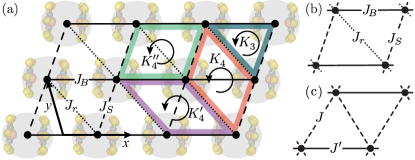
Figure 1: We find three significant antiferromagnetic nearest-neighbor couplings within the layers of [Pd(dmit)₂]₂ dimers (a). The largest, $J_{B}$, is in the dimer stacking direction. The others, $J_{r}\neq J_{S}$ lead to a scalene lattice (b). We show that the physics of this model differs importantly from the isosceles triangular lattice relevant to the closely related BEDT-TTF salts (c). We also calculate the three and four-site ring exchange interactions, $K_{3}$, $K_{4}$, $K^{\prime}_{4}$, and $K^{\prime\prime}_{4}$ (a). The interlayer coupling, $J_{z}$, is approximately perpendicular to the page.

In this work we parametrize the spin model of EtMe3Sb including the scalene Heisenberg and ring exchange interactions using broken symmetry density functional theory (BS-DFT) calculations Assfeld and Rivail (1996); David et al. (2017); Coulaud et al. (2013, 2012). We find that the strongest exchange coupling is along the dimer stacking direction ($J_{B}$; cf. Fig. 1a). We solve our model via the chain random phase approximation (CRPA) around the large $J_{B}$ limit. In this approach, one starts from the exact form for the one-dimensional magnetic susceptibility of a Heisenberg spin-1/2 chain and treats interchain interactions via the RPA Schulz (1996); Bocquet et al. (2001). On an isosceles triangular lattice, the interchain interactions are perfectly frustrated. Within the CRPA, this prevents ordering at any temperature Bocquet et al. (2001); Kenny et al. (2019). In EtMe3Sb, we find that the anisotropy in the interchain coupling leads to an effective unfrustrated interchain interaction, given by the difference of the interchain couplings ($\delta J_{y}=J_{r}\!-\!J_{S}$). This favors long-range order. On the other hand, ring exchange favors quantum disorder Motrunich (2005); Misguich et al. (1998, 1999); Merino et al. (2014); Holt et al. (2014). Combining our BS-DFT and CRPA results shows that the absence of long-range magnetic order in EtMe3Sb springs from the interplay of one-dimensionalization and ring exchange, leading us to propose that the ground state of EtMe3Sb is adiabatically connected to the TLL.

II Parametrization of Spin Model with Broken-Symmetry Density Functional Theory

The low-energy physics of the insulating phase of EtMe3Sb is described by an extended Hubbard model Powell and McKenzie (2011); Kanoda and Kato (2011); Nakamura et al. (2012),

$$\mathcal{H}_{\mathrm{Hubbard}}=\sum_{ij\sigma}t_{ij}c^{\dagger}_{i\sigma}c_{j\sigma}+U\sum_{i}n_{i\uparrow}n_{i\downarrow}+\frac{1}{2}\sum_{i\neq j}\Bigg{[}\left(\sum_{\sigma\rho}V_{ij}^{*}c^{\dagger}_{i\sigma}c^{\dagger}_{j\rho}c_{j\rho}c_{i\sigma}\right)+(J_{ij}^{\mathrm{DE}}+J_{ij}^{\mathrm{SP}}){\bm{S}}_{i}\cdot{\bm{S}}_{j}-\frac{J_{ij}^{\mathrm{DE}}}{2}{c}_{i\uparrow}^{\dagger}{c}_{i\downarrow}^{\dagger}{c}_{j\uparrow}{c}_{j\downarrow}\Bigg{]},$$ (1)

where $c^{\dagger}_{i\sigma}$ ($c_{i\sigma}$) creates (destroys) an electron with spin $\sigma$ on site (dimer) $i$, $t_{ij}$ is the hopping between sites, $U$ is the effective on-site Coulomb repulsion, $n_{i\sigma}=c^{\dagger}_{i\sigma}c_{i\sigma}$ is the electron density, $V_{ij}^{*}=V_{ij}+(J_{ij}^{\mathrm{DE}}/4)$, $V_{ij}$ is the Coulomb repulsion between electrons on different dimers, $J_{ij}^{\mathrm{DE}}$ is the interdimer direct exchange, and $J_{ij}^{\mathrm{SP}}$ is the interdimer spin polarization. While there have been a number of calculations of $t_{ij}$ Scriven and Powell (2012); Jacko et al. (2013); Tsumuraya et al. (2013); Sup , only Nakamura et al. Nakamura et al. (2012) have previously estimated $U$ and $V_{ij}$. They also calculated the direct exchange $J_{ij}^{\mathrm{DE}}$. Although $|J_{ij}^{\mathrm{DE}}|\ll U,V_{ij}$, Nakamura et al.’s parameters show that $J_{ij}^{\mathrm{DE}}$ is non-negligible on the scale of the superexchange interaction, $J_{ij}^{\mathrm{SE}}$ .

We construct an effective low-energy spin model of the Mott insulating phase for $t_{B}\ll U-V_{B}$. As well as the usual superexchange interactions, we also retain the three- and four-site ring exchange, illustrated in Fig. 1a,

$$\mathcal{H}= \frac{J_{B}}{2}\sum_{\leavevmode\hbox to9.03pt{\vbox to3pt{\text{[drawing]}}}}\hat{P}_{ij}+\frac{J_{z}}{2}\sum_{\leavevmode\hbox to10pt{\vbox to9.03pt{\text{[drawing]}}}}\hat{P}_{ij}+\frac{J_{S}}{2}\sum_{\leavevmode\hbox to4.81pt{\vbox to7.82pt{\text{[drawing]}}}}\hat{P}_{ij}+\frac{J_{r}}{2}\sum_{\leavevmode\hbox to7.22pt{\vbox to7.82pt{\text{[drawing]}}}}\hat{P}_{ij}$$

$$+\frac{K_{3}}{2}\sum_{\leavevmode\hbox to9.03pt{\vbox to7.82pt{\text{[drawing]}}}}\left(\hat{P}_{ijk}+\hat{P}_{lkj}\right)+\frac{K_{4}}{2}\sum_{\leavevmode\hbox to9.03pt{\vbox to12.64pt{\text{[drawing]}}}}\left(\hat{P}_{ijkl}+\hat{P}_{lkji}\right)+\frac{K^{\prime}_{4}}{2}\sum_{\leavevmode\hbox to13.25pt{\vbox to7.82pt{\text{[drawing]}}}}\left(\hat{P}_{ijkl}+\hat{P}_{lkji}\right)+\frac{K^{\prime\prime}_{4}}{2}\sum_{\leavevmode\hbox to10.84pt{\vbox to7.82pt{\text{[drawing]}}}}\left(\hat{P}_{ijkl}+\hat{P}_{lkji}\right)$$ (2)

where $J_{ij}^{\mathrm{SE}}=4t_{ij}^{2}/U_{ij}$, $U_{ij}=U-V_{ij}$, $J_{ij}=J_{ij}^{\mathrm{SE}}+J_{ij}^{\mathrm{DE}}+J_{ij}^{\mathrm{SP}}$ [we retain only $\{i,j\}\in\{B,S,r\}$ (cf. Fig. 1a,b)], $K_{3}=3t_{B}t_{r}t_{S}/U_{\textrm{eff}}^{2}$, $K_{4}\!=\!80t_{r}^{2}t_{S}^{2}/U_{\textrm{eff}}^{3}$, $K_{4}^{\prime}\!=\!80t_{r}^{2}t_{B}^{2}/U_{\textrm{eff}}^{3}$, $K_{4}^{\prime\prime}\!=\!80t_{S}^{2}t_{B}^{2}/U_{\textrm{eff}}^{3}$, $U_{\textrm{eff}}\simeq U-\frac{1}{3}(V_{B}+V_{S}+V_{r})$, which is a reasonable approximation as the three $V$’s do not vary greatly, vida infra, $\hat{P}_{ij}\!=\!2\bm{S}_{i}\cdot\bm{S}_{j}+\frac{1}{2}$, $\hat{P}_{ijk}\!=\!\hat{P}_{ij}\hat{P}_{jk}$, $\hat{P}_{ijkl}\!=\!\hat{P}_{ij}\hat{P}_{jk}\hat{P}_{kl}$, and $\hat{P}_{ijk}$ and $\hat{P}_{ijkl}$ cyclically permute spin states around the plaquettes shown (with dashing to match Figs. 1a,b).

Significant effort has been expended parameterizing tight-binding models for EtMe3Sb from DFT Scriven and Powell (2012); Tsumuraya et al. (2013); Jacko et al. (2013); Sup . However, these calculations do not give a direct parameterization of the spin model [Eq. (2)] because they do not enable the calculation of $U$, $V_{ij}$, $J_{ij}^{\mathrm{DE}}$, or $J_{ij}^{\mathrm{SP}}$. Nakamura et al. Nakamura et al. (2012) addressed this by performing constrained RPA calculations, which do provide estimates of the Coulomb interactions. All these calculations are based on pure density functionals, i.e., the local density approximation (LDA) or generalized gradient approximations (GGA), which are known to perform poorly for parametrizing magnetic interactions Malrieu et al. (2014); Moreira et al. (2002); Zein et al. (2009); Phillips and Peralta (2012). In particular, they underestimate $J_{ij}^{\mathrm{SE}}$ Coulaud et al. (2012). For further discussion of functionals, see the Supplementary Material Sup .

LDA+U calculations are not straightforward in these molecular systems; like many inorganic and organometallic magnets, the spins are delocalized over a dimer rather than being centered on a single atom. However, hybrid functionals have been shown to provide similar accuracy as the LDA+U calculations in many molecular systems Malrieu et al. (2014); Rivero et al. (2009).

Previous tight-binding models based on either the monomer or dimer models of EtMe3Sb Scriven and Powell (2012); Tsumuraya et al. (2013); Jacko et al. (2013); Nakamura et al. (2012); Powell and McKenzie (2011) neglect states outside of a small energy window near the Fermi surface. These models are based on Kohn-Sham eigenvalues, which have no formal correspondence to nature but are a device for calculating the total density Kohn and Sham (1965). In practice, Kohn-Sham eigenvalues poorly reproduce energy differences even in weakly correlated materials Jones and Gunnarsson (1989); Perdew (1985) and dramatically fail in strongly correlated materials. For example, in EtMe3Sb, $\kappa$-Cu, and $\kappa$-Ag the Kohn-Sham band structure is metallic Scriven and Powell (2012); Tsumuraya et al. (2013); Jacko et al. (2013); Nakamura et al. (2012); Powell and McKenzie (2011) rather than insulating, as in experiment Powell and McKenzie (2011); Kanoda and Kato (2011).

In BS-DFT, one calculates exchange interactions by comparing total energies of the full atomistic Hamiltonian, which have a formal basis in DFT and are highly accurate in practice. Recent advances David et al. (2017); Coulaud et al. (2013, 2012) have made it possible to isolate distinct physical contributions to the total exchange and even the Hubbard parameters from this approach. Thus, EtMe3Sb provides a valuable opportunity for a comparison of BS-DFT with constrained RPA. BS-DFT calculations are based on a cluster, rather than an infinite crystal. This is a double-edged sword. Finite size effects need to considered, but the finite size makes hybrid functionals, which include exact exchange interactions, computationally tractable.

In light of these considerations, we calculated $J_{ij}^{\mathrm{SE}}$, $J_{ij}^{\mathrm{DE}}$, $J_{ij}^{\mathrm{SP}}$, $t_{ij}$, and $U-V_{ij}$ for each nearest neighbor pair of dimers from a series of BS-DFT calculations. We utilize the frozen orbital capabilities of the local self-consistent field method David et al. (2017); Coulaud et al. (2013, 2012); Assfeld and Rivail (1996). We use the “quasi-restricted” orbital (QRO) approach Neese (2006) with LANDL2DZ effective core potential and basis set for palladium and antimony Hay and Wadt (1985); Wadt and Hay (1985) and 6-31+G* basis set Clark et al. (1983); Ditchfield et al. (1971); Hariharan and Pople (1973); Hehre et al. (1972) for other atoms and with hybrid B3LYP functional Becke (1993) in ORCA Neese (2012). See the Supplementary Material Sup for results with a different amount of Hartree-Fock exchange, which has been shown to have an effect on BS-DFT couplings David et al. (2017); Martin and Illas (1997); Sorkin et al. (2008); Reiher et al. (2001); Swart et al. (2004); Dai et al. (2005); Lawson Daku et al. (2005); Pierloot and Vancoillie (2006); Rong et al. (2006); Brewer et al. (2006); Vargas et al. (2006); Ovcharenko et al. (2007); Valero et al. (2008). We included the six nearest cations to each Pd(dmit)₂ tetramer; benchmarking revealed that the calculated exchange interactions are well converged at this cluster size. We use the experimental crystal structure measured at 4 K Yug .

As illustrated in Fig 2, we start with a triplet state in the quasi-restricted open-shell formalism (T,QRO). We split the high spin dimer one-electron orbitals into two different sets, (i) the two same spin localized magnetic orbitals and (ii) the remaining (non-magnetic) ones. A BS solution is found by flipping the individual spin state of one magnetic orbital (BS,QRO in Fig 2), giving us the direct exchange, $J_{ij}^{\mathrm{DE}}$. We then relax (i.e. delocalize) only the magnetic orbitals in the BS solution (BS,UFC in Fig 2), which allows us to calculate the superexchange $J_{ij}^{\mathrm{SE}}$ and the Hubbard parameters $t_{ij}$ and $U-V_{ij}$, as described in David et al. (2017). The magnetic orbitals are then kept frozen in both the triplet and BS states while the non-magnetic ones are relaxed (T,UFM and BS,UFM in Fig 2), eventually giving the spin-polarization contribution, $J_{ij}^{\mathrm{SP}}$.

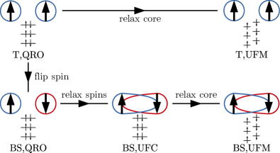
Figure 2: Illustration of the decomposition of the magnetic exchange coupling calculation. Blue and red circles represent magnetic orbitals (singly) occupied by spin-up and spin-down electrons respectively. Horizontal black lines and vertical arrows represent non-magnetic occupied orbitals (also known as core orbitals).

Our BS-DFT results are shown in Table 1. We calculate small values for the spin-polarisation contribution, $J^{\mathrm{SP}}\sim 0.05J_{B}$, and henceforth neglect this term. The unfrustrated interlayer coupling is $J_{z}=0.06$ K.

Our values for the total Heisenberg exchange ($J_{ij}$) between dimers reveal that the exchange along the dimer stacking direction, $J_{B}$ (see Fig. 1a), is significantly larger than the others; $J_{r}/J_{B}=0.35$ and $J_{S}/J_{B}=0.30$. In what follows, it will be convenient to make a change of variables to the average of the interchain couplings, $\bar{J_{y}}=\frac{1}{2}\left(J_{S}\!+\!J_{r}\right)\!=\!135$ K, and their difference, $\delta J_{y}=J_{r}\!-\!J_{S}\!=\!22$ K.

$ij$	$J_{ij}$ (K)	$J_{ij}^{\mathrm{SE}}$ (K)	$J_{ij}^{\mathrm{DE}}$ (K)	$t_{ij}$ (meV)	$U\!-\!V_{ij}$ (meV)
B	414	481	-67	80	565
r	146	168	-22	47	600
S	124	168	-44	44	519

Table 1: Calculated nearest neighbour interactions between dimers of EtMe3Sb, as shown in Figure 1a. The full Heisenberg exchange ($J_{ij}$) is a sum of the superexchange ($J_{\mathrm{SE}}$) and the direct exchange ($J_{\mathrm{DE}}$). $t_{ij}$ is the effective hopping between dimers and $U\!-\!V_{ij}$ is the effective Coulomb interaction on each dimer.

In the limit $\delta J_{y}$ and $J_{z}\rightarrow 0$, the lattice becomes a quasi-one-dimensional isosceles model (cf. Fig. 1c). Numerical studies have shown that this model remains quasi-one-dimensional for $\bar{J_{y}}/J_{B}<0.7$ Weng et al. (2006); Yunoki and Sorella (2006); Hayashi and Ogata (2007); Pardini and Singh (2008); Jiang et al. (2009); Heidarian et al. (2009); Tay and Motrunich (2010). The unfrustrated limit (explored by Schulz Schulz (1996)) occurs when $J_{S}\rightarrow 0$ or $J_{r}\rightarrow 0$, in which case the magnitude of the unfrustrated interchain coupling is $|\delta J_{y}|$. This model is quasi-one-dimensional for $(|\delta J_{y}|\!+\!|J_{z}|)/J_{B}<0.3$ Yasuda et al. (2005). In EtMe3Sb, both the frustrated component of the interchain coupling, $\bar{J_{y}}/J_{B}\!=\!0.33\ll 0.7$, and the total unfrustrated component, $\left(|\delta J_{y}|\!+\!|J_{z}|\right)/J_{B}\!=\!0.05\ll 0.3$, are comfortably within quasi-one-dimensional limits.

We determine the ring exchange parameters (cf. Eq. 2) using our values of $t_{ij}$ and $U\!-\!V_{ij}$. The three-site ring exchange, $K_{3}\!=\!18$ K, simply renormalizes the Heisenberg couplings within the Pd(dmit)₂ planes; $J_{B}\rightarrow J_{B}\!+\!K_{3}$ and $\bar{J_{y}}\rightarrow\bar{J_{y}}\!+\!K_{3}$ Misguich et al. (1998). The four-site terms are slightly larger: $K_{4}\!=\!23$ K, $K_{4}^{\prime}\!=\!76$ K, $K_{4}^{\prime\prime}\!=\!66$ K. These terms are also more consequential due to effective interactions in additional directions within the lattice. To include them in an effective Heisenberg model, we use a leading order mean-field approximation Holt et al. (2014), $\langle\bm{S}_{\alpha}\cdot\bm{S}_{\beta}\rangle=S^{2}\cos(\bm{k}\cdot\bm{r}_{\alpha\beta})$, where $\bm{r}_{\alpha\beta}$ is the vector from site $\alpha$ to site $\beta$. This results in renormalised exchange couplings $J_{ij}$ in the $\bm{x}$, $\pm\frac{1}{2}\bm{x}-\bm{y}$, $\pm\frac{3}{2}\bm{x}-\bm{y}$, and $2\bm{y}$ directions (see axes in Fig. 1a).

III EtMe₃Sb as a Quasi-1D Spin System

III.1 Néel Ordering Temperature

The Néel ordering temperature, $T_{N}$, of a lattice of weakly coupled chains can be calculated using the CRPA expression for the three-dimensional dynamical magnetic susceptibility, Scalapino et al. (1975); Schulz (1996); Essler et al. (1997); Bocquet et al. (2001)

$$\chi\left(\omega,\bm{k},t\right)=\frac{\chi_{\mathrm{chain}}(\omega,k_{x},t)}{1-2\tilde{J}_{\perp}\left(\bm{k}\right)\chi_{\mathrm{chain}}(\omega,k_{x},t)},$$ (3)

where $t\!=\!k_{B}T/(J_{B}+K_{3})$ is the reduced temperature, $\tilde{J}_{\perp}(\bm{k})$ is the Fourier transform of the interchain coupling and $\bm{k}\!=\!\left(k_{x},k_{y},k_{z}\right)$ is the crystal momentum along the axes in Fig. 1a in units of the inverse lattice spacing. The dynamical susceptibility for a single Heisenberg chain, calculated from a combination of the Bethe ansatz and field theory techniques, is Bethe (1931); Schulz and Bourbannais (1983); Schulz (1986); Barzykin (2000); Tsvelik (2003)

$$\chi_{\mathrm{chain}}(\omega,k_{0},t)=-\frac{\sqrt{\ln({\Lambda}/{t})}}{2t(2\pi)^{3/2}}\frac{\Gamma\left(\frac{1}{4}-i\frac{\omega-uk_{0}}{4\pi t}\right)}{\Gamma\left(\frac{3}{4}-i\frac{\omega-uk_{0}}{4\pi t}\right)}\frac{\Gamma\left(\frac{1}{4}-i\frac{\omega+uk_{0}}{4\pi t}\right)}{\Gamma\left(\frac{3}{4}-i\frac{\omega+uk_{0}}{4\pi t}\right)},$$ (4)

where $k_{0}=k_{x}-\pi$, $\Gamma(x)$ is the Euler gamma function, $u=\frac{\pi}{2}J_{x}b_{0}$ is the spin velocity, $b_{0}$ is the interdimer separation along the quasi-one-dimensional stack, and $\Lambda\simeq 24.27$ Barzykin (2001). The Néel temperature, $T_{N}$, corresponds to the zero frequency pole in $\chi\left(\omega,\bm{k},t\right)$ when $2\tilde{J}_{\perp}\left(\bm{k}\right)\chi_{\mathrm{chain}}(0,k_{x})|_{T=T_{N}}=1$. The instability occurs at the maximum of $J_{\perp}\left(\bm{k}\right)\chi_{\mathrm{chain}}(0,k_{x})$.

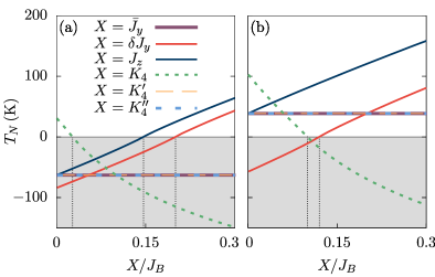
Figure 3: Numerical calculation of the ordering temperature as a function of each parameter in Eq. (2). Each line corresponds to varying one parameter, $X$, and keeping the others constant. In (a), all parameters (except for $X$) are set to our values for EtMe3Sb. In this case, solutions for $T_{N}$ are only positive when $K_{4}$ is very small or $\delta J_{y}$, $J_{z}$ are large. Solutions for $T_{N}$ become negative and complex when $2K_{4}>|\delta J_{y}|+|J_{z}|$ (for these unphysical solutions only the real part is shown). The vertical black lines indicate the parameter values for which this transition occurs. In (b), we set $K_{4}=0.06J_{B}$ and $\delta J_{y}=0.2J_{B}$ as an example of the regime $2K_{4}<|\delta J_{y}|+|J_{z}|$. In both cases, the solution is exactly reproduced with Eq. (5); it is independent of the magnitudes of $\bar{J_{y}}$, $K_{4}^{\prime}$, and $K_{4}^{\prime\prime}$

Numerical exploration of our system (see Fig. 3) reveals that $T_{N}$ is affected only negligibly by $J_{y}$, $K^{\prime}$, $K^{\prime\prime}$, but significantly by $\delta J_{y}$, $J_{z}$, $K_{4}$. We find positive, real solutions only when $2K_{4}<|\delta J_{y}|+|J_{z}|$. We also find, analytically, that only the magnitudes (and not the signs) of each interaction affect $T_{N}$. In light of this, Fig. 4 shows a numerical calculation of $T_{N}$ as a function of the unfrustrated couplings and $K_{4}$. In the gray regions of Figs. 3 and 4, where $2K_{4}<|\delta J_{y}|+|J_{z}|$, there is no real positive solution. This implies that there is no long-range magnetic order, and that this state is in the same phase as the TLL.

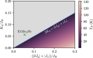
Figure 4: Numerical calculation of the ordering temperature as a function of the interchain ring exchange, $K_{4}$, and the unfrustrated interchain couplings, $\delta J_{y}$ and $J_{z}$. Our calculated parameters for EtMe3Sb are marked by the green cross. We have used our calculated values for the other couplings in Eq. (2); $\bar{J}_{y}\!=\!135$ K, $K_{3}=18$ K, $K^{\prime}_{4}\!=\!76$ K, and $K^{\prime\prime}_{4}\!=\!66$ K. The gray area indicates where there is no real positive solution for $T_{N}$. This occurs when $2K_{4}>|\delta J_{y}|+|J_{z}|$ (as shown with the blue dashed line). For all points on this graph, $k_{0}$ and $k_{y}+\pi/2$ are both less than $10^{-4}$.

For all points in Fig. 4 (including the gray zone) we find $k_{0}\approx 0$ and $k_{y}\approx-\pi/2$. Taking the limits $k_{0}\rightarrow 0$ and $k_{y}\rightarrow-\pi/2$ analytically leads to

$$\frac{T_{N}}{J_{B}}=0.556\frac{|\delta J_{y}|+|J_{z}|-2K_{4}}{J_{B}+3K_{4}}\sqrt{\log\left(\frac{\Lambda}{T_{N}}\right)}.$$ (5)

Thus, for $K_{4}=0$ one finds that $T_{N}\sim|\delta J_{y}|+|J_{z}|$. This agrees precisely with the prediction for a cuboidal model with chains along the $x$-axis coupled by bipartite exchange interactions $\delta J_{y}$, along the $y$-axis and $J_{z}$ along the $z$-axis Schulz (1996). We find that Figs. 3 and 4 are perfectly reproduced by Eq. (5), confirming the relevance of this limit. Thus, we deduce three things: $\bar{J}_{y}$ is the frustrated part of the in-plane interchain interaction, which does not lead to long-range magnetic order and has no influence on $T_{N}$ (for $\delta J_{y}\neq 0$). $\delta J_{y}$ is the unfrustrated part of the in-plane interchain interaction, which can drive a magnetic instability and has a strong influence on $T_{N}$. $K_{4}\neq 0$ strongly suppresses magnetic order (as $K_{4}\propto t_{r}^{2}t_{S}^{2}$ and therefore cannot be negative).

Our DFT parameterization yields $2K_{4}=46$ K, which is greater than our value for $|\delta J_{y}|+|J_{z}|=21$ K. The solution to Eq. 5 for EtMe3Sb is then unphysical; our quasi-1D model, with four-membered ring exchange, predicts that EtMe3Sb will not order magnetically down to $T=0$. This agrees with experiments, where ordering is not detected down to 19.4 mK Itou et al. (2010).

III.2 Experimental Predictions

In light of our findings, we propose that the ‘spin-liquid’ behaviour in EtMe3Sb is a remnant of the TLL found in an isolated chain, similar to the state observed above $T_{N}=0.6$ K in Cs₂CuCl₄ Kohno et al. (2014); Coldea et al. (1997). This provides a natural explanation for the observed low temperature behaviour in EtMe3Sb. The heat capacity Yamashita et al. (2011) reveals gapless excitiations from the ground state. This is consistent with the gapless spinon excitations expected in a TLL Giamarchi (2003). The ¹³C nuclear spin-lattice relaxation rate shows a peak at 1 K Itou et al. (2010). We propose that this could be explained by short range correlations caused by the unfrustrated couplings ($\delta J_{y}$ and $J_{z}$). This could also explain the broad hump in the heat capacity around 3.7 K Yamashita et al. (2011).

Measurements of the thermal conductivity, $\kappa$, of EtMe3Sb have produced conflicting results. Yamashita et al. Yamashita et al. (2010) observe a large residual linear term, attributing this to highly mobile gapless excitations. However, recent studies Bourgeois-Hope et al. (2019); Ni et al. (2019), find no significant residual linear term as $T\rightarrow 0$ and a much lower value for the thermal conductivity. Yamashita has since published a note Yamashita (2019) showing that they observed both types of behaviour for different samples in their experiment, and proposing that the discrepancy is caused by impurities. However, Bourgeois-Hope et al. Bourgeois-Hope et al. (2019) rejected this explanation.

In a quasi-1D system, the thermal conductivity is highly dependent on the lattice direction along which it is measured. This is evident in thermal conductivity measurements on Cs2CuCl4 Schulze et al. (2019). In the spin liquid phase of Cs2CuCl4, a linear contribution, presumably from spinons, is observed in the thermal conductivity along the chain direction, but not along the other crystal axes.

This makes sense if we assume that both spinons and phonons can transport heat along the spin chains, but that only phonons can transfer heat between the chains. Therefore, if the heat transport has a significant interchain component the thermal resistance adds in series, $1/\kappa_{\mathrm{total}}\sim 1/\kappa_{\mathrm{ph}}+1/\kappa_{\mathrm{sp}}$, where $\kappa_{\mathrm{total}}$, $\kappa_{\mathrm{ph}}$, and $\kappa_{\mathrm{sp}}$ are the total, phonon, and spinon thermal conductivities respectively. This leads to a vanishing thermal conductivity $\kappa_{\mathrm{total}}\rightarrow 0$ as $\kappa_{\mathrm{ph}}\rightarrow 0$ when $T\rightarrow 0$. When the thermal conductivity is measured in the direction of the chains, the spinons and phonons are parallel channels and $\kappa_{\mathrm{total}}\sim\kappa_{\mathrm{ph}}+\kappa_{\mathrm{sp}}$. This leads to two important differences from the series transport scenario: (i) the thermal conductivity should be much larger along the chain directions and (ii) there is a residual linear term as $T\rightarrow 0$ because $\kappa_{\mathrm{sp}}/T\neq 0$ only for heat transport parallel to the chains. Thus, a prediction of our theory is that there is a linear term, due to spinons, in the thermal conductivity along the chain direction, which alternates between $[1,1,0]$ and $[1,\bar{1},0]$ in different Pd(dmit)2 layers.

The direction of thermal transport within the Pd(dmit)2 planes is not known in most thermal conductivity measurements in EtMe3Sb to date. Where the direction has been determined Bourgeois-Hope et al. (2019), the heat has always been transported along a crystallographic axis and results in a small thermal conductivity with no linear term – consistent with our predictions (as this corresponds to the series case). Therefore, all data to date is consistent with our theory. Measurements of thermal conductivity along the $[1,1,0]$ or $[1,\bar{1},0]$ directions would be an important test of our theory as they provide the opportunity to falsify it.

III.3 Comparison to Previous First-Principles Studies

It is important to compare our BS-DFT results with other first principles approaches to EtMe3Sb. The in-plane hopping integrals found by Nakamura et al. Nakamura et al. (2012) are within the range found from other parametrizations through band structure calculations Scriven and Powell (2012); Tsumuraya et al. (2013); Jacko et al. (2013). These studies parametrized monomer or dimer tight-binding models on the basis of band structure calculations; either by fitting to models or via Wannier functions. This approach yields tight-binding models with less anisotropy than our BS-DFT, as summarized in Table 2, and very weak hopping between the layers Tsumuraya et al. (2013). The values in Table 2 all lie in or close to the weakly coupled chain regime ($\bar{J}_{y}^{\mathrm{SE}}/J_{B}^{\mathrm{SE}}\lesssim 0.7$; $\delta{J}^{\mathrm{SE}}/J_{B}^{\mathrm{SE}}\lesssim 0.3$).

Ref.	$t_{B}$ (meV)	$t_{r}$ (meV)	$t_{S}$ (meV)	$\bar{J}_{y}^{\mathrm{SE}}/J_{B}^{\mathrm{SE}}$	$\delta{J}^{\mathrm{SE}}/J_{B}^{\mathrm{SE}}$
Nakamura et al. (2012)	54	40	45	0.62	0.14
Jacko et al. (2013)	57	40	47	0.59	0.19
Tsumuraya et al. (2013)	49	42	37	0.65	0.16
Scriven and Powell (2012)	49	38	46	0.74	0.28

Table 2: Previous results for inter-dimer hoppings based on DFT band-structure calculations. To estimate the ratio of exchange couplings, we use the superexchange in the large $U$ limit, $\bar{J}_{y}^{\mathrm{SE}}\approx\frac{4}{U}\frac{t_{S}^{2}+t_{r}^{2}}{2}$, $\delta J_{y}\approx\frac{4}{U}(t_{S}^{2}+t_{r}^{2})$ and $J_{B}^{\mathrm{SE}}\approx 4t_{B}^{2}/U$, which leads to $J_{B}^{\mathrm{SE}}/\bar{J}_{y}^{\mathrm{SE}}\sim 2t_{B}^{2}/(t_{r}^{2}+t_{S}^{2})$. All of these models lie in or close to a weakly coupled chain regime ($\bar{J}_{y}^{\mathrm{SE}}/J_{B}^{\mathrm{SE}}\lesssim 0.7$; $\delta{J}^{\mathrm{SE}}/J_{B}^{\mathrm{SE}}\lesssim 0.3$) which gives rise to a gapless spin-liquid state Weihong et al. (1999); Fjærestad et al. (2007); Yunoki and Sorella (2006); Hayashi and Ogata (2007); Tocchio et al. (2014); Ghorbani et al. (2016).

Furthermore, Nakamura et al.’s constrained RPA calculations of the Coulomb interactions allow for a fairly direct comparison with our BS-DFT results. We find that our values for $U\!-\!V_{ij}$ are similar in magnitude, following the same trend, and we also find a similar correlation strength, $U/t_{B}\approx 7$. In our notation, Nakamura et al. found that $J_{B}=262$ K, $\bar{J}_{y}=157$ K, $\delta{J_{y}}=47$ K, and $K_{4}=43$ K. As $\bar{J}_{y}/J_{B}=0.60<0.7$ and $\delta{J_{y}}/J_{B}=0.18<0.3$ the CRPA approach should still be reasonable, although Nakamura et al.’s values are less quasi-one-dimensional than those found in our BS-DFT calculations. We have performed BS-DFT calculations using pure funtionals (LDA and PBE) and find that these provide a poor description of EtMe3Sb, as witnessed by a large spin contamination. This may explain the discrepancy. Furthermore, BS-DFT calculations are differences of total energies, whereas band structure calculations are based on Kohn-Sham eigenvalues. The former are far more accurate in DFT. Regarding the interlayer hopping integral, Nakamura et al. do not report a value, but similar calculations by Tsumuraya et al. find that there is very weak hopping between the layers Tsumuraya et al. (2013). Thus it is safe to assume that $J_{z}<18$ K. Whence, $2K_{4}>|\delta J_{y}|\!+\!|J_{z}|$ and Nakamura et al.’s parameters also place EtMe3Sb in the quantum disordered regime. Moreover, a recalculation of Fig. 4 with Nakamura et al’s values for $\bar{J_{y}}$, $K_{4}^{\prime}$, and $K_{4}^{\prime\prime}$ (see the Supplementary Material Sup ), is a reproduction of Fig. 4 because $T_{N}$ depends only on $\delta J_{y}$, $J_{z}$, and $K_{4}$.

The quasi-one-dimensionality of the spin Hamiltonian derived from band structure calculations has been previously noted Nakamura et al. (2012); Tsumuraya et al. (2013), although detailed many-body calculations have not previously been performed in this regime of the scalene triangular lattice.

IV Conclusions

We have used an atomistic approach to parametrize an extended Hubbard model, and thence a spin model, for the spin-liquid candidate EtMe3Sb. This revealed a frustrated scalene triangular lattice where the largest coupling along the stacking direction is nearly three times larger than the others. We showed that, in the quasi-one-dimensional limit relevant to EtMe3Sb, the difference in the interchain coupling acts identically to an unfrustrated interchain coupling and favors long-range magnetic order. This interaction competes with ring exchange, which promotes quantum disorder. Our DFT calculations show that, in EtMe3Sb, $2K_{4}>|\delta J|+|J_{z}|$ and we therefore predict that EtMe3Sb does not order magnetically even at $T=0$. Thus, we propose that the ‘spin-liquid’ behaviour is a remnant of TLL behavior in weakly coupled 1D spin chains.

We predict that thermal transport along the chains is very different from that with a significant transverse component. This is because in the former case spinons and phonons act as parallel channels whereas in the latter they transport heat in series. This means (i) that the thermal conductivity along the chains is much larger than the thermal conductivity across the chains and (ii) that there is a large linear contribution to the thermal conductivity along the chains (due to the spinons), but no linear contribution to transverse thermal conductivity. Behaviours consistent with both the parallel and series pictures have been observed experimentally, resulting in some controversy. Where the thermal transport direction is know it is along crystallographic axes and consistent with our predictions for series heat transport. Measurements of heat transport along the chains (in the $[1,1,0]$ and $[1,\bar{1},0]$ directions) would provide a key test of our theory and could either confirm or falsify it.

Supplementary Material

CRPA analysis using Hamiltonian parameters from Nakamura et al.

Nakamura et al. Nakamura et al. (2012) previously parametrized the extended Hubbard model for EtMe3Sb using the constrained random-phase approximation (RPA) and maximally localized Wannier orbitals. Their values are shown in Table 3, which lead to $K_{4}=43$ K, $K_{4}^{\prime}=63$ K, and $K_{4}^{\prime\prime}=78$ K. Fig. 5 is equivalent to Fig. 4 in the main text, but it is based on their values. We find that their parametrization leads to the same prediction that ring exchange overcomes the unfrustrated couplings and causes spin disorder, since $2K_{4}>|\delta J_{y}|$. Note that Nakamura et al. Nakamura et al. (2012) did not calculate an inter-layer coupling, $J_{z}$, but another study using similar methods finds very weak hopping between the layers Tsumuraya et al. (2013).

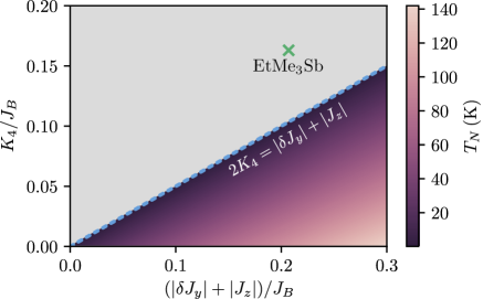
Figure 5: A recalculation of Fig. 4 in the main text with Nakamura et al’s Nakamura et al. (2012) values for $\bar{J_{y}}$, $K_{4}^{\prime}$, and $K_{4}^{\prime\prime}$ (shown in Table 3). The green cross indicates their values for $K_{4}$ and $\delta J_{y}$, which lie in the disordered regime. It is otherwise indistinguishable from Fig. 4 because $T_{N}$ depends only on $\delta J_{y}$, $J_{z}$, and $K_{4}$.

$ij$	$J_{ij}$ (K)	$J_{ij}^{\mathrm{SE}}$ (K)	$J_{ij}^{\mathrm{DE}}$ (K)	$t_{ij}$ (meV)	$U\!-\!V_{ij}$ (meV)
B	262	335	-73	54	410
r	133	170	-37	40	440
S	180	240	-60	45	390

Table 3: Nearest neighbour interactions between dimers of EtMe3Sb calculated by Nakamura et al. Nakamura et al. (2012). Labels as shown in Figure 1a of the main text. The full Heisenberg exchange ($J_{ij}$) is a sum of the superexchange ($J_{\mathrm{SE}}$) and the direct exchange ($J_{\mathrm{DE}}$). $t_{ij}$ is the effective hopping between dimers and $U\!-\!V_{ij}$ is the effective Coulomb interaction on each dimer.

Effect of DFT functional on BS-DFT coupling parameters

The magnetic exchange coupling calculated with broken-symmetry density functional theory (BS-DFT) is strongly dependent on the amount of Hartree-Fock exchange (%HFX) used within the chosen functional. This feature has been widely studied in the molecular magnet framework Martin and Illas (1997); Sorkin et al. (2008); Reiher et al. (2001); Swart et al. (2004); Dai et al. (2005); Lawson Daku et al. (2005); Pierloot and Vancoillie (2006); Rong et al. (2006); Brewer et al. (2006); Vargas et al. (2006); Ovcharenko et al. (2007); Valero et al. (2008) and its influence on the model Hamiltonian parameters (Heisenberg and Hubbard) investigated by some of the authors David et al. (2017). Table 4 shows a comparison of some Hamiltonian parameters (c.f. Table 1 in the manuscript) calculated using B3LYP with 20 and 50%HFX. In the manuscript, we used the original B3LYP, which has 20%HFX. As shown in the table 4 this variation mainly affects the Hubbard $U$ parameter, which evolves proportionally with the amount of HFX. Indeed increasing the amount of HFX tends to reduce the self interaction error yielding molecular orbitals less delocalized. Therefore the on-site repulsion energy $U$ becomes more important. The kinetic exchange contribution $J_{ij}^{\mathrm{SE}}$, being proportional to $1/U$, is dramatically reduced for the amount of HFX going from 20% to 50%. Therefore the total magnetic coupling $J_{ij}$ appears weaker for 50%HFX than 20%HFX.

	$ij=$r		$ij=$S
	20%HFX	50%HFX	20%HFX	50%HFX
$J_{ij}$ (K)	146	38	124	52
$J_{ij}^{\mathrm{SE}}$ (K)	168	53	168	101
$J_{ij}^{\mathrm{DE}}$ (K)	-22	-15	-44	-49
$t_{ij}$ (meV)	47	43	44	54
$U\!-\!V_{ij}$ (meV)	600	1627	519	1326

Table 4: Comparison of BS-DFT results using B3LYP with 20% HFX and 50% HFX.