Efficient Multi-Agent Trajectory Planning with Feasibility Guarantee using Relative Bernstein Polynomial

Abstract

This paper presents a new efficient algorithm which guarantees a solution for a class of multi-agent trajectory planning problems in obstacle-dense environments. Our algorithm combines the advantages of both grid-based and optimization-based approaches, and generates safe, dynamically feasible trajectories without suffering from an erroneous optimization setup such as imposing infeasible collision constraints. We adopt a sequential optimization method with dummy agents to improve the scalability of the algorithm, and utilize the convex hull property of Bernstein and relative Bernstein polynomial to replace non-convex collision avoidance constraints to convex ones. The proposed method can compute the trajectory for 64 agents on average 6.36 seconds with Intel Core i7-7700 @ 3.60GHz CPU and 16G RAM, and it reduces more than $50\%$ of the objective cost compared to our previous work. We validate the proposed algorithm through simulation and flight tests.

I INTRODUCTION

Multi-agent systems with many unmanned aerial vehicles (UAVs) broaden the range of achievable missions to complex environments unsafe or hard to reach for humans or a single agent. For successful operation of these multi-agent systems, path planning algorithm is required to generate a collision-free trajectory in any obstacle environment. However, many works have a risk to fail in dense cluttered environments due to deadlock [1, 2] or failure caused by enforcing infeasible collision constraints in the formulation [3, 4].

In this paper, we present an efficient multi-agent trajectory planning algorithm which generates safe, dynamically feasible trajectories in obstacle-dense environments by extending our previous work [5]. The proposed algorithm is designed to have the advantages of both grid-based and optimization-based approaches. First, it guarantees the feasibility of optimization problem formulation by utilizing an initial trajectory computed from grid-based multi-agent path finding algorithm. Second, it generates a continuous dynamically feasible trajectory by optimizing the initial trajectory with consideration of quadrotor dynamics as shown in Fig. 1. When we formulate the optimization problem, we utilize the convex hull property of relative Bernstein polynomial to translate non-convex collision avoidance constraints to convex ones. Compared to the previous work [5], we modify the method for constructing constraints not to occur infeasible constraints between collision avoidance constraints, and we introduce a sequential optimization method. This sequential method can deal with a large scale of agents with improved computational efficiency, and does not cause deadlock by employing dummy agents.

Our main contributions can be summarized as follows.

• A multi-agent trajectory planning algorithm is presented for obstacle-dense environments, which generates collision-free and dynamically feasible trajectories without a potential optimization failure by using relative Bernstein polynomial.

• A sequential trajectory optimization method is proposed with dummy agents, which reduces computational load.

• The source code will be released in https://github.com/qwerty35/swarm_simulator.

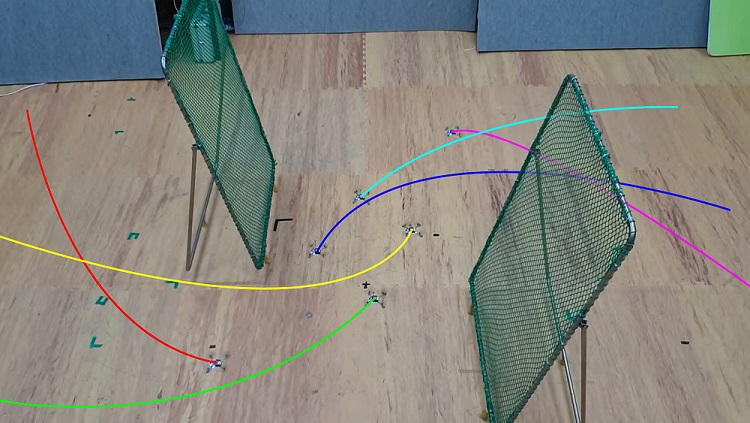
Figure 1: Flight in an obstacle environment with 6 quadrotors.

There have been discussions in literature closely related to our work on multi-agent trajectory planning. In [6, 7, 3], the trajectory generation problems are reformulated as mixed-integer quadratic programming (MIQP) or sequential convex programming (SCP) problems, that apply collision constraints at each discrete time step. These methods suit well systems with a small number of agents, but they are intractable for large teams and complex environments because an additional adaptation process is required to find proper discretization time step depending on the size of agents and obstacles. On the other hand our method does not require this process because we do not use time discretization.

Sequential planning proposed in [8] for better scalability is similar to our work. However, it may not be able to find a feasible solution for a crowded situation. To solve this, we adopt dummy agents which move along the initial trajectory computed by a grid-based planner to prevent deadlock. The most relevant work can be found in [9, 10]. They plan an initial trajectory with a grid-based planner and then construct a safe flight corridor (SFC), which indicates a safe region of each agent. However, they need to resize SFC iteratively until the overall cost converges, while our proposed method does not need an additional resizing process by using relative Bernstein polynomial.

Recently, distributed planning is receiving much attention due to scalability [1, 2, 4]. However, such distributed methods are not able to guarantee a safe solution in obstacle-dense environments due to deadlock.

II PROBLEM FORMULATION

In this section, we formulate an optimization problem to generate safe, continuous trajectories for a multi-agent robot system consisting of $N$ quadrotors. We assign the mission for the $i^{th}$ quadrotor to move from the start point $s^{i}$ to the goal point $g^{i}$. The quadrotors may have a different size with radius $r^{1},...,r^{N}$m. The maximum velocity and acceleration of the $i^{th}$ quadrotor are $v^{i}_{max}$, $a^{i}_{max}$ respectively.

II-A Assumption

We assume that prior knowledge of the free space $\mathcal{F}$ of the environment is given as a 3D occupancy map. We also assume that the grid-based initial trajectory planner in section V-A can find a solution when the grid size is $d$.

II-B Trajectory Representation

Due to the differential flatness of quadrotor dynamics, it is known that the trajectory of quadrotor can be represented in a polynomial function with flat outputs in time $t$ [11]. However, it is difficult to handle collision avoidance constraints with standard polynomial basis. For this reason, we formulate the trajectory of quadrotors using a piecewise Bernstein polynomial. The Bernstein polynomial is the linear combination of Bernstein basis polynomials, and the Bernstein basis polynomial of degree $n$ is defined as follows:

$$B_{k,n}(t)={n\choose k}t^{k}(1-t)^{n-k}$$ (1)

for $t\in[0,1]$ and $k=0,1,...,n$. The trajectory of the $i^{th}$ quadrotor, $p^{i}(t)\in\mathbb{R}^{3}$, can be represented as $M$-segment piecewise Bernstein polynomials:

$$p^{i}(t)=\begin{cases}\ \sum_{k=0}^{n}c^{i}_{1,k}B_{k,n}(\tau_{1})&t\in[T_{0},T_{1}]\\ \ \sum_{k=0}^{n}c^{i}_{2,k}B_{k,n}(\tau_{2})&t\in[T_{1},T_{2}]\\ \ \mathmakebox[\widthof{{}={}}][c]{\vdots}&\mathmakebox[\widthof{{}\in{}}][c]{\vdots}\\ \ \sum_{k=0}^{n}c^{i}_{M,k}B_{k,n}(\tau_{M})&t\in[T_{M-1},T_{M}]\\ \end{cases}$$ (2)

where $\tau_{m}=\frac{t-T_{m-1}}{T_{m}-T_{m-1}}$, $c^{i}_{m,k}$ is the $k^{th}$ control point of the $m^{th}$ segment of the $i^{th}$ quadrotor’s trajectory, and $T_{m-1},T_{m}$ are the start and end time of the $m^{th}$ segment, respectively. Thus, the decision vector of our optimization problem, $c$, consists of all the control points of $p^{i}(t)$ for $i=1,...,N$.

II-C Objective Function

We define the objective function to minimize the integral of the square of the $\phi^{th}$ derivative:

$$J=\sum\limits_{i=1}^{N}\int_{T_{0}}^{T_{M}}\left\|\frac{d^{\phi}}{dt^{\phi}}p^{i}(t)\right\|^{2}_{2}dt=c^{T}Qc$$ (3)

where $Q$ is the Hessian matrix of the objective function. In this paper, we set $\phi=3$ to minimize the jerk of the trajectory, so that the input to the quadrotor becomes less aggressive [12].

II-D Convex Constraints

The trajectory must pass the start and goal points and should be continuous up to the $\phi-1^{th}$ derivatives. Also, it must not exceed maximum velocity and acceleration. These constraints can be written in affine equality and inequality constraints respectively:

$$A_{eq}c=b_{eq}$$ (4)

$$A_{dyn}c\preceq b_{dyn}$$ (5)

II-E Non-Convex Collision Avoidance Constraints

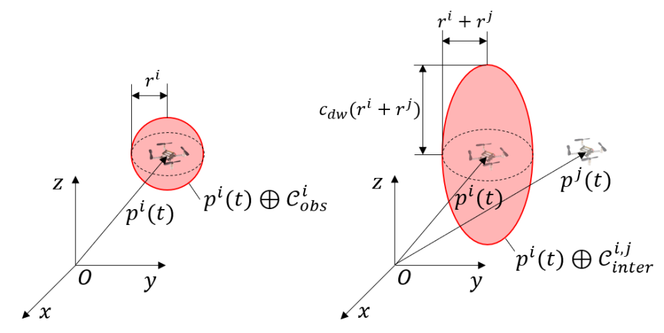
Figure 2: (Left) Obstacle collision model, (Right) Inter-collision model.

II-E1 Obstacle Avoidance Constraints

We define an obstacle collision model of the $i^{th}$ quadrotor, which models a collision region between a quadrotor and obstacles (See Fig. 2):

$$\mathcal{C}^{i}_{obs}=\{p\in\mathbb{R}^{3}\mid\|p\|^{2}_{2}\leq(r^{i})^{2}\}$$ (6)

The $i^{th}$ quadrotor must satisfy the condition below not to collide with obstacles:

$$p^{i}(t)\oplus\mathcal{C}^{i}_{obs}\subset\mathcal{F},\>\>\>\>\>t\in[T_{0},T_{M}]$$ (7)

where $\oplus$ is the Minkowski sum.

II-E2 Inter-Collision Avoidance Constraints

A collision region between $i^{th}$ and $j^{th}$ agents can be expressed with an inter-collision model $\mathcal{C}^{i,j}_{inter}$:

$$\mathcal{C}^{i,j}_{inter}=\{p\in\mathbb{R}^{3}\mid p^{T}Ep\leq(r^{i}+r^{j})^{2}\}$$ (8)

where $E$ is $diag([1,1,1/(c_{dw})^{2}])$, and $c_{dw}$ is a coefficient to consider a downwash effect. The $i^{th}$ agent does not collide with the $j^{th}$ agent if the relative trajectory of the $j^{th}$ agent respect to the $i^{th}$ agent, $p^{i,j}(t)=p^{j}(t)-p^{i}(t)$, satisfies the following condition:

$$p^{i,j}(t)\cap\mathcal{C}^{i,j}_{inter}=\emptyset,\>\>\>\>\>t\in[T_{0},T_{M}]$$ (9)

Non-convexity of (7) and (9) makes it difficult to directly employ them. In the next section, we will show the method that relaxes those non-convex constraints to convex ones using relative Bernstein polynomial.

III Relative Bernstein Polynomial

One of the useful properties of the Bernstein polynomial is a convex hull property that the Bernstein polynomial is confined within the convex hull of its control points [13]. This property has been used to confine the trajectory to a convex set called safe flight corridor (SFC) for obstacle avoidance [14, 15]. Here, we introduce the method to confine the relative polynomial trajectory to inter-collision-free region by utilizing the convex hull property.

Let the $m^{th}$ segment of $p^{i}(t),p^{j}(t)$ be $p^{i}_{m}(t),p^{j}_{m}(t)$ respectively, and $p^{i,j}_{m}(t)=p^{j}_{m}(t)-p^{i}_{m}(t)$ is their relative trajectory. Then $p^{i,j}_{m}(t)$ can be written as

$$\begin{split}p^{i,j}_{m}(t)&=\sum\limits_{k=0}^{n}(c^{j}_{m,k}-c^{i}_{m,k})B_{k,n}(\tau_{m})\\ &=\sum\limits_{k=0}^{n}c^{i,j}_{m,k}B_{k,n}(\tau_{m})\end{split}$$ (10)

where $c^{i,j}_{m,k}=c^{j}_{m,k}-c^{i}_{m,k}$ is the control point of $p^{i,j}_{m}(t)$, which implies that the relative Bernstein polynomial is also Bernstein polynomial. Thus, by the convex hull property, we can enforce the $i^{th}$ and $j^{th}$ quadrotors not to collide with each other by limiting all control points $c^{i,j}_{m,k}$ within a convex, inter-collision free region. We call this region a relative safe flight corridor (RSFC). In this way, we can generate the safe trajectory by adjusting SFC, RSFC.

IV Definition

In the previous work [5], we determined RSFC by choosing a proper one among pre-defined RSFC candidates. RSFC candidates were designed to be able to utilize the differential flatness of quadrotor, and so as to achieve fast planning speed. However, it may fail to find a trajectory because a feasible region that satisfies both RSFC and SFC constraints may not exist. To guarantee the existence of such feasible region as Fig. 3, we precisely define three key terms in this paper: initial trajectory, SFC, and RSFC.

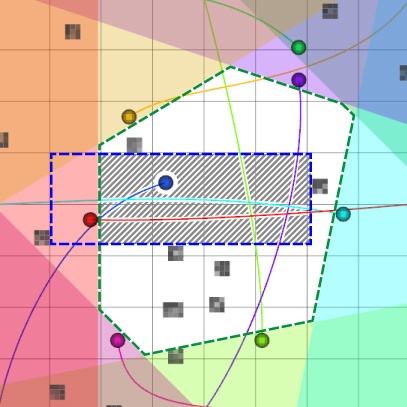
Figure 3: Collision avoidance constraints. The region surrounded by the blue dashed line is safe flight corridor (SFC) for the blue agent, and the region surrounded by green dashed line is the intersection of relative safe flight corridor (RSFC) for the blue agent. To generate a safe trajectory, there must exist intersection between SFC and RSFC (gray shaded area).

IV-A Initial Trajectory

An initial trajectory of the $i^{th}$ quadrotor, $\pi^{i}=\{\pi^{i}_{0},...,\pi^{i}_{M}\}$, is defined as a path that satisfies the following conditions for all $m=0,...,M$ and $i\neq j$:

$$\pi^{i}_{0}=s^{i},\pi^{i}_{M}=g^{i}$$ (11)

$$\langle\pi^{i}_{m-1},\pi^{i}_{m}\rangle\oplus\mathcal{C}^{i}_{obs}\subset\mathcal{F}$$ (12)

$$\langle\pi^{i,j}_{m-1},\pi^{i,j}_{m}\rangle\cap\mathcal{C}^{i,j}_{inter}=\emptyset$$ (13)

where $\langle\pi^{i}_{m-1},\pi^{i}_{m}\rangle=\{\alpha\pi^{i}_{m-1}+(1-\alpha)\pi^{i}_{m}\mid 0\leq\alpha\leq 1\}$ is a line segment between waypoints $\pi^{i}_{m-1}$ and $\pi^{i}_{m}$, and $\pi^{i,j}_{m}=\pi^{j}_{m}-\pi^{i}_{m}$. (12) shows that the initial trajectory does not collide with obstacles, and (13) means that the agents do not collide with other agents when all the agents move along their initial trajectory at constant velocity.

IV-B Safe Flight Corridor

The $m^{th}$ safe flight corridor (SFC) of the $i^{th}$ quadrotor, $\mathcal{S}^{i}_{m}$, is defined as a convex set satisfies following conditions:

$$\mathcal{S}^{i}_{m}\oplus\mathcal{C}^{i}_{obs}\subset\mathcal{F}$$ (14)

$$\langle\pi^{i}_{m-1},\pi^{i}_{m}\rangle\subset\mathcal{S}^{i}_{m}$$ (15)

The condition (14) shows that an agent in SFC does not collide with obstacles, so SFC can be used for obstacle collision avoidance.

IV-C Relative Safe Flight Corridor

The $m^{th}$ relative safe flight corridor (RSFC) between $i^{th}$ and the $j^{th}$ quadrotor, $\mathcal{R}^{i,j}_{m}$, is defined as a convex set that satisfies the following conditions:

$$\mathcal{R}^{i,j}_{m}\cap\mathcal{C}^{i,j}_{inter}=\emptyset$$ (16)

$$\langle\pi^{i,j}_{m-1},\pi^{i,j}_{m}\rangle\subset\mathcal{R}^{i,j}_{m}$$ (17)

If $\mathcal{R}^{i,j}_{m}$ includes $p^{i,j}(t)$ for $t\in[T_{m-1},T_{m}]$, then there is no collision between the $i^{th}$ and $j^{th}$ agents for $t\in[T_{m-1},T_{m}]$ due to (9) and (16). For this reason, we can use RSFC to avoid collision between agents.

V Method

In this section, we introduce the efficient trajectory planning algorithm using convex safe corridors. Alg. 1 shows the process of trajectory planning. We first plan initial trajectories (line 1), and we use them to determine safe flight corridor (SFC) (line 3) and relative safe flight corridor (RSFC) (line 5). After that, we compose quadratic programming (QP) problem using initial trajectories and safe corridors (line 8). Finally, we scale the total flight time to satisfy dynamic feasibility constraints (line 9). The detail of each process is described in the following subsections.

Input: start point $s^{i}$, goal point $g^{i}$ for agents $i\in\{1,...,N\}$, 3D occupancy map $\mathcal{E}$

Output: total flight time $T$, trajectory $p^{i}(t)$ for agents $i\in\{1,...,N\}$, $t\in[0,T]$

1 $\pi=(\pi^{1},...,\pi^{N})\leftarrow$ planInitialTraj($s^{\forall i}$, $g^{\forall i},\mathcal{E}$);

2 for $i\leftarrow 1$ to $N$ do

3       $\mathcal{S}^{i}=(\mathcal{S}^{i}_{0},...,\mathcal{S}^{i}_{M})\leftarrow$ buildSFC($\pi^{i},\mathcal{E}$);

4       for $j\leftarrow i+1$ to $N$ do

5             $\mathcal{R}^{i,j}=(\mathcal{R}^{i,j}_{0},...,\mathcal{R}^{i,j}_{M})\leftarrow$ buildRSFC($\pi^{i},\pi^{j}$);

6            

7       end for

8      

9 end for

10$p^{0}(t),...,p^{N}(t)\leftarrow$ trajOpt($\pi,\mathcal{S}^{\forall i},\mathcal{R}^{\forall i,j>i})$;

11 $T,p^{0}(t),...,p^{N}(t)\leftarrow$ timeScale($p^{0}(t),...,p^{N}(t)$);

return $T,p^{0}(t),...,p^{N}(t)$

Algorithm 1 Trajectory Planning Algorithm

V-A Initial Trajectory Planning

To plan an initial trajectory, we use a graph-based multi-agent pathfinding (MAPF) algorithm. Among various MAPF algorithms such as [16, 17], we choose enhanced conflict-based search (ECBS) for the following two reasons: (i) ECBS can find a suboptimal solution in a short time. Because the optimal MAPF algorithm is NP-complete [18], it could be better to use a suboptimal MAPF solver with respect to computation time. (ii) The ECBS algorithm is complete. To guarantee completeness of Alg. 1, individual submodules in the algorithm must be complete.

To utilize the graph-based ECBS in our problem, we formulate the planInitialTrajectory function in line 1, Alg 1 as follows. First, we translate the given 3D occupancy map into a 3D grid map with grid size $d$. Next, we set constraints which determine conflict in the ECBS algorithm to satisfy the condition (13). After that, we give start and goal points as the input and compute the initial trajectory. If start and goal points are not located on the 3D grid map, then we use the nearest grid points instead and append the start/goal points to both ends respectively.

V-B Safe Flight Corridor Construction

Alg. 2 shows the construction process of safe flight corridor (SFC). We initialize SFC to $\langle\pi^{i}_{m-1},\pi^{i}_{m}\rangle$ to fulfill the condition (15) (line 3). For all direction, we check whether SFC is expandable (line 5-9), and we expand SFC by a pre-specified length (line 10). This algorithm guarantees to return convex sets that satisfy the definition of SFC.

Input: initial trajectory $\pi^{i}$, 3D occupancy map $\mathcal{E}$

Output: safe flight corridor $\mathcal{S}^{i}=(\mathcal{S}^{i}_{0},...,\mathcal{S}^{i}_{M})$

1 $D\leftarrow\{\pm x,\pm y,\pm z\}$;

2 for $m\leftarrow 1$ to $M$ do

3       $\mathcal{S}^{i}_{m}\leftarrow\langle\pi^{i}_{m-1},\pi^{i}_{m}\rangle$;

4       while $D$ is not empty do

5             for $\mu$ in $D$ do

6                   if $\mathcal{S}^{i}_{m}$ cannot expand to direction $\mu$ then

7                         $D\leftarrow D\backslash\mu$

8                   end if

9                  

10             end for

11            expand $\mathcal{S}^{i}_{m}$ to all direction in $D$;

12            

13       end while

14      

15 end for

Algorithm 2 buildSFC

V-C Relative Safe Flight Corridor Construction

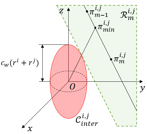
(a) Before coordinate transformation.

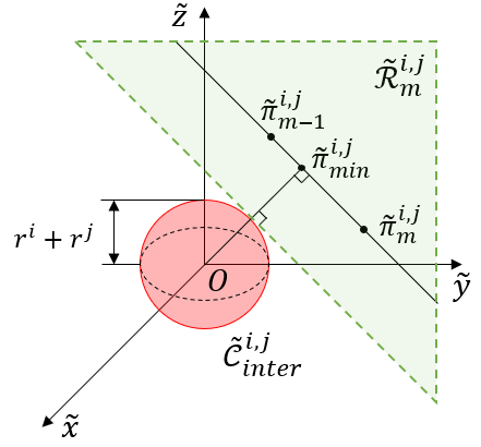
(b) After coordinate transformation.

Figure 4: Construction of relative safe flight corridor. The red ellipsoid is an inter-collision model between the quadrotors $i,j$, and the green-shaded region is the relative safe flight corridor (RSFC).

To build RSFC, we first perform affine coordinate transformation $\widetilde{x}=E^{\frac{1}{2}}x$, where $E^{\frac{1}{2}}$ is $diag([1,1,1/c_{dw}])$. Then, the inter-collision model $\mathcal{C}^{i,j}_{inter}$ and initial trajectory $\pi^{i,j}$ are transformed to $\widetilde{\mathcal{C}}^{i,j}_{inter}$ and $\widetilde{\pi}^{i,j}$ as shown in Fig. 4(b). Let $\widetilde{\pi}^{i,j}_{min}$ be the nearest point of $\langle\widetilde{\pi}^{i,j}_{m-1},\widetilde{\pi}^{i,j}_{m}\rangle$ to the origin. We construct RSFC as follows:

$$\mathcal{R}^{i,j}_{m}=\{x=E^{-\frac{1}{2}}\widetilde{x}\mid\widetilde{x}\cdot\widetilde{n}_{min}-(r^{i}+r^{j})>0\}$$ (18)

where $\widetilde{n}_{min}=\widetilde{\pi}^{i,j}_{min}/\|\widetilde{\pi}^{i,j}_{min}\|$. As depicted in Fig. 4(a), our RSFC is a half-space divided by the plane, which is tangent to the inter-collision model at the $\pi^{i,j}_{min}=E^{-\frac{1}{2}}\widetilde{\pi}^{i,j}_{min}$. We note that the convex set in (18) satisfies the definition of RSFC, but we omit the proof due to page limits.

V-D Sequential Trajectory Optimization

Optimizing all control points of polynomials at once can cause the scalability problem because the time complexity of the QP solver is $O(n^{3})$. Here, we propose an efficient sequential optimization method using dummy agents.

Input: initial trajectory $\pi$, safe flight corridor $\mathcal{S}^{\forall i}$, relative safe flight corridor $\mathcal{R}^{\forall i,j>i}$

Output: trajectory $p^{i}(t)$ for agents $i\in b$, $t\in[0,T]$

1 $p_{dmy}(t)=(p^{0}_{dmy}(t),...,p^{N}_{dmy}(t))\leftarrow$ planDummy($\pi$);

2 for $l\leftarrow 1$ to $N_{b}$ do

3       $b\leftarrow$ agents in $l^{th}$ batch;

4       $p^{b}(t)\leftarrow$ solveQP($\pi^{b},\mathcal{S}^{b},\mathcal{R}^{\forall i,j>i},p^{\forall i\notin b}_{dmy}(t)$);

5       $p_{dmy}(t)\leftarrow p(t)$;

6      

7 end for

return $p^{0}(t),...,p^{N}(t)$

Algorithm 3 trajOpt

Alg. 3 shows the process of sequential optimization. First, we generate trajectories for dummy agents $p_{dmy}(t)$ using the following control points (line 1):

$$c^{i}_{m,k}=\begin{cases}\ \pi^{i}_{m-1}&k=0,...,\phi-1\\ \ \pi^{i}_{m}&k=n-(\phi-1),...,n\\ \ x\in\langle\pi^{i}_{m-1},\pi^{i}_{m}\rangle&else\end{cases}$$ (19)

Next, we divide the agents into $N_{b}$ batches, and we solve the below QP problem for the batch $b$ (line 3-4):

minimize $$c^{T}Qc$$ (20)

subject to $$A_{eq}c=b_{eq}$$

$$c^{i}_{m,k}=\text{control points of }p^{i}_{dmy}(t), \forall i\notin b,m,k$$

$$c^{i}_{m,k}\in\mathcal{S}^{i}_{m}, \forall i\in b,m,k$$

$$c^{j}_{m,k}-c^{i}_{m,k}\in\mathcal{R}^{i,j}_{m} \forall i,j>i,m,k$$

where $c\in\mathbb{R}^{\frac{N}{N_{b}}M(n+1)}$, $A_{eq}\in\mathbb{R}^{\frac{N}{N_{b}}(M+1)\phi\times\frac{N}{N_{b}}M(n+1)}$, and the number of inequality constraints is $(N-\frac{1}{2}(\frac{N}{N_{b}}+1))\frac{N}{N_{b}}M(n+1)$. $p^{i}_{dmy}(t)$ is the trajectory for $i^{th}$ dummy agent. At last, we replace the trajectory of dummy agents to the previously planned one (line 5), and plan the trajectory for the next batch sequentially.

Fig. 5 visualizes the overall process. For each iteration, we deploy dummy agents except the agents in the current batch (Fig. 5(a)). Then, we plan the trajectory for the current batch to avoid dummy agents (Fig. 5(b)). After that, agents in the current batch are used as dummy agents at the next iteration (Fig. 5(c)). At the end of the iteration, collision-free trajectories are found without deadlock because all the agents are planned to avoid the previous batch (Fig. 5(d)).

This sequential method can achieve better scalability because we can avoid the high time complexity of QP solver by increasing the number of the batch as the number of agents increases while keeping the same number of decision variables of QP. Furthermore, we can prove that (20) consists of feasible constraints, which means that our method does not cause optimization failure due to infeasible constraints.

Theorem 1.

If $n\geq 2\phi-1$, then there exists a decision vector $c$ that satisfies the constraints of eq. (20) for all iterations.

Proof.

For any iteration $l$, let us assign the decision vector $c$ as (19) for $i\in b$ and $m=1,...,M$. Then $c$ satisfies the waypoint constraints due to (11). $p^{i}(t)$ is continuous up to $\phi-1^{th}$ derivatives at $t=T_{m}$ for $m=1,...,M-1$ because $c^{i}_{m,n-(\phi-1):n}=c^{i}_{m+1,0:\phi-1}=\pi^{i}_{m}$. $c$ also fulfills safe corridor constraints due to (15) and (17). Note that trajectories in the iteration $1,...,l-1$ do not collide with trajectories in the current batch because they are planned to avoid dummy agents which consist of control points (19). Thus, $c$ is the decision vector that satisfies the constraints of (20). ∎

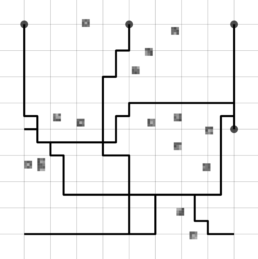
(a) Deploy dummy agents.

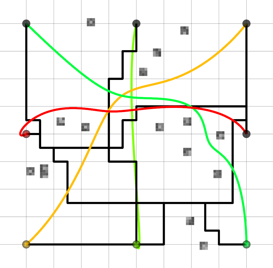
(b) Plan for one batch.

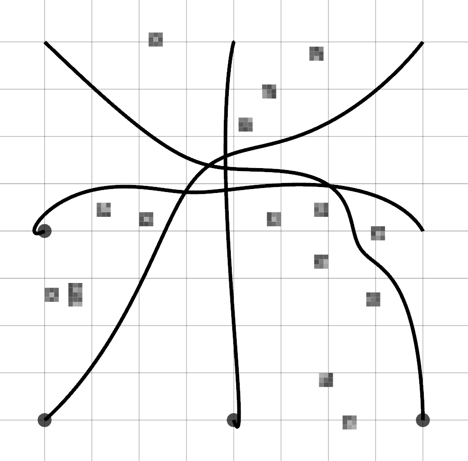
(c) Replace dummy agents with the previous batch.

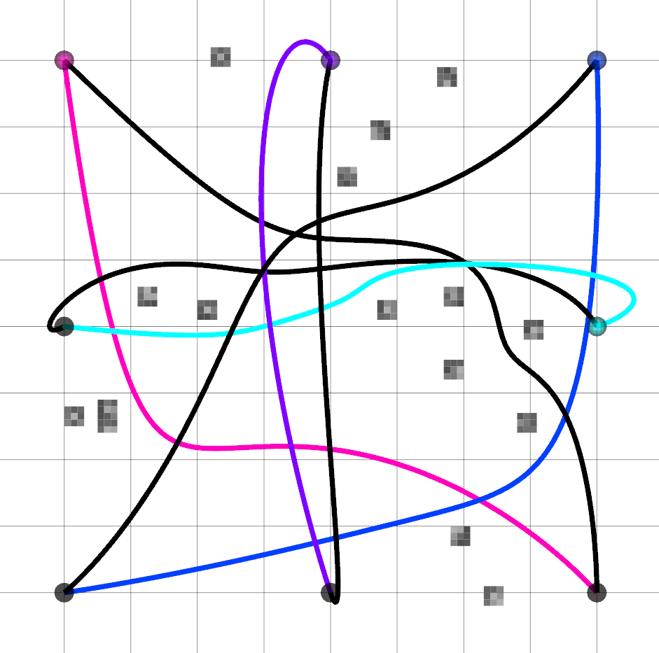
(d) Plan for next batch.

Figure 5: Sequential planning with dummy agents when $N_{b}=2$. Dummy agent is depicted as a black circle, and agent in the current batch is depicted as a colored circle. For each iteration, we plan a trajectory for the current batch (color line) that avoids the trajectory of dummy agents (black line).

In (20), we do not consider dynamic limits in the QP problem because they can be infeasible constraints for QP. Instead, similar to [9], we scale the total flight time for all agents uniformly after optimization (line 9 of Alg. 1).

VI EXPERIMENTS

VI-A Implementation Details

The proposed algorithm is run in C++ and executed the proposed algorithm on a PC running Ubuntu 18.04. with Intel Core i7-7700 @ 3.60GHz CPU and 16G RAM. We model the quadrotor with radius $r^{\forall i}=0.15$m, maximum velocity $v^{\forall i}_{max}=1.7m/s$, maximum acceleration $a^{\forall i}_{max}=6.2m/s^{2}$ and downwash coefficient $c_{dw}=2$ based on the specification of Crazyflie 2.0 in [10]. We use the Octomap library [19] to represent the 3D occupancy map and use CPLEX QP solver [20] for trajectory optimization. The degree of polynomials is determined to $n=5$ to satisfy the assumption in the Theorem 1. We plan the initial trajectory in 3D grid map with grid size $d=0.5$ m, and set suboptimal bound of ECBS to $1.3$.

VI-B Comparison with Previous Work

To validate the performance of our proposed algorithm, we compared the result with previous work [5]. We conducted the simulations in 50 random forests. Each forest has a size of 10 m $\times$ 10 m $\times$ 2.5 m and contains randomly deployed 20 trees of size 0.3 m $\times$ 0.3 m $\times$ 1–2.5 m. We assigned start point of quadrotors in a boundary of the xy-plane in 1 m height, and the goal points at the opposite to their start position as shown in Fig. 6.

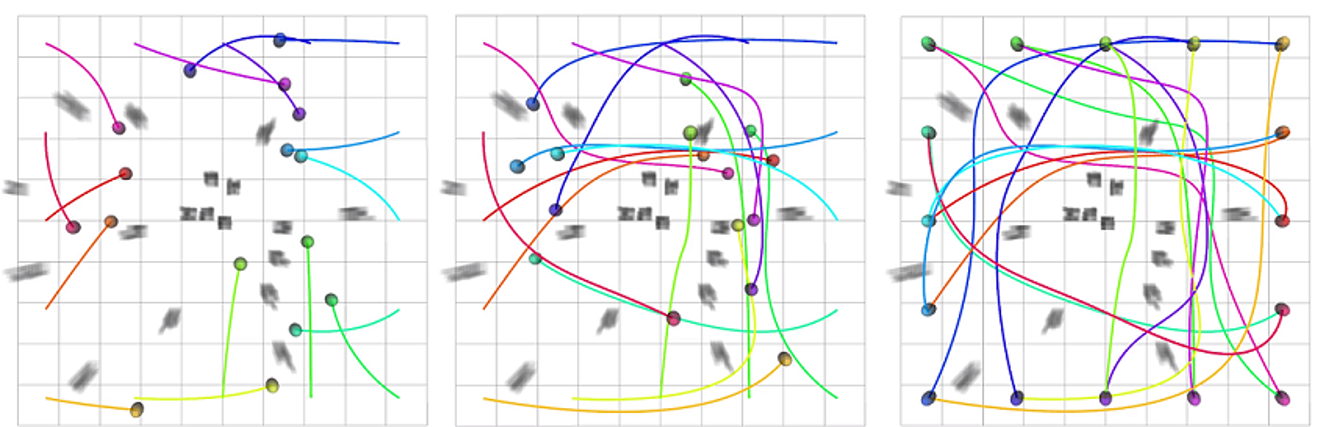
Figure 6: Trajectory generated for 16 agents in a 10 m $\times$ 10 m $\times$ 2.5 m random forest. Agents are marked with colored circles at the goal (assigned to the opposite of the start points), along with their trajectories.

VI-B1 Success Rate

We executed the simulation with 16 agents, and measured the success rate by the size of agents. As shown in the left graph of Fig. 7, both methods show a $100\%$ success rate in 50 random forest when the radius of agents is small, but the success rate of [5] decreases as the size of agents increases. It is because the larger the agent size, the smaller the space for agents can exist, which lead to the higher probability that the constraints for SFC and RSFC are infeasible each other. On the contrary, the proposed method shows a perfect success rate for all case because we design SFC and RSFC to feasible each other.

VI-B2 Solution Quality

As depicted in the right graph of Fig. 7, the proposed algorithm shows better performance with respect to both objective cost and computation time compare to previous work when the number of the batch $N_{b}$ is more than one. It can generate a trajectory for 64 agents in 6.36 s ($N_{b}=16$), and it has $78\%$ ($N_{b}=1$), $53\%$ ($N_{b}=16$) less objective cost. Note that we can adjust $N_{b}$ depending on the desired objective cost and computation time.

Table I: Computation time comparison with previous work [5]. The numbers in parentheses represent the computation time increment when the number of agents is doubled.

	Computation Time (s)
Agents	4	8	16	32	64
[5]	0.093	0.19 ($\times 2.0$)	0.81 ($\times 4.3$)	5.30 ($\times 6.5$)	51.1 ($\times 9.6$)
Proposed ($N_{b}=1$)	0.11	0.29 ($\times 2.7$)	1.15 ($\times 3.9$)	11.1 ($\times 9.6$)	197.0 ($\times 17.8$)
Proposed ($N/N_{b}=4$)	0.11	0.23 ($\times 2.2$)	0.59 ($\times 2.5$)	1.55 ($\times 2.6$)	6.36 ($\times 4.1$)

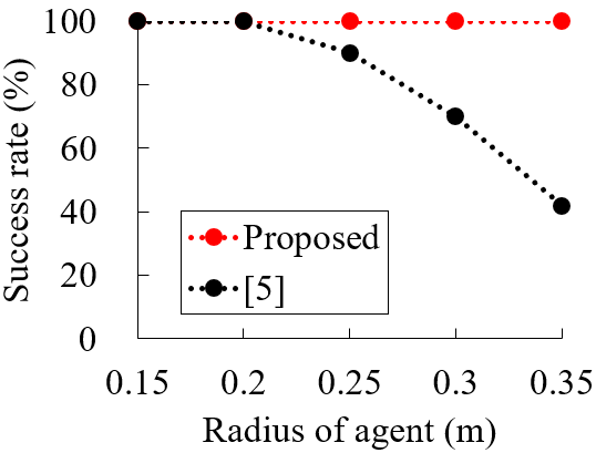
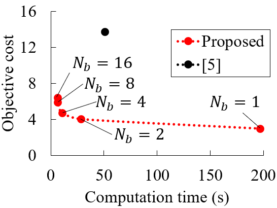
Figure 7: Comparison with previous work [5]. (Left) The success rate for 16 agents, (Right) Objective cost and computation time for 64 agents by the number of batches $N_{b}$.

VI-B3 Scalability Analysis

The computation time increment by the number of agents is shown in Table I. When the number of agents is small, the computation time increases linearly, regardless of the trajectory optimization method, but it follows the time complexity of QP solver as the number of agents increases if we do not adopt the sequential optimization method. On the other hand, if we maintain the size of the batch ($N/N_{b}$), it still shows good scalability with the high number of agents.

VI-C Comparison with SCP-based Method

We compared the proposed algorithm with SCP-based method [7]. Experiments are done in 10 m $\times$ 10 m $\times$ 2.5 m empty space with 8 agents. Start position and goal points are same as the previous experiment as shown in Fig. 8, and we assigned the same total flight time to both algorithm.

Table II shows that the proposed algorithm requires less computation time for all the cases, and this result does not change when we stop the SCP at the first iteration with collision avoidance constraints. The third column shows the safety margin ratio of each method. Safety margin ratio is calculated by $\text{min}_{i,j}d^{i,j}_{min}/(r^{i}+r^{j})$, where $d^{i,j}_{min}$ is a minimum distance between two agents $i,j$. Safety margin ratio must be over $100\%$ to guarantee the collision avoidance, however, SCP-based method does not satisfy this because SCP checks only collision avoidance between discrete points on each trajectory. On the contrary, the proposed method satisfies the safety condition completely.

Although the proposed method perform better in computation time and safety margin, it has longer total flight distance compared to the SCP method. It is because our initial trajectory is not optimal respect to total flight distance in non-grid space. Thus, we need to plan initial trajectory considering total flight distance, and leave it as future work.

Table II: Comparison of proposed algorithm and SCP-based method.

	Comp. Time per Iter. (s)	Total Comp. Time (s)	Safety Margin Ratio	Total Flight Dist. (m)
SCP ($h=1.0$ s)	0.78	2.80	$12\%$	77.29
SCP ($h=0.5$ s)	5.5	20.5	$81\%$	77.36
SCP ($h=0.34$ s)	16.2	60.4	$92\%$	77.38
SCP ($h=0.25$ s)	42.1	156.6	$96\%$	77.40
Proposed ($N_{b}=1$)	-	0.65	101$\%$	90.74

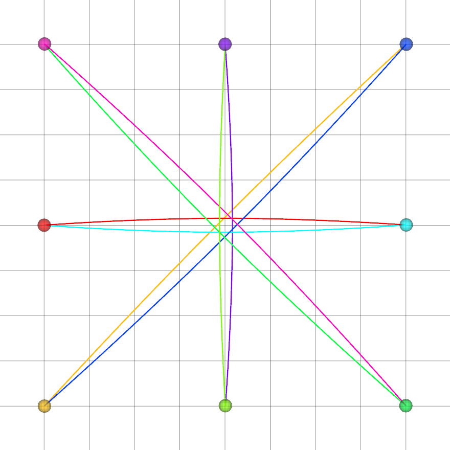
(a) SCP-based [7]

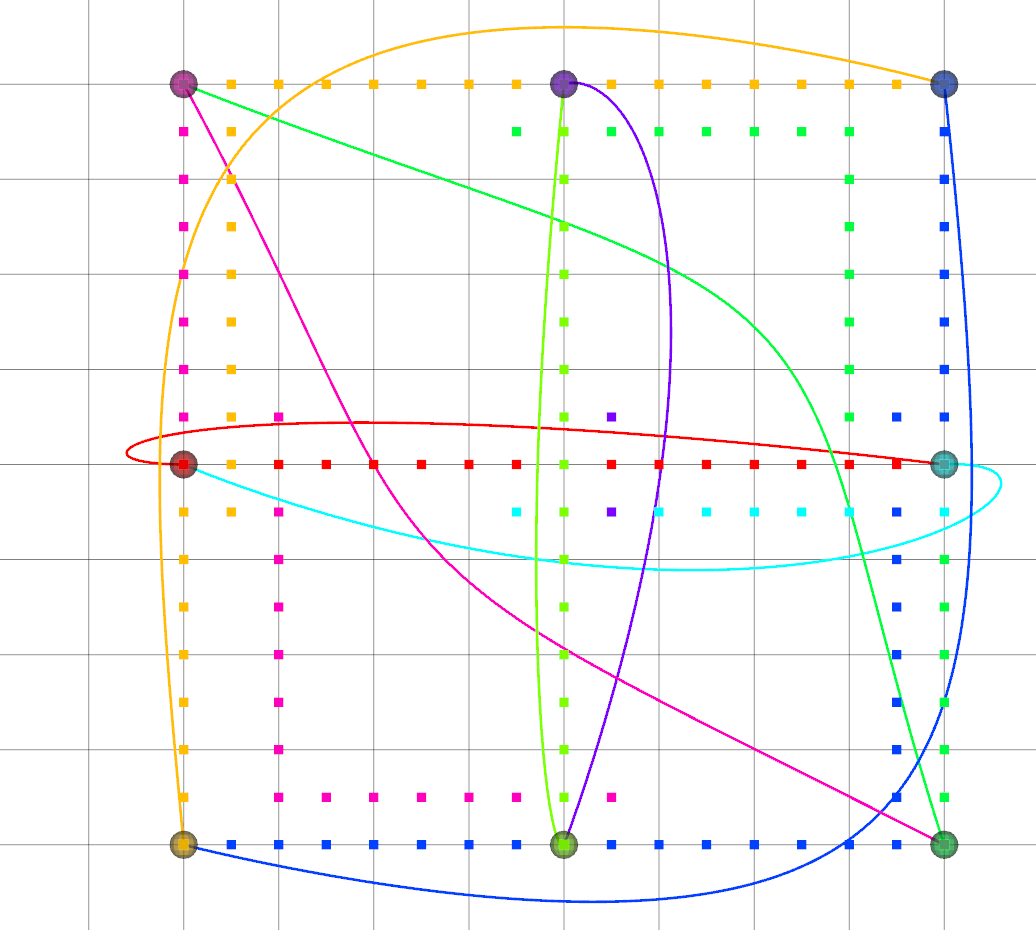
(b) Proposed

Figure 8: Trajectory planning result of the propose algorithm and SCP-based method in empty space. The dots in (b) are the initial trajectory of corresponding agents.

VI-D Flight Test

We conducted real flight test with 6 Crazyflie 2.0 quadrotors in a 5 m x 7 m x 2.5 m space. We used Crazyswarm [21] to follow the pre-computed trajectory, and we used Vicon motion capture system to obtain the position information at 100 Hz. The snapshot of the flight test is shown in Fig. 1, and the full flight is presented in the supplemental video.

VII CONCLUSIONS

We presented an efficient trajectory planning algorithm for multiple quadrotors in obstacle environments, combining the advantages of grid-based and optimization-based planning algorithm. Using relative Bernstein polynomial, we reformulated trajectory generation problem to convex optimization problem, which guarantees to generate continuous, collision-free, and dynamically feasible trajectory. We improved the scalability of the algorithm by using sequential optimization method, and we proved overall process does not cause the failure of optimization if there exist initial trajectory. The proposed algorithm shows considerable reduction in computation time and objective cost compared to our previous work, and it shows better performance in computation time and safety, compared to SCP-based method.

In future work, we plan to develop initial trajectory planner that optimizes total flight distance in non-grid space, and we will extend our work to dynamic obstacle environment.

References

- [1] Daman Bareiss and Jur Berg “Reciprocal collision avoidance for robots with linear dynamics using lqr-obstacles” In Robotics and Automation (ICRA), 2013 IEEE International Conference on, 2013, pp. 3847–3853 IEEE
- [2] Dingjiang Zhou, Zijian Wang, Saptarshi Bandyopadhyay and Mac Schwager “Fast, on-line collision avoidance for dynamic vehicles using buffered voronoi cells” In IEEE Robotics and Automation Letters 2.2 IEEE, 2017, pp. 1047–1054
- [3] Yufan Chen, Mark Cutler and Jonathan P How “Decoupled multiagent path planning via incremental sequential convex programming” In Robotics and Automation (ICRA), 2015 IEEE International Conference on, 2015, pp. 5954–5961 IEEE
- [4] Carlos E Luis and Angela P Schoellig “Trajectory generation for multiagent point-to-point transitions via distributed model predictive control” In IEEE Robotics and Automation Letters 4.2 IEEE, 2019, pp. 375–382
- [5] Jungwon Park and H. Jin Kim “Fast Trajectory Planning for Multiple Quadrotors using Relative Safe Flight Corridor”, 2019 eprint: arXiv:1909.02896
- [6] Daniel Mellinger, Alex Kushleyev and Vijay Kumar “Mixed-integer quadratic program trajectory generation for heterogeneous quadrotor teams” In Robotics and Automation (ICRA), 2012 IEEE International Conference on, 2012, pp. 477–483 IEEE
- [7] Federico Augugliaro, Angela P Schoellig and Raffaello D’Andrea “Generation of collision-free trajectories for a quadrocopter fleet: A sequential convex programming approach” In Intelligent Robots and Systems (IROS), 2012 IEEE/RSJ International Conference on, 2012, pp. 1917–1922 IEEE
- [8] D Reed Robinson, Robert T Mar, Katia Estabridis and Gary Hewer “An Efficient Algorithm for Optimal Trajectory Generation for Heterogeneous Multi-Agent Systems in Non-Convex Environments” In IEEE Robotics and Automation Letters 3.2 IEEE, 2018, pp. 1215–1222
- [9] Wolfgang Hönig et al. “Trajectory planning for quadrotor swarms” In IEEE Transactions on Robotics 34.4 IEEE, 2018, pp. 856–869
- [10] Mark Debord, Wolfgang Hönig and Nora Ayanian “Trajectory planning for heterogeneous robot teams” In 2018 IEEE/RSJ International Conference on Intelligent Robots and Systems (IROS), 2018, pp. 7924–7931 IEEE
- [11] Daniel Mellinger and Vijay Kumar “Minimum snap trajectory generation and control for quadrotors” In Robotics and Automation (ICRA), 2011 IEEE International Conference on, 2011, pp. 2520–2525 IEEE
- [12] Mark W Mueller, Markus Hehn and Raffaello D’Andrea “A computationally efficient motion primitive for quadrocopter trajectory generation” In IEEE Transactions on Robotics 31.6 IEEE, 2015, pp. 1294–1310
- [13] Michael Zettler and Jürgen Garloff “Robustness analysis of polynomials with polynomial parameter dependency using Bernstein expansion” In IEEE Transactions on Automatic Control 43.3 IEEE, 1998, pp. 425–431
- [14] Sarah Tang and Vijay Kumar “Safe and complete trajectory generation for robot teams with higher-order dynamics” In 2016 IEEE/RSJ International Conference on Intelligent Robots and Systems (IROS), 2016, pp. 1894–1901 IEEE
- [15] Fei Gao, William Wu, Yi Lin and Shaojie Shen “Online safe trajectory generation for quadrotors using fast marching method and bernstein basis polynomial” In 2018 IEEE International Conference on Robotics and Automation (ICRA), 2018, pp. 344–351 IEEE
- [16] Glenn Wagner and Howie Choset “M*: A complete multirobot path planning algorithm with performance bounds” In 2011 IEEE/RSJ International Conference on Intelligent Robots and Systems, 2011, pp. 3260–3267 IEEE
- [17] Guni Sharon, Roni Stern, Ariel Felner and Nathan R Sturtevant “Conflict-based search for optimal multi-agent pathfinding” In Artificial Intelligence 219 Elsevier, 2015, pp. 40–66
- [18] Jingjin Yu and Steven M LaValle “Structure and intractability of optimal multi-robot path planning on graphs” In Twenty-Seventh AAAI Conference on Artificial Intelligence, 2013
- [19] Armin Hornung et al. “OctoMap: An efficient probabilistic 3D mapping framework based on octrees” In Autonomous robots 34.3 Springer, 2013, pp. 189–206
- [20] ILOG CPLEX “12.7. 0 User’s Manual” IBM, 2016
- [21] James A Preiss, Wolfgang Honig, Gaurav S Sukhatme and Nora Ayanian “Crazyswarm: A large nano-quadcopter swarm” In Robotics and Automation (ICRA), 2017 IEEE International Conference on, 2017, pp. 3299–3304 IEEE