A second-order and nonuniform time-stepping maximum-principle preserving scheme for time-fractional Allen-Cahn equations

Abstract

In this work, we present a second-order nonuniform time-stepping scheme for the time-fractional Allen-Cahn equation. We show that the proposed scheme preserves the discrete maximum principle, and by using the convolution structure of consistency error, we present sharp maximum-norm error estimates which reflect the temporal regularity. As our analysis is built on nonuniform time steps, we may resolve the intrinsic initial singularity by using the graded meshes. Moreover, we propose an adaptive time-stepping strategy for large time simulations. Numerical experiments are presented to show the effectiveness of the proposed scheme. This seems to be the first second-order maximum principle preserving scheme for the time-fractional Allen-Cahn equation.

Keywords:   Time-fractional Allen-Cahn equation; Alikhanov formula; adaptive time-stepping strategy; discrete maximum principle; sharp error estimate

AMS subject classiffications.   35Q99, 65M06, 65M12, 74A50

1 Introduction

We consider the following two dimensional time-fractional Allen-Cahn equation

$$\partial_{t}^{\alpha}u(\mathbf{x},0)= \,\varepsilon^{2}\Delta{u}-f(u),\quad\mathbf{x}\in\Omega,\quad{0}<{t}\leq{T},$$ (1.1)

$$u(\mathbf{x},0)= \,u_{0}(\mathbf{x}),\quad\mathbf{x}\in\bar{\Omega},$$ (1.2)

where $\Omega=(0,L)^{2}$ with closure $\bar{\Omega}$. The nonlinear bulk force $f(u)$ is given by $f(u)=u^{3}-u.$ The constant $0<\varepsilon\ll 1$ is the interaction length that describes the thickness of the transition boundary between materials. For simplicity, we consider the periodic boundary conditions. In equations (1.1), $\partial_{t}^{\alpha}:={}_{0}^{C}\!D_{t}^{\alpha}$ denotes the Caputo derivative of order $\alpha:$

$$(\partial_{t}^{\alpha}v)(t):=(\mathcal{I}_{t}^{1-\alpha}v^{\prime})(t)=\int_{0}^{t}\omega_{1-\alpha}(t-s)v^{\prime}(s)\,\mathrm{d}{s},\quad 0<\alpha<1,$$ (1.3)

where $\mathcal{I}_{t}^{\mu}$ is the fractional Riemann-Liouville integral of order $\mu>0$, that is,

$$(\mathcal{I}_{t}^{\mu}v)(t):=\int_{0}^{t}\omega_{\mu}(t-s)v(s)\,\mathrm{d}{s},\quad\text{where}\quad\omega_{\mu}(t):=t^{\mu-1}/\Gamma(\mu).$$ (1.4)

As a generalization of the classical Allen-Cahn equation [2, 8, 25, 6], the above time-fractional Allen-Cahn equation (1.1) has been widely investigated in recent years [11, 15, 22, 28], In particular, it was first shown in [28] that the time-fractional Allen-Cahn equation admits the following energy law

$$E(t)\leq{E}(0),$$ (1.5)

where $E(t)$ is the total energy defined by

$$E(t):=\int_{\Omega}\left[\frac{\varepsilon^{2}}{2}|\nabla{u}|^{2}+F(u)\right]\,\mathrm{d}{\mathbf{x}},\quad F(u)=\frac{1}{4}(1-u^{2})^{2}.$$ (1.6)

Moreover, the following maximum principle holds [28]

$$|u(\mathbf{x},t)|\leq{1}\quad\text{if}\quad|u(\mathbf{x},0)|\leq{1}.$$ (1.7)

From the numerical scheme point of view, first order schemes that combine the $L1$ formula [21, 27] and the stabilization technique [29] were proposed in [28] for the time-fractional Allen-Cahn equation. Furthermore, it is shown in [28] that the stabilization $L1$ scheme preserves the energy law (1.5) and the maximum principle (1.7) in the discrete level. More recently, sharp regularity analysis of the time-fractional Allen-Cahn equation and numerical analysis for a class of numerical schemes under limited regularity were presented in [5]. Notice that all the analysis in the above mentioned works is based on uniform time grids.

In this work, we aim at designing a second order scheme using nonuniform time grids. There are two main motivations to investigate nonuniform time grids:

• Similar as in other nonlinear subdiffusion problems, the solution of the time-fractional Allen-Cahn equation admits an intrinsic initial singularity [13]. Consequently, graded meshes are recommended for such problems [26, 3].

• The solution of the time-fractional Allen-Cahn equation may admit multiple time scales [7, 24, 14, 4, 9], i.e., the initial dynamics evolve on a fast time scale and later coarsening stage evolves on a very slow time scale. Therefore, one may need to use adaptive time grids to catch different time scales [24, 30].

To this end, we present in this work a second order Alikhanov-type scheme under nonuniform time grids. We shown that the proposed scheme preserves the discrete maximum principle, and this seems to be the first work on second order maximum principle preserving schemes for the time-fractional Allen-Cahn equation. We also present a sharp maximum-norm error estimate the can reflect the temporal regularity. Finally, we propose an adaptive time-stepping strategy for long-time simulations.

The rest of this work is organized as follows. We present some preliminaries in Section 2. A second order nonuniform Alikhanov scheme is proposed in Section 3, where the discrete maximum principle is also established. The convergence analysis of the proposed scheme is given in section 4, and this is followed by extensive experiments in Section 5. We finally give some concluding remarks in Section 6.

2 Preliminaries

In this section, we shall present some preliminaries.

2.1 Nonuniform time grids

Throughout the paper, we shall consider nonuniform time grids. To this end, we introduce the following time mesh:

$${}0=t_{0}<t_{1}<\cdots<t_{k-1}<t_{k}<\cdots<t_{N}=T$$ (2.1)

with time-step sizes $\tau_{k}:=t_{k}-t_{k-1}$ for $1\leq{k}\leq{N}.$ We define the maximum time-step size as $\tau:=\max_{1\leq{k}\leq{N}}\tau_{k}$. Also, for $k\geq{1}$ and $0<\theta<1$ we define the off-set time level as $t_{k-\theta}:=(1-\theta)t_{k}+\theta t_{k-1}.$ We set the adjacent step ratio as $\rho_{k}:=\tau_{k}/\tau_{k+1}$ and define the maximum step ratio as $\rho:=\max_{k\geq 1}\rho_{k}$. We now introduce the following assumptions.

1. The maximum time-step ratio $\rho=7/4$.

The condition M1 says that one can use a series of decreasing time-steps with the reduction factor down to $4/7$. Always, we do not impose any restrictions to the amplification factor for increasing time-steps, although a maximum time-step size may be necessary for theocratical analysis. The use of nonuniform meshes are motivated by the following two reasons: Firstly, to resolve the initial solution singularity $u_{t}\sim\mathcal{O}(t^{\alpha-1})$ as $t\rightarrow 0$, a graded mesh $t_{k}=T(k/N)^{\gamma}$ with the step ratios $\rho_{k}\leq 1$ has been a popular approach in recent years [26]. Secondly, to capture the fast dynamics away from $t=0$ and the slowly coarsening stage near the steady state, one may use an adaptive time-stepping strategy [24, 14]. We also need the following assumption for the sake of convergence analysis [16, 19, 23]:

1. For a parameter $\gamma\geq{1}$, there exists mesh-independent constants $C_{1\gamma},C_{2\gamma}>0$ such that $\tau_{k}\leq\tau\min\{1,C_{1\gamma}t_{k}^{1-1/\gamma}\}$ for $1\leq k\leq N$ and $t_{k}\leq C_{2\gamma}t_{k-1}$ for $2\leq{k}\leq{N}$.

Here, the parameter $\gamma\geq 1$ controls the extent to which the time levels are concentrated near $t=0$. If the mesh is quasi-uniform, then M2 holds with $\gamma=1$. As $\gamma$ increases, the initial step sizes become smaller compared to the later ones.

To facilitate the error analysis of difference approximations in space, we assume that the continuous solution $u$ is sufficiently smooth in physical domain and satisfies

$$\big{\|}u(t)\big{\|}_{W^{4,\infty}(\Omega)}\leq{C}_{u},\quad\big{\|}u^{(\ell)}(t)\big{\|}_{W^{2,\infty}(\Omega)}\leq{C}_{u}\big{(}1+t^{\sigma-\ell}\big{)}\;\;\text{for $\ell=1,2,3$,}$$ (2.2)

where a regularity parameter $\sigma\in(0,1)$ is introduced to make our analysis extendable. In what follows, we use subscripted $C$, such as $C_{\gamma}$, $C_{v}$ and $C_{u}$, to denote a generic positive constant, which is not necessarily the same at different occurrences, yet is always dependent on the given data and the solution but independent of temporal and spatial mesh sizes.

2.2 Discrete fractional Grönwall lemma

We recall the recent developed discrete fractional Grönwall inequality that involves the well-known Mittag–Leffler function $E_{\alpha}(z):=\sum_{k=0}^{\infty}\frac{z^{k}}{\Gamma(1+k\alpha)}$ in [18, Lemma 2.2, Theorems 3.1-3.2].

Lemma 2.1

For $n=1,2,\cdots,N$, assume that the discrete convolution kernels $\{A_{n-k}^{(n)}\}_{k=1}^{n}$ satisfy the following two assumptions:
Ass1. There is a constant $\pi_{A}>0$ such that $A_{n-k}^{(n)}\geq\frac{1}{\pi_{A}\tau_{k}}\int_{t_{k-1}}^{t_{k}}\omega_{1-\alpha}(t_{n}-s)\,\mathrm{d}s$ for $1\leq k\leq n$.
Ass2. The discrete kernels are monotone, i.e. $A_{n-k-1}^{(n)}\geq A_{n-k}^{(n)}$ for $1\leq k\leq n-1$.
We define a sequence of discrete complementary convolution kernels $\{P_{n-j}^{(n)}\}_{j=1}^{n}$ by

$$P_{0}^{(n)}:=\frac{1}{A_{0}^{(n)}},\quad P_{n-j}^{(n)}:=\frac{1}{p_{0}^{(j)}}\sum_{k=j+1}^{n}\big{(}A_{k-j-1}^{(k)}-A_{k-j}^{(k)}\big{)}P_{n-k}^{(n)},\quad 1\leq j\leq n-1.$$ (2.3)

Then the discrete complementary convolution kernels $P^{(n)}_{n-j}\geq 0$ fulfill

$$\sum_{j=k}^{n}P^{(n)}_{n-j}A_{j-k}^{(j)}\equiv 1,\quad\text{for $1\leq k\leq n\leq N$.}$$ (2.4)

$$\sum_{j=1}^{n}P^{(n)}_{n-j}\omega_{1+m\alpha-\alpha}(t_{j})\leq\pi_{A}\omega_{1+m\alpha}(t_{n}),\quad\text{for $m=0,1$ and $1\leq n\leq N$.}$$ (2.5)

Suppose that $\lambda_{0}$ and $\lambda_{1}$ are non-negative constants independent of the time-steps, $\lambda:=\lambda_{0}+\lambda_{1}$ and the maximum step size $\tau\leq 1/\sqrt[\alpha]{2\Gamma(2-\alpha)\lambda\pi_{A}}.$ If the non-negative sequences $(v^{k})_{k=0}^{N}$, $(\xi^{k})_{k=1}^{N}$ and $(\eta^{k})_{k=1}^{N}$ satisfy

$$\sum_{k=1}^{n}A_{n-k}^{(n)}\triangledown_{\tau}v^{k}\leq\lambda_{0}v^{n}+\lambda_{1}v^{n-1}+\xi^{n}+\eta^{n}\quad\text{for\ $1\leq n\leq N$,}$$ (2.6)

then for $1\leq n\leq N$ it holds that

$$v^{n} \leq 2E_{\alpha}\big{(}2\max\{1,\rho\}\lambda\pi_{A}t_{n}^{\alpha}\big{)}\Big{(}v^{0}+\max_{1\leq k\leq n}\sum_{j=1}^{k}P^{(k)}_{k-j}(\xi^{j}+\eta^{j})\Big{)}$$

$$\leq 2E_{\alpha}\big{(}2\max\{1,\rho\}\lambda\pi_{A}t_{n}^{\alpha}\big{)}\Big{(}v^{0}+\Gamma(1-\alpha)\pi_{A}\max_{1\leq k\leq n}\{t_{k}^{\alpha}\xi^{k}\}+\pi_{A}\omega_{1+\alpha}(t_{n})\max_{1\leq k\leq n}\eta^{k}\Big{)}.$$

3 A second-order maximum principle preserving scheme

In this section, we shall present our second order fully discrete scheme for the time-fractional Allen-Cahn equation (1.1)-(1.2). In what follows, we consider $\theta:=\alpha/2.$

3.1 The Alikhanov formula under nonuniform grids

Given a grid function $\{v^{k}\}$ that is defined on a nonuniform grid (2.1), for $k\geq{1},$ we define the difference operator $\triangledown_{\tau}v^{k}:=v^{k}-v^{k-1}$, the difference quotient operator $\partial_{\tau}v^{k-\frac{1}{2}}:=\triangledown_{\tau}v^{k}/\tau_{k}$ and the weighted operator $v^{k-\theta}:=(1-\theta)v^{k}+\theta v^{k-1}$. We then denote by $\Pi_{1,k}v$ the linear interpolant of a function $v$ with respect to the nodes $t_{k-1}$ and $t_{k}$, and by $\Pi_{2,k}v$ the quadratic with respect to the nodes $t_{k-1},t_{k}$ and $t_{k+1}$. The corresponding interpolation errors are denoted by $\big{(}\widetilde{\Pi_{\nu,k}}v\big{)}(t):=v(t)-\left(\Pi_{\nu,k}v\right)(t)$ for $\nu=1,2$.

Recalling that $\rho_{k}=\tau_{k}/\tau_{k+1}$, then it is easy to show (by using the Newton form of the interpolating polynomials) that

$$\big{(}\Pi_{1,k}v\big{)}^{\prime}(t)=\frac{\triangledown_{\tau}v^{k}}{\tau_{k}}\quad\text{and}\quad\big{(}\Pi_{2,k}v\big{)}^{\prime}(t)=\frac{\triangledown_{\tau}v^{k}}{\tau_{k}}+\frac{2(t-t_{k-1/2})}{\tau_{k}(\tau_{k}+\tau_{k+1})}\Big{(}\rho_{k}\triangledown_{\tau}v^{k+1}-\triangledown_{\tau}v^{k}\Big{)}.$$

The nonuniform Alikhanov approximation [20, 17] to $(\partial_{t}^{\alpha}v)(t_{n-\theta})$ is defined by

$$(\partial_{\tau}^{\alpha}v)^{n-\theta}:= \,\int_{t_{n-1}}^{t_{n-\theta}}\omega_{1-\alpha}(t_{n-\theta}-s)\left(\Pi_{1,n}v\right)^{\prime}(s)\,\mathrm{d}{s}+\sum_{k=1}^{n-1}\int_{t_{k-1}}^{t_{k}}\omega_{1-\alpha}(t_{n-\theta}-s)\left(\Pi_{2,k}v\right)^{\prime}(s)\,\mathrm{d}{s}$$

$$= \,a^{(n)}_{0}\triangledown_{\tau}v^{n}+\sum_{k=1}^{n-1}\Big{(}a^{(n)}_{n-k}\triangledown_{\tau}v^{k}+\rho_{k}b^{(n)}_{n-k}\triangledown_{\tau}v^{k+1}-b^{(n)}_{n-k}\triangledown_{\tau}v^{k}\Big{)}.$$ (3.1)

Here and hereafter, we set $\sum_{k=i}^{j}\cdot=0$ if $i>j$. The associated discrete convolution kernels $a_{n-k}^{(n)}$ and $b_{n-k}^{(n)}$ are defined, respectively, as

$$a_{n-k}^{(n)} :=\frac{1}{\tau_{k}}\int_{t_{k-1}}^{\min\{t_{k},t_{n-\theta}\}}\omega_{1-\alpha}(t_{n-\theta}-s)\,\mathrm{d}{s},\quad 1\leq{k}\leq{n};$$ (3.2)

$$b_{n-k}^{(n)} :=\frac{2}{\tau_{k}(\tau_{k}+\tau_{k+1})}\int_{t_{k-1}}^{t_{k}}(s-t_{k-\frac{1}{2}})\omega_{1-\alpha}(t_{n-\theta}-s)\,\mathrm{d}{s},\quad 1\leq{k}\leq{n-1}.$$ (3.3)

By re-organizing the terms in (3.1) we obtain the following compact form

$$\left(\partial_{\tau}^{\alpha}v\right)^{n-\theta}:=\sum_{k=1}^{n}A_{n-k}^{(n)}\triangledown_{\tau}v^{k},$$ (3.4)

where the discrete kernels $A_{n-k}^{(n)}$ are defined by: $A_{0}^{(1)}:=a_{0}^{(1)}$ if $n=1$ and for $n\geq{2}$,

$$A_{n-k}^{(n)}:=\begin{cases}a_{0}^{(n)}+\rho_{n-1}b_{1}^{(n)},&\text{for}\;k=n,\vspace{2mm}\\ a_{n-k}^{(n)}+\rho_{k-1}b_{n-k+1}^{(n)}-b_{n-k}^{(n)},&\text{for}\;2\leq{k}\leq{n-1},\vspace{2mm}\\ a_{n-1}^{(n)}-b_{n-1}^{(n)},&\text{for}\;k=1.\end{cases}$$ (3.5)

Notice that the above nonuniform formula is an extension of the Alikhanov Formula on the uniform mesh [1], where the positiveness and monotonicity of $A_{n-k}^{(n)}=A_{n-k}$ were established. The nonuniform version (3.4) was first proposed in [20] to resolve the initial singularity by using a graded mesh near the initial time. Recently, the following results are presented in [17, Theorem 2.2]:

Lemma 3.1

Let M1 hold and consider the discrete convolution kernels $A_{n-k}^{(n)}$ in (3.5).

• The discrete kernels $A_{n-k}^{(n)}$ fulfill $A^{(n)}_{0}\leq\frac{24}{11\tau_{n}}\int_{t_{n-1}}^{t_{n}}\omega_{1-\alpha}(t_{n}-s)\,\mathrm{d}{s}$ and

  $$A^{(n)}_{n-k}\geq\frac{4}{11\tau_{n}}\int_{t_{n-1}}^{t_{n}}\omega_{1-\alpha}(t_{n}-s)\,\mathrm{d}{s},\quad 1\leq{k}\leq{n};$$

• The discrete kernels $A_{n-k}^{(n)}$ are monotone for $1\leq{k}\leq{n-1}$,

  $$A^{(n)}_{n-k-1}-A^{(n)}_{n-k}\geq(1+\rho_{k})b^{(n)}_{n-k}-\frac{1}{5\tau_{k}}\int_{t_{k-1}}^{t_{k}}(t_{k}-s)\omega_{-\alpha}(t_{n-\theta}-s)\,\mathrm{d}{s}>0.$$

• And the first kernel $A^{(n)}_{0}$ is appropriately larger than the second one,

  $$\frac{1-2\theta}{1-\theta}A^{(n)}_{0}-A^{(n)}_{1}>0\quad for\quad n\geq{2}.$$

We remark that the estimates in Lemma 3.1 are much more stronger than the previous results in [1, 20] on the uniform mesh, and these estimates will play an important role when analyzing our adaptive time stepping schemes for phase field equations (e.g., the Allen-Cahn equation in this work). In particular, the boundedness and monotonicity of $A_{n-k}^{(n)}$ are essential to verify the discrete maximum principle of our second-order time-stepping scheme for the Allen-Cahn equation.

Lemma 3.1 also implies that the discrete convolution kernels $A_{n-k}^{(n)}$ satisfy the two assumptions Ass1-Ass2 in Lemma 2.1 with $\pi_{A}=\frac{11}{4}$, and this will be adapted to show the convergence analysis of our time-stepping scheme using the discrete complementary convolution kernel argument.

3.2 The second order fully discrete scheme

To present the fully discrete scheme, we recall briefly the difference approximation in physical domain. For a positive integer $M$, let the spatial length $h:=L/M$. Also, we denote $\bar{\Omega}_{h}:=\big{\{}\mathbf{x}_{h}=(ih,jh)\,|\,0\leq i,j\leq M\}$ and set $\Omega_{h}:=\bar{\Omega}_{h}\cap\Omega$. For any grid function $\{v_{h}\,|\,\mathbf{x}_{h}\in\bar{\Omega}_{h}\}$, we denote the grid function space as

$$\mathbb{V}_{h}:=\big{\{}v\,|\,v=(v_{j})^{T}\;\;\text{for}\;\;1\leq{j}\leq{M},\;\;\text{with}\;\;v_{j}=(v_{i,j})^{T}\;\;\text{for}\;\;1\leq{i}\leq{M}\big{\}},$$

where $v^{T}$ is the transpose of the vector $v$. The maximum norm $\|v\|_{\infty}$ is defined as $\|v\|_{\infty}:=\max_{\mathbf{x}_{h}\in\Omega_{h}}|v_{h}|$.

We shall use the center difference scheme for discetizing the Laplace operator $\Delta$ subject to periodic boundary conditions. To this end, we denote by $D_{h}$ the associated discrete matrix, then we have $D_{h}=I\otimes{D}+D\otimes{I}$ with $\otimes$ being the Kronecker tensor product operator and

$$D=\frac{1}{h^{2}}\left(\begin{array}[]{ccccc}-2&1&0&\cdots&1\\ 1&-2&1&\cdots&0\\ \vdots&\ddots&\ddots&\ddots&\vdots\\ 0&\cdots&1&-2&1\\ 1&\cdots&0&1&-2\\ \end{array}\right)_{M\times{M}}.$$

We are now ready to present our time-weighted difference scheme for (1.1)-(1.2):

$$\big{(}\partial_{\tau}^{\alpha}u\big{)}^{n-\theta} =\varepsilon^{2}D_{h}u^{n-\theta}-f(u)^{n-\theta},\quad{n}\geq{1},$$ (3.6)

$$u_{h}^{0} =u_{0}(\mathbf{x}_{h}),\quad\mathbf{x}_{h}\in\bar{\Omega}_{h},$$ (3.7)

where the weighted nonlinear term $f(u)^{n-\theta}$ is given by

$$f(u)^{n-\theta}:=\theta{f}(u^{n-1})+(1-\theta)f(u^{n}),$$

and the vector $f(u^{n})$ is defined in the element-wise: $f(u^{n}):=(u^{n})^{.3}-u^{n}$.

To show the uniquely solvability of the above scheme, we list some useful properties of the matrix $D_{h}:$

Lemma 3.2

The discrete matrix $D_{h}$ has the following properties

• The discrete matrix $D_{h}$ is symmetric.

• For any nonzero $v\in{\mathbb{V}_{h}}$, $v^{T}D_{h}v\leq{0}$, i.e., the matrix $D_{h}$ is negative semi-definite.

• The elements of $D_{h}=(d_{ij})$ fulfill $d_{ii}=-\max_{i}\sum_{j\neq{i}}|d_{ij}|$ for each $i$.

The above properties are standard results and are easy to verify. We are now ready to show the following lemma.

Lemma 3.3

The nonlinear difference scheme (3.6)-(3.7) is uniquely solvable if the step-ratio restriction M1 holds with the maximum step size $\tau\leq\sqrt[\alpha]{\frac{\omega_{2-\alpha}(1-\theta)}{(1-\theta)}}$.

Proof  We rewrite the nonlinear scheme (3.6) into

$$G_{h}u^{n}+(1-\theta)(u^{n})^{.3}=g(u^{n-1}),\quad{n}\geq{1},$$

where $G_{h}:=A_{0}^{(n)}-1+\theta-(1-\theta)\varepsilon^{2}D_{h}$ and

$$g(u^{n-1}):= \,\theta\varepsilon^{2}D_{h}u^{n-1}-\theta{f}(u^{n-1})+\sum_{k=1}^{n-1}\big{(}A_{n-k-1}^{(n)}-A_{n-k}^{(n)}\big{)}u^{k}+A_{n-1}^{(n)}u^{0},\quad{n}\geq{1}.$$

If $\tau\leq\sqrt[\alpha]{\frac{\omega_{2-\alpha}(1-\theta)}{(1-\theta)}}$, then by the definitions (3.5) and (3.2) we have

$$A_{0}^{(n)}\geq a_{0}^{(n)}=\frac{\omega_{2-\alpha}(1-\theta)}{\tau_{n}^{\alpha}}\geq 1-\theta.$$ (3.8)

Thus the matrix $G_{h}$ is positive definite according to Lemma 3.2 (b). Consequently, the solution of the nonlinear equations solves

$$u^{n}=\arg\min_{w\in\mathbb{V}_{h}}\left\{\frac{1}{2}w^{T}G_{h}w+\frac{1-\theta}{4}\sum_{k=1}^{M}w_{k}^{4}-w^{T}g(u^{n-1})\right\}\quad\text{for $n\geq 1$.}$$

The strict convexity of the above objective function implies the unique solvability of (3.6)-(3.7). The proof is completed.   

3.3 Discrete maximum principle

In this section, we show the discrete maximum principle for our scheme (3.6)-(3.7). To this end, we first recall the following lemma [10, Lemma3.2].

Lemma 3.4

Let $B$ be a real $M\times{M}$ matrix and $A=aI-B$ with $a>0$. If the elements of $B=(b_{ij})$ fulfill $b_{ii}=-\max_{i}\sum_{j\neq{i}}|b_{ij}|$, then for any $c>0$ and $V\in{\mathbb{R}^{M}}$ we have

$$\|AV\|_{\infty}\geq{a}\|V\|_{\infty}\quad\text{and}\quad\|AV+c(V)^{3}\|_{\infty}\geq{a}\|V\|_{\infty}+c\|V\|_{\infty}^{3}.$$

Now we are ready to establish the following theorem. using Lemmas 3.1, 3.2 and 3.4.

Theorem 3.1

Assume that the ratio restriction M1 holds and the maximum step size

$$\tau\leq\min\bigg{\{}\sqrt[\alpha]{\frac{\theta\omega_{2-\alpha}(1-\theta)}{2(1-\theta)}},\sqrt[\alpha]{\frac{h^{2}\omega_{2-\alpha}(1-\theta)}{4\varepsilon^{2}}}\bigg{\}}\,.$$ (3.9)

The second-order scheme (3.6)-(3.7) preserves the maximum principle (1.7) at the discrete levels and is unconditionally stable, that is, for $1\leq{k}\leq{N}$ we have

$$\big{\|}u^{k}\big{\|}_{\infty}\leq{1},\quad\textmd{if}\quad\big{\|}u^{0}\big{\|}_{\infty}\leq{1}.$$

Proof  We shall use the mathematical induction argument. Obviously, the claimed inequality holds for $n=0$. For $1\leq n\leq N$, assume that

$$\big{\|}u^{k}\big{\|}_{\infty}\leq{1}\quad\text{for $0\leq{k}\leq{n-1}.$}$$ (3.10)

It remains to verify that $\big{\|}u^{n}\big{\|}_{\infty}\leq{1}$. From the definition (3.4), we have

$$(\partial_{\tau}^{\alpha}u)^{n-\theta}=A_{0}^{(n)}u^{n}-\big{(}A_{0}^{(n)}-A_{1}^{(n)}\big{)}u^{n-1}-\mathcal{L}^{n-2}(u),$$

where $\mathcal{L}^{n-2}(u)$ is given by

$$\mathcal{L}^{n-2}(u):=\sum_{k=1}^{n-2}\big{(}A_{n-k-1}^{(n)}-A_{n-k}^{(n)}\big{)}u^{k}+A_{n-1}^{(n)}u^{0}.$$ (3.11)

Then the scheme (3.6) can be formulated as follows

$$(A^{(n)}_{0}-1+\theta)u^{n}- \,(1-\theta)\varepsilon^{2}D_{h}u^{n}+(1-\theta)(u^{n})^{.3}$$

$$= \,\big{(}A_{0}^{(n)}-A_{1}^{(n)}\big{)}u^{n-1}+\theta\varepsilon^{2}D_{h}u^{n-1}+\theta\left[u^{n-1}-(u^{n-1})^{.3}\right]+\mathcal{L}^{n-2}(u)$$

$$= \,Q_{h}u^{n-1}+\theta\left[\big{(}A_{0}^{(n)}-A_{1}^{(n)}+1\big{)}u^{n-1}-(u^{n-1})^{.3}\right]+\mathcal{L}^{n-2}(u),$$ (3.12)

where the matrix $Q_{h}$ is defined by

$$Q_{h}:=(1-\theta)\big{(}A_{0}^{(n)}-A_{1}^{(n)}\big{)}+\theta\varepsilon^{2}D_{h}.$$ (3.13)

We first handle the first term at the right hand side of (3.3). It is easy to check that the matrix $Q_{h}=(q_{ij})$ satisfies $q_{ij}\geq 0$ for $i\neq j$, and

$$q_{ii}=(1-\theta)\big{(}A_{0}^{(n)}-A_{1}^{(n)}\big{)}-\frac{4\theta\varepsilon^{2}}{h^{2}}\quad\text{and}\quad\max_{i}\sum_{j}q_{ij}\leq(1-\theta)\big{(}A_{0}^{(n)}-A_{1}^{(n)}\big{)}.$$

Assuming that $\tau\leq\sqrt[\alpha]{\frac{h^{2}}{4\varepsilon^{2}}\omega_{2-\alpha}(1-\theta)}$, then by Lemma 3.1 (iii) and (3.8) we obtain

$$(1-\theta)\big{(}A_{0}^{(n)}-A_{1}^{(n)}\big{)}>\theta A^{(n)}_{0}\geq\frac{\theta}{\tau_{n}^{\alpha}}\omega_{2-\alpha}(1-\theta)\geq\frac{4\theta\varepsilon^{2}}{h^{2}},$$

or $q_{ii}\geq 0$. Thus all elements of $Q_{h}$ are nonnegative and

$$\big{\|}Q_{h}\big{\|}_{\infty}=\max_{i}\sum_{j}\left|q_{ij}\right|=\max_{i}\sum_{j}q_{ij}\leq(1-\theta)\big{(}A_{0}^{(n)}-A_{1}^{(n)}\big{)}.$$

Consequently, the induction hypothesis (3.10) yields

$$\big{\|}Q_{h}u^{n-1}\big{\|}_{\infty}\leq\big{\|}Q_{h}\big{\|}_{\infty}\big{\|}u^{n-1}\big{\|}_{\infty}\leq(1-\theta)\big{(}A_{0}^{(n)}-A_{1}^{(n)}\big{)}.$$ (3.14)

For the second term at the right hand side of of (3.3), consider the following function

$$\psi(z):=\big{(}A_{0}^{(n)}-A_{1}^{(n)}+1\big{)}z-z^{3}.$$

If $\tau\leq\sqrt[\alpha]{\frac{\theta}{2(1-\theta)}\omega_{2-\alpha}(1-\theta)}$, Lemma 3.1 (iii) and (3.8) give

$$A_{0}^{(n)}-A_{1}^{(n)}>\frac{\theta}{1-\theta}A^{(n)}_{0}\geq\frac{\theta\omega_{2-\alpha}(1-\theta)}{(1-\theta)\tau_{n}^{\alpha}}\geq 2.$$

In this case, one has $\left|\psi(z)\right|\leq A_{0}^{(n)}-A_{1}^{(n)}$ for any $z\in[-1,1]$. Therefore, the induction hypothesis (3.10) yields

$$\theta\big{\|}\big{(}A_{0}^{(n)}-A_{1}^{(n)}+1\big{)}u^{n-1}-(u^{n-1})^{.3}\big{\|}_{\infty}\leq\theta\big{(}A_{0}^{(n)}-A_{1}^{(n)}\big{)}.$$ (3.15)

For the last term $\mathcal{L}^{n-2}(u)$ of (3.3), the decreasing property in Lemma 3.1 (ii) and the induction hypothesis (3.10) lead to

$$\big{\|}\mathcal{L}^{n-2}(u)\big{\|}_{\infty}\leq\sum_{k=1}^{n-2}\big{(}A_{n-k-1}^{(n)}-A_{n-k}^{(n)}\big{)}\big{\|}u^{k}\big{\|}_{\infty}+A_{n-1}^{(n)}\big{\|}u^{0}\big{\|}_{\infty}\leq A_{1}^{(n)}.$$ (3.16)

Moreover, under the setting $\tau\leq\sqrt[\alpha]{\frac{\omega_{2-\alpha}(1-\theta)}{1-\theta}}$, the inequality (3.8) shows $A_{0}^{(n)}>1-\theta$. Then by using Lemmas 3.2 and 3.4, one can bound the left hand side of (3.3) by

$$\quad\big{\|}(A^{(n)}_{0}-1+\theta)u^{n}-(1-\theta)\varepsilon^{2}D_{h}u^{n}+(1-\theta)(u^{n})^{.3}\big{\|}_{\infty}$$

$$\geq(A^{(n)}_{0}-1+\theta)\big{\|}u^{n}\big{\|}_{\infty}+(1-\theta)\big{\|}u^{n}\big{\|}_{\infty}^{3}.$$

Therefore, collecting the estimates (3.14)–(3.16), it follows from (3.3) that

$$\qquad(A^{(n)}_{0}-1+\theta)\,\big{\|}u^{n}\big{\|}_{\infty}+(1-\theta)\big{\|}u^{n}\big{\|}_{\infty}^{3}$$

$$\leq\,\left\|Q_{h}u^{n-1}+\theta\big{[}\big{(}A_{0}^{(n)}-A_{1}^{(n)}+1\big{)}u^{n-1}-(u^{n-1})^{.3}\big{]}+\mathcal{L}^{n-2}(u)\right\|_{\infty}$$

$$\leq\,\big{\|}Q_{h}u^{n-1}\big{\|}_{\infty}+\theta\big{\|}\big{(}A_{0}^{(n)}-A_{1}^{(n)}+1\big{)}u^{n-1}-(u^{n-1})^{.3}\big{\|}_{\infty}+\big{\|}\mathcal{L}^{n-2}(u)\big{\|}_{\infty}$$

$$\leq\,(1-\theta)\big{(}A_{0}^{(n)}-A_{1}^{(n)}\big{)}+\theta\big{(}A_{0}^{(n)}-A_{1}^{(n)}\big{)}+A_{1}^{(n)}=A^{(n)}_{0}.$$

This immediately implies $\big{\|}u^{n}\big{\|}_{\infty}\leq 1$. Otherwise, we have

$$(A^{(n)}_{0}-1+\theta)\big{\|}u^{n}\big{\|}_{\infty}+(1-\theta)\big{\|}u^{n}\big{\|}_{\infty}^{3}-A_{0}^{(n)}>0,$$

as the function $\phi(z):=(A^{(n)}_{0}-1+\theta)z+(1-\theta)z^{3}-A_{0}^{(n)}$ is monotonically increasing for any $z>0$. This leads to a contradiction and the proof is completed.   

We remark that the maximum time-step restriction (3.9) is only a sufficient condition to ensure the discrete maximum principle (see Example 5.3). In the time-fractional Allen-Cahn equation (1.1), the coefficient $\varepsilon\ll 1$ represents the width of diffusive interface. Always, we should choose a small space length $h=O(\varepsilon)$ to track the moving interface. So, in most situations, the restriction (3.9) is practically reasonable because it is approximately equivalent to

$$\tau\leq\sqrt[\alpha]{\frac{\theta\omega_{2-\alpha}(1-\theta)}{2(1-\theta)}}\rightarrow\frac{1}{2}\quad\text{as $\alpha\rightarrow 1$.}$$

Notice also that the condition (3.9) may become worse when the fractional order $\alpha\rightarrow 0$. However, this time-step condition is sharp in the sense that it is compatible with the restriction in [10] that ensures the discrete maximum principle of Crank-Nicolson scheme for the integer-order Allen-Cahn equation.

4 Error convolution structure and convergence analysis

We consider the error analysis by denoting the consistency error of Alikhanov formula (3.4) as $\Upsilon^{j}[v]:=(\partial_{t}^{\alpha}v)(t_{j-\theta})-(\partial_{\tau}^{\alpha}v)^{j-\theta}$ for $j\geq 1$. Similar as in [17, Theorem 3.4], we show in the next lemma that $\Upsilon^{j-\theta}$ can be controlled by a discrete convolution structure, which is valid for a general class of time meshes. Moreover, the fractional Grönwall inequality in Lemma 2.1 suggests that the solution error is determined by the convolution error $\sum_{j=1}^{n}P_{n-j}^{(n)}\big{|}\Upsilon^{j}[v]\big{|}$, where $P_{n-j}^{(n)}$ are the discrete complementary convolution kernels defined in (2.3).

Lemma 4.1

Assume that the step-ratio condition M1 holds, the function $v\in{C^{3}((0,T])}$ and $\int_{0}^{T}s^{2}\left|v^{\prime\prime\prime}(s)\right|\,\mathrm{d}{s}<\infty$. For the nonuniform Alikhanov formula (3.4) with the discrete convolution kernels $A_{n-k}^{(n)}$, the local consistency error $\Upsilon^{j-\theta}$ has a convolution structure

$$\big{|}\Upsilon^{n}[v]\big{|}\leq A_{0}^{(n)}G_{\emph{loc}}^{n}+\sum_{k=1}^{n-1}\big{(}A_{n-k-1}^{(n)}-A_{n-k}^{(n)}\big{)}G_{\emph{his}}^{k},\quad 1\leq{n}\leq{N},$$

where the terms $G_{\emph{loc}}^{k}$ and $G_{\emph{his}}^{k}$ are defined by, respectively,

$$G_{\emph{loc}}^{k} :=\frac{3}{2}\int_{t_{k-1}}^{t_{k-1/2}}\left(s-t_{k-1}\right)^{2}|v^{\prime\prime\prime}(s)|\,\mathrm{d}{s}+\frac{3\tau_{k}}{2}\int_{t_{k-1/2}}^{t_{k-1}}\left(t_{k}-s\right)|v^{\prime\prime\prime}(s)|\,\mathrm{d}{s}$$

$$G_{\emph{his}}^{k} :=\frac{5}{2}\int_{t_{k-1}}^{t_{k}}\left(s-t_{k-1}\right)^{2}|v^{\prime\prime\prime}(s)|\,\mathrm{d}{s}+\frac{5}{2}\int_{t_{k}}^{t_{k+1}}\left(t_{k+1}-s\right)^{2}|v^{\prime\prime\prime}(s)|\,\mathrm{d}{s}.$$

Consequently, the global convolution error satisfies

$$\sum_{j=1}^{n}P_{n-j}^{(n)}\big{|}\Upsilon^{j}[v]\big{|}\leq\sum_{k=1}^{n}P_{n-k}^{(n)}A_{0}^{(k)}G_{\emph{loc}}^{k}+\sum_{k=1}^{n-1}P_{n-k}^{(n)}A_{0}^{(k)}G_{\emph{his}}^{k},\quad 1\leq{n}\leq{N}.$$

Notice that the global consistency error in Lemma 4.1 gives a superconvergence estimate of nonuniform Alikhanov formula. Consider the first time level $n=1$, the regularity setting (2.2) gives

$$\left|\Upsilon^{1}\right|\leq A_{0}^{(1)}G_{\mathrm{loc}}^{1}\leq{C}_{u}\tau_{1}^{\sigma-\alpha}/\sigma,$$

which implies $\Upsilon^{1}=O(1)$ when $\sigma=\alpha$, and if $0<\sigma\leq\alpha$ then the situation becomes worse. However, we have the global consistency error of order $\mathcal{O}(\tau_{1}^{\sigma})$ (see Tables 1-2 in Section 5) as one has $P_{0}^{(1)}\left|\Upsilon^{1}\right|\leq G_{\mathrm{loc}}^{1}\leq{C}_{u}\tau_{1}^{\sigma}/\sigma.$ In general, Lemma 4.1 leads to the following corollary (see also [17, Lemma 3.6]).

Corollary 4.1

Assume that the step-ratio condition M1 holds, and the function $v\in{C^{3}((0,T])}$ admits an initial singularity, $\left|v^{\prime\prime\prime}(t)\right|\leq C_{v}(1+t^{\sigma-2})$ as $t\rightarrow 0$ for a real parameter $0<\sigma<1$. The global consistency error can be bounded by

$$\sum_{j=1}^{n}P_{n-j}^{(n)}\big{|}\Upsilon^{j}[v]\big{|}\leq C_{v}\Big{(}\,\tau_{1}^{\sigma}/\sigma+t_{1}^{\sigma-3}\tau_{2}^{3}++\frac{1}{1-\alpha}\max_{2\leq{k}\leq{n}}t_{k}^{\alpha}t_{k-1}^{\sigma-3}\tau_{k}^{3}/\tau_{k-1}^{\alpha}\Big{)},\quad 1\leq{n}\leq{N}.$$

Specifically, if the mesh satisfies the graded-like condition M2, then

$$\sum_{j=1}^{n}P_{n-j}^{(n)}\big{|}\Upsilon^{j}[v]\big{|}\leq\frac{C_{v}}{\sigma(1-\alpha)}\tau^{\min\{\gamma\sigma,2\}},\quad 1\leq{n}\leq{N}.$$

The next lemma [17, Lemma 3.8] shows that the temporal error introduced by the time weighted approximation is bounded by the error that is generated by the Alikhanov approximation.

Lemma 4.2

Assume that $v\in{C^{2}((0,T])}$, and there exists a positive constant $C_{v}$ such that $\left|v^{\prime\prime}(t)\right|\leq{C}_{v}\left(1+t^{\sigma-2}\right)$ for $0<t\leq{T}$, where $\sigma\in(0,1)$ is a regularity parameter. Denote the local truncation error of $v^{n-\theta}$ by

$$R^{n}[v]=v(t_{n-\theta})-v^{n-\theta},\quad 1\leq{n}\leq{N}.$$

If the graded-like condition M2 holds, then the global consistency error satisfies

$$\sum_{j=1}^{n}P_{n-j}^{(n)}\big{|}R^{n}[v]\big{|}\leq{C}_{v}\left(\tau_{1}^{\sigma+\alpha}/\sigma+t_{n}^{\alpha}\max_{2\leq{k}\leq{n}}t_{k-1}^{\sigma-2}\tau_{k}^{2}\right),\quad 1\leq{n}\leq{N}.$$

Taking the advantage of the discrete maximum principle in Theorem 3.1, one can prove the convergence of numerical solution without assuming the Lipschitz continuity of the nonlinear term $f(u)$. More precisely, we have the following error estimates.

Theorem 4.1

Assume that $\big{\|}u^{0}\big{\|}_{L^{\infty}}\leq{1}$ and the solution of (1.1)-(1.2) satisfies the regular assumption (2.2). If the ratio restriction M1 holds and the maximum step size

$$\tau\leq\min\bigg{\{}\sqrt[\alpha]{\frac{\omega_{2-\alpha}(1)}{11}},\,\sqrt[\alpha]{\frac{\theta\omega_{2-\alpha}(1-\theta)}{2(1-\theta)}},\,\sqrt[\alpha]{\frac{h^{2}\omega_{2-\alpha}(1-\theta)}{4\varepsilon^{2}}}\bigg{\}}\,,$$

then the solution of (3.6)-(3.7) is convergent in the maximum norm, that is,

$$\big{\|}u(t_{n})-u^{n}\big{\|}_{\infty}\leq C_{u}\Big{(}\frac{\tau_{1}^{\sigma}}{\sigma}+\frac{1}{1-\alpha}\max_{2\leq{k}\leq{n}}t_{k}^{\alpha}t_{k-1}^{\sigma-3}\tau_{k}^{3-\alpha}+h^{2}\Big{)},\quad 1\leq{n}\leq{N}.$$

Specially, when the time mesh satisfies M2, it holds that

$$\big{\|}u(t_{n})-u^{n}\big{\|}_{\infty}\leq\frac{C_{u}}{\sigma(1-\alpha)}\tau^{\min\{\gamma\sigma,2\}}+C_{u}h^{2},\quad 1\leq{n}\leq{N}.$$

Notice that the proposed scheme achieves the optimal accuracy $O(\tau^{2})$ if the graded parameter $\gamma\geq\max{\{1,\,2/\sigma\}}$.

Proof  We set $U_{h}^{n}:=u(\mathbf{x}_{h},t_{n})$ and denote the error function as $e_{h}^{n}:=U_{h}^{n}-u_{h}^{n}\in{\mathbb{V}_{h}}$ for $\mathbf{x}_{h}\in\bar{\Omega}_{h}$ and $0\leq{n}\leq{N}$. It is easy to find that the exact solution $U_{h}^{n}$ satisfies the governing equations

$$\left(\partial_{\tau}^{\alpha}U\right)^{n-\theta}-\varepsilon^{2}D_{h}U^{n-\theta} =-f(U)^{n-\theta}+\Upsilon^{n}[u]+R^{n}[u]+R_{s}^{n},\quad{1}\leq{n}\leq{N},$$

$$U_{h}^{0} =u_{0}(\mathbf{x}_{h}),\quad\mathbf{x}_{h}\in\Omega_{h},$$

where $R_{s}^{n}$ represents the truncation errors in space. It is easy to get the error equation

$$\left(\partial_{\tau}^{\alpha}e\right)^{n-\theta}-\varepsilon^{2}D_{h}e^{n-\theta} =-f(U)^{n-\theta}+f(u)^{n-\theta}+\Upsilon^{n}[u]+R^{n}[u]+R_{s}^{n},\quad{1}\leq{n}\leq{N},$$ (4.1)

subject to the zero-valued initial data $e^{0}=0$. To facilitate the subsequent analysis, we rewrite the equation (4.1) into the following form

$$A_{0}^{(n)}e^{n}+\mathcal{L}^{n-2}(e)-(1-\theta)\varepsilon^{2}D_{h}e^{n} =Q_{h}e^{n-1}+\theta\big{(}A_{0}^{(n)}-A_{1}^{(n)}\big{)}e^{n-1}$$

$$\quad+f(u)^{n-\theta}-f(U)^{n-\theta}+\Upsilon^{n}[u]+R^{n}[u]+R_{s}^{n},$$ (4.2)

where $\mathcal{L}^{n-2}(e)$ and $Q_{h}$ are defined by (3.11) and (3.13), respectively. Recalling the inequality

$$\big{|}(a^{3}-a)-(b^{3}-b)\big{|}\leq{2}\big{|}a-b\big{|}\quad\text{for $\forall\,a,b\in[-1,1]$},$$

we apply Theorem 3.1 to obtain

$$\big{\|}f(u)^{n-\theta}-f(U)^{n-\theta}\big{\|}_{\infty}\leq 2\theta\big{\|}e^{n-1}\big{\|}_{\infty}+2(1-\theta)\big{\|}e^{n}\big{\|}_{\infty}.$$

With the help of the triangle inequality and the estimate (3.14), it follows from (4.2) that

$$\quad\,\,\big{\|}A_{0}^{(n)}e^{n}+\mathcal{L}^{n-2}(e)-(1-\theta)\varepsilon^{2}D_{h}e^{n}\big{\|}_{\infty}$$

$$\leq\big{(}A_{0}^{(n)}-A_{1}^{(n)}\big{)}\big{\|}e^{n-1}\big{\|}_{\infty}+2(1-\theta)\big{\|}e^{n-1}\big{\|}_{\infty}$$

$$\quad+2\theta\big{\|}e^{n}\big{\|}_{\infty}+\big{\|}\Upsilon^{n}[u]\big{\|}_{\infty}+\big{\|}R^{n}[u]\big{\|}_{\infty}+\big{\|}R_{s}^{n}\big{\|}_{\infty}.$$ (4.3)

By using Lemma 3.1 (iii) and the triangle inequality, we bound the left hand side of (4) by

$$\quad\,\,\big{\|}A_{0}^{(n)}e^{n}+\mathcal{L}^{n-2}(e)-(1-\theta)\varepsilon^{2}D_{h}e^{n}\big{\|}_{\infty}$$

$$=\Big{\|}(A_{0}^{(n)}-\varepsilon^{2}D_{h})e^{n}-\sum_{k=1}^{n-2}\big{(}A_{n-k-1}^{(n)}-A_{n-k}^{(n)}\big{)}e^{k}-A_{0}^{(n)}e^{0}\Big{\|}_{\infty}$$

$$\geq A_{0}^{(n)}\big{\|}e^{n}\big{\|}_{\infty}-\sum_{k=1}^{n-2}\big{(}A_{n-k-1}^{(n)}-A_{n-k}^{(n)}\big{)}\big{\|}e^{k}\big{\|}_{\infty}-A_{n-1}^{(n)}\big{\|}e^{0}\big{\|}_{\infty},$$ (4.4)

where Lemma 3.4 and Lemma 3.2 (c) were used in the last inequality. Then it follows from (4)-(4) that

$$\sum_{k=1}^{n}A_{n-k}^{(n)}\triangledown_{\tau}\big{\|}e^{k}\big{\|}_{\infty}\leq 2\theta\big{\|}e^{n}\big{\|}_{\infty}+2(1-\theta)\big{\|}e^{n-1}\big{\|}_{\infty}+\big{\|}\Upsilon^{n}[u]\big{\|}_{\infty}+\big{\|}R^{n}[u]\big{\|}_{\infty}+\big{\|}R_{s}^{n}\big{\|}_{\infty},$$

which takes the form of (2.6) with the substitutions $v^{k}:=\big{\|}e^{k}\big{\|}_{\infty}$ and

$$\lambda_{0}:=2\theta,\quad\lambda_{1}:=2(1-\theta),\quad\xi^{n}:=\big{\|}\Upsilon^{n}[u]\big{\|}_{\infty}+\big{\|}R^{n}[u]\big{\|}_{\infty},\quad\eta^{n}:=\big{\|}R_{s}^{n}\big{\|}_{\infty}.$$

Recall that the ratio restriction M1 gives $\rho=7/4$ and Lemma 3.1 (i) gives $\pi_{A}=\frac{11}{4}$. The discrete fractional Grönwall inequality in Lemma 2.1 says that, if the maximum time-step size $\tau\leq\sqrt[\alpha]{\frac{\omega_{2-\alpha}(1)}{11}}$, then it holds that

$$\big{\|}e^{n}\big{\|}_{\infty}\leq 2E_{\alpha}\big{(}20t_{n}^{\alpha}\big{)}\bigg{[}\max_{1\leq{k}\leq{n}}\sum_{j=1}^{k}P_{k-j}^{(k)}\left(\big{\|}\Upsilon^{j}[u]\big{\|}_{\infty}+\big{\|}R^{n}[u]\big{\|}_{\infty}\right)+3\omega_{1+\alpha}(t_{n})h^{2}\bigg{]}.$$

Then the desired estimate follows by using together Corollary 4.1 and Lemma 4.2.   

5 Numerical implementations

In this section, we provide some details for the numerical implementations.

5.1 Fast Alikhanov formula

It is evident that the approximations (3.4) is prohibitively expensive for long time simulations due to the long-time memory. Therefore, to reduce the computational cost and storage requirements, we apply the sum-of-exponentials (SOE) technique to speed up the evaluation of the Alikhanov formula (3.4). A core result is to approximate the kernel function $\omega_{1-\alpha}(t)$ efficiently on the interval $[\Delta{t},\,T]$, and we shall adopt the results in [12, Theorem 2.5].

Lemma 5.1

For the given $\alpha\in(0,\,1)$, an absolute tolerance error $\epsilon\ll{1}$, a cut-off time $\Delta{t}>0$ and a finial time $T$, there exists a positive integer $N_{q}$, positive quadrature nodes $s^{\ell}$ and corresponding positive weights $\varpi^{\ell}\,(1\leq{\ell}\leq{N_{q}})$ such that

$$\bigg{|}\omega_{1-\alpha}(t)-\sum_{\ell=1}^{N_{q}}\varpi^{\ell}e^{-s^{\ell}t}\bigg{|}\leq\epsilon,\quad\forall\,{t}\in[\Delta{t},\,T].$$

Motivated by the above lemma, we split the Caputo derivative (1.3) into the sum of a history part (an integral over $[0,\,t_{n-1}]$) and a local part (an integral over $[t_{n-1},\,t_{n}]$) at the time $t_{n}$. Then, the local part will be approximated by linear interpolation directly, the history part can be evaluated via the SOE technique, that is,

$$\left(\partial_{t}^{\alpha}v\right)\left(t_{n-\theta}\right) \approx\int_{t_{n-1}}^{t_{n-\theta}}\varpi_{n}^{\prime}(s)(\Pi_{1,n}v)^{\prime}(s)\,\mathrm{d}{s}+\int_{0}^{t_{n-1}}\sum_{\ell=1}^{N_{q}}\varpi^{\ell}e^{-s^{\ell}(t_{n-\theta}-s)}v^{\prime}(s)\,\mathrm{d}{s}$$

$$=a_{0}^{(n)}\triangledown_{\tau}v^{n}+\sum_{\ell=1}^{N_{q}}\varpi^{\ell}\mathcal{H}^{\ell}(t_{n-1}),\quad n\geq{1},$$ (5.1)

where $\mathcal{H}^{\ell}(t_{0}):=0$ and $\mathcal{H}^{\ell}(t_{k}):=\int_{0}^{t_{k}}e^{-s^{\ell}(t_{k+1-\theta}-s)}v^{\prime}(s)\,\mathrm{d}{s}$. By using the quadratic interpolation and a recursive formula, we can approximate $\mathcal{H}^{\ell}(t_{k})$ using the following relation

$$\mathcal{H}^{\ell}(t_{k}) \approx\int_{0}^{t_{k-1}}e^{-s^{\ell}(t_{k+1-\theta}-s)}v^{\prime}(s)\,\mathrm{d}{s}+\int_{t_{k-1}}^{t_{k}}e^{-s^{\ell}(t_{k+1-\theta}-s)}(\Pi_{2,k}v)^{\prime}(s)\,\mathrm{d}{s}$$

$$=e^{-s^{\ell}(\theta\tau_{k}+(1-\theta\tau_{k+1}))}\mathcal{H}^{\ell}(t_{k-1})+a^{(k,\ell)}\triangledown_{\tau}v^{k}+b^{(k,\ell)}\big{(}\rho_{k}\triangledown_{\tau}v^{k+1}-\triangledown_{\tau}v^{k}\big{)},$$ (5.2)

where the positive coefficients $a^{(k,\ell)}$ and $b^{(k,\ell)}$ are given by, respectively,

$$a^{(k,l)}:=\frac{1}{\tau_{k}}\int_{t_{k-1}}^{t_{k}}e^{-s^{\ell}(t_{k+1-\theta}-s)}\,\mathrm{d}{s},\quad b^{(k,l)}:=\int_{t_{k-1}}^{t_{k}}e^{-s^{\ell}(t_{k+1-\theta}-s)}\frac{2(s-t_{k-1/2})}{\tau_{k}(\tau_{k}+\tau_{k+1})}\,\mathrm{d}{s}.$$

From (5.1)-(5.1), we arrive at the fast algorithm of Alikhanov formula

$$(\partial_{f}^{\alpha}v)^{n-\theta}=a_{0}^{(n)}\triangledown_{\tau}v^{n}+\sum_{\ell=1}^{N_{q}}\varpi^{\ell}\mathcal{H}^{\ell}(t_{n-1}),\quad n\geq{1},$$ (5.3)

in which $\mathcal{H}^{\ell}(t_{k})$ is computed by using the recursive relationship

$$\mathcal{H}^{\ell}(t_{k})=e^{-s^{\ell}(\theta\tau_{k}+(1-\theta)\tau_{k+1})}\mathcal{H}^{\ell}(t_{k-1})+a^{(k,\ell)}\triangledown_{\tau}v^{k}+b^{(k,\ell)}\big{(}\rho_{k}\triangledown_{\tau}v^{k+1}-\triangledown_{\tau}v^{k}\big{)}.$$ (5.4)

5.2 Adaptive time-stepping strategy

Our theory permitts some adaptive time-stepping strategy to capture the fast dynamics and to reduce the cost of computation. Roughly speaking, the adaptive time steps can be selected by using an accuracy criterion example as [7], or the time evolution of the total energy such as [24]. We consider the former and update the time step size by using the formula

$$\tau_{ada}\left(e,\tau\right)=S_{a}\left(\frac{tol}{e}\right)^{\frac{1}{2}}\tau,$$

where $S_{a}$ is a default safety coefficient, $tol$ is a reference tolerance, and $e$ is the relative error at each time level. The adaptive time-stepping strategy is presented in Algorithm 1.

Algorithm 1 Adaptive time-stepping strategy

1:Given $u^{n}$ and time step $\tau_{n}$

2:Compute $u_{1}^{n+1}$ by a first-order scheme with time step $\tau_{n}$, e.g., the backward Euler-type scheme with $L1$ formula [16].

3:Compute $u_{2}^{n+1}$ by the proposed scheme (3.6) with time step $\tau_{n}$.

4:Calculate $e_{n+1}=\|u_{2}^{n+1}-u_{1}^{n+1}\|/\|u_{2}^{n+1}\|$.

5:if $e_{n}<tol$ or $\tau_{n}=\frac{2}{3}\tau_{n-1}$ then

6:     Update time-step size $\tau_{n+1}\leftarrow\min\{\max\{\tau_{\min},\tau_{ada}\},\tau_{\max}\}$.

7:else

8:     Recalculate with time-step size $\tau_{n}\leftarrow\max\{\min\{\max\{\tau_{\min},\tau_{ada}\},\tau_{\max}\},\frac{2}{3}\tau_{n-1}\}$.

9:     Goto 1

10:end if

For the nonlinear time-stepping method (3.6)-(3.7), we adopt an iteration scheme at each time level with the termination error $\eta=10^{-12}$. The absolute tolerance error of SOE approximation is given as $\epsilon=10^{-12}$. The maximum norm error $e(N):=\max_{n}\|U^{n}-u^{n}\|_{\infty}$ is recorded in each run, and the experimental convergence order in time is computed by

$$\text{Order}\approx\frac{\log\left(e(N)/e(2N)\right)}{\log\left(\tau(N)/\tau(2N)\right)},$$

where $\tau(N)$ denotes the maximum time-step size for total $N$ subintervals.

5.3 Numerical examples

Table 1: Temporal error of scheme (3.6)-(3.7) for $\alpha=0.8,\,\sigma=0.8$ with $\gamma_{\mathrm{opt}}=2.5$.

  $N$ $\tau$ $\gamma=1$ $\tau$ $\gamma=2.5$ $\tau$ $\gamma=4$ $e(N)$ Order $e(N)$ Order $e(N)$ Order 32 3.13e-02 3.55e-03 $-$ 7.06e-02 4.81e-04 $-$ 7.95e-02 6.80e-04 $-$ 64 1.56e-02 2.04e-03 0.80 3.63e-02 1.19e-04 2.10 3.70e-02 1.43e-04 2.04 128 7.81e-03 1.17e-03 0.80 1.96e-02 3.15e-05 2.15 2.05e-02 3.74e-05 2.27 256 3.91e-03 6.72e-04 0.80 9.20e-03 5.50e-06 2.31 1.04e-02 7.68e-06 2.34 $\min\{\gamma\sigma,2\}$ 0.80 2.00 2.00  

Table 2: Temporal error of scheme (3.6)-(3.7) for $\alpha=0.8,\,\sigma=0.4$ with $\gamma_{\mathrm{opt}}=5$.

  $N$ $\tau$ $\gamma=3$ $\tau$ $\gamma=5$ $\tau$ $\gamma=6$ $e(N)$ Order $e(N)$ Order $e(N)$ Order 32 6.85e-02 5.87e-03 $-$ 8.77e-02 2.37e-03 $-$ 8.46e-02 2.37e-03 $-$ 64 3.93e-02 2.63e-03 1.45 4.32e-02 6.05e-04 1.93 4.56e-02 6.07e-04 2.21 128 1.91e-02 1.16e-03 1.13 2.04e-02 1.51e-04 1.85 2.16e-02 1.40e-04 1.96 256 9.12e-03 5.07e-04 1.12 1.05e-02 3.84e-05 2.08 1.04e-02 3.14e-05 2.06 $\min\{\gamma\sigma,2\}$ 1.20 2.00 2.00  

Example 5.1

We first test the accuracy and consider $\partial_{t}^{\alpha}u=\varepsilon^{2}\Delta u-f(u)+g(\mathbf{x},t)$ on the space-time domain $(0,1)^{2}\times(0,1]$. We set $\varepsilon=\sqrt{2}/(4\pi)$ and choose an exterior force $g$ such that the exact solution yields $u=\omega_{1+\sigma}(t)\sin(2\pi{x})\sin(2\pi{y})$.

We examine the temporal accuracy using a fine spatial grid mesh with $M=1024$ such that the temporal error dominates the spatial error. Always, the time interval $[0,T]$ is divided into two parts $[0,T_{0}]$ and $[T_{0},T]$ with total $N$ subintervals. We will take $T_{0}=\min\{1/\gamma,T\}$, and apply the graded grids $t_{k}=T_{0}(k/N_{0})^{\gamma}$ in $[0,T_{0}]$ to resolve the initial singularity. In the remainder interval $[T_{0},T]$, we put $N_{1}:=N-N_{0}$ small cells with random time-step sizes $\tau_{N_{0}+k}=(T-T_{0})\epsilon_{k}/\sum_{k=1}^{N_{1}}\epsilon_{k}$ for $1\leq k\leq N_{1}$, where $\epsilon_{k}\in(0,1)$ are the random numbers. The numerical results for two different cases $\sigma=\alpha$ and $\sigma<\alpha$ are listed in Tables 1-2. It is noticed that the scheme admits a $\mathcal{O}\left(\tau^{\min\{\gamma\sigma,2\}}\right)$-order rate of convergence, and thus the optimal second-order accuracy is achieved when $\gamma\geq\gamma_{opt}=2/\sigma$.

Example 5.2

We next consider an example of merging of four-drops to show the effectiveness of the adaptive strategy and to exploit the effect of the fraction order $\alpha$ on the equilibration process. More precisely, we consider $\partial_{t}^{\alpha}u=\varepsilon^{2}\Delta u-f(u)$ on $\Omega=(-1,1)^{2}\times(0,T]$ with $\varepsilon=0.02$. The solution is computed with $h=0.02$ using the following initial data

$$u_{0}= -0.9\tanh\left(\left((x-0.3)^{2}+y^{2}-0.2^{2}\right)/\varepsilon\right)\tanh\left(\left((x+0.3)^{2}+y^{2}-0.2^{2}\right)/\varepsilon\right)$$

$$\times\tanh\left(\left(x^{2}+(y-0.3)^{2}-0.2^{2}\right)/\varepsilon\right)\tanh\left(\left(x^{2}+(y+0.3)^{2}-0.2^{2}\right)/\varepsilon\right).$$

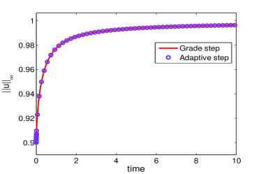
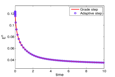
Figure 1: The solution in the maximum norm (left) and the discrete energy (right) vary against time until $T=10$ for Example 5.2 with the fractional order $\alpha=0.7$.

For a fixed fractional order $\alpha=0.7$, Figure 1 presents the solution in the maximum norm and the energy functional $E(t_{k})$ over the time interval $[0,T]$ with $T=10.$ The graded mesh with $\gamma=,3$ $N_{0}=30$ and $T_{0}=0.01$ in the starting interval $[0,T_{0}]$ is used to resolve the initial singularity. For $(T_{0},T]$ we first consider a uniform mesh with the total grid number $N_{1}=970$ (listed as Grade step). For comparison, we also consider an adaptive grids (listed as Adaptive step), and we use the adaptive time-stepping technique in the time interval $(T_{0},T]$ with the parameters $S_{a}=0.9$, $tol=10^{-3}$, and $\tau_{\min}=\tau_{N_{0}}=10^{-3}$ and $\tau_{\max}=10^{-1}$. It is learned in Figure 1 that the adaptive mesh provides good agreement with a fine uniform mesh. While the adaptive time-stepping strategy leads to a substantial decrease in the computational cost since the number of adaptive steps is 108, while the uniform mesh needs 970 steps.

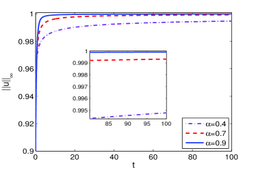
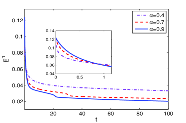
Figure 2: The maximum norm values (left) and the discrete energies (right) vary against time until $T=100$ for Example 5.2 with three fractional orders $\alpha=0.4,0.7$ and $0.9$.

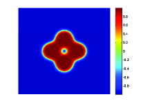
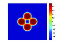
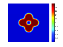
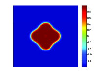
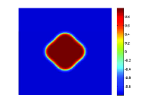
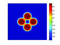
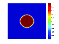
Figure 3: Solution snapshots of time-fractional Allen-Cahn equation at $t=1,10,50,100$ (from left to right) for fractional orders $\alpha=0.4$, $0.7$ and $0.9$ (from top to bottom).

Second, we investigate the equilibration process of the drops in Example 5.2 by using the adaptive strategy. Figure 2 compares the maximum norm values and the discrete energy functionals for three different fractional orders $\alpha=0.4,0.7$ and $0.9$ over a long-time interval $[0,100].$ We observe that the larger the fractional order $\alpha$, the faster the maximum norm value approaches 1, but the maximum norm values are always bounded by 1 for all cases. Similarly, the larger the fractional order $\alpha$, the faster the energy dissipates.

Figure 3 displays the snapshots of the solution contours for different fractional orders $\alpha=0.4,0.7$ and $0.9$. The same adaptive time-stepping technique is employed in the time interval $(T_{0},T]$ with the parameters $S_{a}=0.9$, $tol=10^{-3}$, $\tau_{\min}=\tau_{N_{0}}=10^{-3}$ and $\tau_{\max}=10^{-1}$. As time escapes, the four-drops merges into a single drop and shrinks progressively (due to the primitive problem dose not conserve the volume). Moreover, the larger the fractional order $\alpha$, the bigger the shrinkage.

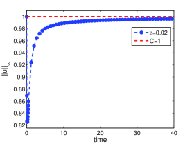
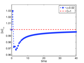
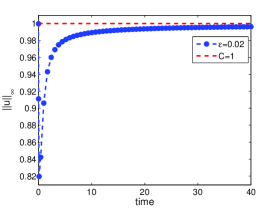
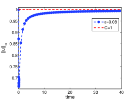
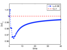
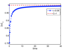
Figure 4: The solution in maximum norm for $\varepsilon=0.02$ (top) and $0.08$ (bottom) on different time meshes. Three meshes used in top figures: uniform mesh ($N=800$, $\tau=0.05$), uniform mesh ($N=60$, $\tau=0.67$) and graded mesh ($N=60$, $N_{0}=8$, $T_{0}=2$ and $\gamma=3$). Three meshes adopted in bottom figures: uniform mesh ($N=2000$, $\tau=0.02$), uniform mesh ($N=70$, $\tau=0.57$) and graded mesh ($N=70$, $N_{0}=4$, $T_{0}=1$ and $\gamma=3$).

Example 5.3

We next consider $\partial_{t}^{\alpha}u=\varepsilon^{2}\Delta u-f(u)$ on $\Omega=(0,1)^{2}\times(0,40]$ with the fractional order $\alpha=0.7$. The solution is computed with the spatial step $h=0.01$ using initial data $u_{0}=0.95\times{rand}(\mathbf{x})+0.05$, where $rand(\cdot)$ generates a random number in $(0,1)$.

We use this example to examine the discrete maximum principle by two different diffusive coefficients $\varepsilon=0.02,0.08$ and three different time-stepping approaches, see Figure 4. Notice that the graded meshes in the right figures put $N_{0}$ grid points with a proper grading parameter $\gamma$ inside the starting cell $[0,T_{0}]$, cf. Example 5.1, but use the uniform mesh with the time-step $\tau=(T-T_{0})/(N-N_{0})$ over the remainder interval $(T_{0},T]$. The try-and-error tests show that the maximum norm values are uniformly bounded by 1 provided the time-step size $\tau<0.67$ and $\tau<0.57$ for the two cases $\varepsilon=0.02$ and $\varepsilon=0.08$, respectively. As seen, the time-step constraint (3.9) is only sufficient to ensure the discrete maximum principle.

More interestingly, when the graded mesh is adopted near the initial time, the maximum norm values are still bounded by 1 even for larger time-steps ($\tau=0.73$ for $\varepsilon=0.02$ in the top right figure in Figure 4) in the remainder interval $(T_{0},T]$. This shows that a good resolution of initial singularity is also important to preserve the maximum principle.

6 Conclusions

We have proposed a second-order maximum principle preserving time-stepping scheme for the time-fractional Allen-Cahn equation under nonuniform time steps. Sharp maximum-norm error estimates the can reflect the temporal regularity are also presented. As our analysis is built on nonuniform time steps, we may resolve the intrinsic initial singularity by considering the graded meshes, and furthermore, we propose an adaptive time-stepping strategy for long-time simulations. Numerical experiments are presented to show the effectiveness of the proposed scheme.

We remark that the energy stability has not beed addressed in this work. Up to now we are unable to build up a discrete energy dissipation law for the second-order scheme (3.6)-(3.7). As seen in [28], the key issue is to prove the positive semi-definite of the quadratic form $\sum_{k=1}^{n}w_{k}\sum_{j=1}^{k}A_{k-j}^{(k)}w_{j}$. In fact, we can show the energy stability under uniform mesh using similar arguments as in [28]. However, on a general nonuniform mesh, it remains open to determine what kind of restrictions must be imposed on the discrete kernels $A_{n-k}^{(n)}$ so that $\sum_{k=1}^{n}w_{k}\sum_{j=1}^{k}A_{k-j}^{(k)}w_{j}$ is positive semi-definite. This will be part of our future studies.

References

- [1] A. Alikhanov. A new difference scheme for the time fractional diffusion equation. J. Comput. Phys., 280:424–438, 2015.
- [2] S.M. Allen and J.W. Cahn. A microscopic theory for antiphase boundary motion and its application to antiphase domain coarsening. Acta Metall, 27:1085–1095, 1979.
- [3] H Chen and M Stynes. Error analysis of a second-order method on fitted meshes for a time-fractional diffusion problem. J. Sci. Comput., 79(1):624–647, 2019.
- [4] M.H. Chen, P.C. Bollada, and P.K. Jimack. Dynamic load balancing for the parallel, adaptive, multigrid solution of implicit phase-field simulations. Int. J. Numer. Anal & Modeling, 16(2):297–318, 2019.
- [5] Q. Du, J. Yang, and Z. Zhou. Time-fractional Allen-Cahn equations: analysis and numerical methods. arxiv.1906.06584, 2019.
- [6] X. Feng and A. Prohl. Numerical analysis of the Allen-Cahn equation and approximation for mean curvature flows. Numer. Math., 94(1):33–65, 2003.
- [7] H. Gomez and T. J. Hughes. Provably unconditionally stable, second-order time-accurate, mixed variational methods for phase-field models. J. Comput. Phys., 230:5310–5327, 2011.
- [8] Zhen Guan, John S. Lowengrub, Cheng Wang, and Steven M. Wise. Second order convex splitting schemes for periodic nonlocal Cahn–Hilliard and Allen–Cahn equations. Journal of Computational Physics, 277:48–71, 2014.
- [9] R. Guo and Y. Xu. High order adaptive time-stepping strategy and local discontinuous galerkin method for the modified phase field crystal equation. Commun. Comput. Phys., 24(1):123–151, 2018.
- [10] T. Hou, T. Tang, and J. Yang. Numerical analysis of fully discretized Crank-Nicolson scheme for fractional-in-space Allen-Cahn equations. J. Sci. Comput., 72:1–18, 2017.
- [11] M. Inc, A. Yusuf, A. Aliyu, and D. Baleanu. Time-fractional Cahn-Allen and time-fractional Klein-Gordon equations: Lie symmetry analysis, explicit solutions and convergence analysis. Physica A Stat. Mech. Appl., 493:94–106, 2018.
- [12] S. Jiang, J. Zhang, Z. Qian, and Z. Zhang. Fast evaluation of the Caputo fractional derivative and its applications to fractional diffusion equations. Comm. Comput. Phys., 21:650–678, 2017.
- [13] B. Jin, R. Lazarov, and Z. Zhou. An analysis of the L1 scheme for the subdiffusion equation with nonsmooth data. IMA J. Numer. Anal., 36:197–221, 2016.
- [14] Y. Li, Y. Choi, and J. Kim. Computationally efficient adaptive time step method for the Cahn-Hilliard equation. Comput. Math. Appl., 73:1855–1864, 2017.
- [15] Z. Li, H. Wang, and D. Yang. A space-time fractional phase-field model with tunable sharpness and decay behavior and its efficient numerical simulation. J. Comput. Phys., 347:20–38, 2017.
- [16] H.-L. Liao, D. Li, and J. Zhang. Sharp error estimate of nonuniform L1 formula for time-fractional reaction-subdiffusion equations. SIAM J. Numer. Anal., 56:1112–1133, 2018.
- [17] H.-L. Liao, W. Mclean, and J.Zhang. A second-order scheme with nonuniform time steps for a linear reaction-sudiffusion problem. arXiv:1803.09873v4, 2018. in review.
- [18] H.-L. Liao, W. Mclean, and J. Zhang. A discrete Grönwall inequality with application to numerical schemes for subdiffusion problems. SIAM J. Numer. Anal., 57:218–237, 2019.
- [19] H.-L. Liao, Y. Yan, and J. Zhang. Unconditional convergence of a fast two-level linearized algorithm for semilinear subdiffusion equations. J. Sci. Comput., 80(1):1–25, 2019.
- [20] H.-L. Liao, Y. Zhao, and X. Teng. A weighted ADI scheme for subdiffusion equations. J. Sci. Comput., 69:1144–1164, 2016.
- [21] Y. Lin and C. Xu. Finite difference/spectral approximations for the time-fractional diffusion equation. J. Comput. Phys., 225(2):1533–1552, 2007.
- [22] H. Liu, A. Cheng, H. Wang, and J. Zhao. Time-fractional Allen-Cahn and Cahn-Hilliard phase-field models and their numerical investigation. Comp. Math. Appl., 76:1876–1892, 2018.
- [23] W. McLean and K. Mustapha. A second-order accurate numerical method for a fractional wave equation. Numer. Math., 105:481–510, 2007.
- [24] Z. Qiao, Z. Zhang, and T. Tang. An adaptive time-stepping strategy for the molecular beam epitaxy models. SIAM J. Sci. Comput., 33:1395–1414, 2011.
- [25] J. Shen and X. Yang. Numerical approximations of Allen-Cahn and Cahn-Hilliard equations. Discret. Contin. Dyn. Syst., 28:1669–1691, 2010.
- [26] M. Stynes, E. OŔiordan, and J. Gracia. Error analysis of a finite difference method on graded meshes for a time-fractional diffusion equation. SIAM J. Numer. Anal., 55(2):1057–1079, 2017.
- [27] Z. Sun and X. Wu. A fully discrete difference scheme for a diffusion-wave system. Appl. Numer. Math., 56(2):193–209, 2006.
- [28] T. Tang, H. Yu, and T. Zhou. On energy dissipation theory and numerical stability for time-fractional phase field equations. arXiv:1808.01471v1, to appear in SIAM J. Sci. Comput., 2019.
- [29] C. Xu and T. Tang. Stability analysis of large time-stepping methods for epitaxial growth models. SIAM J. Numer. Anal., 44:1759–1779, 2006.
- [30] Z. Zhang and Z. Qiao. An adaptive time-stepping strategy for the Cahn-Hilliard equation. Comm. Comput. Phys., 11:1261–1278, 2012.